High-Order Fully General-Relativistic Hydrodynamics: new Approaches and Tests
Abstract
We present a new approach for achieving high-order convergence in fully general-relativistic hydrodynamic simulations. The approach is implemented in WhiskyTHC, a new code that makes use of state-of-the-art numerical schemes and was key in achieving, for the first time, higher than second-order convergence in the calculation of the gravitational radiation from inspiraling binary neutron stars [1]. Here, we give a detailed description of the algorithms employed and present results obtained for a series of classical tests involving isolated neutron stars. In addition, using the gravitational-wave emission from the late inspiral and merger of binary neutron stars, we make a detailed comparison between the results obtained with the new code and those obtained when using standard second-order schemes commonly employed for matter simulations in numerical relativity. We find that even at moderate resolutions and for binaries with large compactness, the phase accuracy is improved by a factor or more.
pacs:
04.25.Dm, 04.30.Db, 95.30.Lz, 95.30.Sf1 Introduction
The accurate modeling of gravitational waves from the late-inspiral and merger of binary neutron stars can only be achieved within the framework of numerical relativity and exploiting the tools of computational relativistic hydrodynamics. Assuming the simplest physical scenarios, i.e. irrotational binaries in quasi-circular orbits, and idealized equations of state, i.e. polytropic of Gamma-law, very accurate numerical-relativity waveforms for binary neutron stars are nowadays available, e.g. [2, 3, 4, 5, 1]. However, obtaining good-quality waveforms to fully cover the large parameter space of possible binary-neutron-star configurations, equations of state and compactnesses, seems to be out of the reach for current-generation codes. The main reason behind this difficulty is to be found in the small convergence order, i.e. , typical of general-relativistic hydrodynamics codes, and which has a number of undesired consequences. Among these, the fact that obtaining high-accuracy waveforms from low-order codes requires very high spatial resolutions (and hence very high computational costs), or the fact that the analysis of the waveforms is spoiled by the large phase uncertainties typical of these simulations. Both of these difficulties can be resolved in part by employing new, state-of-the-art schemes that are able to go over the second-order of convergence typical of general-relativistic hydrodynamics codes. Using these techniques, we were recently able to achieve, for the first time, higher than second-order convergence in both the phase and amplitude of the gravitational-wave radiation from binary neutron stars [1]. These new advances could potentially enable a more systematic study of the gravitational radiation from binary neutron stars, similarly to what has been done for the case of binary black-holes, e.g. [6, 7].
The goal of this paper is to give a full description of the methods we employed in [1] and to describe in detail our new high-order, high-resolution shock-capturing, finite-differencing code: WhiskyTHC, which represents the extension to general relativity of the THC code presented in [8]. When compared with other high-order relativistic hydrodynamics codes, such as wham [9] and ECHO [10, 11], this is the first higher-than-second-order code that works in full general relativity, i.e. with dynamical spacetime, and in three spatial dimensions.
First, we demonstrate the capabilities of the new code in a series of tests involving the evolution of isolated neutron stars. More specifically, we show that the code is able to yield long-term and accurate evolutions of stable and unstable stars. We measure the accuracy of the code for the case of an unstable star collapsing to a black hole and show that we are able to achieve third-order convergence.
Second, we consider the performance of the code in calculating the inspiral and merger of binary neutron stars in quasi-circular orbits. We show higher than second-order convergence for the phase and the amplitude of the gravitational waves produced in this process. When compared with the performance of our previous Whisky code, which adopts the standard second-order schemes commonly employed for matter simulations in numerical relativity, we can show that the new code is able to yield a decrease in the phase error of a factor for simulations with the same resolution and with similar computational costs.
The rest of this paper is organized as follows. In Section 2 we quickly recall the equations of general-relativistic hydrodynamics and the CCZ4 formalism used to evolve the spacetime for the tests presented here. In Section 3 we give a quick summary of the numerical methods that we employed, as well as a detailed description of the treatment of the fluid–vacuum interfaces, which was one of the main challenges in the application of higher-order numerical schemes to binary-neutron-stars simulations. In Section 4 we present the results obtained with our code in a series of representative tests involving the evolution of isolated neutron stars, with particular focus on the properties of the different vacuum treatments implemented in the code. In Section 5 we present results obtained in the case of binary neutron stars and, finally, we dedicate Section 6 to the discussion of our results and to the conclusions.
We use a spacetime signature , with Greek indices running from 0 to 3 and Latin indices from 1 to 3. We also employ the standard convention for the summation over repeated indices. Unless otherwise stated, all quantities are expressed in a system of units in which .
2 General-Relativistic Hydrodynamics
In this work we adopt the usual 3+1 formalism, e.g. [12], to decompose spacetime into space-like hypersurfaces with normal , where is the lapse function and is the shift vector. Within this formalism the spacetime metric is split as
where is the spatial three-metric metric, which, together with the extrinsic curvature , being the Lie derivative along , fully determines the geometry of each leaf of the foliation. Furthermore we will indicate with and the Ricci tensor and scalar associated with the Levi-Civita connection on the spacelike hypersurfaces of the foliation, respectively.
The matter content of the spacetime is described through its energy-momentum tensor , which, within the 3+1 split of spacetime, can be decomposed in its time, spatial and mixed components as (see, e.g. , [13])
| (1) |
Finally, we will use the convention of raising and lowering indices of spatial tensors with the (spatial) three-metric, unless otherwise stated.
2.1 Spacetime Evolution Equations
For the solution of the Einstein equations we adopt the covariant and conformal formulation of the Z4 equations (CCZ4). We recall that the Z4 formulation can be obtained from the covariant Lagrangian
| (2) |
by means of a Palatini-type variational principle [14], where is the metric determinant. The variational principle yields the field equations
| (3) |
as well as a set of constraints fixing the connection
| (4) |
and the algebraic constraint
| (5) |
If Eq. (5) is satisfied then Eqs. (3) and (4) reduce to the standard Einstein field equations. Otherwise gives a measure of the deviation of the solution from the one of the original Einstein equations. In addition we point out that it is possible to show that the condition that the first derivatives of vanish amounts to imposing the ADM momentum and Hamiltonian constraints [15].
The key idea of the Z4 formalism is to develop a set of evolution equations starting from the Lagrangian (2), without explicitly enforcing (5), i.e. treating as a new independent variable. The resulting set of equations is then strongly hyperbolic, i.e. free from the zero-speed modes of the original ADM system, and the solution of the Einstein equations is obtained exploiting the fact that the Z4 evolution system preserves the constraint (5), i.e. . In particular, if the initial-data is constraint satisfying, the Z4 evolution recovers the solution of the Einstein equations, even though is an evolved variable. In practice, however, small numerical errors introduce constraint violation during the evolution, for this reason the Z4 system is usually modified, with the addition of terms that cancel out in the case in which the constraints are satisfied, to ensure that eventual constraint violations are propagated away and damped exponentially [16].
The version of Z4 that we employ was recently introduced by [17] and is based on a conformal decomposition of the original Z4 system and aims at exploiting well-tested gauge conditions together with the constraint propagation and damping properties of the original Z4 formulation. The CCZ4 system then reads [17]
| (6a) | |||
| (6b) | |||
| (6c) | |||
| (6d) | |||
| (6e) | |||
| (6f) | |||
where , , is the conformal metric with unit determinant , while the extrinsic curvature is split into its trace and its trace-free components
| (6g) |
The three-dimensional Ricci tensor is split into a part containing conformal terms and another one containing space derivatives of the conformal metric , defined as
| (6h) | |||
| (6i) |
We adopt the constrained approach from [17] in order to enforce the constraints of the conformal formulation; in other words we enforce the condition and .
The evolution variable of the original Z4 formulation is now included in the variable of the CCZ4 formulation
| (6j) |
where
| (6k) |
Finally, and are constants associated with the constraint damping terms and is an extra constant used to select among different variants of the formulation. In this paper we take and and recall that the CCZ4 formulation is publicly available through the Einstein Toolkit [18, 19].
2.2 Relativistic Hydrodynamics
Since we assume the neutron-star matter to be described as a perfect fluid, the corresponding energy-momentum tensor is given by [13]
| (6o) |
where is the rest-mass density, is the fluid four-velocity, is the pressure and is the specific enthalpy. The equations of motion for the fluid are the “conservation” of the stress-energy tensor
| (6p) |
and the baryon number conservation
| (6q) |
These two set of equations are closed by an equation of state (EOS) , and we here assume a simple ideal-fluid (or Gamma-law EOS)
| (6r) |
with case. In some of the tests we also consider the restriction of this EOS to the isentropic case, i.e. the polytropic EOS:
| (6s) |
Although here we use idealized EOSs, the code can make use of the generic EOS infrastructure developed in the Whisky code and recently presented in [22], which has full support for thermal and composition-dependent tabulated EOSs.
Equations (6p) and (6q) are solved in conservation form following the approach by first proposed by [23], i.e. the Valencia formulation, and written as
| (6t) |
with a vector of primitive variables
| (6u) |
and conservative variables
| (6v) |
The fluxes are
| (6w) |
while the sources functions are given by
In the expressions above the fluid three-velocity measured by the normal observer is defined as
| (6x) |
while the advection velocity relative to the coordinates is
| (6y) |
and the Lorentz factor is defined as . Finally, we denoted with the determinant of the spatial metric and we have used the fact that .
3 THC: A Templated Hydrodynamics Code
In this Section we give an overview of WhiskyTHC. First, we describe the numerical methods used and then a detailed description of our treatment of fluid–vacuum interfaces, which is one of the key problems to be addressed in order to attain stable binary evolution, especially with high-order codes.
WhiskyTHC results from the merger of two codes: Whisky [24] and THC [8]. It inherited from THC the use of high-order flux-vector splitting finite-differencing techniques and from Whisky the new module for the recovery of the primitive quantities as well as the new equation of state framework recently introduced in [22]. This code can make use of tabulated, temperature and composition dependent equation of states, but here we are concerned only with Gamma-law and polytropic evolutions. More specifically WhiskyTHC solves the equations of general-relativistic hydrodynamics in conservation form (6t) using a finite-difference scheme. It employs flux reconstruction in local-characteristic variables using the MP5 scheme, for which it uses the explicit expression for the eigenvalues and left and right eigenvectors which can be found in, e.g. [13].
The spacetime is evolved using a standard finite-difference method where all the derivatives, with the exception of the terms associated with the advection along the shift vector, for which we use a stencil upwinded by one grid point, are computed with a centered stencil. Typically all these terms are computed with a fourth-order accurate scheme, but sixth and eighth order are also available. To ensure the nonlinear stability of the scheme we add a fifth-order Kreiss-Oliger style artificial dissipation [25]; more details on the code can be found in [26].
Finally, the time evolution and the coupling between the hydrodynamic and the spacetime solvers is done using the method of lines (MOL), either with the optimal, strongly-stability preserving third-order Runge-Kutta scheme, or with the standard fourth-order one.
3.1 Numerical Methods
For simplicity we consider, at first, the case of a uniform grid
| (6z) |
The equations of relativistic hydrodynamics (6t) are written on such a grid using the method of lines in a semidiscrete, dimensionally unsplit way as
| (6aa) |
where is the value of a generic quantity, , at , while is a high-order, non-oscillatory, approximation of at , whose explicit expression still needs to be specified.
To illustrate how we compute the discrete derivatives on the right-hand-side of (3.1) it is useful to make a step back and consider, first a simpler scalar hyperbolic equation in one dimension, i.e.
| (6ab) |
We introduce a uniform grid, , and define, for any function, the volume averages
| (6ac) |
A reconstruction operator, , is a nonlinear operator yielding a high-order approximation of at a given point using its volume averages, . Since can be discontinuous, we distinguish two different reconstruction operators, and , called the left-biased and right-biased reconstruction operators, such that
| (6ad) | |||
| (6ae) |
where we have used the notation to remark that is an operator that acts on a set of averages , and where is the order of the reconstruction operator . Hereafter we will use the notation and to denote the reconstructed values in using and respectively, i.e. .
| (6af) | |||
| (6ag) |
Our code implements a wide range of reconstruction operators, from the second-order minmod to the seventh-order weighted essentially non-oscillatory (WENO) reconstructions, but all the calculations in this paper were performed using the fifth-order monotonicity preserving (MP5) scheme, which, as discussed in [8], represent a good compromise between robustness and accuracy.
The reconstruction operators are the core components of both finite-volume and finite-difference schemes. In a finite-volume scheme they are used to compute the left and right state to be used in the (usually approximate) Riemann solver to compute the fluxes (see, e.g. [13] for details). In a finite-difference scheme, instead, they are used to compute the above mentioned non-oscillatory approximation of . Following [27] we introduce a function and such that
| (6ah) |
that is, the average of between and corresponds to the value of at . Next, we note that
| (6ai) |
where both (6ah) and (6ai) are exact expressions. Hence, by using the usual reconstruction operators of order to reconstruct , one obtains a corresponding accurate approximation of order of the derivative at . Note that is never actually computed at any time during the calculation as we only need the values of at the grid points, i.e. .
In order to ensure the stability of the resulting scheme, one has to take care to upwind the reconstruction appropriately. Let us first consider the case in which . If we set
| (6aj) |
and
| (6ak) |
then
| (6al) |
gives the wanted high-order approximation of at .
In the more general case, where the sign of needs to be determined, in order to compute , we have to split in a right-going flux, , and a left-going one, , i.e. , and use the appropriate upwind-biased reconstruction operators separately on both parts, in order to guarantee the stability of the method.
There are several different ways to perform such a split and in our code we implemented two of them: the Roe flux-split, i.e.
| (6am) |
where , and the Lax-Friedrichs or Rusanov flux-split [28], i.e.
| (6an) |
where the maximum is taken over the stencil of the reconstruction operator. The Roe flux-split is less dissipative and yields a computationally less-expensive scheme, since only one reconstruction is required instead of two, but its use can result in the creation of entropy-violating shocks in the presence of transonic rarefaction waves (see, e.g. [29]), and it is also susceptible to the carbuncle (or odd-even decoupling) phenomenon [30]. To avoid these drawbacks, we switch from the Roe to the Lax-Friedrichs flux split when or are not monotonic within the reconstruction stencil.
We now go back to the more general system of equations (6t). The derivatives can be computed following the procedure outlined above on a component-by-component basis. This approach is commonly adopted in the case of low-order schemes, but it often results in spurious numerical oscillations in the high-order (usually higher then second) case. To avoid this issue the reconstruction should be performed on the local characteristic variables of the systems. To avoid an excessively complex notation, let us concentrate on the fluxes in the -direction; in this case, to reconstruct , we introduce the Jacobian matrices
| (6ao) |
where is an average state at the point where the reconstruction is to be performed. In our code and are computed as a simple average of the left and right states [8], while, in order to avoid creating unphysical values in the velocity, is computed from the averages of in the left and right states.
Hyperbolicity of (6t) implies that is invertible and the generalised eigenvalue problem
| (6ap) |
has only real eigenvalues, , and independent, real right-eigenvectors, [31] (see, e.g. [32, 13] for the explicit expressions of the eigenvalues and eigenvectors). We will denote with the matrix of right eigenvectors, i.e.
| (6aq) |
and with its inverse. We define the local characteristic variables
| (6ar) |
and compute doing a component-wise reconstruction, where is used in place of and in place of in Eq. (6an). Finally, we set
| (6as) |
This procedure is repeated in the other directions and yields the wanted approximations of the terms in . In all of the results presented here the reconstruction is typically performed in local characteristic variables. Exceptions are low-density points (at least for some of the atmosphere prescriptions; more on this below) or points which, on the basis of the value of the lapse function, we estimate being inside an apparent horizon. In these cases we switch to the component-wise reconstruction of the fluxes with Lax-Friedrichs flux-split.
The primitive variables are recovered after each sub-step using a numerical root-finding procedure. In particular WhiskyTHC uses the EOS and primitive variables recovery framework recently developed for the Whisky code and described in details in [22]. The only differences between our approach and the one discussed there is that 1) we do not alter the conservative quantities to match the primitive ones in the case in which adjustments have been made, 2) to ensure the well behaviour of the eigenvectors (which become degenerate if the sound speed goes to zero) we enforce a floor on (more on this in the next Section). The reason why we do not alter the conserved quantities in case of failures is that we prefer to rely on the evolution to bring them back into the physically allowed region, instead of changing them in an arbitrary manner. We also note that any adjustment made in the recovery can be simply interpreted as an error in the calculation of the flux/source terms
Finally, our code has been tested using a rather basic subset of the features supported by Carpet [33], the AMR driver of the Cactus computational toolkit [34] on top of which our code is built. Carpet supports Berger-Oliger-style mesh refinement [35, 36, 37] with sub-cycling in time and refluxing. At the moment, our code has been tested only with static grid refinement. It supports sub-cycling in time, but not refluxing. While we have plans to implement refluxing and test high-order prolongation operators in order to use dynamical grids, we also note that these features are not of fundamental importance for the study of gravitational waves from inspiraling binary neutron stars, which is the main aim of our code.
3.2 Treatment of Vacuum Regions
The treatment of interfaces between vacuum region and fluid regions is one of the most challenging problems in Eulerian (relativistic) hydrodynamics codes (see e.g. [38, 39, 40]), especially when studying near-equilibrium configuration, such as an oscillating compact star, having large density gradients close to the surface and over long timescales. The most commonly used approach to treat vacuum regions is to fill them with a low-density fluid, the “atmosphere”, such that if a fluid element is evolved to have a rest-mass density below a certain threshold, it is set to have a floor value and zero coordinate velocity [41, 24]. This approach works reasonably well for standard second-order codes and has been adopted by the vast majority of the relativistic-hydrodynamics codes, but it is problematic for higher-order codes [42]. The reason is that small numerical oscillations can easily result in the creation of very low-density regions that with the prescription for the floor, violating the conservative character of the equations and creating artificially mass, energy and momentum. As a result, they are subsequently amplified, ultimately destabilizing the evolution. The situation is even more complicated for a code, such as ours, which relies on characteristic variables as they become degenerate in the low-density, low-temperature limits.
We notice that for many applications, such as the inspiral of binary neutron stars (at least up to contact), or the oscillation of single stars, the treatment of the stellar surface is one of the main challenges and the only reason why low-order, but robust shock capturing codes are commonly used. Indeed the problem of the vacuum treatment is one of the main obstacles on the road to high-order general-relativistic hydrodynamics codes. For this reason, it is instructive to address this problem in detail as we do in the following.
However, before going into the details of the treatment, it is useful to make two rather general remarks. First, we should point out that the MP5 scheme is remarkably robust even in conjunction with the most basic atmosphere treatment that we implemented, i.e. one in which no additional modification is made on the scheme at the interface between vacuum and fluid region, beside the imposition of a minimum rest-mass density level (more on this below). In our preliminary tests, other schemes, such as WENO5, which do not enforce the monotonicity of the reconstruction, could not yield stable evolutions even for single stars in the Cowling approximation. Second, most of the problems with the atmosphere appear in points where the surface of the star is aligned with the grid, because along these directions the numerical dissipation is minimal. These artefacts, that we discuss in more detail in the next Section, are easily “fixed” with the use of extra numerical dissipation close to the surface of the star. Keeping this in mind, we now give the details of the three different prescriptions that we developed for the treatment of the low-density regions.
3.2.1 Standard Atmosphere Treatment
The first prescription is what we call the “ordinary MP5” approach. It follows the lines of what is most commonly done to treat vacuum in general-relativistic hydrodynamics. First, we choose a minimum rest-mass density , which we take to be, typically, in the range , being some reference rest-mass density (normally the initial maximum rest-mass density). Second, we choose a tolerance parameter, , typically , chosen to avoid excessive oscillations of the fluid–vacuum interface so that points where the rest-mass density falls below , are set to atmosphere. In particular, the rest-mass density is set to , the velocity to zero and the internal energy is calculated assuming a polytropic EOS. In addition, we enforce a floor for the conserved energy density , .
As we show below, this approach, is already perfectly adequate for inspiraling binary neutron stars, but it might have problems in the case of slowly moving vacuum-fluid interfaces aligned with the grid, especially in the case of isentropic evolutions where the surface remains a sharp interface and no spurious heating can occur.
3.2.2 Improved Atmosphere Treatment
In order to improve our atmosphere treatment, we introduced an alternative method in which we increase the level of dissipation of the scheme by switching to the component-wise Lax-Friedrichs flux split below a certain rest-mass density. Typical values for this new threshold are chosen so that the first one or two grid points in the stellar interior are evolved using the Lax-Friedrichs flux split. The use of component-wise reconstruction, as opposed to characteristic-wise, is done to avoid problems due to the degeneracy of the characteristic variables close to vacuum and to avoid polluting quantities, such as the linear momentum, with the numerical errors present in the internal energy (which is typically large in the immediate vicinity of the atmosphere). This is what we refer to as “MP5+LF” approach.
This latter approach is more robust, but can also result in the creation of artefacts in the case in which low-density matter is ejected from the stellar surface. In this case, the fluid typically presents a rather smooth interface with vacuum, so that one would expect to be able to treat it with high accuracy. Unfortunately, as we show in the next Section, if the rest-mass density of the ejecta falls below the Lax-Friedrichs threshold, the use of a component-wise reconstruction yields a rather oscillatory solution, with the creation of patchy regions of lower/higher rest-mass density in very dynamical situations (cf. second panel in Figure 7 and the discussion there).
3.2.3 Positivity Preserving Limiter
Overall neither of the previous methods is completely satisfactory. For this reason we propose here a novel approach based on the use of the positivity preserving limiter recently proposed by [43], which is significantly simpler to implement than the “classical” positivity-preserving limiters already proposed in the literature, e.g. [44, 45, 46, 47].
For the sake of completeness, we give here a brief overview of the key ideas presented in [43], to which we refer to for a more complete presentation. To keep the notation simple we consider, at first, a scalar conservation law in one dimension
| (6at) |
We notice that any scheme able to guarantee the positivity of over one first-order Euler timestep, will automatically guarantee positivity when used with any SSP time integrator, as in these schemes the time update is always constructed as a convex combination111We recall that a convex combination of a set of vectors, , is a combination of the form , where and . of Euler steps. For this reason we consider a discretization of (6at) of the form
| (6au) |
If we let , then the previous can be written as
| (6av) |
where and . Clearly, if and are positive, so will be . The key observation made in [43] is that, if and are computed with the first-order Lax-Friedrichs scheme with , being the largest propagation speed, then [44].
The idea is to modify Eq. (6au) as
| (6aw) |
where is the high-order flux of the original scheme, is the flux associated with the first-order Lax-Friedrichs scheme, and is chosen to be the maximum value such that both and are positive. In regions where the solution is far from vacuum, , so that the high-order fluxes are used (and in particular the formal order of accuracy of the scheme remains unchanged). In regions close to vacuum, it is always possible to find some such that positivity is guaranteed, since for the scheme reduces to the Lax-Friedrichs scheme, which is known to be positivity preserving.
The multi-dimensional extension of Eq. (6av) is done in a component-by-component fashion. For instance in three dimensions (6av) becomes
| (6ax) | |||||
where are positive constants such that , typically chosen so as to be equal to (but see the remarks at the end of the Section). The limiter at each interface is then chosen enforcing positivity of the terms in the round brackets.
This approach can then be easily extended to systems of equations [43]. In particular, [43] constructed a limiter able to guarantee the positivity of rest-mass density and pressure for the classical equations of hydrodynamics also in the case in which source terms are present222Note that in this case a smaller timestep might be required, depending on the nature of the source terms.
In the general-relativistic case, it is not trivial to enforce the positivity of the pressure, especially for tabulated EOS, because of the presence of complex source terms in the energy equations. For this reason, as was the case for the atmosphere treatment, we need to enforce positivity of the pressure with the imposition of a floor on . On the other hand, the continuity equation
| (6ay) |
where and , is formally equivalent to the Newtonian continuity equation after the identification
| (6az) |
thus one can construct a scheme ensuring the positivity of by simply adopting the prescriptions used by [43] to guarantee the positivity of the density for the Newtonian Euler equations.
Some comments should be made on the positivity preserving limiter. First, the positivity preserving limiter is not directly a way to treat vacuum–fluid interfaces in a physically accurate way, for the simple reason that the fluid model is not adequate to represent such transitions. A proper modeling of the stellar surface can only be done by treating it as a free boundary of the problem determined by the balance between inertial and gravitational forces on the fluid as done, for instance, in [39]. For this reason its use does not free us from having a low-density fluid everywhere or from having to manually enforce that . This may be necessary because in some situations, for instance at the surface of a star, the high-order fluxes and the Lax-Friedrichs fluxes can differ by several orders of magnitude, so that small floating-point errors can drift the conserved density, , below the minimum. This is done by simply resetting to whether , without changing the other quantities.
What the positivity preserving limiter does, however, is to ensure local conservation of the solution up to floating-point precision. This is because the floor for the fluid’s rest-mass density can be arbitrarily small and does not require any tuning. As a result, de-facto it prevents the scheme from extracting/losing mass from/to the atmosphere because of numerical oscillations. In contrast, the classical atmosphere prescriptions usually work only in a limited range of and as these coefficients must be tuned in order to achieve a balance between the amount of mass extracted from the atmosphere (which typically increases as decreases) and the mass lost into it (which typically increases as increases). With the positivity preserving limiter instead, in situations where we need to reset , we are guaranteed that this correction is of the order of the floating-point precision with respect to the typical rest-mass densities we are actually interested in tracking.
The way in which we use the positivity preserving limiter is rather simple: we fill the vacuum with a low rest-mass density floor at the beginning of a simulations and we let it evolve freely, only relying on the positivity preserving limiters to ensure its proper behaviour. This typically results in the creation of accretion flows onto our compact objects. However, given the low rest-mass density of the floor, which we take to be (i.e. below floating-point precision!), the effects of this artificial accretion are completely negligible.
To avoid problems with the decomposition of the Jacobian in eigenvalues and eigenvectors, we also switch to component-wise reconstruction below a certain rest-mass density, typically , but this, in contrast to the prescription outlined in the previous Section, has little dynamical effect as flows at those densities are, anyway, completely dominated by numerical effects. Moreover, as we show in the next Section, even if the floor rest-mass density is taken to be unnecessarily large, the use of positivity preserving limiters results in much smaller perturbations with respect to the use of a more traditional atmosphere treatment.
Finally, a comment concerning the timestep constraint, as this may be seen as the only real limitation of the positivity preserving approach. For the scheme to ensure positivity in the multi-dimensional case, one must ensure . Since and , being the number of dimensions, this results in a rather stringent Courant-Friedrichs-Lewy (CFL) condition. In practice we find our scheme to be robust even for much larger timesteps, probably because the advection velocity in the low rest-mass density regions is typically smaller than the maximum velocity and because Lax-Friedrichs scheme is actually positivity preserving even with Courant factor in one dimension [46] [ in dimensions, even though it is not possible to guarantee that and in Eq. (6av) are separately positive]. In order to use larger timesteps, we simply compute the value of the limiter assuming , as in the one-dimensional case (note this does not mean that we evolve using (6ax) with the ’s equal to one), and we set it to zero (i.e. we use Lax-Friedrichs fluxes) when it is not possible to enforce the positivity of and . We have found this procedure to be sufficient to prevent negative densities from occurring (at least at to a reasonable extent) and to be computationally much less expensive with respect to the approach in which .
4 Isolated Neutron Stars
In this Section we describe a series of representative tests that we performed with WhiskyTHC in the case of single, isolated, nonrotating neutron stars (or TOVs from Tolman-Oppenheimer-Volkoff [48, 49]). First, we present the results obtained in the Cowling approximation, i.e. without evolving the spacetime, for perturbed, oscillating stars. Then we proceed to analyze the case of linear oscillations of stable stars in full general relativity (GR). Finally, we show the results obtained for the evolution of unstable stars: both for the migration and for the collapse to a black hole. The focus of our discussion is mostly on the effects of the different prescriptions for the treatment of the atmosphere. Hereafter we will denote the basic treatment as “MP5”, the enhanced treatment with extra dissipation on the surface as “MP5+LF”, and the positivity preserving treatments as “MP5+PP”.
4.1 Linear Oscillations: Cowling Approximation
The first test that we consider is the long-term evolution of a perturbed, isolated, nonrotating, neutron star in the Cowling approximation. The goal of this test is to assess the impact on the accuracy of the three different atmosphere treatments over long timescales. We consider a model described by the polytropic EOS with and . The initial central rest-mass density is , yielding a model with an ADM mass of . The initial velocity is perturbed with the injection of a radial eigenfunction that is exact in the Cowling approximation. The maximum amplitude of the perturbation is and the initial perturbation is ingoing.
We evolve this model for , i.e. dynamical timescales, using our different prescriptions for the atmosphere. Our fiducial resolution is so that the radius of the star is covered with grid points. In order to make a fair comparison, we use the same atmosphere threshold for all the methods, , and evolve all the models with the third-order SSP-RK3 with . The gravitational source terms are computed using sixth-order finite differencing. Finally, the evolution is computed only in the octant and we assumed reflection symmetry across the and planes.
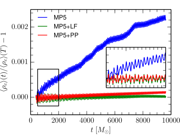
The evolution of the central rest-mass density, , is shown in Figure 1. In particular, in order to highlight the secular trend of the data, we show a moving average of defined as
| (6ba) |
where , being the frequency of the -mode from linear perturbation theory. All the different prescriptions yield very similar evolutions of the central rest-mass density which presents a series of slowly damped oscillations. The pulsation frequency agrees, to within the nominal error of the discrete Fourier transform, with the one expected from linear perturbation theory in the Cowling approximation. The power-spectrum also shows small contributions from higher-order overtones (i.e. more than a factor ten smaller than the -mode) as well as an even smaller nonlinear component at integer multiples of the -mode frequency. In the case of the MP5+LF prescription, we verified that the nonlinear component decreases with decreasing perturbation amplitudes and that it is not distinguishable from the background noise for perturbation amplitudes . The ordinary MP5 prescription also shows a small secular increase in the central rest-mass density. Apart from this, all the schemes appear to be able to yield very clean oscillations.
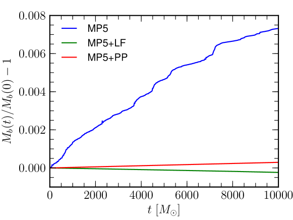
The difference between the different schemes can be better appreciated by looking at Figure 2 where we show the evolution of the total rest mass
| (6bb) |
for the different models. Overall, the rest-mass conservation is at acceptable levels for all the methods, i.e. , but the ordinary MP5 prescription is clearly the one with the largest error, as it shows larger variations with respect to the other schemes. This, in turn, is responsible for the secular drift mentioned earlier (an increase in the total rest mass leads to an increase in the central rest-mass density). The Lax-Friedrichs flux-switch at the surface, instead, results in a steady loss of matter which is slowly diffused into the atmosphere, while the MP5+PP approach yields a steady increase in the rest mass because of the accretion of the low-density floor which is continuously “injected” from the outer boundary (we simply fix the rest-mass density in the ghost regions at the outer boundary to its initial value).
MP5

MP5+LF
MP5+PP
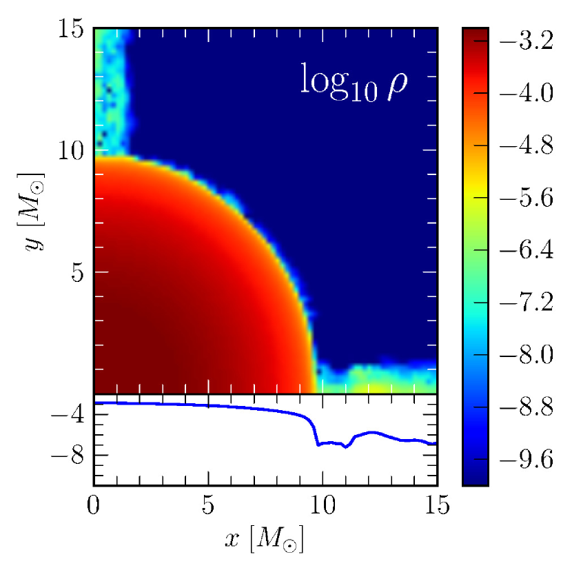
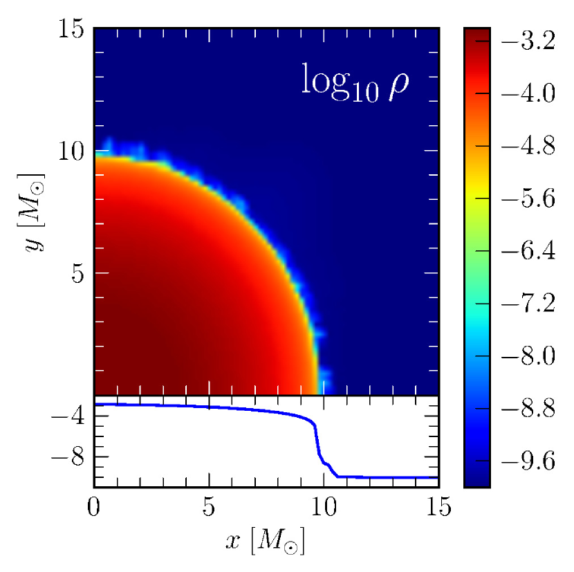
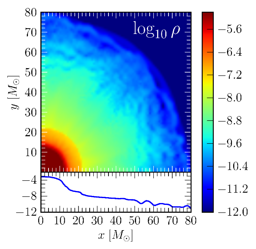
The reason for the bad behaviour of the standard MP5 prescription is that, as anticipated in the previous Section, it lacks a sufficient amount of numerical dissipation in the case of surfaces aligned with the grid and especially for polytropic evolutions, such as the ones we show here. This is clearly seen in Figure 3 where we show a two-dimensional cut of the rest-mass density, in scale, at a representative time during the evolution. One can clearly see the appearance of “jets” of low-density matter () aligned with the coordinate directions (see bottom part of each panel for a one-dimensional cut along the -direction). These “jets” are launched at seemingly random times from the surface of the star, when the numerical errors “extract” from the atmosphere a large enough amount of rest mass. What happens is that the numerical oscillations create an imbalance at the surface of the star: the excess density coming from the atmosphere generates a pressure which is only balanced by the “potential barrier” at the surface of the star given by the double threshold on the rest-mass density floor. As soon as the pressure is large enough, part of the matter is ejected in one of these streams. This process effectively results in the increase of the total rest mass of the star because only part of this extra matter is actually lost from the outer boundary. In contrast, we can see that, with the addition of extra numerical dissipation at the surface of the star, these artefacts are completely suppressed, as shown for the MP5+LF case. This happens partly because dissipation prevents the scheme from extracting too much matter out of the atmosphere and partly because it diffuses the numerical errors back into the floor. Finally, the positivity-preserving evolution does not show any kind of numerical ejecta out of the star’s surface because of its conservative nature. On the other hand it is affected by the accumulation of matter at the fluid-vacuum interface. As commented before, this accumulation can be greatly reduced by lowering the floor rest-mass density and it is also somewhat less severe for the Gamma-law EOS case, where the floor accretion is regulated by the thermal pressure.
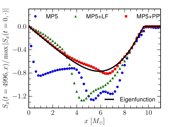
The differences between the various methods are even more evident if we look at sensitive quantities such as the linear momentum in the radial direction. At the initial time it has a profile given by the eigenfunction of the -mode in the Cowling approximation. In the linear regime one would expect the linear momentum to simply oscillate with the -mode frequency. On the other hand, in a simulation, because of numerical errors, the profile of the eigenfunction is gradually lost. This is shown in Figure 4 where we plot the -component of the linear momentum, , along the axis at a representative time, . At this particular time both the MP5 and the MP5+LF schemes have accumulated so much error that the profile of the eigenfunction is completely distorted. On the other hand the evolution using the positivity-preserving limiter still shows a good agreement with the exact solution. Clearly the precision with which we recover the eigenfunction is resolution dependent and degrades over time also for the MP5+PP scheme. Nevertheless, this figure clearly illustrates: 1) how large the influence of the atmosphere is in this kind of simulation where nearly equilibrium configurations are evolved for a long time; 2) how small is the perturbation due to the continuous, artificial accretion when we use our positivity preserving prescription, even when the floor rest-mass density is rather high.
4.2 Linear Oscillations: Full-GR
The second test we present is the evolution of a stable, nonrotating, star in full-GR. The goal of this test is to check the stability of the three different floor prescriptions in a fully general-relativistic setting. The model that we consider here is the same as the one described in Section 4.1, with the difference that we do not apply any perturbation to the initial data and we let it evolve under the sole effects of the numerical truncation error.
-
Model Time integrator MP5 RK4 0.2 MP5+LF RK4 0.2 MP5+PP RK3 0.2
This test is performed using a grid covering and employing three refinement levels with diameters, and , with the finest one covering the star entirely and having a resolution . The spacetime is evolved using fourth-order finite differencing and the CCZ4 formulation of the Einstein equations. Finally, we assume reflection symmetry across the and planes. We evolve the model with different atmosphere prescriptions and time integrators and we choose, for each of them, the values of and giving the best results in order to showcase the capabilities of each method. We note, however, that, due to the high computational costs, we did not perform an extensive tuning of these parameters and we cannot exclude that other combinations of parameters would give better results. The parameters that we use are summarized in Table 1.
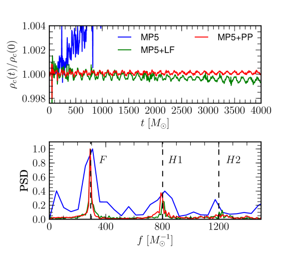
The evolution of the central rest-mass density for the different methods is shown in the top panel of Figure 5. Clearly, the ordinary MP5 prescription shows violent oscillations and a large secular growth. We evolve this model up to time where it has deviations from the initial rest-mass density of the order of . We note that when we have evolved this model using the same prescription as for the test in the Cowling approximation, we have actually obtained even larger oscillations and a more pronounced secular growth leading to an increase of about in the central rest-mass density at time .
As with the previous test, the simple addition of extra numerical dissipation at the star’s surface seems to cure the most severe problems with the MP5 evolution. Indeed the MP5+LF scheme shows much smaller oscillations and only a weak secular trend (see also Figure 1).
The MP5+PP scheme yields very small oscillations and an almost zero trend in the central rest-mass density. However, in preliminary tests the MP5+PP scheme showed a sudden increase in the oscillation amplitude and in the secular drift after time , which were at levels comparable to the MP5+LF ones. The reason for this behaviour is to be found in the prolongation operators used in our AMR setup as well as in the lack of refluxing in our code, which were resulting in spurious violations in the mass conservation at the mesh-refinement boundaries in the low density regions outside of the star. In order to avoid this problem we have disabled the prolongation of the hydrodynamic variables, thus partially “decoupling” the various refinement levels. In the long term we plan to improve the AMR capabilities of our code to avoid these pathologies, but these are not of primary concern for the main purpose of our code, which is to compute gravitational waveforms from compact binaries.
The PSD of the central rest-mass density is shown in the bottom panel of Figure 5. There, we show the PSD normalized to have maximum amplitude of for the different numerical schemes. The spectra are computed using the central rest-mass density from the time , to remove the dependence from the relaxation of the initial data. In order to remove the low-frequency contribution from the secular growth we compute the spectra after removing the secular terms via a linear fit. Clearly, the ordinary MP5 scheme has a more noisy spectrum, partly because of the shorter integration time. Apart from that, all the three methods show spectra which are peaked at the frequencies corresponding to the -mode and to the first overtone, , as computed from linear perturbation theory.
4.3 Nonlinear Oscillations: the Migration Test
The third test that we discuss is the study of the large, nonlinear, oscillations of a TOV migrating from the unstable branch of equilibrium solutions to the stable one. This is a commonly adopted test for numerical-relativity codes, e.g. [41, 50, 24, 51, 52], and has been studied in detail by [53, 54]. Here we consider a model initially described by a polytropic EOS with and and with central rest-mass density , yielding an ADM mass of . The migration is triggered by the use of an outgoing velocity perturbation of the form , where is the areal radius and is chosen so that the maximum perturbation velocity is . The evolution is performed with a Gamma-law equation of state to allow for shock heating. We do not solve the constraints equations after the application of the initial perturbation, but we rely on the constraint-damping nature of CCZ4 to bring the evolution back to the constraint “hypersurface” as done in [55].
The grid setup is identical to the one described in Section 4.2. Here, again, we use the same atmosphere prescription for all the schemes with and we evolve all the models using the SSP RK3 scheme with a CFL of . Finally, the spacetime is evolved using sixth-order finite differencing and with the addition of a fifth-order Kreiss-Oliger dissipation.
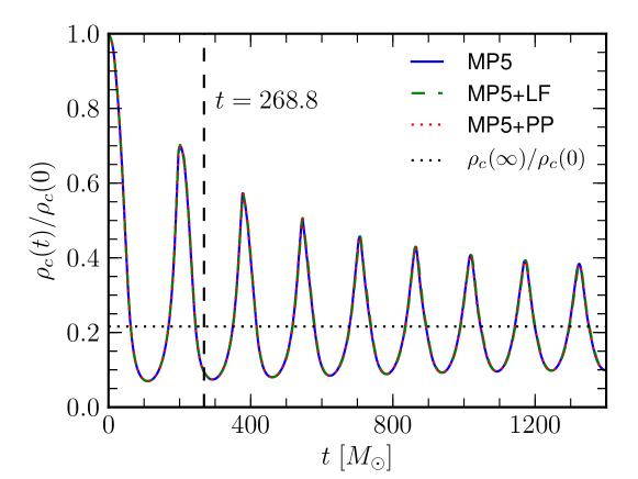
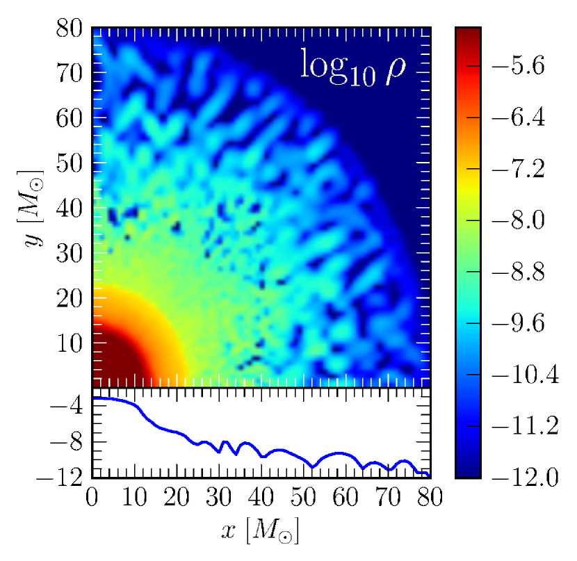
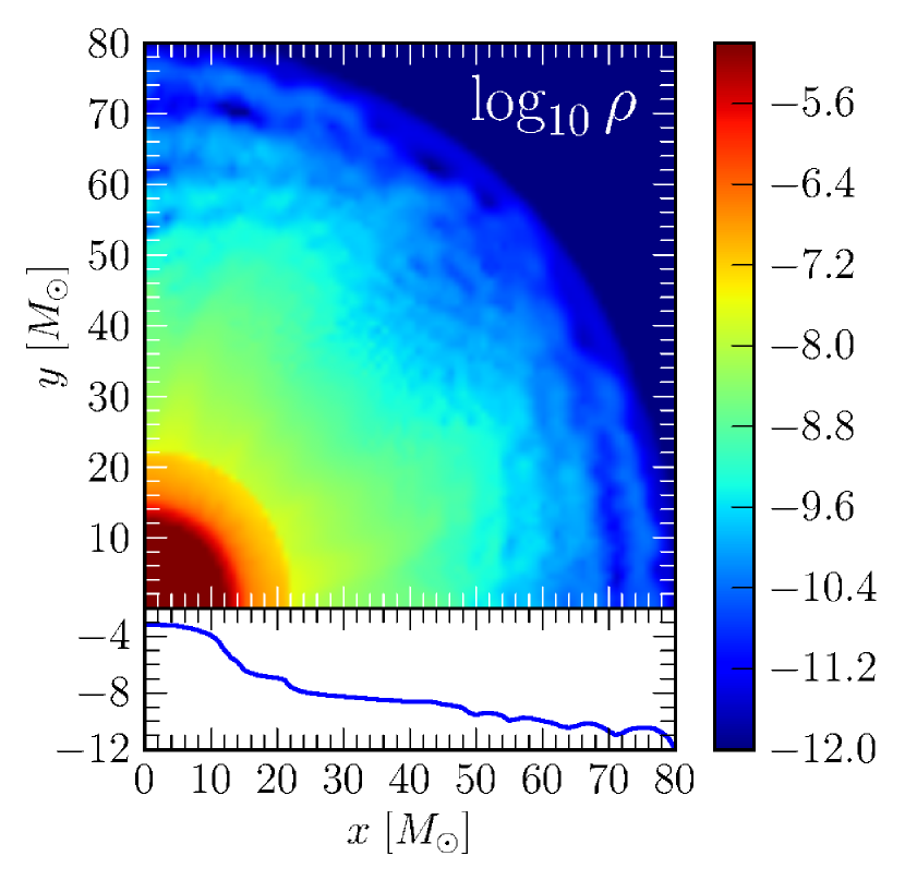
The evolution of the system is summarized by Figure 6, where we show the evolution of the central rest-mass density, normalized to its initial value, for our three different schemes. As can be seen from the figure, the star undergoes a sequence of violent expansion, contraction cycles after it has migrated on the stable branch of equilibria, while conserving the baryonic mass. During the contraction phase, shocks are formed and part of the shock-heated matter is ejected with large velocities from the central object. All of the methods are perfectly adequate for this test and only minimal differences appear between the MP5+LF scheme and the other two in the amplitude of the first peak.
MP5
MP5+LF
MP5+PP
The difference between the various atmosphere prescriptions is better appreciated by looking at Figure 7, where we show a two-dimensional cut of the of the rest-mass density at the time when the matter ejected at the first bounce reaches the grid boundaries (this is indicated with a vertical line in Figure 6). As can be seen from the figure, both MP5 and MP5+PP are able to capture the dynamics of the low-density ejecta without introducing large numerical oscillations or excessive deviations from spherical symmetry. The front of the ejecta is reasonably well captured even if it has crossed two mesh-refinement boundaries, where our code cannot currently ensure mass-conservation and hence the right propagation speed for shocks. On the other hand, the MP5+LF method exhibits large numerical oscillations, which lead to small islands of larger rest-mass density. This is probably due to our choice of avoiding the reconstruction in characteristic variables at low densities, since it is well known that component-by-component reconstruction typically results in oscillatory solutions when used in conjunction with high-order schemes. Of course, given the smallness of the rest mass which is concentrated in these fragments, the bulk dynamics of the matter is essentially unaltered and the spectral properties of the oscillating star are as in the other methods.
4.4 Gravitational Collapse to Black-Hole
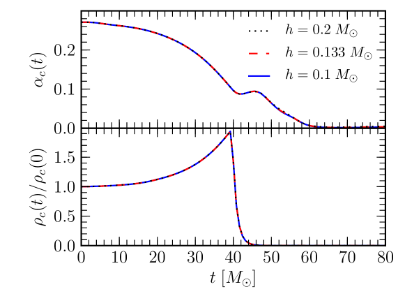
The final test involving isolated neutron stars that we describe is the gravitational collapse of a TOV to a black hole. This is another commonly adopted benchmark for general-relativistic hydrodynamics codes and has been studied in great detail in [56, 57, 58]. The model that we consider here is initially described by a polytropic EOS with and and has an initial central rest-mass density of , yielding an ADM mass of . The collapse is triggered with the addition of a velocity perturbation with the same properties of the one employed in the migration test, but with opposite sign, i.e. an ingoing perturbation. The model is evolved using an Gamma-law EOS to allow for thermal effects.
In the case of the collapse the influence of the atmosphere is negligible, so we consider only evolutions performed with the MP5+LF prescription. As in the migration test, our computational domain covers and we assume reflection symmetry across the and planes. We employ four different refinement levels with the finest one covering the star entirely with diameters and we study the convergence of the code as we vary the resolution. In particular we considered six different resolutions having grid spacing (in the finest refinement level) of respectively. We also perform a higher-resolution run, with , which we evolve only up to time and that we use as a reference solution to measure the self-convergence of the code. We adopt sixth-order finite differencing for the spacetime, which is evolved using the CCZ4 formulation, with fifth-order Kreiss-Oliger artificial dissipation on the metric variables. We use the fourth-order Runge-Kutta scheme as time integrator, so that our scheme is formally fourth-order (fifth-order in space and fourth in time). Finally, in order to avoid excessive oscillations in the matter fields inside the forming black hole, we artificially evacuate the regions where by adding an artificial damping term in the sources of the hydrodynamic variables as done in [59]. We also switch to the component-wise reconstruction with Lax-Friedrichs split in regions where .
The evolution of the lapse and the rest-mass density at the coordinate origin and for the different resolutions are shown in Figure 8. As the star collapses the central rest-mass density rapidly increases and the lapse function approaches zero. At time the lapse at the center becomes smaller than and the rest-mass density starts to be dissipated. Finally, after a small re-bounce, the lapse settles and the evolution reaches quasi-stationarity. The exact behaviour of the lapse is determined by the way in which we evacuate the fluid, since we found that in simulations without matter damping, the lapse showed a smaller bounce at the moment of the collapse, but a more irregular evolution at intermediate times.
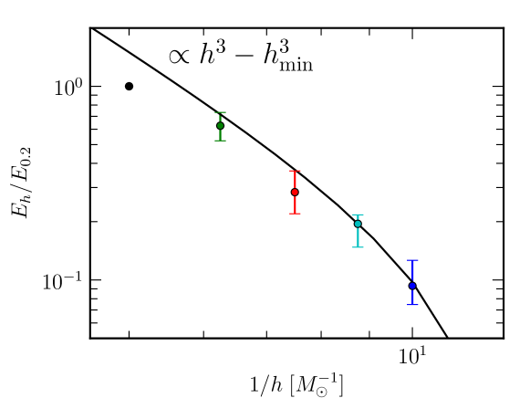
In order to estimate the convergence rate of our code we use the highest resolution simulation, , as a reference solution and we compute the error of a given physical quantity, , at the time as
| (6bc) |
where the sum is taken over the common grid points between the resolution and the highest resolution run on the plane. is then computed using data-sets equally spaced in time the interval (including the first and the last time). In order to have an absolute measure of the relative errors between the different resolutions over the whole time-interval, we normalize the error estimates with respect to the deviations as measured between the lowest resolution simulation and the reference one, i.e. . Finally, we take as relative error the average in time of the normalized error estimates and we use the maximum and minimum relative errors (between the different times) as a measure of the uncertainty of this procedure.
The results obtained for the lapse function are shown in Figure 9. Also shown, as a solid black line, is the curve for third-order convergence. As can be seen from the figure, our data is consistent with third-order convergence for . As commented before, our code is formally fourth-order convergent in time and fifth-order in space, on the other hand, based on our previous experience with MP5 in [8], we argue that the observed third-order convergence is most probably related to the fact that high-order shock-capturing codes are able to converge at their nominal order only at extremely high resolutions. This is due to the fact that their nominal accuracy is typically spoiled by the activation of the flattening procedure close to under resolved features of the solution (see discussion in [8]).
5 Binary Neutron Stars
In this Section we present results obtained for the inspiral and merger of binary neutron stars in quasi-circular orbit. We consider a binary having an initial small separation of , as this binary can be simulated with relatively small computational costs, allowing us to explore the different atmosphere prescriptions and make a detailed comparison between the results obtained with our code and the ones obtained with the original Whisky code. The same binary, but at the larger separation of , has been considered in [1].
We recall here that the Whisky code is a second-order finite-volume code with high-order primitive reconstruction and implements several different approximate Riemann solvers. For the runs presented here we make use of the PPM reconstruction [60] and of the HLLE Riemann solver [61, 62]. We remark that Whisky is a good representative of the current state-of-the-art for numerical general-relativistic hydrodynamics [63].
The initial data is computed in the conformally-flat approximation using the LORENE pseudo-spectral code [64] and is publicly available [65]. The EOS assumed for the initial data is polytropic with and , while the evolution is performed using the Gamma-law EOS to allow for thermal effects in the merger phase. The details of the binaries we consider are listed in Table 2, but it is important to point out that the neutron stars composing these binaries have a rather high baryonic mass, , close to the maximum mass allowed by the EOS for nonrotating models, , and having high compactness, , being the gravitational mass of each of the two stars when at infinite separation and the corresponding areal radius. Binaries with a similar compactness have been already considered in [5], where it was found that high-compactness binaries are much more challenging to evolve accurately with respect to low-compactness ones.
-
Binary A B
-
Run Code Method MOL CFL A.MP5.H1 WhiskyTHC MP5 RK4 0.30 5 0.40000 A.MP5.H2 WhiskyTHC MP5 RK4 0.30 6 0.20000 A.MP5.H4 WhiskyTHC MP5 RK4 0.30 6 0.12800 A.MP5+LF.H2 WhiskyTHC MP5+LF RK4 0.30 6 0.20000 A.MP5+PP.H2 WhiskyTHC MP5+PP RK3 0.15 6 0.20000 A.PPM.H2 Whisky PPM RK4 0.30 6 0.20000 A.PPM.H3 Whisky PPM RK4 0.30 6 0.13333 A.PPM.H5 Whisky PPM RK4 0.30 6 0.10000
In what follows we discuss the results obtained from eight different evolutions of the binary A described in Table 2. As a comparison, in the table we also present the properties of the binary we have considered in [1], i.e. binary B. All of these runs are performed on a grid covering , , where we assume reflection symmetry across the plane and symmetry across the plane. The grid employs several fixed refinement levels, or depending on the run, with the finest refinement levels covering both stars, i.e. we have no moving boxes. The refinement levels have diameters on the equatorial plane of and (the finest one is removed for run A.MP5.H1). A summary of the main numerical parameters can be found in Table 3.
Finally, we evolve this model using the CCZ4 formulation with damping constant and with beta-driver . The spacetime is evolved using fourth-order finite differencing and with fifth-order Kreiss-Oliger artificial dissipation. The evolutions are performed without resetting the shift to zero at the beginning of the simulation, which is known to yield a more oscillatory behaviour in the coordinates [66]. There is no particular reason for this choice: the gauges are only chosen so as to be able to leverage, in the debugging stage, on the comparison with previously existing Whisky simulations that were performed, with a different grid setup, by [59].
Since our focus here is mostly on the accuracy of the calculation of the gravitational radiation from compact neutron-star binaries, we consider the accuracy of the code by mainly looking at the mode of the Weyl scalar extracted at the fixed coordinate radius of (). We do not attempt to extrapolate in radius or compute the strain as this involves other uncertainties [67, 68, 69, 70].
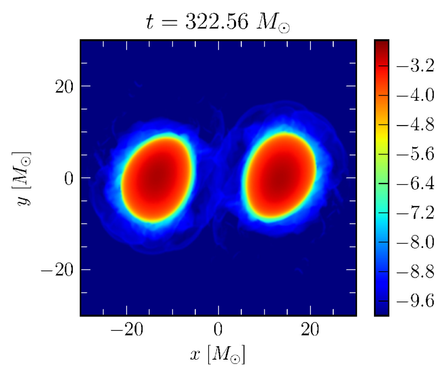
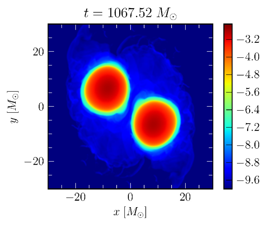
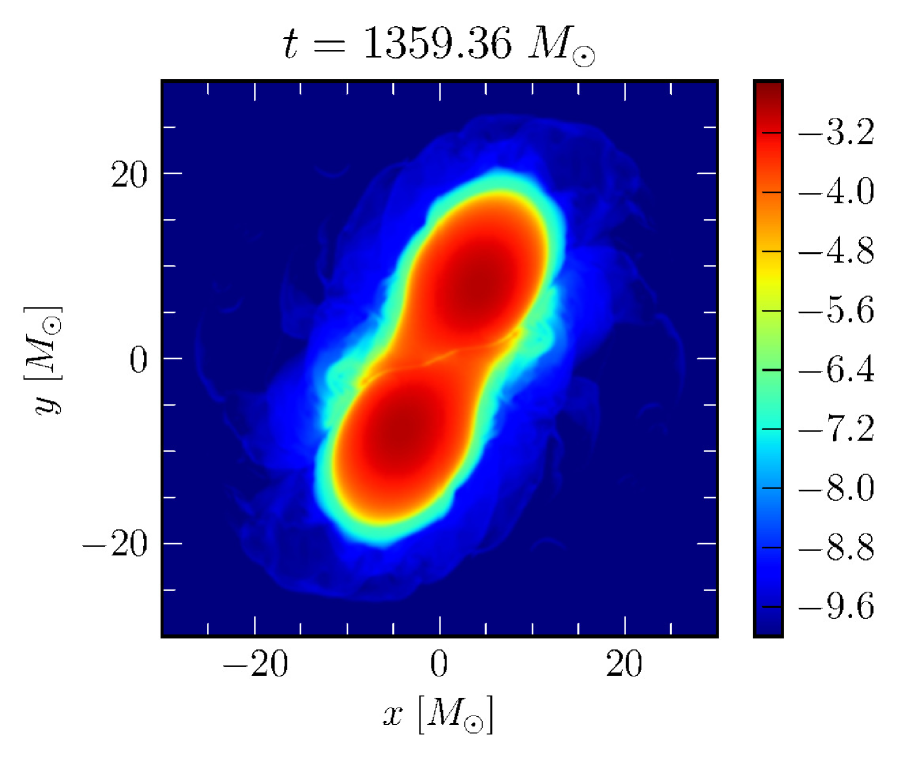
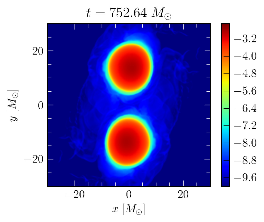
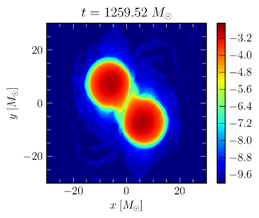
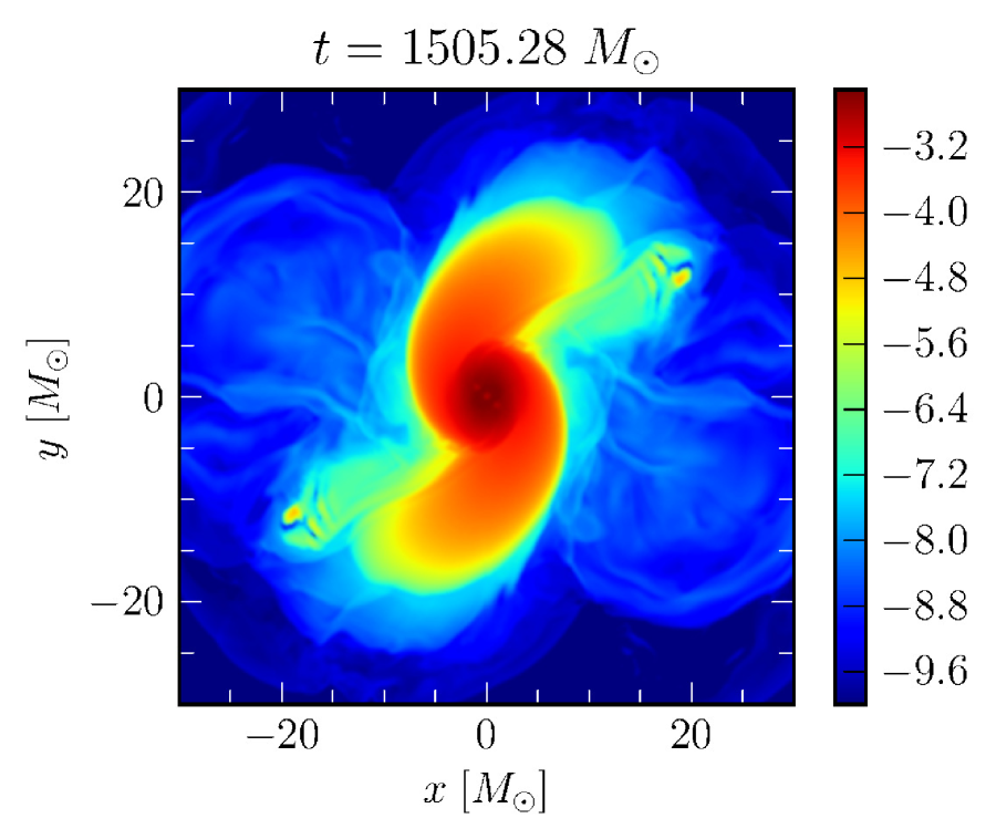
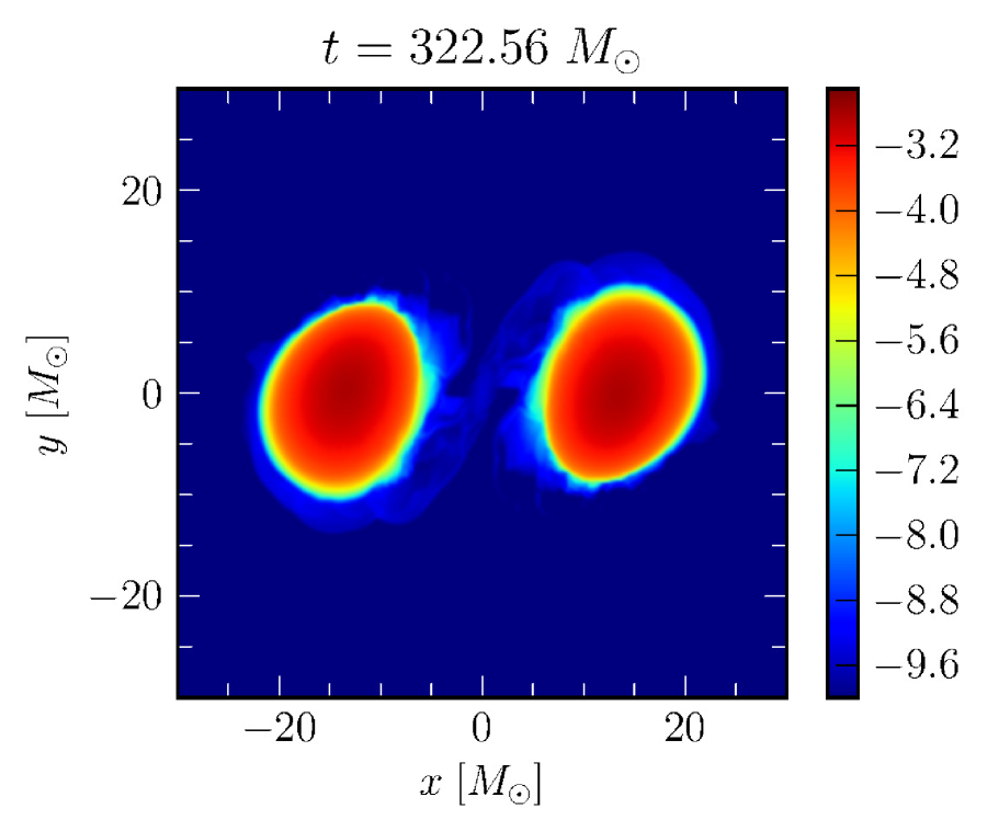
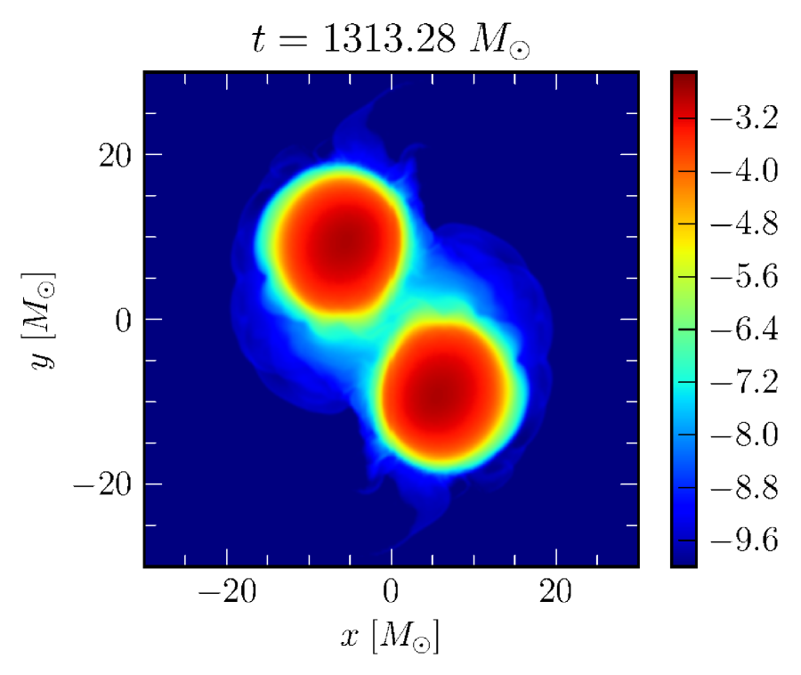
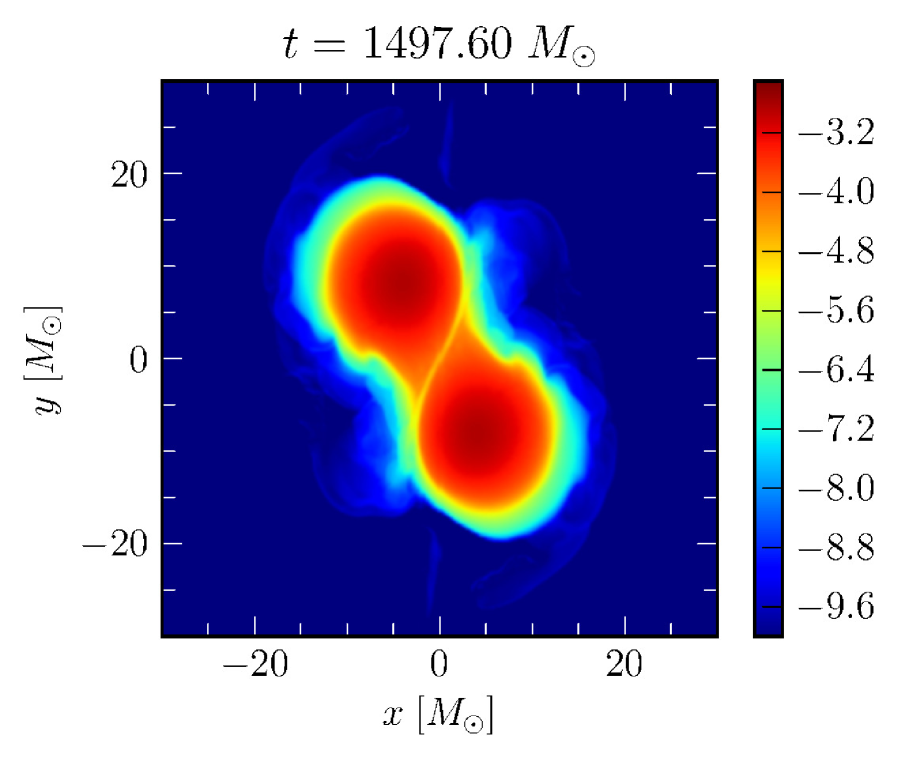
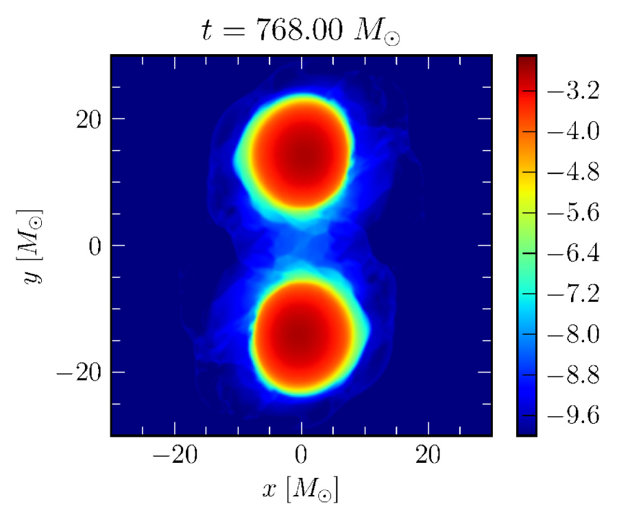
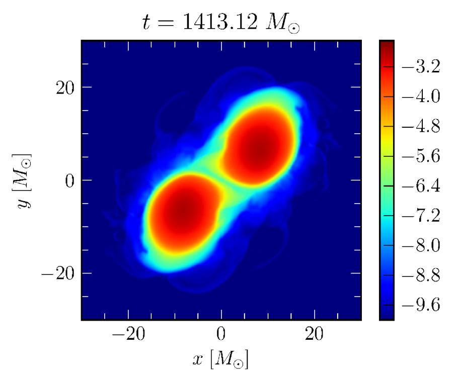
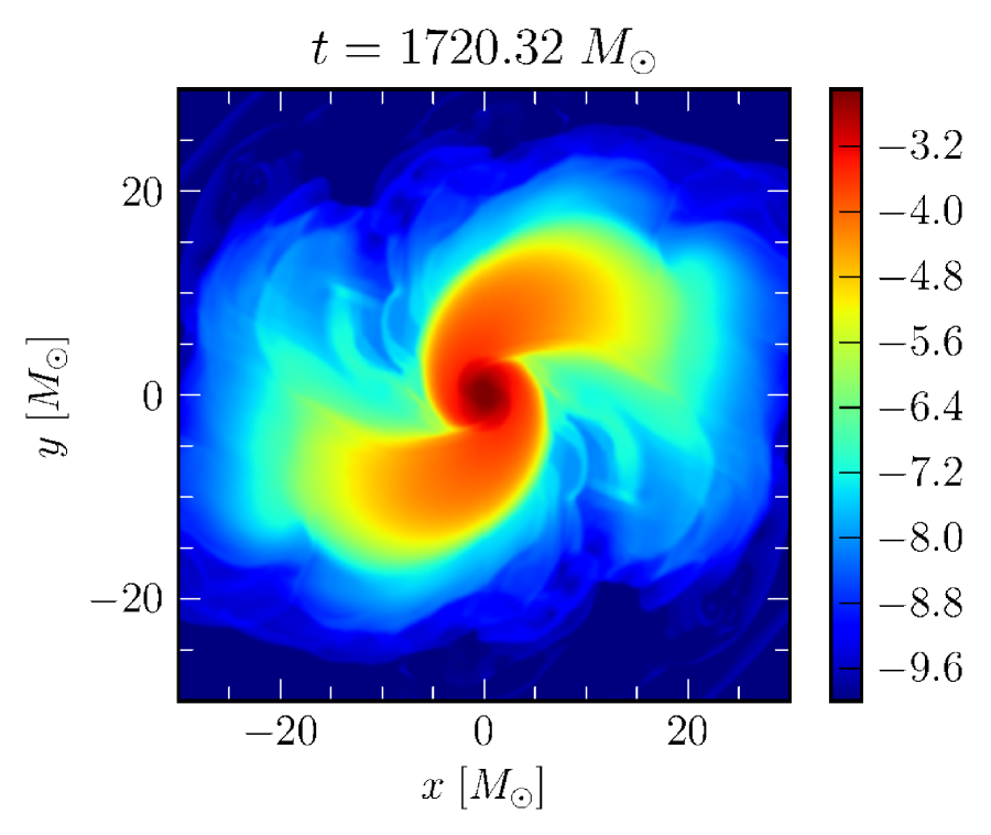
The dynamics of the inspiral and merger of binary neutron stars has been described many times and in great detail in the literature, e.g. [66]; for this reason we do not give a very in-depth discussion of it here. The two neutron stars inspiral for about orbits, touch and quickly merge into a black-hole. For this particular model no significant disk is left behind. The gravitational-wave signal consists of about seven cycles up to merger, followed by the black-hole ringdown.
An overview of the inspiral and merger dynamics is shown in Figures 10 and 11 for the WhiskyTHC and Whisky codes, respectively, at the common resolution of . There we plot the of the rest-mass density on the plane at six representative times. As remarked in [66], the large deformations of the stars is only an apparent one and is due mostly to the large deformation of the coordinates arising from the use of an initially non-zero shift as specified by the LORENE initial data.
From a simple comparison of Figures 10 and 11, it is possible to appreciate that WhiskyTHC is able to preserve the initial sharp profile of the two neutron stars for the whole duration of the inspiral and up to the merger. In comparison, the second-order methods of the original Whisky code result in a significant smearing of the rest-mass density profile. As a consequence, the contact appears to be more smooth in the simulations made with Whisky than with WhiskyTHC and, in particular, with the latter one it is possible to notice the formation of strong shock waves at the moment of the contact that eject, but do not unbind, part of the neutron-star matter in the direction of the separatrix between the two stars (cf. last panel of Figure 10). This is consistent with what described by the toy model proposed in [71] in the case of equal-mass binaries.
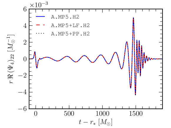
The gravitational-wave signal is shown in Figure 12, where we plot the mode of , as extracted at , and as a function of the retarded time , where . In particular, we show the results obtained for runs A.MP5.H2, A.MP5+LF.H2 and A.MP5+PP.H2, where obviously the three names refer to simulations performed with the MP5, the MP5+LF, and MP5+PP methods, respectively.
As can be seen from the plot, all our three different atmosphere prescriptions give identical results during the inspiral and yield very marginal differences in the merger phase. This provides an important result and suggests that the treatment of the neutron star surface is not a leading source of error in binary-neutron-star simulations, as far as the inspiral gravitational-wave signal is concerned. The particular choice of time-integrator, between SSP-RK3 and the standard RK4, also seems not to be of fundamental importance here, with the error being most likely dominated by the spatial discretization. On the other hand, in order to use the proper positivity-preserving limiter, the timestep used for the A.MP5+PP.H2 run is only half of the one used in the other runs thus possibly introducing a systematic difference.
Whisky
WhiskyTHC
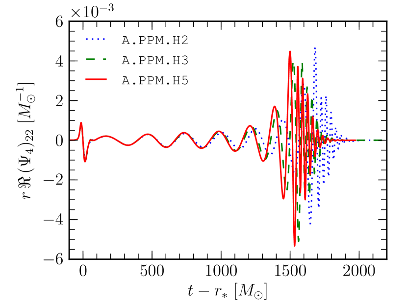
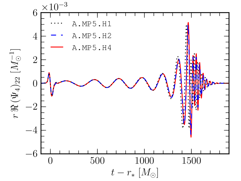
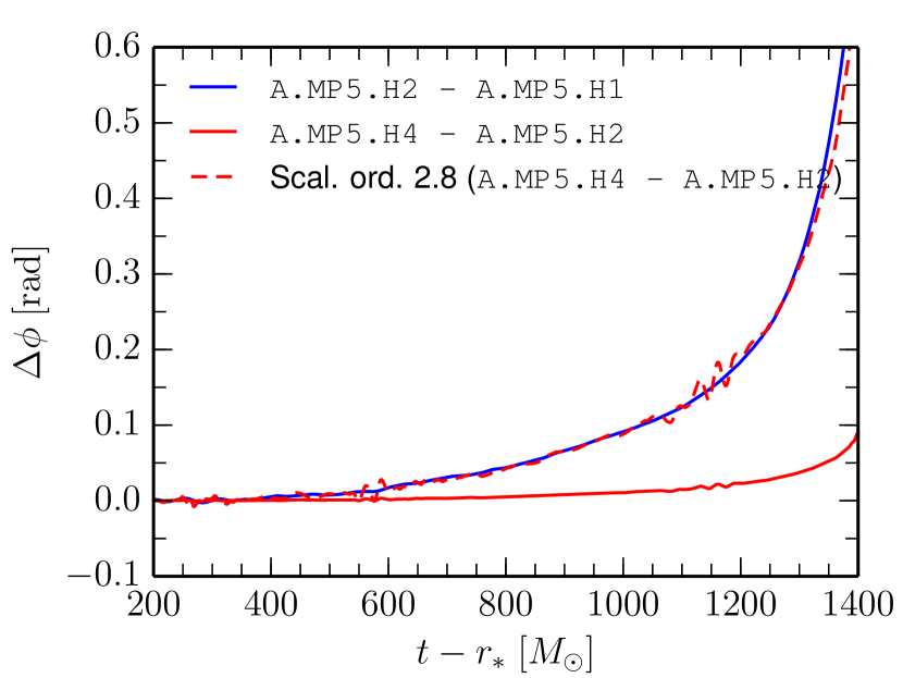
The gravitational-wave signal for the other runs of binary A are shown in Figure 13, where in the left panel we show the results obtained with the standard Whisky code and in the right one those obtained with WhiskyTHC. The first aspect to notice when comparing the two panels is that, when using a second-order code, the phase difference between the gravitational-waves at different resolutions is significant. We can observe a difference between the low and the high resolution of about radians at , with being the extraction radius. In contrast, the waveforms obtained with WhiskyTHC show a significantly smaller de-phasing: the difference between the low and the high resolution is about radians at , which is a factor four smaller than the one shown by Whisky, even though the WhiskyTHC runs span a wider range of resolutions. The difference in phase between the high and the medium-resolution simulation of WhiskyTHC at is as small as radians. The second interesting aspect is that, for this particular binary and with the Whisky code, the merger takes place earlier as we increase the resolution. This is the opposite of what it is observed in other, less compact binaries, e.g. [4], where tidal effects have been found to be amplified at lower resolution, or is shown by the WhiskyTHC code.
Whisky
WhiskyTHC
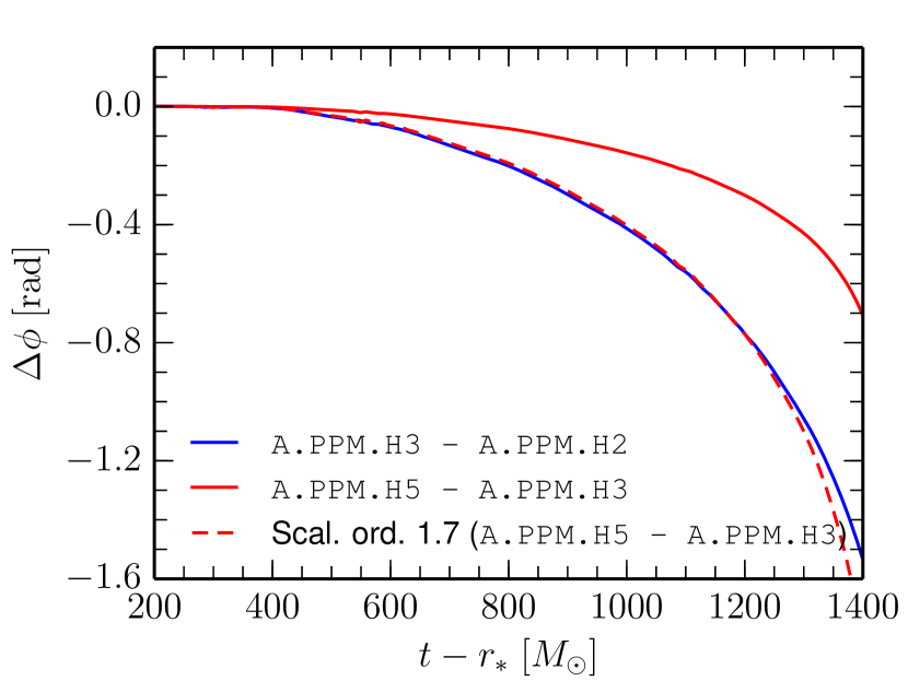
We study the convergence of the waveforms by looking at the de-phasing between different resolutions. For each run we compute the phase, , of the mode of from its definition,
| (6bd) |
over the time interval . Note that we do not align the waveforms at a given time, as done instead in alignment of the waves from different resolutions [3, 5], and which is hard to justify from a mathematical point of view. On the other hand, we exclude from the calculation the first burst of gravitational radiation, due to the initial “junk” radiation present in the initial data. We also exclude the last part of the merger phase (where we expect large errors due to the presence of shock waves) and ringdown, since we are only concerned with the inspiral phase here.
The results are shown in Figure 14, where we measure the convergence rate for both the Whisky and the WhiskyTHC codes. In particular, for Whisky (cf. left panel of Figure 14) we find a convergence order of essentially up to time , i.e. essentially up to the contact time ; this convergence order is comparable with the one reported in [72] and which was . For WhiskyTHC, instead (cf. right panel of Figure 14), we find a convergence order of up to time . It is useful to remark that together with the results reported in [1], where a similar convergence order of was found, this is the first time that higher-than-second-order of convergence has been shown for binary-neutron-star mergers333We note that there are several reasons that could explain why the convergence order found here is slightly smaller than the one found in [1]. The most important among these are that we are considering shorter inspirals here and the CCZ4 formulation that normally requires larger resolutions to enter the convergence regime [17, 59]..
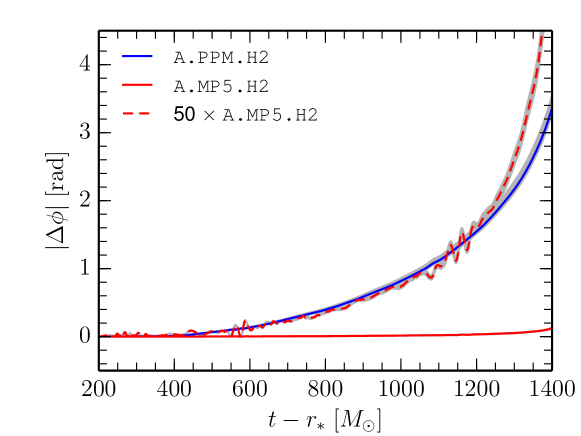
As a consequence of having a higher convergence order, WhiskyTHC is also significantly more accurate. This is shown in Figure 15, where we compare the estimated phase error between the runs A.MP5.H2, A.PPM.H2, and the Richardson extrapolated phase from WhiskyTHC and Whisky, respectively. We roughly estimate the uncertainty in this procedure by performing two different extrapolations for each code, varying the convergence order by with respect to the estimated one. The resulting range of phase errors are shown as shaded regions in the figure. Clearly, the simulation carried out with Whisky has an uncertainty in phase which is almost equivalent to one gravitational-wave cycle, i.e. of the order of of the entire accumulated phase (cf. line A.PPM.H2). At the same time, WhiskyTHC has an error which, at the same resolution and for comparable computational costs, is times smaller than Whisky (cf. A.MP5.H2). We should note that we have also tried to estimate the phase error for WhiskyTHC using the Richardson-extrapolated data obtained with the Whisky code and assuming convergence order of . In this case, we found an even smaller estimated phase error, but with an uncertainty, measured by varying the order in the extrapolation by , of more than . As a final remark, we note that our error estimates only reflect the numerical truncation error. Other systematic errors and, in particular, finite extraction radius effects, inaccuracies in the initial data (e.g. eccentricity) are also present and might be relevant, especially for WhiskyTHC. On the other hand, because we are here interested only in evaluating and comparing the accuracy of the two numerical methods, we can ignore these systematic contributions.
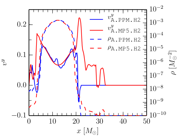
A physical insight on why the Whisky code has a considerably lower accuracy than the WhiskyTHC code can be gained by looking at Figure 16. There, we show one-dimensional cuts of the rest-mass density (solid lines) and of the component of the velocity, , (dashed lines) for runs A.MP5.H2 and A.PPM.H2 along the axis. The data is taken at the approximate time when the first orbit is completed and the centers of the two stars are aligned along the axis. Since this happens at two different times for A.MP5.H2 (blue lines) and A.PPM.H2 (red lines) , the lines in the figure show data taken at two slightly different coordinate times. Particularly important in this comparison is the velocity profile inside the stars, as the velocity in the low-density atmosphere around the stars is in any case dominated by unphysical numerical effects as neither of the two codes is able to provide a reasonable description of the stellar surface. The velocity in the interior, on the other hand, is directly related to the orbital motion of the two stars and hence to the gravitational-wave phase.
As can be seen from the figure, the Whisky code is not able to transport the velocity profile of the star correctly; rather, the higher numerical dissipation has the effect of slowly “flattening” both the rest-mass density and the linear-momentum profiles in the stellar cores. Since this flattening proceeds at different rates for the two different fields, it results in a distortion of the linear velocity profile (and of other related physical quantities), which, in turn, results in a small deformation of the stars. In this case, the artificial deformation is such that the stars become less compact, thus less efficient in losing angular momentum via gravitational waves and hence delaying the time of merger. We expect this deformation to be the leading source of error in the phase evolution for the Whisky code, at least for the high-compactness stars considered here.
6 Conclusions
We have presented a new multi-dimensional, general-relativistic hydrodynamic code, WhiskyTHC, born from the merger of the Whisky and the THC codes. This code inherited from Whisky the primitive recovery routine as well as a new EOS framework with support for composition and energy dependent realistic equation of state [22], and from THC the use of high-order flux-vector splitting finite-differencing schemes [8]. This is the first genuinely higher-than-second-order fully general-relativistic code.
Amongst the new techniques introduced with WhiskyTHC is the use of positivity-preserving limiters [43] as a way to treat low-density regions alternative to the traditional “atmosphere” prescriptions. We have shown that this treatment is able to significantly improve the quality of simulations involving isolated neutron stars and to effectively remove the loss of the conservative properties of the equations in the boundary between the stellar surface and the ambient atmosphere. Because the introduction of positivity preserving limiters in any hydrodynamics code is rather straightforward and allows one to use arbitrarily small values of the atmosphere, we recommend its use as the method of choice for the evolution of compact stars.
We have also demonstrated the accuracy of our code in a series of classical tests involving the linear and nonlinear evolution of isolated neutron stars. In particular, we have shown that our code is able to stably evolve isolated stars for a long time and can attain high order (i.e. third) of convergence in the simulation of the gravitational collapse of nonrotating stars to black holes.
Finally, we have applied our code to the simulation of the late-inspiral and merger of two neutron stars in quasi-circular orbits. Using rather small-separation binaries to test the dependence of the results on the atmosphere treatment, we have shown that our results are completely independent of it. Furthermore, we have demonstrated the higher order of convergence and accuracy of our new code when compared with our old Whisky code, which implements the standard second-order schemes that are commonly employed for matter simulations in numerical relativity. In particular, we have found higher than second-order convergence in the phase and an overall phase error which, at the same resolution and with similar computational costs, is estimated to be times smaller than the one for Whisky for the binaries we considered and at moderate resolution.
Our future plans include the exploitation of the efficiency of the high-order methods in WhiskyTHC to pursue a systematic investigation of tidal effects in binary-neutron-stars mergers, as well as in black-hole neutron star binaries, using realistic equation of states and compactness parameters. We also plan to carefully assess the detectability of such effects by advanced gravitational-wave detectors.
References
References
- [1] Radice D, Rezzolla L and Galeazzi F 2014 Mon. Not. R. Astron. Soc. L. 437 L46–L50 (Preprint 1306.6052)
- [2] Baiotti L, Damour T, Giacomazzo B, Nagar A and Rezzolla L 2010 Phys. Rev. Lett. 105 261101 (Preprint 1009.0521)
- [3] Baiotti L, Damour T, Giacomazzo B, Nagar A and Rezzolla L 2011 Phys. Rev. D 84 024017 (Preprint 1103.3874)
- [4] Bernuzzi S, Nagar A, Thierfelder M and Brügmann B 2012 Phys. Rev. D 86 044030 (Preprint 1205.3403)
- [5] Hotokezaka K, Kyutoku K and Shibata M 2013 Phys. Rev. D 87 044001 (Preprint 1301.3555)
- [6] Aylott B et al. 2009 Class. Quantum Grav. 26 165008 (Preprint 0901.4399)
- [7] Hinder I and et al 2013 Classical and Quantum Gravity 31 025012 (Preprint 1307.5307)
- [8] Radice D and Rezzolla L 2012 Astron. Astrophys. 547 A26 (Preprint 1206.6502)
- [9] Tchekhovskoy A, McKinney J C and Narayan R 2007 Mon. Not. R. Astron. Soc. 379 469–497
- [10] Del Zanna L, Zanotti O, Bucciantini N and Londrillo P 2007 Astron. Astrophys. 473 11–30 (Preprint 0704.3206)
- [11] Bucciantini N and Del Zanna L 2011 Astron. Astrophys. 528 A101 (Preprint 1010.3532)
- [12] Misner C W, Thorne K S and Wheeler J A 1973 Gravitation (San Francisco: W. H. Freeman)
- [13] Rezzolla L and Zanotti O 2013 Relativistic Hydrodynamics (Oxford University Press, Oxford UK)
- [14] Bona C, Bona-Casas C and Palenzuela C 2010 Phys. Rev. D 82 124010 (Preprint 1008.0747)
- [15] Bona C and Palenzuela-Luque C 2005 Elements of Numerical Relativity (Berlin: Springer-Verlag)
- [16] Gundlach C, Martin-Garcia J M, Calabrese G and Hinder I 2005 Classical Quantum Gravity 22 3767–3774 (Preprint gr-qc/0504114)
- [17] Alic D, Bona-Casas C, Bona C, Rezzolla L and Palenzuela C 2012 Phys. Rev. D 85 064040 (Preprint 1106.2254)
- [18] Löffler F, Faber J, Bentivegna E, Bode T, Diener P, Haas R, Hinder I, Mundim B C, Ott C D, Schnetter E, Allen G, Campanelli M and Laguna P 2012 Class. Quantum Grav. 29 115001 (Preprint arXiv:1111.3344[gr-qc])
- [19] http://www.cct.lsu.edu/~eschnett/McLachlan/index.html
- [20] Bona C, Massó J, Seidel E and Stela J 1995 Phys. Rev. Lett. 75 600–603 (Preprint gr-qc/9412071)
- [21] van Meter J R, Baker J G, Koppitz M and Choi D I 2006 Phys. Rev. D 73 124011 (Preprint gr-qc/0605030)
- [22] Galeazzi F, Kastaun W, Rezzolla L and Font J A 2013 Phys. Rev. D 88 064009 (Preprint 1306.4953)
- [23] Banyuls F, Font J A, Ibáñez J M, Martí J M and Miralles J A 1997 Astrophys. J. 476 221
- [24] Baiotti L, Hawke I, Montero P J, Löffler F, Rezzolla L, Stergioulas N, Font J A and Seidel E 2005 Phys. Rev. D 71 024035
- [25] Kreiss H O and Oliger J 1973 Methods for the approximate solution of time dependent problems (Geneva: GARP publication series No. 10)
- [26] Brown D, Diener P, Sarbach O, Schnetter E and Tiglio M 2009 Phys. Rev. D 79 044023 (Preprint 0809.3533)
- [27] Shu C W and Osher S J 1988 J. Comput. Phys. 77 439
- [28] Shu C W 1997 Essentially non-oscillatory and weighted essentially non-oscillatory schemes for hyperbolic conservation laws Lecture notes ICASE Report 97-65; NASA CR-97-206253 NASA Langley Research Center
- [29] Leveque R J 1992 Numerical Methods for Conservation Laws (Basel: Birkhauser Verlag)
- [30] Quirk J 1994 International Journal for Numerical Methods in Fluids 18 555–574
- [31] Anile A M 1990 Relativistic Fluids and Magneto-fluids (Cambridge University Press)
- [32] Font J A 2008 Living Rev. Relativ. 6 4; http://www.livingreviews.org/lrr–2008–7 (Preprint 0704.2608.)
- [33] Schnetter E, Hawley S H and Hawke I 2004 Class. Quantum Grav. 21 1465–1488
- [34] Goodale T, Allen G, Lanfermann G, Massó J, Radke T, Seidel E and Shalf J 2003 Vector and Parallel Processing – VECPAR’2002, 5th International Conference, Lecture Notes in Computer Science (Berlin: Springer)
- [35] Berger M J and Oliger J 1984 J. Comput. Phys. 53 484–512
- [36] Berger M J and Colella P 1989 J. Comput. Phys. 82 64–84
- [37] Reisswig C, Haas R, Ott C D, Abdikamalov E, Mösta P, Pollney D and Schnetter E 2013 Phys. Rev. D 87 064023 (Preprint 1212.1191)
- [38] Galeazzi F 2008 Modelling fluid interfaces in numerical relativistic hydrodynamics Master’s thesis Università degli studi di Padova
- [39] Kastaun W 2006 Phys. Rev. D 74 124024
- [40] Millmore S T and Hawke I 2010 Classical Quantum Gravity 27 015007 (Preprint 0909.4217)
- [41] Font J A, Goodale T, Iyer S, Miller M, Rezzolla L, Seidel E, Stergioulas N, Suen W M and Tobias M 2002 Phys. Rev. D 65 084024 (Preprint gr-qc/0110047)
- [42] Radice D and Rezzolla L 2011 Phys. Rev. D 84 024010 (Preprint 1103.2426)
- [43] Hu X Y, Adams N a and Shu C W 2013 Journal of Computational Physics 242 169–180
- [44] Zhang X and Shu C W 2010 Journal of Computational Physics 229 8918–8934
- [45] Zhang X and Shu C W 2011 Proceedings of the Royal Society A: Mathematical, Physical and Engineering Sciences 467 2752–2776
- [46] Zhang X and Shu C W 2011 Journal of Computational Physics 230 1238–1248
- [47] Balsara D S 2012 Journal of Computational Physics 231 7504–7517
- [48] Tolman R C 1939 Phys. Rev. 55 364
- [49] Oppenheimer J R and Volkoff G 1939 Phys. Rev. 55 374
- [50] Baiotti L, Hawke I, Montero P and Rezzolla L 2003 Computational Astrophysics in Italy: Methods and Tools vol 1 ed Capuzzo-Dolcetta R (Trieste: MSAIt) p 210
- [51] Cordero-Carrión I, Cerdá-Durán P, Dimmelmeier H, Jaramillo J L, Novak J and Gourgoulhon E 2009 Phys. Rev. D 79 024017 (Preprint 0809.2325)
- [52] Thierfelder M, Bernuzzi S and Brügmann B 2011 Phys. Rev. D 84 1–30
- [53] Liebling S L, Lehner L, Neilsen D and Palenzuela C 2010 Phys. Rev. D 81 124023 (Preprint 1001.0575)
- [54] Radice D, Rezzolla L and Kellerman T 2010 Classical Quantum Gravity 27 235015 (Preprint 1007.2809)
- [55] Kastaun W, Galeazzi F, Alic D, Rezzolla L and Font J A 2013 Phys. Rev. D 88 021501 (Preprint 1301.7348)
- [56] Baiotti L and Rezzolla L 2006 Phys. Rev. Lett. 97 141101 (Preprint gr-qc/0608113)
- [57] Baiotti L, Hawke I and Rezzolla L 2007 Classical Quantum Gravity 24 S187–S206 (Preprint gr-qc/0701043)
- [58] Thierfelder M, Bernuzzi S, Hilditch D, Bruegmann B and Rezzolla L 2010 Phys. Rev. D 83 064022 (Preprint 1012.3703)
- [59] Alic D, Kastaun W and Rezzolla L 2013 Phys. Rev. D 88 064049 (Preprint 1307.7391)
- [60] Colella P and Woodward P R 1984 J. Comput. Phys. 54 174
- [61] Harten A, Lax P D and van Leer B 1983 SIAM Rev. 25 35
- [62] Einfeldt B 1988 SIAM J. Numer. Anal. 25 294–318
- [63] Baiotti L, Shibata M and Yamamoto T 2010 Phys. Rev. D 82 064015 (Preprint 1007.1754)
- [64] Gourgoulhon E, Grandclément P, Taniguchi K, Marck J A and Bonazzola S 2001 Phys. Rev. D 63 064029
- [65] http://www.lorene.obspm.fr
- [66] Baiotti L, Giacomazzo B and Rezzolla L 2008 Phys. Rev. D 78 084033 (Preprint 0804.0594)
- [67] Boyle M and Mroué A H 2009 Phys. Rev. D 80 124045 (Preprint 0905.3177)
- [68] Reisswig C, Bishop N T, Pollney D and Szilagyi B 2009 Phys. Rev. Lett. 103 221101 (Preprint 0907.2637)
- [69] Reisswig C, Bishop N T, Pollney D and Szilagyi B 2010 Class. Quantum Grav. 27 075014 (Preprint arXiv:0912.1285)
- [70] Reisswig C and D P 2011 Class. Quantum Grav. 28 195015 (Preprint 1006.1632)
- [71] Kyutoku K, Ioka K and Shibata M 2013 Mon. Not. R. Astron. Soc. L. 437 L6–L10
- [72] Baiotti L, Giacomazzo B and Rezzolla L 2009 Class. Quantum Grav. 26 114005 (Preprint 0901.4955)