Extrapolating gravitational-wave data from numerical simulations
Abstract
Two complementary techniques are developed for obtaining the asymptotic form of gravitational-wave data at large radii from numerical simulations, in the form of easily implemented algorithms. It is shown that, without extrapolation, near-field effects produce errors in extracted waveforms that can significantly affect LIGO data analysis. The extrapolation techniques are discussed in the context of Newman–Penrose data applied to extrapolation of waveforms from an equal-mass, nonspinning black-hole binary simulation. The results of the two methods are shown to agree within error estimates. The various benefits and deficiencies of the methods are discussed.
pacs:
04.25.dg, 04.25.Nx, 04.30.-w, 04.30.DbI Introduction
As numerical simulations of black-hole binaries improve, the criterion for success moves past the ability of a code to merely persist through many orbits of inspiral, merger, and ringdown. Accuracy becomes the goal, as related work in astrophysics and analysis of data from gravitational-wave detectors begins to rely more heavily on results from numerical relativity. One of the most important challenges in the field today is to find and eliminate systematic errors that could pollute results built on numerics. Though there are many possible sources of such error, one stands out as being particularly easy to manage and—as we show—a particularly large effect: the error made by extracting gravitational waveforms from a simulation at finite radius, and treating these waveforms as though they were the asymptotic form of the radiation.
The desired waveform is the one to which post-Newtonian approximations aspire, and the one sought by gravitational-wave observatories: the asymptotic waveform. This is the waveform as it is at distances of over from the system generating the waves. In typical numerical simulations, data extraction takes place at a distance of order from the black holes. At this radius, the waves are still rapidly changing because of real physical effects. Near-field effects Teukolsky (1982); Boyle (2008, 2010) are plainly evident, scaling with powers of the ratio of the reduced wavelength to the radius, .111We use the standard notation . Extraction methods aiming to eliminate the influence of gauge effects alone (e.g., improved Regge–Wheeler–Zerilli or quasi-Kinnersley techniques) will not be able to account for these physical changes.
Even using a rather naive, gauge-dependent extraction method, near-field effects dominate the error in extracted waves throughout the inspiral for the data presented in this paper Boyle (2008). For extraction at , these effects can account for a cumulative error of roughly in amplitude or a phase difference of more than one radian, from beginning to end of a 16-orbit equal-mass binary merger. Note that near-field effects should be proportional to—at leading order—the ratio of in phase and in amplitude, as has been observed previously Hannam et al. (2008); Boyle (2008). Crucially, because the wavelength changes most rapidly during the merger, the amplitude and phase differences due to near-field effects also change most rapidly during merger. This means that coherence is lost between the inspiral and merger/ringdown segments of the waveform.
We can see the importance of this decoherence by looking at its effect on the matched-filtering technique frequently used to analyze data from gravitational-wave detectors. Matched filtering Finn (1992); Finn and Chernoff (1993); Boyle et al. (2009) compares two signals, and . It does this by Fourier transforming each into the frequency domain, taking the product of the signals, weighting each inversely by the noise—which is a function of frequency—and integrating over all frequencies. This match is optimized over the time and phase offsets of the input waveforms. For appropriately normalized waveforms, the result is a number between 0 and 1, denoted , with 0 representing no match, and 1 representing a perfect match. If we take the extrapolated waveform as and the waveform extracted at finite radius as , we can evaluate the match between them. If the extrapolated waveform accurately represents the “true” physical waveform, the mismatch (defined as ) shows us the loss of signal in data analysis if we were to use the finite-radius waveforms to search for physical waveforms in detector data.
The waveforms have a simple scaling with the total mass of the system, which sets their frequency scale relative to the noise present in the detector. In Figs. 1 and 2, we show mismatches between finite-radius and extrapolated data from the Caltech–Cornell group for a range of masses of interest to LIGO data analysis, using the Initial- and Advanced-LIGO noise curves, respectively, to weight the matches. The value of denotes the coordinate radius of extraction for the finite-radius waveform.
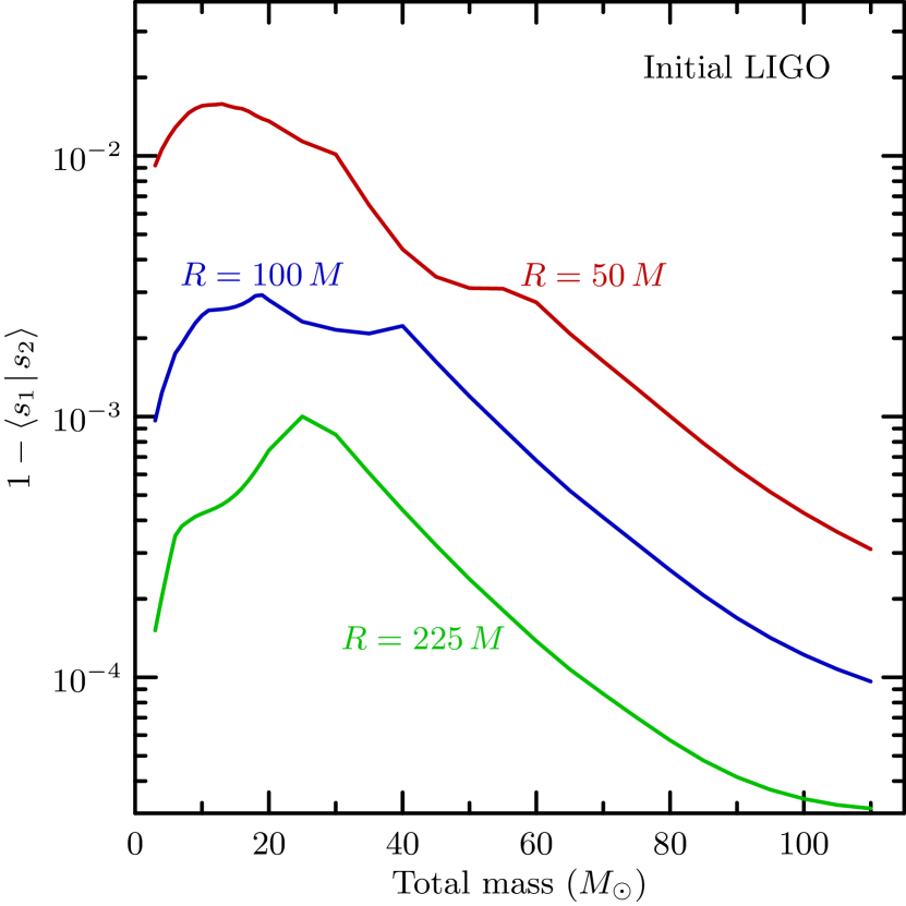
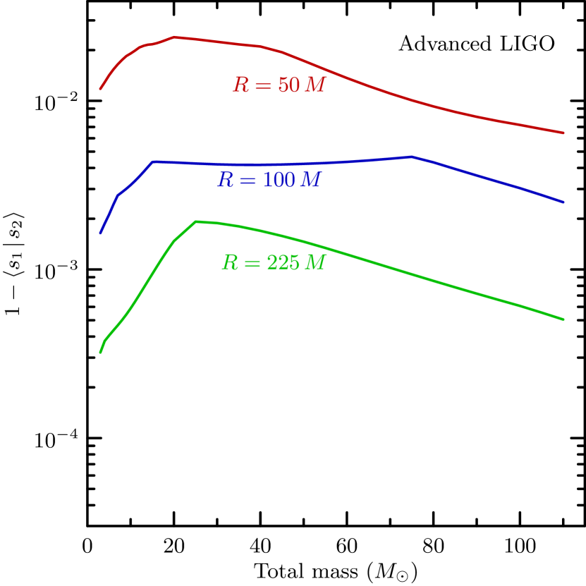
The data in these figures is exclusively numerical data from the simulation used throughout this paper, with no direct contributions from post-Newtonian (PN) waveforms. However, to reduce “turn-on” artifacts in the Fourier transforms, we have simply attached PN waveforms to the earliest parts of the time-domain waveforms, performed the Fourier transform, and set to zero all data at frequencies for which PN data are used. The match integrals are performed over the intersection of the frequencies present in each waveform, as in Ref. Hannam et al. (2009).
This means that the data used here is not truly complete for masses below in Initial LIGO and in Advanced LIGO, and that a detected signal would actually be dominated by data at lower frequencies than are present in this data for masses below about . These masses are correspondingly larger for shorter waveforms, which begin at higher frequencies. It is important to remember that this type of comparison can only show that a given waveform (of a given length) is as good as it needs to be for a detector. If the waveform does not cover the sensitive band of the detector, the detection signal-to-noise ratio would presumably improve given a comparably accurate waveform of greater duration. Thus, the bar is raised for longer waveforms, and for lower masses.
These figures demonstrate that the mismatch can be of order when extracting at a radius of . For extraction at , the mismatch is never more than about . The loss in event rate would be—assuming homogeneous distribution of events in space—roughly 3 times the mismatch when using a template bank based on imperfect waveforms Brown (2004). Lindblom et al. Lindblom et al. (2008) cite a target mismatch of less than between the physical waveform and a class of model templates to be used for detection of events in current LIGO detector data.222 This number of 0.5% results from assumptions about typical event magnitude, template bank parameters, and requirements on the maximum frequency of missed events. The parameters used to arrive at this number are typical for Initial LIGO. Thus, for example, if these numerical waveforms were to be used in construction of template banks,333 We emphasize that these waveforms do not cover the sensitive band of current detectors, and thus would not likely be used to construct template banks without the aid of post-Newtonian extensions of the data. Longer templates effectively have more stringent accuracy requirements, so the suitability of these extraction radii would change for waveforms of different lengths. In particular, our results are consistent with those of Ref. Hannam et al. (2009), which included non-extrapolated data of shorter duration. the waveform extracted at would not be entirely sufficient, in the sense that a template bank built on waveforms with this level of inaccuracy would lead to an unacceptably high reduction of event rate. The waveforms extracted at and , on the other hand, may be acceptable for Initial LIGO. For the loudest signals expected to be seen by Advanced LIGO, the required mismatch may be roughly Lindblom et al. (2008). In this case, even extraction at would be insufficient; some method must be used to obtain the asymptotic waveform. For both Initial and Advanced LIGO, estimating the parameters of the waveform—masses and spins of the black holes, for instance—requires still greater accuracy.
Extrapolation of certain quantities has been used for some time in numerical relativity. Even papers announcing the first successful black-hole binary evolutions Buonanno et al. (2007); Campanelli et al. (2006); Baker et al. (2006) showed radial extrapolation of scalar physical quantities—radiated energy and angular momentum. But waveforms reported in the literature have not always been extrapolated. For certain purposes, this is acceptable—extrapolation simply removes one of many errors. If the precision required for a given purpose allows it, extrapolation is unnecessary. However, for the purposes of LIGO data analysis, we see that extrapolation of the waveform may be very important.
We can identify three main obstacles to obtaining the asymptotic form of gravitational-wave data from numerical simulations:
-
1.
Getting the “right” data at any given point, independent of gauge effects (e.g., using quasi-Kinnersley techniques and improved Regge–Wheeler–Zerilli techniques);
-
2.
Removing near-field effects;
-
3.
Extracting data along a physically relevant path.
Many groups have attempted to deal with the first of these problems.444See Nerozzi et al. (2005) and Sarbach and Tiglio (2001) and references therein for descriptions of quasi-Kinnersley and RWZ methods, respectively. Also, an interesting discussion of RWZ methods, and the possibility of finding the “exact” waveform at finite distances is found in Pazos et al. (2007). While this is, no doubt, an important objective, even the best extraction technique to date is imperfect at finite radii. Moreover, at finite distances from the source, gravitational waves continue to undergo real physical changes as they move away from the system Thorne (1980), which are frequently ignored in the literature. Some extraction techniques have been introduced that attempt to incorporate corrections for these physical near-field effects Abrahams and Evans (1988, 1990); Deadman and Stewart (2009). However, these require assumptions about the form of those corrections, which we prefer not to impose. Finally, even if we have the optimal data at each point in our spacetime, it is easy to see that extraction along an arbitrary (timelike) path through that spacetime could produce a nearly arbitrary waveform, bearing no resemblance to a waveform that could be observed in a nearly inertial detector. In particular, if our extraction point is chosen at a specific coordinate location, gauge effects could make that extraction point correspond to a physical path which would not represent any real detector’s motion. It is not clear how to estimate the uncertainty this effect would introduce to the waveforms, except by removing the effect entirely.
We propose a simple method using existing data-extraction techniques which should be able to overcome each of these three obstacles, given certain very basic assumptions. The data are to be extracted at a series of radii—either on a series of concentric spheres, or at various radii along an outgoing null ray. These data can then be expressed as functions of extraction radius and retarded time using either of two simple methods we describe. For each value of retarded time, the waveforms can then be fit to a polynomial in inverse powers of the extraction radius. The asymptotic waveform is simply the first nonzero term in the polynomial. Though this method also incorporates certain assumptions, they amount to assuming that the data behave as radially propagating waves, and that the metric itself is asymptotically Minkowski in the coordinates chosen for the simulation.
Extrapolation is, by its very nature, a dangerous procedure. The final result may be numerically unstable, in the sense that it will fail to converge as the order of the extrapolating polynomial is increased. This is to be expected, as the size of the effects to be removed eventually falls below the size of noise in the waveform data. There are likely better methods of determining the asymptotic form of gravitational waves produced by numerical simulations. For example, characteristic evolution is a promising technique that may become common in the near future Bishop et al. (1996); Hübner (2001); Babiuc et al. (2005, 2009). Nonetheless, extrapolation does provide a rough and ready technique which can easily be implemented by numerical-relativity groups using existing frameworks.
This paper presents a simple method for implementing the extrapolation of gravitational-wave data from numerical simulations, and the motivation for doing so. In Sec. II, we begin by introducing an extrapolation method that uses approximate tortoise coordinates, which is the basic method used to extrapolate data in various papers Boyle et al. (2007, 2008); Scheel et al. (2009); Boyle et al. (2009); Buonanno et al. (2009) by the Caltech–Cornell collaboration. The method is tested on the inspiral, merger, and ringdown waveform data of the equal mass, nonspinning, quasicircular 15-orbit binary simulation of the Caltech–Cornell collaboration. We present the convergence of the wave phase and amplitude as the extrapolation order increases, and we also compare data extrapolated using various extraction radii. In Sec. III, we propose a different extrapolation method using the wave phase—similar to the method introduced in Ref. Hannam et al. (2008)—to independently check our results, again demonstrating the convergence properties of the method. In Sec. IV, we compare the extrapolated waveforms of both methods at various extrapolation orders, showing that they agree to well within the error estimates of the two methods. A brief discussion of the pitfalls and future of extrapolation is found in Sec. V. Finally, we include a brief appendix on techniques for filtering noisy data, which is particularly relevant here because extrapolation amplifies noise.
II Extrapolation using approximate tortoise coordinates
There are many types of data that can be extracted from a numerical simulation of an isolated source of gravitational waves. The two most common methods of extracting gravitational waveforms involve using the Newman–Penrose quantity, or the metric perturbation extracted using Regge–Wheeler–Zerilli techniques. Even if we focus on a particular type of waveform, the data can be extracted at a series of points along the axis, for example, or decomposed into multipole components and extracted on a series of spheres around the source. To simplify this introductory discussion of extrapolation, we ignore the variety of particular types of waveform data. Rather, we generalize to some abstract quantity , which encapsulates the quantity to be extrapolated and behaves roughly as a radially outgoing wave.
We assume that travels along outgoing null cones, which we parametrize by a retarded time . Along each of these null cones, we further assume that can be expressed as a convergent (or at least asymptotic) series in —where is some radial coordinate—for all radii of interest. That is, we assume
| (1) |
for some functions . The asymptotic behavior of is given by the lowest nonzero .555For example, if , then gives the asymptotic behavior; if , then gives the asymptotic behavior.
Given data for such an at a set of retarded times, and a set of radii , it is a simple matter to fit the data for each value of to a polynomial in . That is, for each value of , we take the set of data and fit it to a finite polynomial so that
| (2) |
Standard algorithms Press et al. (2007) can be used to accomplish this fitting; here we use the least-squares method. Of course, because we are truncating the series of Eq. (1) at , some of the effects from terms will appear at lower orders. We will need to choose appropriately, checking that the extrapolated quantity has converged sufficiently with respect to this order.
II.1 Radial parameter
One subtlety to be considered is the choice of parameter to be used in the extraction and fitting. For numerical simulation of an isolated system, one simple and obvious choice is the coordinate radius used in the simulation. Alternatively, if the data is measured on some spheroidal surface, it is possible to define an areal radius by measuring the area of the sphere along with , and setting . Still other choices are certainly possible.
One objective in choosing a particular parameter is to ensure the physical relevance of the final extrapolated quantity. If we try to detect the wave, for example, we may want to think of the detector as being located at some constant value of . Or, we may want to asymptotically represent the luminosity distance. These conditions may be checked by inspecting the asymptotic behavior of the metric components in the given coordinates. For example, if the metric components in a coordinate system including asymptotically approach those of the standard Minkowski metric, it is not hard to see that an inertial detector could follow a path of constant parameter.
Suppose we have two different parameters and which can be related by a series expansion
| (3) |
For the data presented in this paper, we can show that the coordinate radius and areal radius are related in this way. Introducing the expansion coefficients , we can write
| (4) |
Inserting Eq. (3) into this formula, Taylor expanding, and equating terms of equal order , shows that and . Thus, if the asymptotic behavior of is given by or , the final extrapolated data should not depend on whether or is used. On the other hand, in practice we truncate these series at finite order. This means that higher-order terms could “pollute” or . The second objective in choosing an parameter, then, is to ensure fast convergence of the series in Eq. (2). If the extrapolated quantity does not converge quickly as the order of the extrapolating polynomial is increased, it may be due to a poor choice of parameter.
The coordinate radius used in a simulation may be subject to large gauge variations that are physically irrelevant, and hence are not reflected in the wave’s behavior. That is, the wave may not fall off nicely in inverse powers of that coordinate radius. For the data discussed later in this paper, we find that using the coordinate radius of extraction spheres is indeed a poor choice, while using the areal radius of those extraction spheres improves the convergence of the extrapolation.
II.2 Retarded-time parameter
Similar considerations must be made for the choice of retarded-time parameter to be used in extrapolation. It may be possible to evolve null geodesics in numerical simulations, and use these to define the null curves on which data is to be extracted. While this is an interesting possibility that deserves investigation, we propose two simpler methods here based on an approximate retarded time constructed using the coordinates of the numerical simulation and the phase of the waves measured in that coordinate system.
Again, we have two criteria for choosing a retarded-time parameter. First is the physical suitability in the asymptotic limit. For example, we might want the asymptotic to be (up to an additive term constant in time) the proper time along the path of a detector located at constant . Again, checking the asymptotic behavior of the metric components with respect to and should be a sufficient test of the physical relevance of the parameters. Second, we wish to have rapid convergence of the extrapolation series using the chosen parameter, which also needs to be checked.
As before, we can also show the equivalence of different choices for the parameter. Suppose we have two different approximations and that can be related by a series expansion
| (5) |
Using the new expansion coefficients , we can write
| (6) |
Now, however, we need to assume that the functions can be well-approximated by Taylor series. If this is true, we can again show that or, if we have , that . The condition that be well-approximated by a Taylor series is nontrivial, and can help to inform the choice of . Similarly, the speed of convergence of the extrapolation can help to inform the choice of a particular parameter. While it has been shown Damour et al. (2008) that a retarded-time parameter as simple as is sufficient for some purposes, we find that convergence during and after merger is drastically improved when using a somewhat more careful choice.
Since we will be considering radiation from an isolated compact source, our basic model for comes from the Schwarzschild spacetime; we assume that the system in question approaches this spacetime at increasing distance. In analogy with the time-retardation effect on outgoing null rays in a Schwarzschild spacetime Chandrasekhar (1992), we define a “tortoise coordinate” by:
| (7) |
where is the ADM mass of the initial data.666 Kocsis and Loeb Kocsis and Loeb (2007) pointed out that the propagation of a roughly spherical gravitational wave should be affected primarily by the amount of mass interior to the wave. Because the waves from a merging binary can carry off a significant fraction (typically a few percent) of the binary’s mass, this suggests that we should allow the mass in this formula to vary in time, falling by perhaps a few percent over the duration of the waveform. However, this is a small correction of a small correction; we have not found it necessary. Perhaps with more refined methods, this additional correction would be relevant. In standard Schwarzschild coordinates, the appropriate retarded time would be given by . It is not hard to see that the exterior derivative is null with respect to the Schwarzschild metric.
Taking inspiration from this, we can attempt to account for certain differences from a Schwarzschild background. Let and denote the simulation’s coordinates, and suppose that we extract the metric components , , and from the simulation. We seek a such that
| (8) |
is null with respect to these metric components. That is, we seek a such that
| (9) |
We introduce the ansatz , where is assumed to be a slowly varying function of ,777More specifically, we need . This condition needs to be checked for all radii used, at all times in the simulation. For the data presented below, we have checked this, and shown it to be a valid assumption, at the radii used for extrapolation. and is given by Eq. (7) with in place of on the right side. If we ignore and insert our ansatz into Eq. (9), we have
| (10) |
We can solve this for :
| (11) |
Substituting the Schwarzschild metric components shows that we should choose the negative sign in the numerator of the second factor. Finally, we can integrate (numerically) to find
| (12) |
Now, in the case where is small compared to 1, we may wish to ignore it, in which case we have
| (13) |
It is not hard to see that this correctly reduces to in the Schwarzschild case.
For the data discussed later in this paper, we make further assumptions that , and that . That is, we define the corrected time
| (14a) | |||
| and the retarded time | |||
| (14b) | |||
We find that this corrected time leads to a significant improvement over the naive choice of , while no improvement results from using Eq. (12).
II.3 Application to a binary inspiral
To begin the extrapolation procedure, we extract the (spin-weight ) component of data on a set of spheres at constant coordinate radius in the simulation.888See Ref. Scheel et al. (2009) for details of the extraction procedure. We use data here, rather than Regge–Wheeler–Zerilli data because the data from this simulation is of higher quality; it appears that the RWZ data is more sensitive to changes in gauge conditions after the merger. This problem is still under investigation. In the black-hole binary simulations used here (the same as those discussed in Refs. Boyle et al. (2007); Boyle (2008); Boyle et al. (2008); Scheel et al. (2009)), these spheres are located roughly999 Explicitly, the extraction spheres are at radii , though we find that the final result is not sensitive to the exact placement of the extraction spheres. every (where is the sum of the irreducible masses of the black holes in the initial data) from an inner radius of to an outer radius of , where denotes the total apparent-horizon mass of the two holes at the beginning of the simulation. This extraction occurs at time steps of throughout the simulation. We also measure the areal radius, , of these spheres by integrating the induced area element over the sphere to find the area, and defining . This typically differs from the coordinate radius by roughly . Because of gauge effects, the areal radius of a coordinate sphere changes as a function of time, so we measure this as a function of time. Finally, we measure the average value of as a function of coordinate time on the extraction spheres to correct for the dynamic lapse function. The areal radius and are then used to compute the retarded time defined in Eq. (14).
The gravitational-wave data , the areal radius , and the lapse are all measured as functions of the code coordinates and . We can use these to construct the retarded time defined in Eq. (14), using in place of . This, then, will also be a function of the code coordinates. The mapping between and is invertible, so we can rewrite as a function of and .
As noted in Sec. II.2, we need to assume that the extrapolated functions are well approximated by Taylor series. Because the real and imaginary parts of are rapidly oscillating in the data presented here, we prefer to use the same data in smoother form. We define the complex amplitude and phase of the wave:
| (15) |
where and are functions of and . Note that this definition factors out the dominant behavior of the amplitude. This equation defines the phase with an ambiguity of multiples of . In practice, we ensure that the phase is continuous as a function of time by adding suitable multiples of . The continuous phase is easier to work with for practical reasons, and is certainly much better approximated by a Taylor series, as required by the argument surrounding Eq. (6).
A slight complication arises in the relative phase offset between successive radii. Noise in the early parts of the waveform makes the overall phase offset go through multiples of essentially randomly. We choose some fairly noise-free (retarded) time and ensure that phases corresponding to successive extraction spheres are matched at that time, by simply adding multiples of to the phase of the entire waveform—that is, we add a multiple of to the phase at all times.
Extrapolation of the waveform, then, basically consists of finding the asymptotic forms of these functions, and as functions of time. We apply the general technique discussed above to and . Explicitly, we fit the data to polynomials in for each value of retarded time:
| (16a) | ||||
| (16b) | ||||
The asymptotic waveform is fully described by and . When the order of the approximating polynomials is important, we will denote by and the asymptotic waveforms resulting from approximations using polynomials of order .
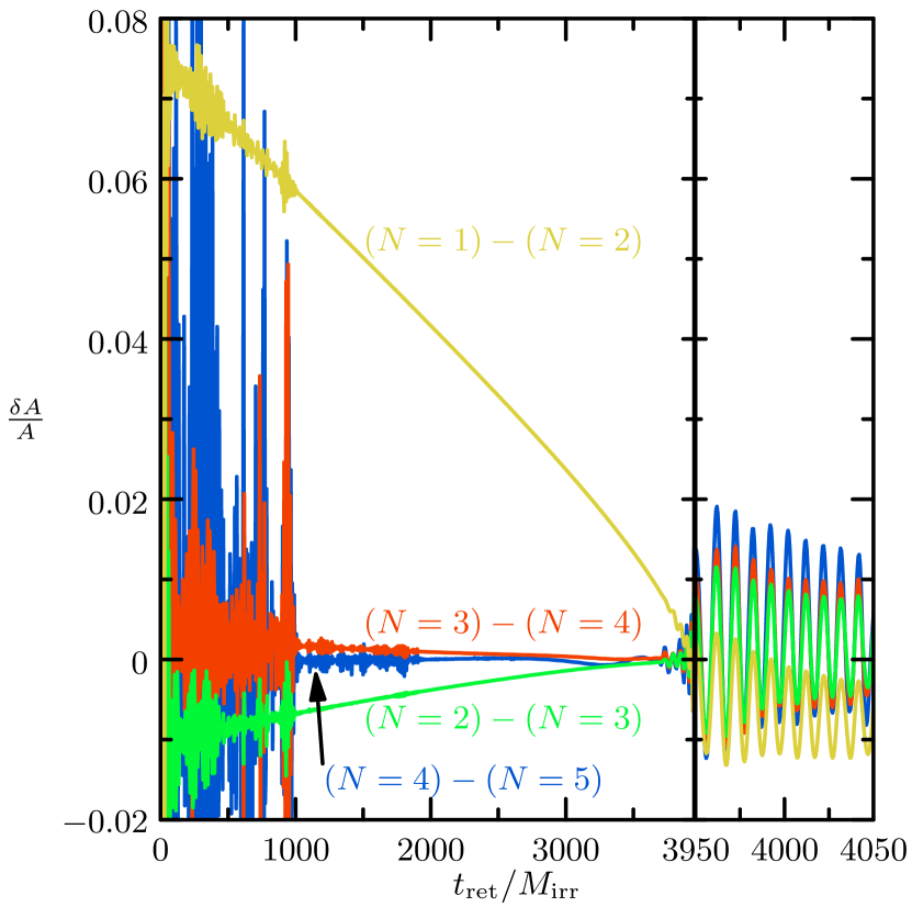
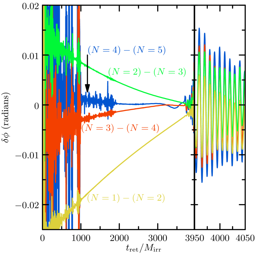
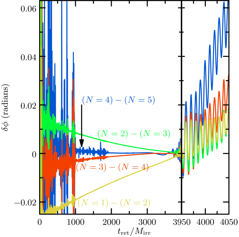
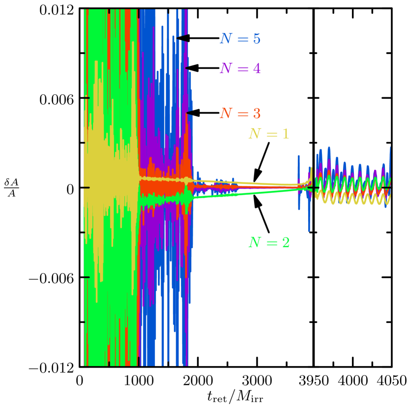
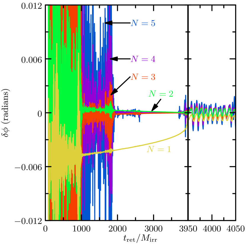
We show the results of these extrapolations in the figures below. Figs. 3 through 5 show convergence plots for extrapolations using orders –. The first two figures show the relative amplitude and phase difference between successive orders of extrapolation, using the corrected time of Eq. (14). Here, we define
| (17a) | |||
| and | |||
| (17b) | |||
When comparing waveforms extrapolated by polynomials of different orders, we use . Note that the broad trend is toward convergence, though high-frequency noise is more evident as the order increases, as we discuss further in the next subsection. The peak amplitude of the waves occurs at time . Note that the scale of the horizontal axis changes just before this time to better show the merger/ringdown portion. We see that the extrapolation is no longer convergent, with differences increasing slightly as the order of the extrapolating polynomial is increased. The oscillations we see in these convergence plots have a frequency equal to the frequency of the waves themselves. Their origin is not clear, but may be due to numerics, gauge, or other effects that violate our assumptions about the outgoing-wave nature of the data. It is also possible that there are simply no higher-order effects to be extrapolated, so low-order extrapolation suffices.
Figure 5 shows the same data as in Fig. 4, except that no correction is used for dynamic lapse. That is, for this figure (and only this figure), we use , where is simply the coordinate time. This demonstrates the need for improved time-retardation methods after merger. Note that the extrapolated data during the long inspiral is virtually unchanged (note the different vertical axes). After the merger—occurring at roughly —there is no convergence when no correction is made for dynamic lapse. It is precisely the merger and ringdown segment during which extreme gauge changes are present in the data used here Scheel et al. (2009). On the other hand, the fair convergence of the corrected waveforms indicates that it is possible to successfully remove these gauge effects.
II.4 Choosing the order of extrapolation
Deciding on an appropriate order of extrapolation to be used for a given purpose requires balancing competing effects. As we see in Fig. 3, for example, there is evidently some benefit to be gained from using higher-order extrapolation during the inspiral; there is clearly some convergence during inspiral for each of the orders shown. On the other hand, higher-order methods amplify the apparent noise in the waveform.101010So-called “junk radiation” is a ubiquitous feature of initial data for current numerical simulations of binary black-hole systems. It is clearly evident in simulations as large-amplitude, high-frequency waves that die out as the simulation progresses. While it is astrophysically extraneous, it is nevertheless a correct result of evolution from the initial data. Better initial data would, presumably, decrease its magnitude. This is the source of what looks like noise in the waveforms at early times. It is less apparent in data than in data because effectively amplifies high-frequency components, because of the relation . Moreover, late in the inspiral, and on into the merger and ringdown, the effects being extrapolated may be present only at low orders; increasing the extrapolation order would be useless as higher-order terms would simply be fitting to noise.
The optimal order depends on the accuracy needed, and on the size of effects that need to be eliminated from the data. For some applications, little accuracy is needed, so a low-order extrapolation (or even no extrapolation) is preferable.111111 We note that—as expected from investigations of near-field effects Teukolsky (1982); Boyle (2008, 2010)—the second-order behavior of the amplitude greatly dominates its first-order behavior Hannam et al. (2008). Thus, there is no improvement to the accuracy of the amplitude when extrapolating with ; it would be better to simply use the data from the largest extraction radius. If high-frequency noise is not considered a problem, then simple high-order extrapolation should suffice. Of course, if both high accuracy and low noise are required, data may easily be filtered, mitigating the problem of noise amplification. (See the appendix for more discussion.) There is some concern that this may introduce subtle inaccuracies: filtering is more art than science, and it is difficult to establish precise error bars for filtered data.
II.5 Choosing extraction radii
Another decision needs to be made regarding the number and location of extraction surfaces. Choosing the number of surfaces is fairly easy, because there is typically little cost in increasing the number of extraction radii (especially relative to the cost of—say—running a simulation). The only restriction is that the number of data points needs to be significantly larger than the order of the extrapolating polynomial; more can hardly hurt. More careful consideration needs to be given to the location of the extraction surfaces.
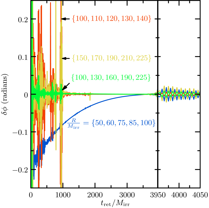
For the extrapolations shown in Figs. 3 and 4, data was extracted on spheres spaced by to , from to . The outer radius of was chosen simply because this is the largest radius at which data exists throughout the simulation; presumably, we always want the outermost radii at which the data are resolved. In choosing the inner radius, there are two competing considerations.
On one hand, we want the largest spread possible between the inner and outer extraction radii to stabilize the extrapolation. A very rough rule of thumb seems to be that the distance to be extrapolated should be no greater than the distance covered by the data. Because the extrapolating polynomial is a function of , the distance to be extrapolated is . The distance covered by the data is , so if the rule of thumb is to be satisfied, the inner extraction radius should be no more than half of the outer extraction radius, (noting, of course, that this is a very rough rule of thumb).
On the other hand, we would like the inner extraction radius to be as far out as possible. Extracting data near the violent center of the simulation is a bad idea for many reasons. Coordinate ambiguity, tetrad errors, near-field effects—all are more severe near the center of the simulation. The larger these errors are, the more work the extrapolation needs to do. This effectively means that higher-order extrapolation is needed if data are extracted at small radii. The exact inner radius needed for extrapolation depends on the desired accuracy and, again, the portion of the simulation from which the waveform is needed.
We can compare data extrapolated using different sets of radii. Figure 6 shows a variety, compared to the data used elsewhere in this paper. The extrapolation order is in all cases. Note that the waveforms labeled and both satisfy the rule of thumb that the inner radius should be at most half of the outer radius, while the other two waveforms do not; it appears that violation of the rule of thumb leads to greater sensitivity to noise. One waveform is extrapolated using only data from small radii, . It is clearly not converged, and would require higher-order extrapolation if greater accuracy is needed. The source of the difference is presumably the near-field effect Boyle (2008), which is proportionally larger at small radii.
Clearly, there is a nontrivial interplay between the radii used for extraction and the order of extrapolation. Indeed, because of the time-dependence of the various elements of these choices, it may be advisable to use different radii and orders of extrapolation for different time portions of the waveform. The different portions could then be joined together using any of various methods Ajith et al. (2008); Boyle et al. (2009).
III Extrapolation using the phase of the waveform
While the tortoise-coordinate method just described attempts to compensate for nontrivial gauge perturbations, it is possible that it does not take account of all effects adequately. As an independent check, we discuss what is essentially a second—very different—formulation of the retarded-time parameter, similar to one first introduced in Ref. Hannam et al. (2008). If waves extrapolated with the two different methods agree, then we can be reasonably confident that unmodeled gauge effects are not diminishing the accuracy of the final result. As we will explain below, the method in this section cannot be used naively with general data (e.g., data on the equatorial plane). In particular, we must assume that the data to be extrapolated consists of a strictly monotonic phase. It is, however, frequently possible to employ a simple technique to make purely real, oscillating data into complex data with strictly monotonic phase, as we describe below. The results of this technique agree with those of the tortoise-coordinate extrapolation as we show in Sec. IV.
Instead of extrapolating the wave phase and amplitude as functions of time and radius, we extrapolate the time and the amplitude as functions of wave phase and radius . In other words, we measure the amplitude and the arrival time to some radius of a fixed phase point in the waveform. This is the origin of the requirement that the data to be extrapolated consist of a strictly monotonic phase (i.e., it must be invertible). For the data presented here, the presence of radiation in the initial data—junk radiation—and numerical noise cause the extracted waveforms to fail to satisfy this requirement at early times. In this case, the extrapolation is performed separately for each invertible portion of the data. That is, the data are divided into invertible segments, each segment is extrapolated separately, and the final products are joined together as a single waveform.
III.1 Description of the method
This extrapolation technique consists of extrapolating the retarded time and the amplitude as functions of the wave phase and the radius . In other words, when extrapolating the waveform, we are estimating the amplitude and the arrival time of a fixed phase point at infinity. Here, we extract the same , , and areal-radius data used in the previous section. As in the previous method, we first shift each waveform in time using , where is defined in Eq. (14) and the basic tortoise coordinate is defined in Eq. (7) with areal radius as the radial parameter. The amplitude and wave phase are again defined using Eq. (15), and the phase is made continuous as in Sec. II.3. Thus, we begin with the same data, shifted as with the tortoise-coordinate method.
Now, however, we change the method, in an attempt to allow for unmodeled effects. Instead of extrapolating and , as with the previous method, we invert these functions to get and as functions of the wave phase . In other words, we extrapolate the arrival time and the amplitude of a signal to a coordinate radius for each wave phase value. This is done by fitting the retarded time and the amplitude data to polynomials in for each value of the wave phase:
| (18a) | ||||
| (18b) | ||||
where the asymptotic waveform is fully described by and .
With this data in hand, we can produce the asymptotic amplitude and phase as functions of time by plotting curves in the – and – planes parametrized by the phase. In order to be true, single-valued functions, we again need monotonicity of the data, which may be violated by extrapolation. The usable data can be obtained simply by removing data from times before which this condition holds.
Choosing the extraction radii and extrapolation order for this method follows the same rough recommendations described in Secs. II.4 and II.5. Note also that the restriction that the data have an invertible phase as a function of time is not insurmountable. For example, data for in the equatorial plane is purely real, hence has a phase that simply jumps from to discontinuously. However, we can define a new quantity
| (19) |
This is simply an auxiliary quantity used for the extrapolation, with a smoothly varying, invertible phase. The imaginary part is discarded after extrapolation.
III.2 Results
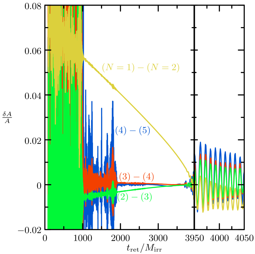
In Figs. 7 and 8 we plot the convergence of the relative amplitude and phase of the extrapolated mode of the waveform for extrapolation orders . A common feature of both plots is that during the inspiral, the higher the extrapolation order, the better the convergence. However, the noise is amplified significantly for large orders of extrapolation. This method of extrapolation amplifies high-frequency noise significantly, compared to the tortoise-coordinate method.
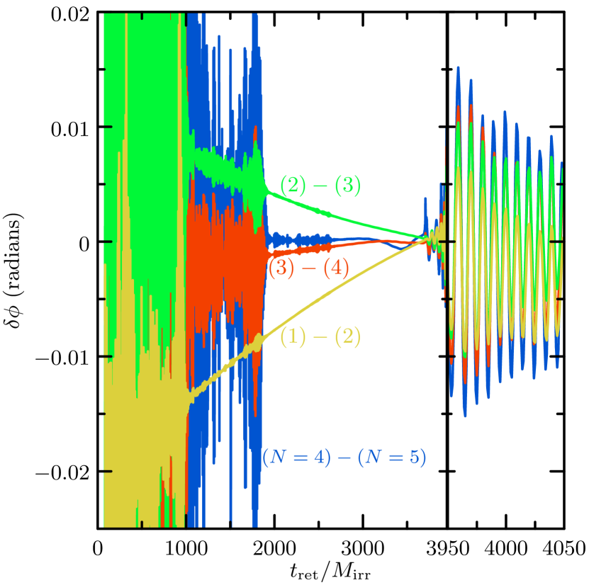
In the inspiral portion, we have a decreasing error in the extrapolation of the phase and the amplitude as the wavelength of the gravitational waves decreases. In the merger/ringdown portion, a more careful choice of the radii and order of extrapolation needs to be made. Since near-field effects are less significant in the data extracted at larger radii, extrapolation at low order () seems sufficient. Data extrapolated at large order () has a larger error in the phase and amplitude after merger than data extrapolated at order or . Moreover, the outermost extraction radius could be reduced, say to instead of , without having large extrapolation error at late times. Using the radius range instead of the range would leave the extrapolation error during the merger/ringdown almost unchanged, while the extrapolation error during the inspiral would increase by about 70%.
We note that this method allows easy extrapolation of various portions of the waveform using different extraction radii and orders since—by construction—the wave phase is an independent variable. For example, solve for the phase value of the merger (defined as the phase at which the amplitude is a maximum), then use the radius range for all phase values less than and the range for all larger phase values.
This method has been tested also using the coordinate radius and the naive time coordinate , in place of areal radius and corrected time. We found results similar to those discussed in Sec. II. Using the new time coordinate instead of the naive time coordinate improved the extrapolation during the merger/ringdown, as found in Sec. II.
As with the previous extrapolation method, increasing the extrapolation order gives a faster convergence rate of waveform phase and amplitude, but it amplifies noise in the extrapolated waveform. To improve convergence without increasing the noise, we need a good filtering technique for the inspiral data. The junk-radiation noise decreases significantly as a function of time, disappearing several orbits before merger. However, this noise could be reduced by using more extraction radii in the extrapolation process, or by running the data through a low-pass filter. See the appendix for further discussion of filtering.
IV Comparison of the two methods
Both methods showed good convergence of the amplitude and the phase of the waveform as increased in the inspiral portion. (See Figs. 3 and 7 for the amplitude, and Figs. 4 and 8 for the phase.) The wave-phase extrapolation method was more sensitive to noise. In the merger/ringdown portion, both methods have similar convergence as increases, especially when the correction is taken to account for the dynamic lapse. The use of the time parameter improved the agreement between the methods significantly in the merger/ringdown portion for all extrapolation orders. Extrapolating at order or seems the best choice as the noise and phase differences are smallest for these values.
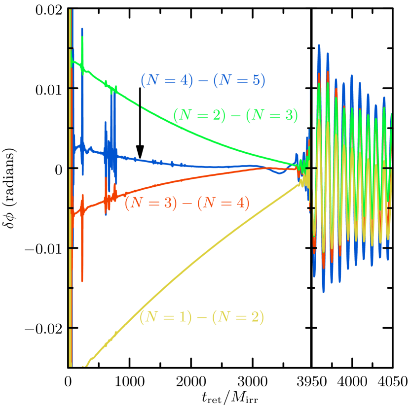
In Fig. 9, we show the relative amplitude difference between data extrapolated at various orders (). There is no additional time or phase offset used in the comparison. Ignoring high-frequency components, the difference in the relative amplitude is always less than 0.3% for different extrapolation orders. Even including high-frequency components, the differences between the two methods are always smaller than the error in each method, as judged by convergence plots. In Fig. 10, we show the phase difference between the data extrapolated using both methods. As in the relative amplitude-difference plots, the best agreement is achieved during the inspiral portion. Ignoring high-frequency components, the difference is less than 0.02 radians for all orders. In the merger/ringdown portion, the best agreement between extrapolated waveforms is at order or where the phase difference is less than 0.01 radians.
V Conclusions
We have demonstrated two simple techniques for extrapolating gravitational-wave data from numerical-relativity simulations. We took certain basic gauge information into account to improve convergence of the extrapolation during times of particularly dynamic gauge, and showed that the two methods agree to within rough error estimates. We have determined that the first method presented here is less sensitive to noise, and more immediately applies to arbitrary wavelike data; this method has become the basic standard in use by the Caltech–Cornell collaboration. In both cases, there were problems with convergence after merger. The source of these problems is still unclear, but will be a topic for further investigation.
As with any type of extrapolation, a note of caution is in order. It is entirely possible that the “true” function being extrapolated bears little resemblance to the approximating function we choose, outside of the domain on which we have data. We may, however, have reason to believe that the true function takes a certain form. If the data in question are generated by a homogeneous wave equation, for instance, we know that well-behaved solutions fall off in powers of . In any case, there is a certain element of faith that extrapolation is a reasonable thing to do. While that faith may be misplaced, there are methods of checking whether or not it is: goodness-of-fit statistics, error estimates, and convergence tests. To be of greatest use, goodness-of-fit statistics and error estimates for the output waveform require error estimates for the input waveforms. We leave this for future work.
We still do not know the correct answers to the questions numerical relativity considers. We have no analytic solutions to deliver the waveform that Einstein’s equations—solved perfectly—predict would come from a black-hole binary merger; or the precise amount of energy radiated from any given binary; or the exact kick or spin of the final black hole. Without being able to compare numerical relativity to exact solutions, we may be leaving large systematic errors hidden in plain view. To eliminate them, we need to use multiple, independent methods for our calculations. For example, we might extract directly by calculating the Riemann tensor and contracting appropriately with our naive coordinate tetrad, and extract the metric perturbation using the formalism of Regge–Wheeler–Zerilli and Moncrief. By differentiating the latter result twice and comparing to , we could verify that details of the extraction methods are not producing systematic errors. (Just such a comparison was done in Ref. Buonanno et al. (2009) for waveforms extrapolated using the technique in this paper.) Nonetheless, it is possible that infrastructure used to find both could be leading to errors.
In the same way, simulations need to be performed using different gauge conditions, numerical techniques, code infrastructures, boundary conditions, and even different extrapolation methods. Only when multiple schemes arrive at the same result can we be truly confident in any of them. But to arrive at the same result, the waveforms from each scheme need to be processed as carefully as possible. We have shown that extrapolation is crucial for highly accurate gravitational waveforms, and for optimized detection of mergers in detector data.
Acknowledgements.
We thank Emanuele Berti, Duncan Brown, Luisa Buchman, Alessandra Buonanno, Yanbei Chen, Éanna Flanagan, Mark Hannam, Sascha Husa, Luis Lehner, Geoffrey Lovelace, Andrea Nerozzi, Rob Owen, Larne Pekowsky, Harald Pfeiffer, Oliver Rinne, Uli Sperhake, Béla Szilágyi, Kip Thorne, Manuel Tiglio, and Alan Weinstein for helpful discussions. We especially thank Larry Kidder, Lee Lindblom, Mark Scheel, and Saul Teukolsky for careful readings of this paper in various draft forms and helpful comments. This research has been supported in part by a grant from the Sherman Fairchild Foundation to Caltech and Cornell; by NSF Grants PHY-0652952, PHY-0652929 and DMS-0553677 and NASA Grant NNX09AF96G to Cornell; and by NSF grants PHY-0601459, PHY-0652995, DMS-0553302 and NASA grant NNG05GG52G to Caltech.*
Appendix A Filtering
Extrapolating waveforms containing poorly resolved high-frequency components amplifies the magnitude of the noise in the signal at infinity. One possible solution to the problem is to filter out the junk radiation from the gravitational waveform. This is possible when the noise has higher frequency than the physical data of interest. The Matlab function filtfilt, using a low-pass Butterworth filter with cutoff frequency between the noise frequency and the highest gravitational-wave frequency, is satisfactory for many uses when applied to the early parts of the data. This filtering may be applied to either the complex data, or to its amplitude and phase—the latter allowing for a lower cutoff frequency. There is also a marginal benefit to be gained when the input data are filtered before extrapolation, though filtering of the final result is also necessary. It is also possible to fit a low-order polynomial to the data, filter the residual, and add the filtered data back to the fit; this removes very low-frequency components, reducing the impact of Gibbs phenomena.
For the data presented here, we use a sixth-order Butterworth filter with a physical cutoff frequency of ,121212Note that Matlab expects the input frequency as a fraction of the data’s Nyquist frequency. which is roughly eight times the maximum frequency of the physical waveforms expected in the filtered region. The filter is applied individually (using the filtfilt function) to the amplitude and phase data, in turn. Because of remaining Gibbs phenomena at late times, we use unfiltered data after .
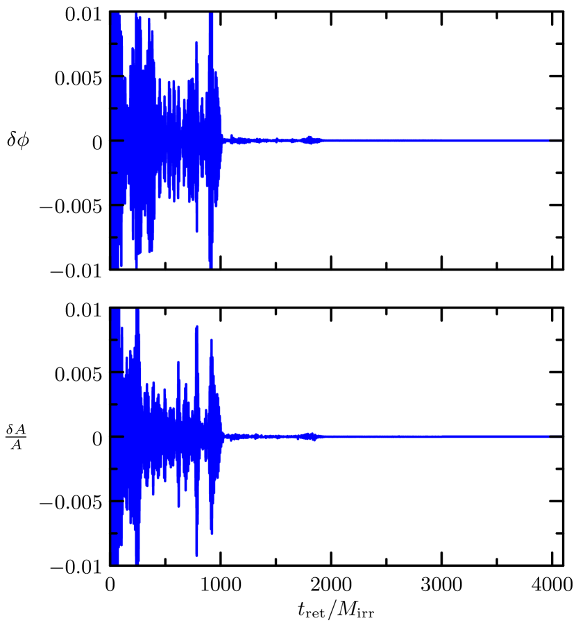
One basic diagnostic of the filtering process is to simply look at the difference between filtered and unfiltered data. If there are low-frequency components in these curves, we know the cutoff frequency needs to be raised. In Fig. 11, we show the difference in relative amplitude (upper panel), and phase (lower panel). Because there is no difference between the filtered and unfiltered waveforms on the timescale of the physical gravitational waves (), we conclude that the filter’s cutoff frequency is high enough to retain the physical information.
On the other hand, to check that the filter’s cutoff frequency is low enough to achieve its purpose, we look at data which previously showed the undesirable high-frequency characteristics. In Fig. 12, we show the same data as in Fig. 4, when the data are filtered before subtraction. The size of the noise at early times is greatly reduced. There are still significant high-frequency features in the plot, though they are much smaller than in the unfiltered data. Presumably these features are simply so large in the input data that even with the large suppression from the filter, they are still noticeable. It may be possible to remove them by further decreasing the filter’s cutoff frequency, though this would require better handling of Gibb’s phenomena from the beginning and end of the wave. We find the present filter sufficient for the demonstration purposes of this appendix.
References
- Teukolsky (1982) S. A. Teukolsky, Phys. Rev. D 26, 745 (1982), URL http://link.aps.org/abstract/PRD/v26/p745.
- Boyle (2008) M. Boyle, Ph.D. thesis, California Institute of Technology (2008), URL http://etd.caltech.edu/etd/available/etd-01122009-143851/unre%%****␣paper.bbl␣Line␣25␣****stricted/Thesis.pdf.
- Boyle (2010) M. Boyle (2010), in preparation.
- Hannam et al. (2008) M. Hannam, S. Husa, J. A. González, U. Sperhake, and B. Brügmann, Phys. Rev. D 77, 044020 (pages 15) (2008), URL http://link.aps.org/abstract/PRD/v77/e044020.
- Finn (1992) L. S. Finn, Phys. Rev. D 46, 5236 (1992), URL http://link.aps.org/abstract/PRD/v46/p5236.
- Finn and Chernoff (1993) L. S. Finn and D. F. Chernoff, Phys. Rev. D 47, 2198 (1993), URL http://link.aps.org/abstract/PRD/v47/p2198.
- Boyle et al. (2009) M. Boyle, D. A. Brown, and L. Pekowsky, Class. Quant. Grav. 26, 114006 (2009), URL http://stacks.iop.org/0264-9381/26/114006.
- Hannam et al. (2009) M. Hannam, S. Husa, J. G. Baker, M. Boyle, B. Brugmann, T. Chu, N. Dorband, F. Herrmann, I. Hinder, B. J. Kelly, et al., Phys. Rev. D 79, 084025 (2009), URL http://link.aps.org/abstract/PRD/v79/e084025.
- Brown (2004) D. A. Brown, Ph.D. thesis, University of Wisconsin–Milwaukee (2004), URL http://arxiv.org/abs/0705.1514.
- Lindblom et al. (2008) L. Lindblom, B. J. Owen, and D. A. Brown, Phys. Rev. D 18, 124020 (pages 12) (2008), URL http://link.aps.org/abstract/PRD/v78/e124020.
- Buonanno et al. (2007) A. Buonanno, G. B. Cook, and F. Pretorius, Phys. Rev. D 75, 124018 (pages 42) (2007), URL http://link.aps.org/abstract/PRD/v75/e124018.
- Campanelli et al. (2006) M. Campanelli, C. O. Lousto, P. Marronetti, and Y. Zlochower, Phys. Rev. Lett. 96, 111101 (pages 4) (2006), URL http://link.aps.org/abstract/PRL/v96/e111101.
- Baker et al. (2006) J. G. Baker, J. Centrella, D.-I. Choi, M. Koppitz, and J. van Meter, Phys. Rev. Lett. 96, 111102 (pages 4) (2006), URL http://link.aps.org/abstract/PRL/v96/e111102.
- Nerozzi et al. (2005) A. Nerozzi, C. Beetle, M. Bruni, L. M. Burko, and D. Pollney, Phys. Rev. D 72, 024014 (pages 13) (2005), URL http://link.aps.org/abstract/PRD/v72/e024014.
- Sarbach and Tiglio (2001) O. Sarbach and M. Tiglio, Phys. Rev. D 64, 084016 (2001), URL http://link.aps.org/abstract/PRD/v64/e084016.
- Pazos et al. (2007) E. Pazos, E. N. Dorband, A. Nagar, C. Palenzuela, E. Schnetter, and M. Tiglio, Class. Quant. Grav. 24, S341 (2007), URL http://stacks.iop.org/0264-9381/24/S341.
- Thorne (1980) K. S. Thorne, Rev. Mod. Phys. 52, 299 (1980), URL http://link.aps.org/abstract/RMP/v52/p299.
- Abrahams and Evans (1988) A. M. Abrahams and C. R. Evans, Phys. Rev. D 37, 318 (1988), URL http://link.aps.org/abstract/PRD/v37/p318.
- Abrahams and Evans (1990) A. M. Abrahams and C. R. Evans, Phys. Rev. D 42, 2585 (1990), URL http://link.aps.org/abstract/PRD/v42/p2585.
- Deadman and Stewart (2009) E. Deadman and J. M. Stewart, Class. Quant. Grav. 26, 065008 (2009), URL http://stacks.iop.org/0264-9381/26/065008.
- Bishop et al. (1996) N. T. Bishop, R. Gómez, L. Lehner, and J. Winicour, Phys. Rev. D 54, 6153 (1996), URL http://link.aps.org/abstract/PRD/v54/p6153.
- Hübner (2001) P. Hübner, Class. Quant. Grav. 18, 1871 (2001), URL http://stacks.iop.org/0264-9381/18/1871.
- Babiuc et al. (2005) M. Babiuc, B. Szilágyi, I. Hawke, and Y. Zlochower, Class. Quant. Grav. 22, 5089 (2005), URL http://stacks.iop.org/0264-9381/22/5089.
- Babiuc et al. (2009) M. C. Babiuc, N. T. Bishop, B. Szilágyi, and J. Winicour, Phys. Rev. D 79, 084011 (pages 18) (2009), URL http://link.aps.org/abstract/PRD/v79/e084011.
- Boyle et al. (2007) M. Boyle, D. A. Brown, L. E. Kidder, A. H. Mroué, H. P. Pfeiffer, M. A. Scheel, G. B. Cook, and S. A. Teukolsky, Phys. Rev. D 76, 124038 (pages 31) (2007), URL http://link.aps.org/abstract/PRD/v76/e124038.
- Boyle et al. (2008) M. Boyle, A. Buonanno, L. E. Kidder, A. H. Mroué, Y. Pan, H. P. Pfeiffer, and M. A. Scheel, Phys. Rev. D 78, 104020 (pages 23) (2008), URL http://link.aps.org/abstract/PRD/v78/e104020.
- Scheel et al. (2009) M. A. Scheel, M. Boyle, T. Chu, L. E. Kidder, K. D. Matthews, and H. P. Pfeiffer, Phys. Rev. D 79, 024003 (pages 14) (2009), URL http://link.aps.org/abstract/PRD/v79/e024003.
- Buonanno et al. (2009) A. Buonanno, Y. Pan, H. P. Pfeiffer, M. A. Scheel, L. T. Buchman, and L. E. Kidder, Phys. Rev. D 79, 124028 (pages 19) (2009), URL http://link.aps.org/abstract/PRD/v79/e124028.
- Press et al. (2007) W. H. Press, S. A. Teukolsky, W. T. Vetterling, and B. P. Flannery, Numerical Recipes: The Art of Scientific Computing (Cambridge University Press, 2007), 3rd ed., ISBN 0-52-188068-8.
- Damour et al. (2008) T. Damour, A. Nagar, M. Hannam, S. Husa, and B. Brügmann, Phys. Rev. D 78, 044039 (pages 24) (2008), URL http://link.aps.org/abstract/PRD/v78/e044039.
- Chandrasekhar (1992) S. Chandrasekhar, The Mathematical Theory of Black Holes (Oxford University Press, 1992), ISBN 0-19-852050-6.
- Kocsis and Loeb (2007) B. Kocsis and A. Loeb, Phys. Rev. D 76, 084022 (pages 14) (2007), URL http://link.aps.org/abstract/PRD/v76/e084022.
- Ajith et al. (2008) P. Ajith, S. Babak, Y. Chen, M. Hewitson, B. Krishnan, A. M. Sintes, J. T. Whelan, B. Brügmann, P. Diener, N. Dorband, et al., Phys. Rev. D 77, 104017 (pages 22) (2008), URL http://link.aps.org/abstract/PRD/v77/e104017.