THC: a new high-order finite-difference high-resolution shock-capturing code for special-relativistic hydrodynamics

We present THC: a new high-order flux-vector-splitting code for Newtonian and special-relativistic hydrodynamics designed for direct numerical simulations of turbulent flows. Our code implements a variety of different reconstruction algorithms, such as the popular weighted essentially non oscillatory and monotonicity-preserving schemes, or the more specialised bandwidth-optimised WENO scheme that has been specifically designed for the study of compressible turbulence.

We show the first systematic comparison of these schemes in Newtonian physics as well as for special-relativistic flows. In particular we will present the results obtained in simulations of grid-aligned and oblique shock waves and nonlinear, large-amplitude, smooth adiabatic waves. We will also discuss the results obtained in classical benchmarks such as the double-Mach shock reflection test in Newtonian physics or the linear and nonlinear development of the relativistic Kelvin-Helmholtz instability in two and three dimensions. Finally, we study the turbulent flow induced by the Kelvin-Helmholtz instability and we show that our code is able to obtain well-converged velocity spectra, from which we benchmark the effective resolution of the different schemes.

1 Introduction

Numerical relativistic hydrodynamics has come a long way since the pioneering works by May & White (1966) and Wilson (1972) and it is now playing a central role in modelling of systems involving strong gravity and/or flows with high Lorentz factors. Example of applications are relativistic jets, core-collapse supernovae, merger of compact binaries and the study of gamma-ray bursts [see Martí & Müller (2003) and Font (2008) for a complete overview].

In all of these areas the progress has been continuous over the past few years to the point that relativistic computational fluid dynamics is starting to provide a realistic description of many relativistic-astrophysics scenarios [see, e.g. Rezzolla et al. (2011)]. Key factors in this progress have been the switch to more advanced and accurate numerical schemes, and in particular the adoption of high resolution shock capturing (HRSC) schemes (Martí et al. 1991; Schneider et al. 1993; Banyuls et al. 1997; Donat et al. 1998; Aloy et al. 1999; Baiotti et al. 2003) and the progressive inclusion of more “physics” for a more accurate description of the different scenarios. Examples of the latter are the inclusion of magnetic fields (Koide et al. 1999; Del Zanna et al. 2003; Gammie et al. 2003; Komissarov 2004; Duez et al. 2005; Neilsen et al. 2006; Antón et al. 2006; Giacomazzo & Rezzolla 2007) the use of realistic tabulated equations of state, [see, e.g. Sekiguchi et al. (2011)], and the description of radiative processes (Farris et al. 2008; Sekiguchi 2010; Zanotti et al. 2011).

We expect that both improved physical models and better numerical techniques will be key elements in the future generation of codes for relativistic astrophysics. On the one hand it is necessary to take into account many physical phenomena that are currently oversimplified and, on the other hand, higher accuracy is necessary to make quantitative predictions even in the case where simplified models are used to describe the objects of study. For example, in the case of inspiralling binary neutron stars, waveforms that are sufficiently accurate for gravitational-waves templates are just now becoming available and only in the simple case of polytropic stars (Baiotti et al. 2009, 2010; Bernuzzi et al. 2012b). Clearly, even higher accuracy will be required as more realistic equations of state are considered or better characterisations of the tidal effects are explored (Baiotti et al. 2011; Bernuzzi et al. 2012a).

For this reason the development of more accurate numerical tools for relativistic hydrodynamics is an active and lively field of research. Most of the effort has been directed towards the development of high-order finite-volume (Tchekhovskoy et al. 2007; Duffell & MacFadyen 2011) and finite-difference (Zhang & MacFadyen 2006; Del Zanna et al. 2007) schemes, but many alternative approaches have been also proposed, including finite-element methods (Mann 1985; Meier 1999), spectral methods (Gourgoulhon 1991), smoothed-particle-hydrodynamics (Siegler & Riffert 2000; Rosswog 2010) and discontinuous Galerkin methods (Dumbser & Zanotti 2009; Radice & Rezzolla 2011).

The use of flux-conservative finite-difference HRSC schemes is probably the easiest way of increasing the (formal) order of accuracy of the current generation of numerical codes: finite-difference schemes are much cheaper then high-order finite-volume codes since they do not require the solution of multiple Riemann problems at the interface between different regions (Shu 1999, 2001) and they are free from the complicated averaging and de-averaging procedures of high-order finite-volume codes [see, e.g. Tchekhovskoy et al. (2007)].

Here we present a new code, the Templated-Hydrodynamics Code (THC), developed using the Cactus framework (Goodale et al. 2003), that follows this approach. THC employs a state-of-the-art flux-vector splitting scheme: it uses up to seventh-order reconstruction in characteristics fields and the Roe flux split with a novel entropy-fix prescription. The “templated” aspect reflects the fact that the code design is based on a modern C$++$ paradigm called template metaprogramming, in which part of the code is generated at compile time. Using this particular programming technique it is possible to construct object-oriented, highly modular, codes without the extra computational costs associated with classical polymorphism, because, in the templated case, polymorphism is resolved at compile time allowing the compiler to inline all the relevant function calls, see e.g. Yang (2000). Among the different reconstruction schemes that we implemented are the classical monotonicity-preserving (MP) MP5 scheme (Suresh & Huynh 1997; Mignone et al. 2010), the weighted essentially non oscillatory (WENO) schemes WENO5 and WENO7 (Liu et al. 1994; Jiang & Shu 1996; Shu 1997) and two bandwidth-optimized WENO schemes: WENO3B and WENO4B (Martín et al. 2006; Taylor et al. 2007), designed for direct simulations of compressible turbulence (we recall that the number associated to the different methods indicates the putative order of accuracy).

By far the largest motivation behind the development of THC is the study of the statistical properties of relativistic turbulence and the determination of possible new and non-classical features. In a recent paper (Radice & Rezzolla, in prep.), we have presented the results of direct numerical simulations of driven turbulence in an ultrarelativistic hot plasma obtained using THC. More specifically, we have studied the statistical properties of flows with average Mach number ranging from $\sim 0.4$ to $\sim 1.7$ and with average Lorentz factors up to $\sim 1.7$, finding that flow quantities, such as the energy density or the local Lorentz factor, show large spatial variance even in the subsonic case as compressibility is enhanced by relativistic effects. We have also uncovered that the velocity field is highly intermittent, but its power-spectrum is found to be in good agreement with the predictions of the classical theory of Kolmogorov. Overall, the results presented in Radice & Rezzolla in prep. indicate that relativistic effects are able to enhance significantly the intermittency of the flow and affect the high-order statistics of the velocity field, while leaving unchanged the low-order statistics, which appear to be universal and in good agreement with the classical Kolmogorov theory.

In this paper we give the details of the algorithms used in THC and employed in Radice & Rezzolla in prep., presenting a systematic comparison between the results obtained using the above mentioned reconstruction schemes, with emphasis for the application of these schemes for direct simulations of relativistic turbulence. To our knowledge this is the first time that such a comparison has been done in the relativistic case.

The rest of this paper is organised as follows. In Section 2 we present THC code in more detail: we discuss the numerical algorithms it uses and recall the equations of Newtonian and special-relativistic hydrodynamics. The results obtained with our code in a representative number of test cases for the Newtonian and special relativistic hydrodynamics are presented in Section 3. In Section 4 we present the application of our code to the study of the linear and nonlinear development of the relativistic Kelvin-Helmholtz instability (KHI) in three dimensions as a nontrivial application for our code and a stringent test of its accuracy. Finally Section 5 is dedicated to the summary and the conclusions.

2 The Templated-Hydrodynamics Code

We here briefly outline the numerical infrastructure adopted by our templated-hydrodynamics code and report the formulations of the equations of Newtonian and special-relativistic hydrodynamics we actually solve.

2.1 Finite-differencing high-resolution shock-capturing schemes

We can only provide here a minimal description of the numerical schemes used by THC and we refer the interested reader to Shu (1999) for a more detailed description of finite-difference ENO/WENO HRSC schemes, and to Mignone et al. (2010) for a detailed description of the finite-difference MP5 scheme. We also note that an approach very similar to ours was already adopted by Zhang & MacFadyen (2006) in the construction of the RAM code.

Both in the case of the Newtonian and in that of the relativistic-hydrodynamic equations, we consider a system of hyperbolic balance-laws in the form

$$\frac{\partial\boldsymbol{F}^{0}(\boldsymbol{u})}{\partial t}+\sum_{i=1}^{3}\frac{\partial\boldsymbol{F}^{i}(\boldsymbol{u})}{\partial x^{i}}=\boldsymbol{S}(\boldsymbol{u})\,,$$ (1)

where the components of $\boldsymbol{u}$ are the so-called primitive variables, a set of $N$ independent physical quantities, $N$ being the number of equations composing (1), while $\boldsymbol{F}^{0}(\boldsymbol{u})$ is referred to as the vector of conserved variables (or state vector), even though they are not strictly conserved in the presence of a source term $\boldsymbol{S}(\boldsymbol{u})$.

As customary with grid-based codes, we solve numerically the set of equations (1) on a computational grid defined in a Cartesian coordinate system at uniformly distributed spatial positions

$$\boldsymbol{x}_{i,j,k}=(i\Delta^{1},j\Delta^{2},k\Delta^{3})\,,\qquad i,j,k\in\mathbb{Z}\,,$$ (2)

and rewrite it using the method of lines, in a semi-discrete, dimensionally unsplit form as

$$\frac{d\boldsymbol{F}^{0}_{i,j,k}}{dt}=\boldsymbol{S}_{i,j,k} +\frac{\boldsymbol{F}^{1}_{i-1/2,j,k}-\boldsymbol{F}^{1}_{i+1/2,j,k}}{\Delta^{1}}$$

$$+\frac{\boldsymbol{F}^{2}_{i,j-1/2,k}-\boldsymbol{F}^{2}_{i,j+1/2,k}}{\Delta^{2}}+\frac{\boldsymbol{F}^{3}_{i,j,k-1/2}-\boldsymbol{F}^{3}_{i,j,k+1/2}}{\Delta^{3}},$$ (3)

where $\psi_{i,j,k}$ is the value of a generic quantity, $\psi$, at $\boldsymbol{x}_{i,j,k}$, while $(\boldsymbol{F}^{1}_{i-1/2,j,k}-\boldsymbol{F}^{1}_{i+1/2,j,k})/\Delta^{1}$ is an high-order, non-oscillatory, approximation of $-\partial\boldsymbol{F}^{1}/\partial x^{1}$ at $\boldsymbol{x}_{i,j,k}$, to be specified. We use the method of lines to evolve (2.1) using a third-order strong stability-preserving Runge-Kutta (SSP-RK) scheme (Gottlieb et al. 2009).

To illustrate how we compute the discrete derivatives in the right-hand-side of (2.1) it is useful to make a step back and consider, first a simpler scalar hyperbolic equation in one dimension, i.e.

$$\frac{\partial u}{\partial t}+\frac{\partial f(u)}{\partial x}=0.$$ (4)

Introducing a uniform grid, $x_{i}=i\Delta$, and define, for any function, $v(x)$ the volume averages

$$\tilde{v}_{i}\equiv\frac{1}{\Delta}\int_{x_{i-1/2}}^{x_{i+1/2}}v(x)\,dx.$$ (5)

A reconstruction operator, $\mathcal{R}$, is a nonlinear operator yielding an high-order approximation of $v$ at a given point $x$ using its volume averages, $\tilde{v}_{i}$. Since $v(x)$ can be discontinuous, we distinguish two different reconstruction operators, $\mathcal{R}^{-}$ and $\mathcal{R}^{+}$, called the left-biased and right-biased reconstruction operators, such that

$$\left[\mathcal{R}^{-}\left(\{\tilde{v}_{i}\}\right)\right](x)=\lim_{y\to x^{-}}v(y)+\mathcal{O}(\Delta^{r})\,,$$ (6)

$$\left[\mathcal{R}^{+}\left(\{\tilde{v}_{i}\}\right)\right](x)=\lim_{y\to x^{+}}v(y)+\mathcal{O}(\Delta^{r})\,,$$ (7)

where we have indicated with $\mathcal{R}^{+}\left(\{\tilde{v}_{i}\}\right)$ the notion that $\mathcal{R}$ is an operator that acts on a set of averages $\tilde{v}_{i}$, and where $r$ is the order of the reconstruction operator $\mathcal{R}$. Hereafter we will use the notation $v_{i+1/2}^{-}$ and $v_{i+1/2}^{+}$ to denote the reconstructed values in $x_{i+1/2}$ using $\mathcal{R}^{-}$ and $\mathcal{R}^{+}$ respectively. Example of such operators are given by the ENO/WENO and the MP5 algorithms.

In classical WENO schemes, the reconstruction is obtained from a weighted average of a set of lower-order reconstructions of the $\tilde{v}_{i}$’s on a number of overlapping stencils. The weights are computed using some nonlinear smoothness indicators designed in such a way that the maximum possible order of accuracy is obtained in the case of smooth solutions. On the other hand, when discontinuities are detected, the order is automatically reduced to avoid spurious oscillations. The bandwidth-optimized WENO schemes differ from the classical ones because they use a more symmetric stencil and because their weights are not designed to yield the maximum possible formal order of accuracy for smooth solutions, but are instead tuned to minimise the attenuation of high-frequency modes. In other words, while in the classical WENO case the weights for a smooth function are chosen to match as many terms as possible in the Taylor expansion of the target function, in the bandwidth-optimized case the coefficients are chosen to yield the best possible approximation of the Fourier coefficients of the function to be reconstructed. The nonlinear smoothness indicators are also modified to avoid “over-adaptation” of the scheme and minimise the amount of numerical dissipation [see Martín et al. (2006); Taylor et al. (2007) for details].

The MP5 scheme, on the other hand, is based on a fifth-order reconstruction combined with a flattening procedure designed to avoid the creation of artificial extrema in the function to be reconstructed. The monotonicity-preserving reconstruction has the nice property that no spurious oscillations can be produced by the reconstruction, which is not guaranteed for the WENO schemes. On the other hand the limiting procedure employed by MP5 requires the use of a series of conditional statements in the code, that are not present in the WENO case.

The reconstruction operators are the core ingredients of both finite-volume and finite-difference schemes. In a finite-volume scheme they are used to compute the left and right state to be used in the (usually approximate) Riemann solver to compute the fluxes. In a finite-difference scheme, instead, they are used to compute the above mentioned non-oscillatory approximation of $\partial f/\partial x$. Following Shu & Osher (1988) we introduce a function $h(x)$ and such that

$$f\big{[}u(x_{i})\big{]}=\frac{1}{\Delta}\int_{x_{i-1/2}}^{x_{i+1/2}}h(\xi)\,d\xi\,,$$ (8)

that is, the average of $h(x)$ between $x_{i-1/2}$ and $x_{i+1/2}$ corresponds to the value of $f$ at $x_{i}$. Next, we note that

$$\frac{\partial f}{\partial x}\bigg{|}_{x_{i}}=\frac{h(x_{i+1/2})-h(x_{i-1/2})}{\Delta}\,,$$ (9)

where both (8) and (9) are exact expressions. Hence, by using the usual reconstruction operators $\mathcal{R}$ of order $r$ to reconstruct $h_{i+1/2}$, one obtains a corresponding accurate approximation of order $r$ of the derivative $\partial f/\partial x$ at $x_{i}$. Note that $h$ is never actually computed at any time during the calculation as we only need the values of $f$ at the gridpoints, i.e. $f\big{[}u(x_{i})\big{]}$.

In order to ensure the stability of the resulting scheme, one has to take care to upwind the reconstruction appropriately. Let us first consider the case in which $f^{\prime}(u)\equiv\partial f/\partial u>0$. If we set

$$\tilde{v}_{i}=f\big{[}u(x_{i})\big{]}=\frac{1}{\Delta}\int_{x_{i-1/2}}^{x_{i+1/2}}h(\xi)\,d\xi$$ (10)

and

$$f_{i+1/2}\equiv v_{i+1/2}^{-}\,, f_{i-1/2}\equiv v_{i-1/2}^{-}\,,$$ (11)

then

$$\frac{\partial f(u)}{\partial x}=\frac{f_{i+1/2}-f_{i-1/2}}{\Delta}+\mathcal{O}(\Delta^{r})\,,$$ (12)

gives the wanted high-order approximation of $\partial f/\partial x$ at $x_{i}$.

In the more general case, where the sign of $f^{\prime}(u)$ is undetermined, in order to compute $f_{i+1/2}$, we have to split $f$ in a right-going, $f^{+}$, and a left-going, $f^{-}$, flux, $f=f^{+}+f^{-}$, and use the appropriate upwind-biased reconstruction operators separately on both parts, in order to guarantee the stability of the method.

There are several different ways to perform such a split and in our code we implemented two of them: the Roe flux-split, i.e.

$$f=f^{\pm},\quad\textrm{if }[f^{\prime}(\bar{u})]_{x_{i+1/2}}\gtrless 0\,,$$ (13)

where $\bar{u}_{i+1/2}\equiv\tfrac{1}{2}(u_{i}+u_{i+1})$, and the Lax-Friedrichs or Rusanov flux-split (Shu 1997), i.e.

$$f^{\pm}=f(u)\pm\alpha u,\quad\alpha=\max[f^{\prime}(u)]\,,$$ (14)

where the maximum is taken over the stencil of the reconstruction operator. The Roe flux-split is less dissipative and yields a computationally less-expensive scheme, since only one reconstruction is required instead of two, but its use can result in the creation of entropy-violating shocks in the presence of transonic rarefaction waves [see, e.g. Leveque (1992)], and it is also susceptible to the carbuncle (or odd-even decoupling) phenomenon (Quirk 1994). To avoid these drawbacks, we switch from the Roe to the Lax-Friedrichs flux split when $u$ or $f$ are not monotonic within the reconstruction stencil.

We note that the condition that we use to switch from the Roe to the Lax-Friedrichs flux split is weaker than the commonly employed condition on the sign of $f^{\prime}(u)$, [see, e.g. Leveque (1992)], in the sense that it results in a more frequent use of the Lax-Friedrichs split with respect to the usual one. According to our experience this prescription works very well: it is computationally less expensive to compute with respect to the standard one, since $u$ and $f$ are already evaluated on the grid, while $f^{\prime}(u)$ is not, and it seems to be sufficient to avoid the carbuncle phenomenon in all the tests that we performed. All the results that we are going to present in this paper have been obtained using this Roe-split with this “entropy fix”.

We now go back to the more general system of equations (1). The derivatives $\partial\boldsymbol{F}^{a}_{i,j,k}/\partial x^{a}$ can be computed following the procedure outlined above on a component-by-component basis. This approach is commonly adopted in the case of low-order schemes, but it often results in spurious numerical oscillations in the high-order (usually higher then second) case. To avoid this issue the reconstruction should be performed on the local characteristic variables of the systems. To avoid an excessively complex notation, let us concentrate on the fluxes in the $x$-direction; in this case, to reconstruct $\boldsymbol{F}^{1}_{i+1/2,j,k}$ we introduce the Jacobian matrices

$$\boldsymbol{A}^{\alpha}=\frac{\partial\boldsymbol{F}^{\alpha}}{\partial\boldsymbol{u}}\bigg{|}_{\bar{\boldsymbol{u}}}\,,\quad\alpha=0,1,$$ (15)

where

$$\bar{\boldsymbol{u}}\equiv\frac{1}{2}(\boldsymbol{u}_{i,j,k}+\boldsymbol{u}_{i+1,j,k})\,,$$ (16)

is the average state at the point where the reconstruction is to be performed. We point out that the average (16), and appearing in (13) and (15), is much simpler than the average of $\boldsymbol{u}_{i,j,k}$ and $\boldsymbol{u}_{i+1,j,k}$ suggested by Roe (1981). Zhang & MacFadyen (2006) have checked that the use of (16) in place of the average suggested by Roe (1981) does not influence significantly the quality of the solution in the case of finite-differencing schemes, even in the relativistic case.

Hyperbolicity of (1) implies that $\boldsymbol{A}^{0}$ is invertible and the generalised eigenvalue problem

$$[\boldsymbol{A}^{1}-\lambda_{(I)}\boldsymbol{A}^{0}]\boldsymbol{r}_{(I)}=0\,,$$ (17)

has only real eigenvalues, $\lambda_{(I)}$, and $N$ independent, real right-eigenvectors, $\boldsymbol{r}_{(I)}$ [see, e.g. Anile (1990)]. We will denote with $\boldsymbol{R}$ the matrix of right eigenvectors, i.e.

$$R^{I}_{\phantom{I}J}=r^{I}_{(J)}\,,$$ (18)

and with $\boldsymbol{L}$ its inverse. We define the local characteristic variables

$$\boldsymbol{w}=\boldsymbol{L}\,\boldsymbol{u}\,, \boldsymbol{Q}=\boldsymbol{L}\,\boldsymbol{F}^{1}\,,$$ (19)

and compute $\boldsymbol{Q}_{i+1/2,j,k}$ doing a component-wise reconstruction, where $\boldsymbol{w}$ is used in place of $u$ and $\boldsymbol{Q}$ in place of $f$ in the (14). Finally we set

$$\boldsymbol{F}^{1}_{i+1/2,j,k}=\boldsymbol{R}\,\boldsymbol{Q}_{i+1/2,j,k}\,.$$ (20)

This procedure is repeated in the other directions and yields the wanted approximations of the $\partial\boldsymbol{F}^{a}/\partial x^{a}$ terms in $\boldsymbol{x}_{i,j,k}$. All the results that we will be presented have been obtained performing the reconstruction of the local characteristic variables.

2.2 Newtonian Hydrodynamics

The equations of classical (i.e. Newtonian) hydrodynamics describe the conservation of mass, momentum and energy for a perfect fluid. They can be written in the form (1) with primitive variables,

$$\boldsymbol{u}=[\rho,\ \boldsymbol{v},\ \epsilon]\,,$$ (21)

where $\rho$ is the density, $v^{i}$ the velocity and $\epsilon$ the specific internal energy. The conserved variables are

$$\boldsymbol{F}^{0}(\boldsymbol{u})=\left[\rho,\ \rho\boldsymbol{v},\ E\right]=\left[\rho,\ \rho\boldsymbol{v},\ \rho\big{(}\tfrac{1}{2}\,v^{2}+\epsilon\big{)}\right]\,,$$ (22)

the sources are zero and the fluxes are

$$\boldsymbol{F}^{i}(\boldsymbol{u})=\left[\rho v^{i},\ \rho v^{i}\boldsymbol{v}+p\boldsymbol{\delta}^{i},\ v^{i}(E+p)\right],$$ (23)

where $p$ is the pressure and $[\boldsymbol{\delta}^{i}]^{j}=\delta^{ij}$ is the Kronecker symbol. The system of equations is then closed by an equation of state $p=p(\rho,\epsilon)$ and we adopt that of an ideal fluid (or Gamma law)

$$p=(\Gamma-1)\rho\epsilon,$$ (24)

where $\Gamma$ is the adiabatic index of the fluid.

The Jacobians and their spectral decomposition for the equations of Newtonian hydrodynamics and for a generic equation of state, can be found, for example, in Kulikovskii et al. (2001).

2.3 Special-relativistic hydrodynamics

In the case of the relativistic-hydrodynamic equations it is convenient to work using a system of units in which $c=1$ and we adopt the standard convention for the summation over repeated indices. We consider a perfect fluid having 4-velocity $\boldsymbol{u}=(W,\ W\boldsymbol{v})$, with $W\equiv(1-v^{i}v_{i})^{-1/2}$ being the Lorentz factor. Then the rest-mass current 4-vector is given by

$$\boldsymbol{J}=\rho\boldsymbol{u},$$ (25)

where $\rho$ is here the rest-mass density. The stress-energy tensor is given by

$$\boldsymbol{T}=\rho h\boldsymbol{u}\otimes\boldsymbol{u}+p\boldsymbol{g}\,,$$ (26)

where $h=1+\epsilon+p/\rho$ is the specific enthalpy and $\boldsymbol{g}$ is the spacetime metric, which we take to be that of flat spacetime, i.e. where the only nonzero components are the diagonal ones and given by $g_{\mu\nu}=(-1,1,1,1)$. Because our main interest with THC is of determining the statistical properties of special-relativistic turbulence and of unveiling novel and non-classical features (Radice & Rezzolla in prep.) we will consider the fluid not to affect the spacetime geometry, which we will consider to be that of a flat spacetime at all times.

Conservation of rest-mass, momentum and energy are expressed by the vanishing of the 4-divergence of $\boldsymbol{J}$ and $\boldsymbol{T}$

$$\boldsymbol{\nabla}\cdot\boldsymbol{J}=0\,,\qquad\boldsymbol{\nabla}\cdot\boldsymbol{T}=0\,,$$ (27)

where $\boldsymbol{\nabla}$ is the covariant derivative associated with $\boldsymbol{g}$. Also in this case, the relativistic-hydrodynamic equations (27) can be cast in the form (1) with primitive variables

$$\boldsymbol{u}=[\rho,\ \boldsymbol{v},\ \epsilon]\,.$$ (28)

The conservative variables are

$$\boldsymbol{F}^{0}(\boldsymbol{u})=[D,\ \boldsymbol{s},\ \tau]\,,$$ (29)

where

$$D\equiv\rho W\,,\quad\boldsymbol{s}\equiv\rho hW^{2}\boldsymbol{v}\,,\quad\tau\equiv\rho hW^{2}-p-\rho W\,,$$ (30)

and the fluxes are given by

$$\boldsymbol{F}^{i}(\boldsymbol{u})=[Dv^{i},\ \boldsymbol{s}v^{i}+p\boldsymbol{\delta}^{i},\ s^{i}-Dv^{i}]\,.$$ (31)

Finally, because we are working in special relativity, sources in the system (27) are zero and the equations are closed by an equation of state, which we take again to be the ideal-fluid equation of state (24).

Figure 1: Density (left panels) velocity (middle panels) and pressure (right panels) for the Newtonian strong shock test. We show both the analytic solution (solid line) and the numerical solutions obtained with different numerical schemes (dots). The resolution is $\Delta^{1}=1/100$ and the timestep is $\Delta^{0}=0.002$ for all the runs. Note that the numerical solution is not down-sampled and corresponds to a rather coarse resolution.

An important difference between the Newtonian and the (special-)relativistic hydrodynamic equations is that in the latter case there is no simple analytic expression for the inverse transformation $\boldsymbol{F}^{0}\rightarrow\boldsymbol{u}$, leading to the primitive variables from the conserved ones. For this reason, we use a numerical root-finding procedure to recover the primitive variables from the conservatives. In particular we follow the strategy of Kastaun (2006, 2007). The primitive variables can be easily written as function of the conservative variables once a value for the enthalpy, $\tilde{h}$, is assumed. At the same time the enthalpy can be expressed as a function of the rest-mass density and of the internal energy using the equation of state. Thus we can construct the function

$$g(\tilde{h})=h_{\mathrm{EOS}}\big{(}\rho(\tilde{h}),\epsilon(\tilde{h})\big{)}-\tilde{h}\,,$$ (32)

and use a one-dimensional root-finding procedure to find a self-consistent value of the enthalpy, since $g(\tilde{h})=0$ if and only if $\tilde{h}$ is the physical enthalpy. In particular, the root-finding algorithm uses a combination of the Newton-Raphson method with the regula-falsi and the bisection schemes: we check the Newton-Raphson method for convergence and, in case of failure, we switch to the regula-falsi. The bisection scheme is used as a “fail-safe” root-finder in situations where the regula-falsi is converging too slowly: this is necessary only when the values of the conservative variables are close to an unphysical region. In the large majority of cases, the Newton-Raphson method usually converges to the required level of accuracy with only three iterations on average.

The Jacobians and their spectral decomposition for the equations of special-relativistic hydrodynamics and for a generic equation of state, can be found in Donat et al. (1998).

3 Numerical tests

This Section is dedicated to the presentation of some of the results obtained with THC in a series of tests in Newtonian and special-relativistic hydrodynamics.

3.1 Newtonian hydrodynamics

We begin with a series of tests in classical hydrodynamics, before switching to the special-relativistic case.

3.1.1 Strong shock

The first test is a classical one-dimensional shock tube: the initial data describes two regions filled with a $\Gamma=5/3$ ideal-fluid in equilibrium separated by a membrane. At $t=0$ the membrane is removed and the two regions start to interact. The initial left and right states are

$$(\rho_{L},v_{L},p_{L})=(10,0,10)\,,\quad (\rho_{R},v_{R},p_{R})=(1,0,10^{-5})\,,$$ (33)

for $t>0$ the analytic solution consists in a right-going shock wave, followed by a right-going contact discontinuity and a transonic left-going rarefaction wave.

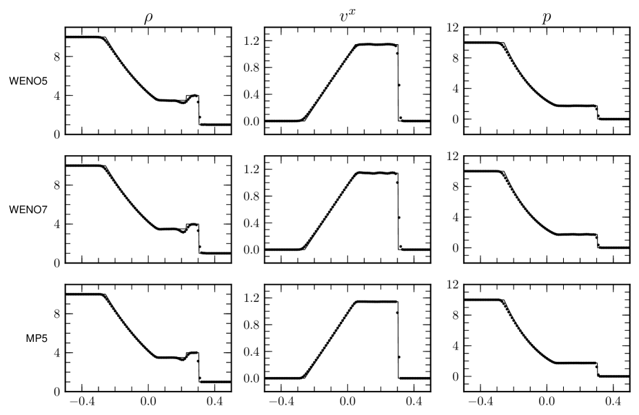
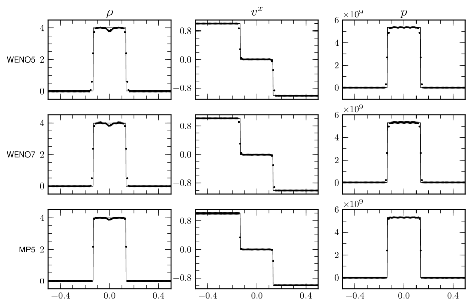
In Figure 1 we show with a solid line the analytic solution, while filled circles are used to represent the solution obtained at time $t=0.2$ with the different numerical schemes. The grid resolution is $\Delta^{1}=1/100$ and the timestep $\Delta^{0}=0.002$ for all the runs. Note that the numerical solution is not down-sampled and hence it corresponds to a genuinely coarse resolution. We do not show the results obtained with the bandwidth-optimised schemes since they are basically indistinguishable from the ones obtained using their traditional counterpart, i.e. the solution obtained with WENO3B is basically on top of the one obtained with WENO5 and the solution obtained with WENO4B is identical, at the plot scale, with the one obtained with WENO7. Since the results obtained with the bandwidth-optimized schemes are found to be very close to the ones obtained with the standard WENO schemes in all the shock-tube test that we performed, we will show only the numerical solutions obtained with WENO5, WENO7 and MP5 in all the cases.

Figure 2: The same as in Figure 1, but for the Newtonian blast-wave test. The resolution is $\Delta^{1}=1/100$ and the timestep is $\Delta^{0}=0.0001$ for all the runs.

Even at this fairly low resolution, all the schemes are able to capture well both the shock wave and the rarefaction wave, showing the good behaviour of our entropy fix. The shock wave is captured within three gridpoints. There are no appreciable post-shock oscillations in the solution obtained with the MP5 reconstruction, while small oscillations are present in the velocity field with WENO5 and, in particular, with WENO7.

We note that the contact discontinuity is resolved, but not without oscillations. However, we should bear in mind that, although the density contrast is small across the contact discontinuity, this test is a severe one due to the high Mach number of the shock wave, i.e. $\mathcal{M}_{s}\approx 360$.

3.1.2 Blast wave

The second test is similar to the first one, but results in a much larger density contrast at the contact discontinuity. The initial data is given by

$$(\rho_{L},v_{L},p_{L})=(10^{-3},0,1)\,,\quad (\rho_{R},v_{R},p_{R})=(10^{-3},0,10^{-5})\,,$$ (34)

and the adiabatic index is still $\Gamma=5/3$. Also in this case, the analytic solution consists in a right-going shock wave, followed by a contact discontinuity and a left-going rarefaction wave.

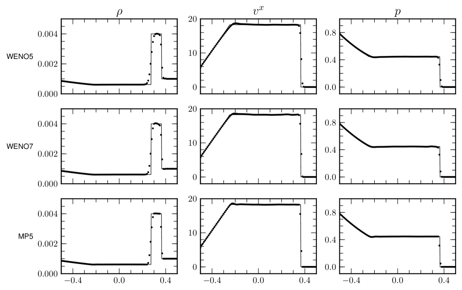
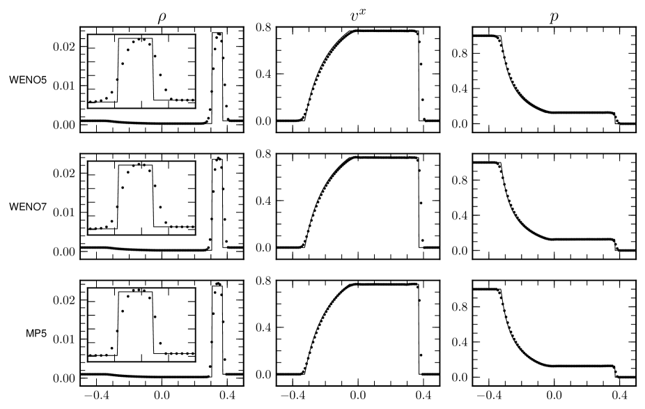
In Figure 2 we show the exact solution at time $t=0.015$ (solid line), as well as the numerical solution (filled circles) obtained using different numerical schemes. The grid resolution is $\Delta^{1}=0.01$ ($N=100$) and the timestep is $\Delta^{0}=0.0001$ for all the runs. The Mach number of the shock wave is $\mathcal{M}_{s}\approx 190$ and in this case all our schemes are free from major oscillations. The shock wave is resolved within two grid points, while the contact discontinuity is smeared over 5-6 grid points.

The MP5 scheme is able to properly capture the constant state between the shock wave and the contact discontinuity, while the WENO schemes result in more “rounded” solutions. In particular both WENO5 and WENO7 overestimated the density contrast.

Figure 3: The same as in Figure 1, but for the Newtonian rotated Sod test. The resolution is $\Delta^{i}=1/200$ and the timestep is $\Delta^{0}=0.000625$ for all the runs.

3.1.3 Rotated Sod test

A genuinely three-dimensional shock-tube test in Newtonian hydrodynamics is offered by the classical rotated Sod test (Sod 1978). In this case, the adiabatic index is $\Gamma=1.4$ and the right and left states are

$$(\rho_{L},v_{L},p_{L})=(1,0,1)\,,\quad (\rho_{R},v_{R},p_{R})=(0.125,0,0.1)\,,$$ (35)

the initial, 1D data, is rotated by $45^{\circ}$ about the $z$ and $y$ axes to yield a shock wave that is diagonal to the principal axes of the grid. The analytic solution consists in a left-going rarefaction wave and a right-going shock wave separated by a right-going contact discontinuity.

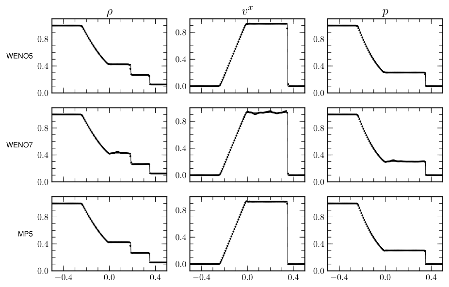
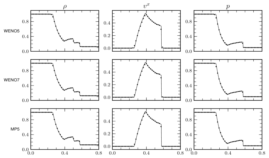
In Figure 3 we show the analytic solution in the diagonal direction (solid line), as well as the numerical solutions (filled circles), at time $t=0.2$. The spatial resolution is $\Delta^{i}=1/200$ for $i=1,2,3$ and the timestep is $\Delta^{0}=0.000625$ for all the runs. All the schemes are able to properly capture the main features of the solution: the discontinuities are captured within 1 or 2 gridpoints and both WENO5 and MP5 are able to capture the plateau in the velocity. The solution obtained with the WENO7 scheme presents oscillations in the velocity after the shock wave and in the density and pressure fields downstream the contact discontinuity. Similar oscillations are also observed with WENO5 and MP5 when the resolution is halved.

Overall, these tests demonstrate the accuracy of the dimensionally unsplit approach that we use to treat the multi-dimensional case.

Figure 4: Isocontours of the rest-mass density at time $t=0.2$ for the Newtonian double Mach reflection test, obtained with different schemes. We show 20 contours levels equally spaced between 0 and 3. The resolution is $\Delta^{i}=1/480$ and the timestep is $\Delta^{0}=1/40000$ for all the runs.

3.1.4 Double Mach reflection test

A final test in Newtonian hydrodynamics is the double-Mach reflection test proposed by Woodward & Collela (1984). The initial data describes a right-going Mach 10 shock wave making a $60^{\circ}$ angle with the computational grid and intersecting the $x-$axis at $x=1/6$. A perfectly reflecting wall is placed along the $x-$axis in the $x>1/6$ region, while the values along the other regions of the boundary are set to the pre and post-shocked values on the left/right side of the shock wave [see Woodward & Collela (1984) for details on the boundary conditions and the initial data].

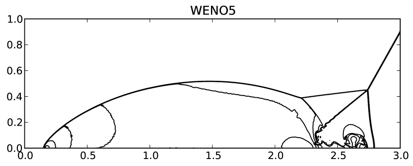
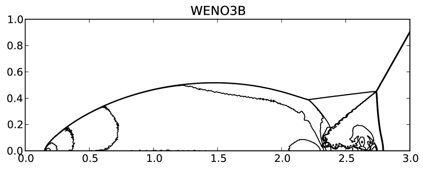
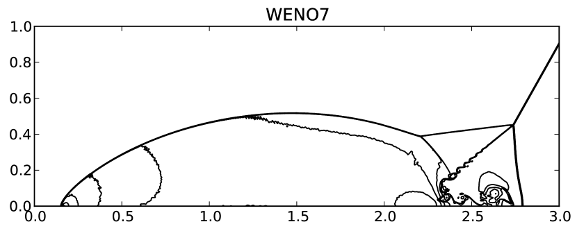
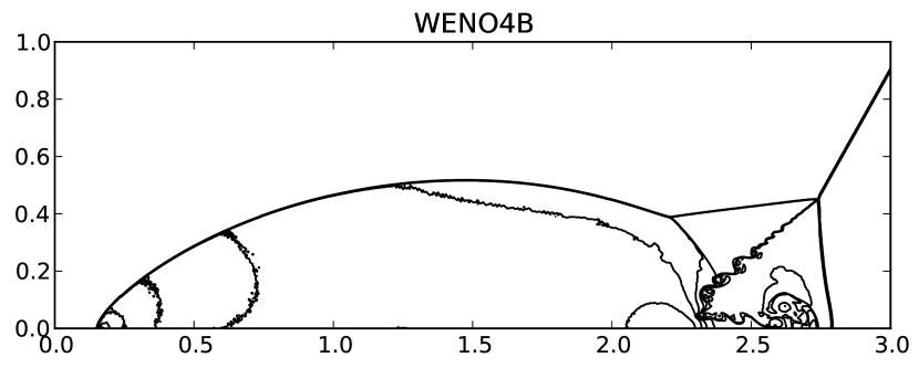
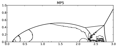
We considered the numerical solutions obtained with WENO5, WENO7, MP5, WENO3B and WENO4B in the computational domain $0\leq x\leq 4$, $0\leq y\leq 1$. For each of these schemes we performed five runs with resolutions $120\times 30$, $240\times 60$, $480\times 120$, $960\times 240$ and $1920\times 480$. In Figure 4 we show isocontours (with an equal spacing of 0.15 between 0 and 3) of the rest-mass density obtained at the highest resolution at time $t=0.2$ by the different numerical schemes. In order to ease the comparison with the results reported in Woodward & Collela (1984), we show only the region $x<3$.

Our code performs well in this test across all the reconstruction schemes that we tried. All the discontinuities, including the contact discontinuity ahead of the jet region, are well resolved within few grid regions, even at the lowest resolution. As we increase the number of gridpoints we do not observe any sign of the carbuncle phenomenon and this seems to be an indication that our algorithm is able to introduce enough numerical dissipation to avoid the odd-even decoupling.

At high-enough resolution it is possible to observe the development of instabilities upstream from the reflected shock wave, generating small scale structures along the contact discontinuity. The ability of the different codes to resolve these structures can be used as an indication of their numerical viscosity. In particular we can see how the bandwidth-optimized schemes gain with respect to their “standard” counterparts. For instance, WENO3B, which uses the same stencil as WENO5, yields a solution which is in qualitative agreement with the one obtained using WENO5 at twice the spatial resolution. The same is also true if we compare WENO4B and WENO7.

All things considered, we find that the best performance is given by the MP5 scheme. This algorithm has a computational cost which is comparable with the one of WENO5, as it uses the same stencil. Nevertheless the solution obtained with MP5 is very close to the one obtained with the optimized WENO4B scheme, which, in 3D, is almost twice as expensive as WENO5.

3.2 Special-relativistic hydrodynamics

In this Section we will present the results obtained in a series of tests in special-relativistic hydrodynamics.

Figure 5: Analytic solution and numerical solution computed with WENO3B with $50$ gridpoints for the case of an smooth wave in an adiabatic relativistic fluid. The figure shows both the initial data (top panel) and the solution at time $t=0.8$ (bottom panel). The solid line represent the analytic solution, while the filled circles represent the numerical one.

3.2.1 Adiabatic smooth flow

The first test we present is designed to show the accuracy of the code in the case of smooth solutions and hence to measure rigorously the convergence order of THC for the different schemes implemented. This test is very similar to the one discussed by Zhang & MacFadyen (2006).

We consider a one-dimensional, large-amplitude, smooth, wave propagating in an isentropic fluid, with polytropic equation of state,

$$p=K\rho^{\Gamma},$$ (36)

where $K=100$ and $\Gamma=5/3$. The rest-mass density at $t=0$ is given by

$$\rho_{0}(x)=\begin{cases}1+\exp\left[-1/(1-x^{2}/L^{2})\right]\,,&\textrm{if }|x|<L;\\ 1,&\textrm{elsewhere};\end{cases}$$ (37)

where, differently from Zhang & MacFadyen (2006), the initial profile of the rest-mass density is chosen to be $C^{\infty}$ but is not analytic. We have found this choice important to obtain the correct convergence order at very high resolutions. Indeed, when adopting the same profile as in Zhang & MacFadyen (2006), we found that the jump discontinuity in the fifth derivative of the initial data prevents the WENO7 scheme from achieving a convergence order larger then five. Besides this small difference, our initial data is basically identical to the one used by Zhang & MacFadyen (2006). The initial velocity is setup assuming that one of the two Riemann invariants (Anile 1990),

$$J_{-}=\frac{1}{2}\ln\left(\frac{1+v}{1-v}\right)-\frac{1}{\sqrt{\Gamma-1}}\ln\left(\frac{\sqrt{\Gamma-1}+c_{s}}{\sqrt{\Gamma-1}-c_{s}}\right)\,,$$ (38)

where $c_{s}$ is the sound speed, is constant in the whole region and so that $v=0$ if $|x|\geq L$. The other Riemann invariant,

$$J_{+}=\frac{1}{2}\ln\left(\frac{1+v}{1-v}\right)+\frac{1}{\sqrt{\Gamma-1}}\ln\left(\frac{\sqrt{\Gamma-1}+c_{s}}{\sqrt{\Gamma-1}-c_{s}}\right)\,,$$ (39)

is not constant, so that the initial data describes a right-going wave.

The analytic solution can be easily found in Lagrangian coordinates, up to the caustic point, using the method of characteristics (Anile 1990), while its calculation in Eulerian coordinates involves the solution of a transcendental equation. For the purposes of our calculation, a good-enough approximation of the exact solution was obtained by computing it on a very fine Lagrangian grid (we have used $100,000$ gridpoints), and interpolated on the Eulerian grid using a cubic spline interpolation. This solution is then used as the reference solution against which the numerical solutions obtained with THC have been compared.

In our test we set $L=0.3$ and use a computational grid in the region $-0.4\leq x\leq 2$, evolving the initial data up to time $t=1.6$, which is approximately the time when a caustic appears and the solution becomes discontinuous. We performed this test using different schemes and different resolutions and we measured the $L^{1}-$norm of the error against the reference solution. Differently from all the other tests, instead of the third-order SSP-RK scheme, we adopt here a fourth-order RK time integrator. The reason for this choice is that, since this test involves a smooth solution, a SSP time-integrator is not required. Moreover, as we will show in the following, the use of a more accurate time integrator enabled us to measure a convergence order of the spatial discretization which is not spoiled by the order in time, the only exception being the highest resolution run done with WENO7. The CFL factor is set to be $C\approx 0.2$.

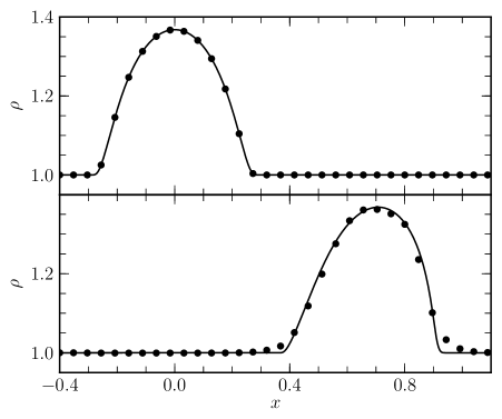
The initial rest-mass density profile. as well as the solution at time $t=0.8$, which we take as a reference time for the measure of the error, is shown in Figure 5, together with the solution obtained with WENO3B using $50$ gridpoints. As it can be seen from the Figure, the solution at the considered time is still smooth and our scheme is able to properly capture it very well even at this very coarse resolution.

Figure 6: $L^{1}-$norm of the error for different resolutions and for different numerical schemes for the case of a smooth simple wave in an adiabatic relativistic fluid

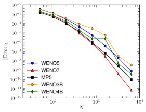
The $L^{1}-$norm of the error, as measured at the reference time, is shown in Figure 6. The first thing one notices is that all our schemes approach the expected convergence order only asymptotically, at very high resolution. The reason for this behaviour is in the “kinks” ahead and behind the pulse, where the numerical error is largest. These regions are “misinterpreted” as discontinuities by the shock-detection part of our schemes, unless they are resolved with enough gridpoints.

The best performing scheme in this test is the MP5 one: at low resolution it yields a smaller error then the seventh-order WENO scheme, which, in turn, is able to attain an higher convergence order only at a resolution which is unfeasible in any practical multidimensional applications. The bandwidth optimized schemes present a somewhat errant behaviour in their convergence order, with WENO4B, not even showing a monotone trend in $L^{1}-$norm of the error as a function of the number of gridpoint. We do not presently have an explanation we find sufficiently convincing for the behaviour shown.

Figure 7: Order of convergence, as measured using the two highest resolution runs, as a function of the time to the caustic for different numerical schemes for the smooth simple wave test.

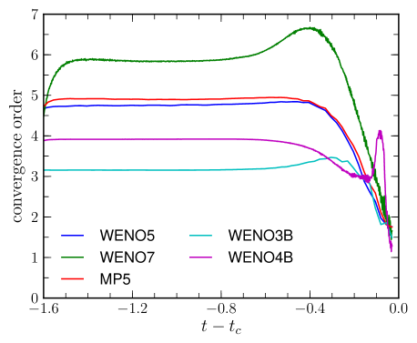
Finally it is interesting to study the convergence order of the different numerical schemes as a function of $t-t_{c}$, where $t_{c}$ is the time when the caustic is formed. The convergence order is computed using the error with respect to the exact solution of the two highest resolution runs and is shown in Figure 7. At these very high resolutions, all the schemes appear to be converging at their nominal converge order away from the caustic, apart from WENO7 that appears to have already reached saturation. Its order of convergence increases up to almost seven close to the caustic, at time $t-t_{c}\approx-0.4$, because there the error is dominated by the presence of a more steep gradient ahead of the pulse. Before that, the error from the spatial discretization is probably very close to the one from the time discretization (we recall that we use a fourth-order RK integrator), thus degrading the convergence order.

Indeed, as the time of shock formation approaches, the order of the schemes decreases slowly to the first-order expected in the case of discontinuities. The bandwidth optimized schemes and, in particular, WENO4B show, again, an erratic behaviour of their convergence order. The reasons for this behaviour are most probably the same ones behind the similar behaviour observed while looking at the error as a function of the number of gridpoints.

Figure 8: The same as in Figure 1, but for the relativistic blast-wave test. The resolution is $\Delta^{1}=1/400$ and the timestep is $\Delta^{0}=0.0005$ for all the runs.

3.2.2 Blast wave

When contrasted with its Newtonian counterpart, one of the most striking features of relativistic hydrodynamics is that relativistic fluids can exhibit much stronger shock waves. For this reason, it is important to assess the capability of the code to handle very strong shocks. As a first example we consider a one-dimensional shock-tube where the initial data is given by,

$$(\rho_{L},v_{L},p_{L})=(10^{-3},0,1)\,,\quad (\rho_{R},v_{R},p_{R})=(10^{-3},0,10^{-5})\,,$$ (40)

and the adiabatic index is still $\Gamma=5/3$. This initial data is formally identical to the one used in Section 3.1.2 in the Newtonian case. The analytic solution consists again in a transonic left-going rarefaction wave and in a right-going shock wave separated by a right going contact discontinuity. The shock wave has a relativistic Mach number $\mathcal{M}_{s}\approx 50$ (Chiu 1973; Konigl 1980).

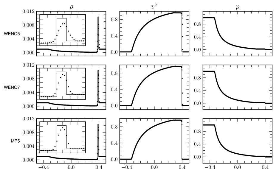
The results obtained with the different numerical schemes are reported in Figure 8, where we show the analytic solution (solid line) as well as the numerical ones (filled circles) obtained with WENO5, WENO7 and MP5, at time $t=0.4$. As in the Newtonian case, we do not show the results obtained with the bandwidth optimized schemes as they are basically identical to the ones of their traditional variant. The spatial resolution that we use is $\Delta^{1}=1/400$ and the CFL factor is $C=1/5$ in all cases.

Figure 9: The same as in Figure 1, but for the relativistic shock-heating test. The resolution is $\Delta^{1}=1/100$ and the timestep is $\Delta^{0}=0.001$ for all the runs.

The CFL factor in this test is basically constrained by the MP5 scheme: while the WENO schemes appear to be robust and stable up to CFL factor of $C\approx 2/5$, the MP5 algorithm produces large oscillations and yields non-physical values in the conservative variables unless a smaller CFL factor is used. We point out that for this particular test the necessity of using small timesteps to avoid the creation of unphysical states has been observed also when using other numerical schemes. For instance, when using the finite-volume code Whisky (Baiotti et al. 2003, 2005), with the HLLE approximate Riemann solver [see, e.g. Toro (1999)] and the PPM reconstruction (Colella & Woodward 1984), the maximum allowed CFL factor was also found to be $C\approx 2/5$. It is also known that, for the monotonicity-preserving property to hold for the MP5 scheme, the timestep must be subject to an additional constraint which is distinct from the standard CFL condition (Suresh & Huynh 1997). Yet, it is somewhat surprising to observe that MP5 requires a timestep which is smaller by a factor of order two with respect to the WENO schemes. Furthermore, this property does not seem to be a peculiarity of this specific problem, since we observed a similar behaviour also for the other tests that we performed.

Zhang & MacFadyen (2006) report that the use of MP5 reconstruction results in large numerical oscillations in their special relativistic code. In our code, we see a similar behaviour unless we use a timestep which is about half of the one considered “safe” for the WENO scheme. If the timestep is sufficiently small, on the other hand, the MP5 algorithm results in very accurate solutions, as in the Newtonian case. In particular in Figure 8 we can see the results obtained with this particular test. Our code, with MP5, is able to capture the shock wave within three gridpoints while the contact discontinuity is spread across six points. WENO7 yields a solution of similar quality, while WENO5 is slightly more diffusive.

The capability of a numerical code to capture the density contrast for this particular test is a classical benchmark for relativistic hydrodynamics codes. Again, using as reference the Whisky code, the use of the HLLE solver with PPM reconstruction and with artificial compression, leads to a maximum density which is $71\%$ of the analytic solution. At the same resolution, our THC using a WENO5, WENO7 and MP5 reconstruction is able to attain a maximum density which is respectively $78\%$, $90\%$ and $91\%$ of the analytical value. These results are in very good agreement with the ones reported by Zhang & MacFadyen (2006), who measured a relative value of $72\%$ and $79\%$ for their implementation of PPM and WENO5 schemes.

3.2.3 Shock-heating

An even more striking example of how relativistic effect can enhance the density contrasts in shock waves is given by the classical shock-heating test. In this case, the initial data is given by

$$(\rho_{L},v_{L},p_{L})=(10^{-3},v,10^{3})\,,\quad (\rho_{R},v_{R},p_{R})=(10^{-3},-v,10^{3})\,,$$ (41)

the polytropic index is $\Gamma=4/3$ and

$$v=\sqrt{1-\frac{1}{W^{2}}}\simeq 0.99999949\,,$$ (42)

where the Lorentz factor is set to be $W=1000$. In this case, the analytic solution is represented by two shocks whose collision compresses the fluid, converting its kinetic energy into thermal energy, that is, through a “shock heating”.

In Newtonian hydrodynamics the maximum compression ratio can be computed as

$$\sigma_{\mathrm{newt}}=\frac{\Gamma+1}{\Gamma-1}=7\,,$$ (43)

for all the values of $v$, while it is easy to show (Martí & Müller 2003) that in the relativistic case the compression ratio is

$$\sigma=\frac{\Gamma+1}{\Gamma-1}+\frac{\Gamma}{\Gamma-1}(W-1)\simeq 4003\,,$$ (44)

thus about three orders of magnitude larger for the same adiabatic index and growing linearly with the Lorentz factor.

The exact solution at time $t=0.4$, as well as the numerical solutions obtained with our code, are shown in Figure 9. As it can be seen from the Figure, THC is able to handle very well this large compression ratio. The WENO5 and WENO7 solutions are affected by some small wall-heating effect (Noh 1987; Rider 2000), resulting in a slight under-density near $x=0$ and some numerical oscillations in the pressure. The MP5 scheme, on the other hand, yields a solution which is essentially free from oscillations in the pressure and much less affected by the wall-heating effect in the density variable, although at the cost of a smaller timestep, as discussed in the previous Section.

Figure 10: The same as in Figure 1, but for the relativistic blast-wave test. The resolution is $\Delta^{1}=1/100$ and the timestep is $\Delta^{0}=0.002$ for all the runs.

3.2.4 Transverse shock

Another peculiar difficulty of relativistic hydrodynamics and without a Newtonian counterpart, is that the equations for the momentum in the different directions are coupled together by the Lorentz factor: even in one-dimensional problems the application of a transverse velocity can change completely the solution. This feature was first pointed out by Pons et al. (2000) and Rezzolla & Zanotti (2002), and then used by Rezzolla et al. (2003) and Aloy & Rezzolla (2006) to discover new physical effect [see also Mignone et al. (2005); Zhang & MacFadyen (2006) for a description of the numerical consequences of this property].

To explore the flow dynamics in this case, we consider the same initial data as for the blast-wave test [see Section 3.2.2], with the only difference that we add a transverse velocity to the initial data, i.e.

$$v^{t}_{L}=0\,, v^{t}_{R}=0.99\,.$$ (45)

As discussed in Zhang & MacFadyen (2006) this is not a very challenging test, since the velocity is added only to the cold fluid and it does not interact with the contact discontinuity. Nevertheless it is a good test to evaluate the capability of the code to handle the presence of a transverse-velocity at a moderate resolution, while more extreme configurations require a resolution which is unreasonably high for multi-dimensional applications to obtain decent solutions. A way around this issue is the use of adaptive-mesh-refinement (AMR) (Zhang & MacFadyen 2006), which however would not be useful for our use of THC to study of relativistic turbulence Radice & Rezzolla in prep. (it is in fact debatable whether the use of AMR is advantageous in this case).

In Figure 10 we show the analytic and numerical solutions for this problem at time $t=0.4$. The presence of the transverse velocity widens the state between the shock wave and the contact discontinuity. The density contrast is also smaller with respect to the case where no tangential velocity is present. THC is able to capture the solution even at the low resolution, $\Delta^{1}=1/100$, shown in the Figure. The MP5 scheme overestimates slightly the density contrast, but all of the algorithms are able to capture the correct location of the shock wave.

Figure 11: Rest-mass density (left panels) velocity (middle panels) and pressure (right panels) for the relativistic spherical explosion test. We show the results obtained with different schemes (dotted) as well as a reference solution (solid line) obtained with the 1D spherically symmetric code EDGES, Radice & Rezzolla (2011), using 2000 elements of degree 3. The resolution is $\Delta^{i}=1/100$ and the timestep is $\Delta^{0}=0.00125$ for all the runs.

3.2.5 Spherical explosion

As an example of a test involving non-grid-aligned shocks we consider the classical test of the spherical explosion in relativistic hydrodynamics. The initial data in this case is given by

$$(\rho,v,p)=\begin{cases}(1,0,1)\,,&\textrm{if }r<0.4\,;\\ (0.125,0,0.1)\,,&\textrm{elsewhere}\,.\end{cases}$$ (46)

Since no analytic solution is known in this case, we use as reference solution the one computed using the one-dimensional spherically-symmetric discontinuous-Galerkin code EDGES (Radice & Rezzolla 2011) using 2000 elements of degree 3, solid lines, and compare it with the numerical solutions obtained in three-dimensions with THC in the diagonal direction. Both solutions at time $t=0.25$ are shown in Figure 11, when using a resolution $\Delta^{i}=1/100$ and a timestep $\Delta^{0}=0.00125$ for all the numerical schemes. As in the one-dimensional case, a small timestep is necessary in order to avoid numerical oscillations with the MP5 algorithm, while the other schemes appear to be stable even with a timestep which is twice as large.

Overall, all the schemes are able to properly capture the reference solution even at this very low resolution: the contact discontinuity is captured within two grid points and no oscillations are found in any of the physical quantities.

Figure 12: RMS value of the $y$-component of the velocity during the linear-growth phase of the 2D relativistic Kelvin-Helmholtz instability, for different numerical schemes. The solid lines represent the results obtained at the highest resolution, $1024\times 2048$, while the dashed lines represent the results obtained at the lowest resolution, $128\times 256$. The timestep is chosen so that the CFL factor is $C\approx 0.25$ for all of the runs.

Figure 13: Rest-mass density for the 2D relativistic Kelvin-Helmholtz instability test at time $t=3$ and for different numerical schemes. The resolution is $512\times 1024$ for all the schemes and the CFL factor is $C\approx 0.25$. This figure should be compared with its equivalent Figure 20 presented in Appendix A and at a resolution $1024\times 2048$

3.2.6 Kelvin-Helmholtz instability in 2D

The last test that we present is a classical benchmark for multidimensional hydrodynamics codes: the simulation of the KHI in two-dimensions, $x,y$. In order to ease the comparison with the existing literature, the initial conditions are chosen following Beckwith & Stone (2011). The shear velocity is given by

$$v^{x}(y)=\begin{cases}V_{\mathrm{shear}}\tanh\left[(y-0.5)/a\right]\,,&\textrm{if }y>0\,;\\ V_{\mathrm{shear}}\tanh\left[(y+0.5)/a\right]\,,&\textrm{if }y\leq 0\,;\end{cases}$$ (47)

where $a=0.01$ is the characteristic size of the shear layer and $V_{\mathrm{shear}}=0.5$, corresponding to a relative Lorentz factor, i.e. the Lorentz factor of a part of the fluid as seen by an observer comoving with the other one, of $W=2.29$. The instability is seeded by adding a small perturbation in the transverse component of the velocity,

$$v^{y}(x,y)=\begin{cases}A_{0}V_{\mathrm{shear}}\sin(2\pi x)\exp\left[-\left({y-0.5}\right)^{2}/\sigma\right]\,,&\textrm{if }y>0\,;\\ -A_{0}V_{\mathrm{shear}}\sin(2\pi x)\exp\left[-\left({y+0.5}\right)^{2}/\sigma\right]\,,&\textrm{if }y\leq 0\,;\end{cases}$$ (48)

where $A=0.1$ is the perturbation amplitude and $\sigma=0.1$ its characteristic lengthscale. The adiabatic constant is $\Gamma=4/3$ and the initial pressure is uniform, $p=1$. The rest-mass density distribution, which is uniform in the $x$-direction, is instead given by

$$\rho(y)=\begin{cases}\rho_{0}+\rho_{1}\tanh\left[(y-0.5)/a\right]\,,&\textrm{if }y>0\,;\\ \rho_{0}-\rho_{1}\tanh\left[(y+0.5)/a\right]\,,&\textrm{if }y\leq 0\,;\end{cases}$$ (49)

where $\rho_{0}=0.505$ and $\rho_{1}=0.495$, so that $\rho=1$ in the regions with $v^{x}=0.5$ and $\rho=0.1$ in the regions with $v^{x}=-0.5$. Finally the computational domain is $-0.5\leq x\leq 0.5$, $-1\leq y\leq 1$ and we use periodic boundary conditions in all the directions. Differently from Beckwith & Stone (2011) we do not add a random perturbation to the initial data and we do not take into account the effects of magnetic fields. Nevertheless, our results are in good agreement with the ones by Beckwith & Stone (2011) in the linear phase of the instability, since the magnetic field that they use is too weak to play a dynamical role in this phase.

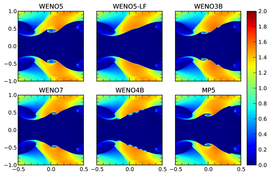
We performed a series of simulations using six different numerical schemes: WENO5, WENO7, MP5, the bandwidth optimized WENO3B, WENO4B and using the WENO5 scheme, but with the Lax-Friedrichs flux-split, WENO5-LF. For each of these schemes, we ran with four different resolutions: $128\times 256$, $256\times 512$, $512\times 1024$ and $1024\times 2048$. For all the runs, the CFL factor was taken to be $C\approx 0.25$.

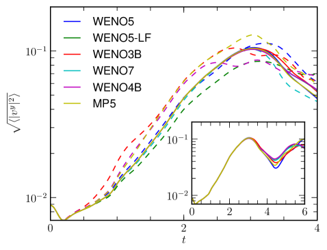
The first quantity of interest to check is the growth rate of the transverse velocity during the linear-growth phase of the KHI, as computed with the different numerical schemes. This can be done by comparing the evolution of the root-mean-square (RMS) value of the transverse component of the velocity and defined as

$$\langle|v^{y}|^{2}\rangle\equiv\frac{1}{V}\int_{V}|v^{y}|^{2}\,dV\,,$$ (50)

where $V$ is the volume of the computational domain. This is shown in Figure 12, where, for each numerical scheme, we show the results taken at the lowest resolution (dashed lines) and at the highest one (continuous lines). First, we notice that with our setup the linear-growth phase of the instability lasts up to until $t\simeq 3$. At that time, in fact, the transverse velocity reaches saturation and afterwards the fluid starts to become turbulent and the velocity shows large fluctuations.

Mignone et al. (2009) showed the importance of including the contact wave in the approximate Riemann solver in the case of a finite-volume code. In particular, they observed that while the growth rate of $v^{y}$ was already accurate at low resolution when using their HLLD Riemann solver, in the cases where the more dissipative HLLE Riemann solver was employed the correct growth rate was recovered only at high resolution [similar results were also reported by Beckwith & Stone (2011)]. In analogy with what is observed with finite-volume codes, we also remark the importance of avoiding excessive dissipation in the contact discontinuity by comparing the results obtained with the Lax-Friedrichs and the Roe flux-split when using WENO5. The Lax-Friedrichs flux-split underestimates the growth rate at low resolution and achieves a good accuracy in its measure only at resolution $256\times 512$ (not shown in the figure). WENO5 and WENO7 with the Roe flux split already have a growth rate which is consistent with the highest resolution runs at the lowest resolution of $128\times 256$.

The behaviour of the MP5 scheme, as well as the one of the bandwidth-optimized WENO schemes, is more surprising: all of these schemes overestimate the growth of the RMS transverse velocity at low resolution. This problem disappears as we increase the resolution and in the $256\times 512$ the growth rate is already consistent with the highest-resolution one for all the numerical schemes.

Some insight about the numerical viscosity can be gained by looking at the topology of the flow during the linear-growth phase of the KHI. In particular in Figure 13 we show a colour map of the rest-mass density obtained with the different schemes at time $t=3$ using the $512\times 1024$ resolution. Mignone et al. (2009) noticed that their solution obtained with the HLLD Riemann solver was showing a different structure, with the development of secondary small-scale instabilities along the shear layer, and that were not present when using the more diffusive HLLE solver. Similar differences were also observed in other works [see, e.g. Agertz et al. (2007); Springel (2010)], and the presence (or absence) of these secondary instabilities has been often used as an indication of the numerical viscosity of the codes. Beckwith & Stone (2011) interpret these differences as an indication that HLLE is converging to a different weak solution from HLLD. Since both solvers are entropic (i.e. with non-decreasing entropy), this would imply the non-uniqueness of the entropic solution for the Euler equations in this case.

In agreement with the conclusions of Beckwith & Stone (2011), we also note that these secondary instabilities, although only numerical artifacts (see below), appear only in schemes able to properly treat the initial contact discontinuity. As a result, the rest-mass density in Figure 13 obtained with WENO5 and WENO5-LF match very well the ones they obtained using HLLD and HLLE, respectively. However, our results do not support their conjecture that different schemes are converging to different weak solutions of the equations. The reason is that these secondary instabilities appear not to be genuine features of the solution and, rather, tend to disappear as the resolution is increased. For instance, the number of secondary vortices seems to change in a non-predictable fashion with the different numerical schemes and also with the resolution. This can be seen in Figure 13, which shows the great variability in the solutions obtained with different schemes. A similar variability is also present in results obtained at different resolutions with each scheme, WENO5-LF being the only exception. Finally, we point out that the size of the vortices is also shrinking as the resolution is increased. In essence, therefore, all of these considerations lead us to the conclusion that the secondary instabilities are triggered by the nonlinear dissipation mechanism of the different schemes, emerge neatly when computed with numerical schemes that treat properly the initial contact discontinuity, but do not have a physical meaning (see also the discussion in Appendix A).

A similar interpretation is also given by McNally et al. (2011), who go one step further and suggest to add additional viscosity to numerical codes displaying these secondary instabilities in order to prevent their growth. While the addition of extra dissipation is going to smooth out small scales numerical perturbations, we argue that this issue can only be resolved with the inclusion of physical viscosity. Artificial viscosity would probably compete with the internal, non-linear, dissipation mechanism of the schemes yielding results that would be even more difficult to interpret (as the viscous scale will now depend both on the resolution and on the artificial viscosity strength).

Figure 14: One dimensional power spectrum of the rest-mass density for the 2D relativistic Kelvin-Helmholtz instability test at time $t=3$ and for different numerical schemes. The resolution is $1024\times 2048$ for all the schemes and the CFL factor is $C\approx 0.25$.

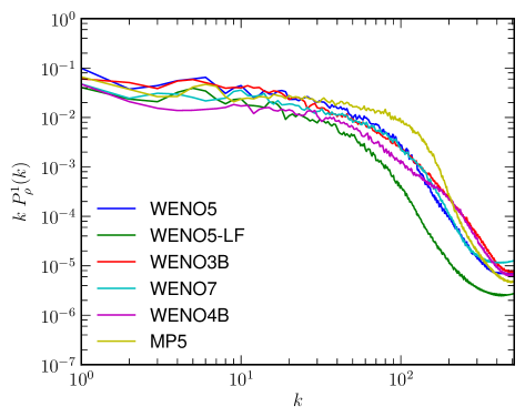
A more quantitative way of estimating the numerical viscosity of the code in this test has been proposed by Beckwith & Stone (2011) and is based on the study of one-dimensional integrated power-spectra. Given a quantity $u(x,y)$ we define its integrated power-spectrum

$$P^{1}_{u}(k)=\int_{-1}^{1}|\hat{u}(k,y)|^{2}dy\,,$$ (51)

where $k$ is the wavenumber and

$$\hat{u}(k,y)=\int_{-1/2}^{1/2}u(x,y)e^{-2\pi ikx}dx\,,$$ (52)

is the one-dimensional Fourier transform of $u$. To ease the comparison with the spectra reported by Beckwith & Stone (2011), the power spectrum is then normalized so that

$$\sum_{k=1}^{N/2}P^{1}_{u}(k)=1\,,$$ (53)

where $N$ is the number of gridpoints. The one-dimensional power spectrum can be used to quantify the typical scale of structures, such as the secondary vortices discussed above, stretched in the direction of the bulk shear flow.

In Figure 14 we show the spectra of the rest-mass density for the different schemes at time $t=3$ and for the highest resolution. As expected the WENO5-LF scheme stands out as the scheme having the largest dissipation. More surprising is the behaviour of the bandwidth optimized schemes: they appear to be improving over their classical counterparts only at high wavenumbers, that is, at scales that are dominated by the (non-physical) dissipation of the scheme. Even more unexpected is the ability of the MP5 scheme to resolve small scales structures and that, on the basis of the argument about the development of the secondary instabilities, should be more dissipative than WENO4B, but which instead appears to yield more small-scale structures in the rest-mass density.

A similar conclusion can be obtained by studying the spectrum of the kinetic energy

$$E_{k}=\rho W(W-1)\,,$$ (54)

but which we do not report since its behaviour is very similar to the one shown for the rest-mass density.

4 The relativistic Kelvin-Helmholtz instability in 3D

As an example of a non-trivial application of THC and a perfect playground to evaluate the performances of the different numerical schemes for the simulation of turbulence reported in Radice & Rezzolla in prep., we present here a study of the relativistic turbulence generated by the KHI in three-dimensions. Our analysis is not meant to be a systematic assessment of the accuracy of these methods for direct numerical simulations of compressible relativistic turbulence, as done, for instance by Kitsionas et al. (2009), or Johnsen et al. (2010) in the case of classical turbulence. Rather, our analysis is meant to assess how the different methods reproduce the same turbulent initial-value problem and to provide some insight on the spectral properties of the different schemes.

The relativistic KHI [see, e.g. Bodo et al. (2004)] is of particular interest because of its relevance for the stability of relativistic jets [see, e.g. Perucho et al. (2007, 2010)], and because of its potential role in the amplification of magnetic fields in gamma-ray bursts [see, e.g. Zhang et al. (2009)], and binary neutron-star mergers (Baiotti et al. 2008; Giacomazzo et al. 2009; Obergaulinger et al. 2010; Rezzolla et al. 2011).

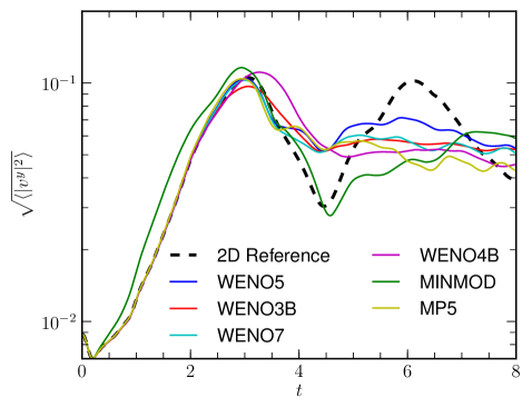
We consider a triply-periodic box, $-0.5\leq x\leq 0.5$, $-1\leq y\leq 1$, $-0.5\leq z\leq 0.5$. The initial conditions are the same ones employed in Section 3.2.6, and the symmetry in the $z$-direction is broken with the application of random perturbations, uniformly distributed in the range $[0,0.01]$, applied to the velocity in the $z$-direction $v^{z}$. We simulated this system up to the time $t=30$ on a grid of $256\times 512\times 256$ cells using the WENO5, WENO7, MP5, WENO3B and WENO4B reconstructions. In addition, we have also performed one run at the same resolution using the second-order MINMOD reconstruction. Furthermore, because of the high computational costs involved to check the convergence of the code, we have managed to run only one model at twice the reference resolution, i.e. $512\times 1024\times 512$, using the WENO5 reconstruction scheme.

As discussed in the previous Section, the MP5 scheme requires a timestep which is half that of the other schemes. On the other hand, there is no need to run the WENO schemes with such a small timestep and in any “real” application we will run the WENO scheme with the maximum possible timestep. For this reason, and since we are interested in the performance of the different schemes in their “real-world” configuration,, we have not used the same CFL factor for all of them, with a considerable saving in computational costs. In particular, for all the runs we have used a CFL factor $C\approx 0.25$, with the exception of the one with the MP5 scheme, where we have used $C\approx 0.125$.

Figure 15: RMS value of the $y$-component of the velocity during the linear-growth phase of the 3D relativistic Kelvin-Helmholtz instability, for different numerical schemes. The thick-dashed line represent the results obtained at the highest resolution, $1024\times 2048$, in 2D with WENO5. The resolution is $256\times 512\times 256$ for all the schemes.

4.1 The linear evolution of the instability

First of all, we consider the evolution of the instability during its linear-growth phase. At this stage, the velocity perturbations in the direction perpendicular to the shearing one is growing exponentially and three-dimensional effects are still negligible.

The evolution of the RMS value of the $y$-component of the velocity is reported in Figure 15, where we show the results obtained with the different schemes, as well as a reference solution computed in two dimensions (2D) using WENO5 on $1024\times 2048$ grid points. As expected, all the numerical schemes, with the exception of MINMOD, are in very good agreement with the 2D solution up to the end of the linear-growth phase at time $t=3$, when 3D effects become important and turbulence starts to play an important role in the dynamics. It is interesting to note that MINMOD, which is the most dissipative of the schemes we are using, is actually overestimating the growth of the KHI. This suggests that some care should be taken when interpreting the results from under-resolved simulations, since it is not always safe to assume that the high numerical viscosity of the low-resolution runs tends to suppress the instability, yielding a lower-bound on its growth.

Figure 16: Rest-mass density in the $z=0$ plane for the 3D relativistic Kelvin-Helmholtz instability study at time $t=3$ and for different numerical schemes. The resolution is $256\times 512\times 256$ for all the schemes.

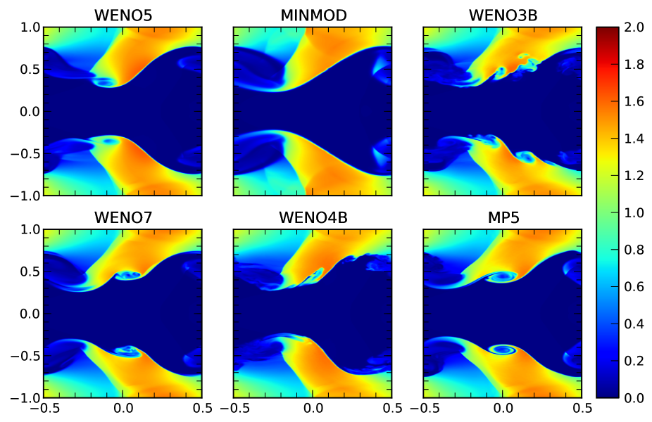
The rest-mass density at time $t=3$ is shown in Figure 16, where, in analogy with the 2D case, we find that the more dissipative schemes (i.e. MINMOD), do not show any sign of secondary instabilities apart from the seeded ones, while the least dissipative ones (i.e. WENO3B, WENO4B) show the emergence of secondary vortices.

At this point in time, the flow is still mostly two-dimensional, but it is interesting to notice the effects resulting from the small perturbations in the vertical velocity $v^{z}$. The perturbations have the same statistical properties in all the different models, but their effects are appreciably different for the different schemes, as can be seen from Figure 16. Although the perturbation in $v^{z}$ is random and it does not preserve any of the symmetries of the problem, it is still symmetric, on average, with respect to the $y$-axis. For this reason, one does not expect to find a large symmetry violation until the time when these perturbations have had enough time to grow and the dynamics has started to become dominated by three-dimensional effects. Yet, the optimized schemes WENO3B, WENO4B appear to be much more sensitive to the symmetry breaking than the others. The reason for this is probably that the bandwidth optimized-algorithms appear to trigger smaller-scale secondary instabilities, which, in turn, are more easily affected by the perturbations in the vertical velocity, since the perturbation does not average out at small scales.

Figure 17: Evolution of the concentration of the passive tracer in the $z=0$ plane for the 3D Kelvin-Helmholtz instability obtained using WENO5 on $512\times 1024\times 512$ gridpoints.

4.2 The nonlinear evolution of the instability

The linear-growth phase of the KHI instability ends when the primary vortices become unstable to secondary instabilities and the flow starts the transition to turbulence. At this point, three-dimensional effects start to become dominant and the dynamics is qualitatively different from the one observed in the 2D case.

In order to better track the evolution of the fluid in this phase, we monitor the concentration of a passive scalar field, $\phi$, transported with the fluid via the advection equation

$$\frac{\partial\phi}{\partial t}+\sum_{i=1}^{3}v^{i}\frac{\partial\phi}{\partial x^{i}}=0\,.$$ (55)

Equation (55) is not a conservation law, so that in can not be written directly in the form (1), but it is nevertheless a hyperbolic equation of the Hamilton-Jacobi type. For this reason, in order to solve numerically (55) we use a class of numerical schemes designed for this family of equations and that can be built using the non-oscillatory reconstruction of the derivative introduced in Section 2 [see, e.g. Shu (2007)]. In particular, the semi-discrete form of equation (55) becomes

$$\begin{split}\frac{d\phi_{i,j,k}}{dt}=&v^{x}_{i,j,k}\frac{\phi_{i-1/2,j,k}-\phi_{i+1/2,j,k}}{\Delta^{1}}+v^{y}_{i,j,k}\frac{\phi_{i,j-1/2,k}-\phi_{i,j+1/2,k}}{\Delta^{2}}+\\ &v^{z}_{i,j,k}\frac{\phi_{i,j,k-1/2}-\phi_{i,j,k+1/2}}{\Delta^{3}}\,,\end{split}$$ (56)

where $(\phi_{i-1/2,j,k}-\phi_{i+1/2,j,k})/\Delta^{1}$ is a high-order non-oscillatory approximation of $-\partial\phi/\partial x^{1}$ at $x_{i,j,k}$ obtained using an upwind-biased reconstruction, i.e.

$$\phi_{i-1/2,j,k}=\phi^{\pm}_{i-1/2,j,k},\qquad\textrm{if }v^{x}\lessgtr 0\,.$$ (57)

The “fluxes” in the other directions are obviously computed in an analogous way.

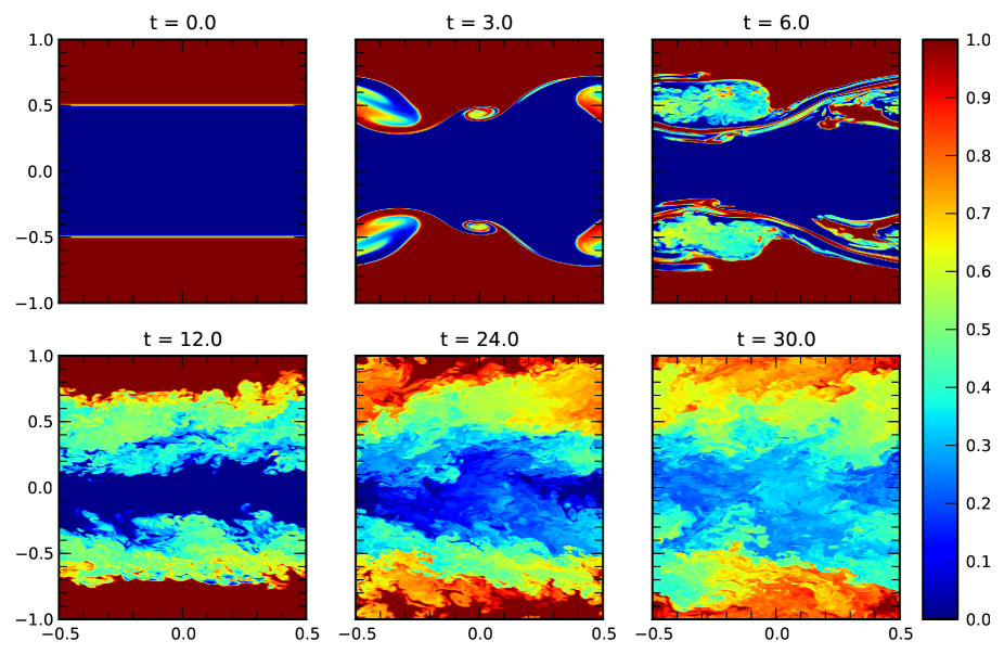
The time evolution of the tracer, as computed with WENO5 at the highest-resolution is shown in Figure 17. At the initial time, we set the scalar field $\phi$ to be equal to the rest-mass density, so that the initial configuration consists in two regions with opposite “colour”, separated by a thin transition layer. At the end of the linear regime, i.e. at time $t\simeq 3$, the tracer profile is distorted by the presence of the primary vortices as well as of the secondary ones, but there is only a marginal mixing of the two “phases” of the fluid. Note that, since we do not include any explicit dissipation term in the advection equation (55), the mixing of the tracer happens only due to the numerical dissipation. As the vortices start to become unstable, the fluid starts to concentrate the scalar field in thin structures and the two regions of the fluid start to mix around the shearing region. As the simulation proceeds, the width of the region effected by the mixing grows, till at time $t\simeq 24$, when there are only small patches of the fluid that still have a uniform tracer (colour). At the final time, $t=30$, there are no regions in the flow that are unaffected by the mixing and the initial structure is mostly destroyed, even though perfect mixing has not been achieved yet.

We track the evolution of the variance of the scalar field, which we compute as

$$\mathrm{Var}[\phi]\equiv\langle|\phi-\langle\phi\rangle|^{2}\rangle\,,$$ (58)

and which, for $t\geq 5$, we find to be very-well fitted by a simple exponential law of the type

$$\mathrm{Var}[\phi]=Ke^{-t/\tau}\,.$$ (59)

The values of the fitting constant for the WENO5 scheme at the highest resolution are $K=0.28$ and $\tau=14.75$. The mixing timescale, $\tau$, exhibits only small changes between the runs at different resolutions, with the exception of the results obtained with MP5, where the timescale is $\tau=17.5$. Hence, the total time of the simulation, $t=30$, is roughly equivalent to two e-folding times for the mixing of the passive tracer.

4.2.1 Fully-Developed turbulence

After the linear-growth phase, the flow quickly becomes turbulent. By the time we stop the simulation at $t=30$, the turbulence is fully developed even though the flow is still not isotropic, but preserving some memory of the initial configuration. Because of the large computational costs involved in these tests (which, we recall, have been performed for six different methods) we have not carried out the simulations for longer times, assuming that the properties of the non-perfectly isotropic turbulence at the final time is sufficiently close to the fully isotropic turbulence. We point out that our simulation time is more then two times longer than the one reported in Zhang et al. (2009), where a setup similar to ours was used, but in the more challenging regime of relativistic MHD.

Figure 18: Compensated power spectrum of the velocity at time $t=30$ for the 3D Kelvin-Helmholtz instability test, using WENO5 at two different resolutions, $256\times 512\times 256$ and $512\times 1024\times 512$.

Figure 19: Compensated power spectrum of the velocity at time $t=30$ for the 3D Kelvin-Helmholtz instability test, using different numerical schemes. In all the cases the resolution is $256\times 512\times 256$.

By far the most interesting quantity to study is the three-dimensional velocity power spectrum

$$P_{v}(k)=\frac{1}{2}\int_{|\boldsymbol{k}|=k}|\hat{v}(\boldsymbol{k})|^{2}\,d\boldsymbol{k}\,,$$ (60)

where $\hat{v}(\boldsymbol{k})$ is the three-dimensional Fourier transform of $v(\boldsymbol{x})$,

$$\hat{v}(\boldsymbol{k})=\int_{V}v(\boldsymbol{x})e^{-2\pi i\boldsymbol{k}\cdot\boldsymbol{x}}d\boldsymbol{x}\,,$$ (61)

and $V$ is the volume of the computational region. The integral in (60) is computed following Eswaran & Pope (1988) as

$$P_{v}(k)=\frac{1}{2}\frac{4\pi k^{2}}{N_{k}}\sum_{k-1/2<|\boldsymbol{k}|\leq k+1/2}|\hat{v}(\boldsymbol{k})|^{2}\,,$$ (62)

where $N_{k}$ is the number of discrete wave-numbers in the shell $k-1/2\leq|\boldsymbol{k}|<k+1/2$. For simplicity, we study the data in the artificially-enlarged cubic domain $[-1,1]^{3}$ and we do that by duplicating original data in the $x$ and $z$-directions, exploiting the symmetry of the problem. This procedure avoids the complications of a computational domain which does not have the same extent in all directions and yields an “equivalent resolution” of $512^{3}$ and $1024^{3}$ points for the low and high-resolution runs respectively. Clearly the first few wave-numbers of the spectrum are influenced by this procedure, but all the higher wave-numbers are essentially unaffected.

At the final time, the flow is subsonic ($\mathcal{M}_{\mathrm{max}}\lesssim 1$) and relativistically warm ($\epsilon\gtrsim 1$). Under these conditions, studies of Newtonian (Porter et al. 2002) and relativistic (Zhang et al. 2009; Inoue et al. 2011; Zrake & MacFadyen 2012) transonic turbulence suggest that the velocity spectrum should be consistent with the Kolmogorov phenomenology (Kolmogorov 1991). In particular, the power spectrum should scale as

$$P_{v}(k)\sim k^{-5/3}\,,$$ (63)

in the so called inertial range, that is at those scales where the fluid motion is sufficiently independent from the large-scale dynamics and from the small-scale viscosity, so as to exhibit a selfsimilar universal behaviour.

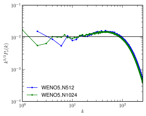
In Figure 18 we show the compensated velocity spectrum, i.e. $k^{5/3}P_{v}(k)$, at time $t=30$ obtained from the data of the two WENO5 runs. More specifically, the low-resolution spectrum is shifted to larger wavenumbers by a factor two and scaled assuming a $k^{-5/3}$ scaling of the spectrum. The rationale behind this procedure is that we are interested in the (eventual) selfsimilar behaviour of the spectrum and it is therefore useful to consider the low-resolution run as a realisation of the same flow as the high-resolution one, but in a smaller volume. In other words, we interpret the spectrum of the low-resolution run as being computed from a subsample of the data of the high-resolution one [see, e.g. Bodo et al. (2011) for a more detailed discussion of the issue of convergence for direct simulations of turbulent flows].

The plot demonstrates the statistical convergence of the simulation, with the exception of the very low-wavenumber part of the spectrum, where the convergence is probably spoiled by the symmetry. At the same time, the plot also shows that only the high-resolution run seems to be able to cover a sufficiently wide part of the inertial range to give a clear indication of the Kolmogorov $-5/3$ scaling.

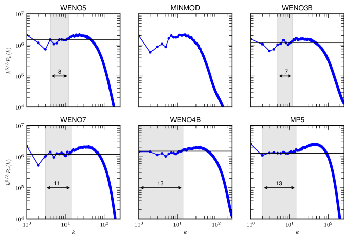
In Figure 19 we show the compensated velocity spectra at time $t=30$ obtained with the different numerical schemes. For each scheme, we highlight with a grey shaded area the part of the spectrum that appears to be “compatible” with the $-5/3$ scaling inferred from the high-resolution WENO5 run. The width of this region, expressed in terms of wavenumbers, is also indicated on the figure. Clearly, this measure has to be taken with a bit of caution, since there is a certain degree of arbitrariness in the identification of the “inertial range”; furthermore, the judgment is also made more difficult by the fact that all of the results are obtained at a resolution which probably is not high-enough and that a convergence study is only available for the WENO5 case. Notwithstanding these caveats, the difference between the various schemes is already sufficiently clear to deduce some of their properties despite the limited amount of data that we were able to generate.

A first conclusion to be drawn is about the importance of the use of high-order schemes, whch is apparent if we compare the different spectra with the one obtained with the MINMOD scheme. This second-order algorithm, in fact, yields a spectrum which is completely dominated by the so-called “bottleneck-effect” [see, e.g. Brandenburg & Nordlund (2011); Schmidt et al. (2006)], i.e. by a region where the power-spectrum shows an excess due to viscous effects. No clear indication of an inertial range appears anywhere in the spectrum, with the only “flat” region being the middle of the bottleneck zone. This could be easily mistaken as the inertial range in the absence of a proper convergence analysis. For this reason, and as remarked many times already, care should be taken while interpreting the results obtained with low-order schemes.

Secondly, we observe that WENO4B has an effective resolution which is about $50\%$ larger then the one from WENO5 and $20\%$ larger then WENO7. Given that saving a factor $1.5$ in resolution corresponds, in 3D to a decrease of the computation costs by a factor five, we conclude that the use of WENO4B over WENO5 is well justified, since WENO4B is roughly twice as expensive as WENO5 in 3D. On the other hand, the spectral resolution of WENO4B does not appear to be better than the one of the MP5 scheme, which has similar computational costs (due to the stricter CFL limitation), but which is also expected to have better parallel scaling because of its more compact stencil. Overall, MP5 shows an “inertial-range” as large as WENO4B. We also note that WENO3B does not seem to yield any improvements over WENO5.

All things considered, the main differences between the bandwidth-optimized schemes and their traditional counterparts seem to lay in the bottleneck region: WENO3B and WENO4B have a much less pronounced bottleneck with respect to WENO5, WENO7 and MP5. This suggests that these schemes should be considered especially for under-resolved turbulent flows, where the spectrum is basically entirely dominated by the dissipation. MP5, on the other hand, can be particularly useful for those problems where one is interested in well-resolved quantities, such as in direct numerical simulations of turbulence, since the scales affected by the numerical dissipation are more easily identified by the pronounced bottleneck. MP5 should also be the scheme of choice in Newtonian hydrodynamics, since there its timestep constraint seems to be less severe.

5 Conclusions

We have presented THC, a new multi-dimensional, finite-difference, high-resolution shock-capturing code for classical and special-relativistic hydrodynamics. THC employs up to seventh-order accurate reconstruction of the fluxes in local characteristic variables and the Roe flux-vector-splitting algorithm with a novel entropy-fix prescription. The multi-dimensional case is treated in a dimensionally unsplit fashion and the time integration is done with a third-order strongly-stability-preserving Runge-Kutta scheme.

We have carried out a systematic comparison of the results obtained with our code using five different reconstruction operators: the classical WENO5, WENO7, MP5, as well as two specialised bandwidth-optimized WENO schemes: WENO3B and WENO4B. For all schemes, we have checked their ability to sharply capture grid-aligned, diagonal or spherical shock waves, and have carried out a rigorous assessment of their accuracy in the case of smooth solutions. Finally, we have contrasted the performance of the different methods in the resolution of small scale structures in turbulent flows. To the best of our knowledge, this is the first time that such a comparison has been carried over in the special-relativistic case.

Among the different tests studied, some are highly nontrivial, such those involving the linear and the nonlinear phases of the development of the Kelvin-Helmholtz instability for a relativistic fluid in two and three dimensions. In particular, we have shown the importance of using schemes that are able to properly capture the initial contact discontinuity in order to obtain the correct growth rate of the RMS transverse velocity in the linear-growth phase of the instability at low resolution, confirming the findings by Mignone et al. (2009) and Beckwith & Stone (2011).

When studying Kelvin-Helmholtz instability in two dimensions, we have investigated the nature of the secondary vortices that appear during the initial stages of the instability when using some of the numerical schemes considered. We have then clarified that these vortices are not genuine features of the solution of the equations, but rather numerical artefacts that converge away with resolution. When studying Kelvin-Helmholtz instability in three dimensions, we have instead investigated the “mixing timescale” of the instability and the subsequent turbulent flow, showing that we are able to obtain a converged measure of the velocity power spectrum, using the WENO5 scheme. Our data offers a clear indication that the Kolmogorov phenomenology (Kolmogorov 1991) holds also for the turbulence in a subsonic relativistically-warm fluid. Using the Kolmogorov $-5/3$ scaling as a reference, we have estimated the effective inertial range of the different schemes, highlighting the importance of using high-order schemes to study turbulent flows. The code has also been used in a systematic investigation of direct numerical simulations of driven turbulence in an ultrarelativistic hot plasma, whose results will be presented in a companion paper (Radice & Rezzolla in prep.).

Finally, THC represents the first step towards the implementation of new and high-order methods for the accurate study of general-relativistic problems, such as the inspiral and merger of binary neutron stars (Baiotti et al. 2011) and their relation with gamma-ray bursts (Rezzolla et al. 2011). We are in fact convinced that the transition towards higher-order methods is now a necessary and an inevitable step for a more realistic description of the complex phenomenology associated with these relativistic-astrophysics processes.

Appendix A Secondary vortices in the KHI

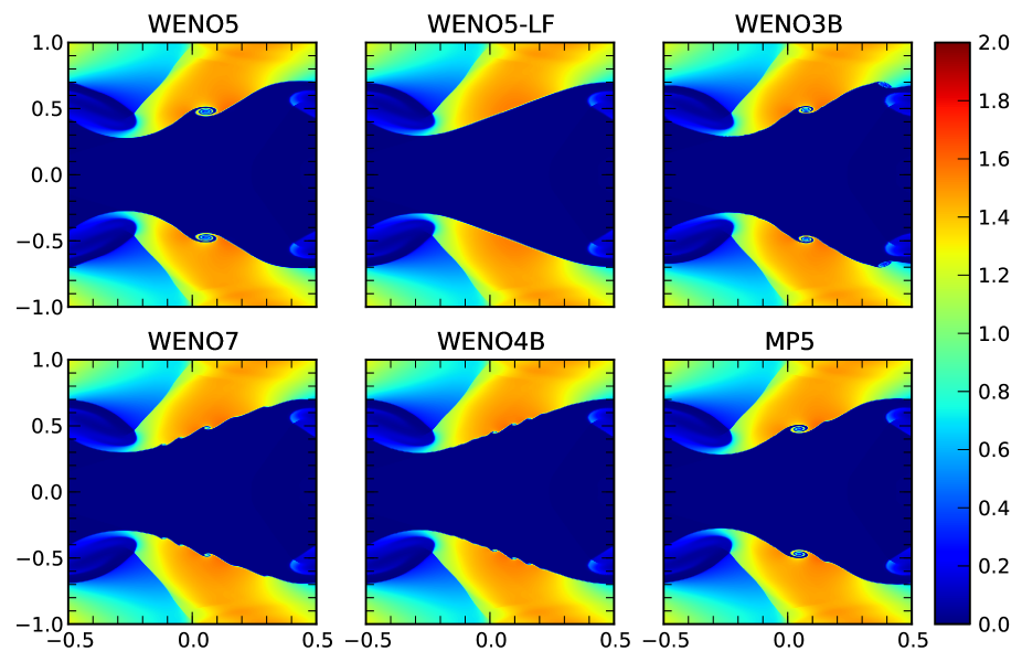
In Sect. 3.2.6 we have commented that we believe the secondary instabilities appearing the in initial stages of the KHI are not genuine features of the solution, but just artefacts of the (low) resolution. The latter acts differently on different schemes, leading to a non-predictable change in the number and shape of these secondary vortices. Convincing evidence that these are indeed artifacts is shown in Figure 20, which is the same as Figure 13, but at the higher resolution of $1024\times 2048$. When comparing the two figures it appears clear that these secondary instabilities are much smaller. Interestingly, therefore, the more dissipative scheme WENO5 with the Lax-Friedrichs flux-split, WENO5-LF, seems to converge more rapidly to the correct solution (at least in these initial stages) than its less diffusive counterparts.

Figure 20: Rest-mass density for the 2D relativistic Kelvin-Helmholtz instability test at time $t=3$ and for different numerical schemes. The resolution is $1024\times 2048$ for all the schemes and the CFL factor is $C\approx 0.25$. This figure should be compared with its equivalent Figure 13 at a resolution $512\times 1024$

References

- Agertz et al. (2007) Agertz, O., Moore, B., Stadel, J., et al. 2007, Monthly Notices of the Royal Astronomical Society, 380, 963
- Aloy et al. (1999) Aloy, M. A., Pons, J. A., & Ibáñez, J. M. 1999, Comput. Phys. Commun., 120, 115
- Aloy & Rezzolla (2006) Aloy, M. A. & Rezzolla, L. 2006, Astrophys. J., 640, L115
- Anile (1990) Anile, A. M. 1990, Relativistic Fluids and Magneto-fluids (Cambridge University Press)
- Antón et al. (2006) Antón, L., Zanotti, O., Miralles, J. A., et al. 2006, Astrophys. J., 637, 296
- Baiotti et al. (2010) Baiotti, L., Damour, T., Giacomazzo, B., Nagar, A., & Rezzolla, L. 2010, Phys. Rev. Lett., 105, 261101
- Baiotti et al. (2011) Baiotti, L., Damour, T., Giacomazzo, B., Nagar, A., & Rezzolla, L. 2011, Phys. Rev. D, 84, 024017
- Baiotti et al. (2008) Baiotti, L., Giacomazzo, B., & Rezzolla, L. 2008, Phys. Rev. D, 78, 084033
- Baiotti et al. (2009) Baiotti, L., Giacomazzo, B., & Rezzolla, L. 2009, Classical Quantum Gravity, 26, 114005
- Baiotti et al. (2003) Baiotti, L., Hawke, I., Montero, P., & Rezzolla, L. 2003, in Computational Astrophysics in Italy: Methods and Tools, ed. R. Capuzzo-Dolcetta, Vol. 1 (Trieste: MSAIt), 210
- Baiotti et al. (2005) Baiotti, L., Hawke, I., Montero, P. J., et al. 2005, Phys. Rev. D, 71, 024035
- Banyuls et al. (1997) Banyuls, F., Font, J. A., Ibáñez, J. M., Martí, J. M., & Miralles, J. A. 1997, Astrophys. J., 476, 221
- Beckwith & Stone (2011) Beckwith, K. & Stone, J. M. 2011, The Astrophysical Journal Supplement Series, 193, 6
- Bernuzzi et al. (2012a) Bernuzzi, S., Nagar, A., Thierfelder, M., & Bruegmann, B. 2012a, arXiv:1205.3403, 12
- Bernuzzi et al. (2012b) Bernuzzi, S., Thierfelder, M., & Brügmann, B. 2012b, Physical Review D, 85
- Bodo et al. (2011) Bodo, G., Cattaneo, F., Ferrari, A., Mignone, A., & Rossi, P. 2011, The Astrophysical Journal, 739, 82
- Bodo et al. (2004) Bodo, G., Mignone, a., & Rosner, R. 2004, Phys. Rev. E, 70, 1
- Brandenburg & Nordlund (2011) Brandenburg, A. & Nordlund, A. k. 2011, Reports on Progress in Physics, 74, 046901
- Chiu (1973) Chiu, H. H. 1973, Physics of Fluids, 16, 825
- Colella & Woodward (1984) Colella, P. & Woodward, P. R. 1984, Journal of Computational Physics, 54, 174
- Del Zanna et al. (2003) Del Zanna, L., Bucciantini, N., & Londrillo, P. 2003, Astron. Astrophys., 400, 397
- Del Zanna et al. (2007) Del Zanna, L., Zanotti, O., Bucciantini, N., & Londrillo, P. 2007, Astron. Astrophys., 473, 11
- Donat et al. (1998) Donat, R., Font, J. A., Ibáñez, J. M., & Marquina, A. 1998, J. Comput. Phys., 146, 58
- Duez et al. (2005) Duez, M. D., Liu, Y. T., Shapiro, S. L., & Stephens, B. C. 2005, Phys. Rev. D, 72, 024028, astro-ph/0503420
- Duffell & MacFadyen (2011) Duffell, P. C. & MacFadyen, A. I. 2011, The Astrophysical Journal Supplement Series, 197, 15
- Dumbser & Zanotti (2009) Dumbser, M. & Zanotti, O. 2009, Journal of Computational Physics, 228, 6991
- Eswaran & Pope (1988) Eswaran, V. & Pope, S. 1988, Computers & Fluids, 16, 257
- Farris et al. (2008) Farris, B. D., Li, T. K., Liu, Y. T., & Shapiro, S. L. 2008, Phys. Rev. D, 78, 024023
- Font (2008) Font, J. A. 2008, Living Rev. Relativ., 6, 4
- Gammie et al. (2003) Gammie, C. F., McKinney, J. C., & Tóth, G. 2003, Astrophys. J., 589, 458
- Giacomazzo & Rezzolla (2007) Giacomazzo, B. & Rezzolla, L. 2007, Classical Quantum Gravity, 24, S235
- Giacomazzo et al. (2009) Giacomazzo, B., Rezzolla, L., & Baiotti, L. 2009, Mon. Not. R. Astron. Soc., 399, L164
- Goodale et al. (2003) Goodale, T., Allen, G., Lanfermann, G., et al. 2003, in Vector and Parallel Processing – VECPAR’2002, 5th International Conference, Lecture Notes in Computer Science (Berlin: Springer)
- Gottlieb et al. (2009) Gottlieb, S., Ketcheson, D., & Shu, C.-W. 2009, Journal of Scientific Computing, 38, 251, 10.1007/s10915-008-9239-z
- Gourgoulhon (1991) Gourgoulhon, E. 1991, Astronomy and Astrophysics, 252, 651
- Inoue et al. (2011) Inoue, T., Asano, K., & Ioka, K. 2011, Astrophys. J., 734, 77
- Jiang & Shu (1996) Jiang, G.-S. & Shu, C.-W. 1996, J. Comput. Phys, 126, 202
- Johnsen et al. (2010) Johnsen, E., Larsson, J., Bhagatwala, A. V., et al. 2010, Journal of Computational Physics, 229, 1213
- Kastaun (2006) Kastaun, W. 2006, Phys. Rev. D, 74, 124024
- Kastaun (2007) Kastaun, W. 2007, PhD thesis, University of Tübingen
- Kitsionas et al. (2009) Kitsionas, S., Federrath, C., Klessen, R. S., et al. 2009, Astronomy and Astrophysics, 508, 541
- Koide et al. (1999) Koide, S., Shibata, K., & Kudoh, T. 1999, Astrophys. J., 522, 727
- Kolmogorov (1991) Kolmogorov, A. N. 1991, Proceedings of the Royal Society A: Mathematical, Physical and Engineering Sciences, 434, 9
- Komissarov (2004) Komissarov, S. S. 2004, Mon. Not. R. Astron. Soc., 350, 1431
- Konigl (1980) Konigl, A. 1980, Physics of Fluids, 23, 1083
- Kulikovskii et al. (2001) Kulikovskii, A., Pogorelov, N., & Semenov, A. Y. 2001, Mathematical aspects of numerical solution of hyperbolic systems (Chapman & Hall/CRC)
- Leveque (1992) Leveque, R. J. 1992, Numerical Methods for Conservation Laws (Basel: Birkhauser Verlag)
- Liu et al. (1994) Liu, X.-D., Osher, S., & Chan, T. 1994, Journal of Computational Physics, 115, 200
- Mann (1985) Mann, P. 1985, Journal of Computational Physics, 58, 377
- Martí et al. (1991) Martí, J. M., Ibáñez, J. M., & Miralles, J. A. 1991, Phys. Rev. D, 43, 3794
- Martí & Müller (2003) Martí, J. M. & Müller, E. 2003, Living Rev. Relativ., 6, 7
- Martín et al. (2006) Martín, M. P., Taylor, E. M., Wu, M., & Weirs, V. G. 2006, Journal of Computational Physics, 220, 270
- May & White (1966) May, M. M. & White, R. H. 1966, Phys. Rev., 141, 1232
- McNally et al. (2011) McNally, C. P., Lyra, W., & Passy, J.-c. 2011, arXiv:1111.1764, 24
- Meier (1999) Meier, D. L. 1999, The Astrophysical Journal, 518, 788
- Mignone et al. (2005) Mignone, A., Plewa, T., & Bodo, G. 2005, The Astrophysical Journal Supplement Series, 160, 199
- Mignone et al. (2010) Mignone, A., Tzeferacos, P., & Bodo, G. 2010, Journal of Computational Physics, 229, 5896
- Mignone et al. (2009) Mignone, a., Ugliano, M., & Bodo, G. 2009, Monthly Notices of the Royal Astronomical Society, 393, 1141
- Neilsen et al. (2006) Neilsen, D., Hirschmann, E. W., & Millward, R. S. 2006, Classical Quantum Gravity, 23, S505
- Noh (1987) Noh, W. 1987, Journal of Computational Physics, 72, 78
- Obergaulinger et al. (2010) Obergaulinger, M., Aloy, M. A., & Müller, E. 2010, Astronomy and Astrophysics, 515, A30
- Perucho et al. (2007) Perucho, M., Hanasz, M., Martí, J.-M., & Miralles, J.-A. 2007, Phys. Rev. E, 75, 1
- Perucho et al. (2010) Perucho, M., Martí, J. M., Cela, J. M., et al. 2010, Astronomy and Astrophysics, 519, A41
- Plewa & Mueller (1999) Plewa, T. & Mueller, E. 1999, Astronomy and Astrophysics Astrophysics, 342, 179
- Pons et al. (2000) Pons, J. A., Martí, J. M., & Müller, E. 2000, J. Fluid Mech., 422, 125
- Porter et al. (2002) Porter, D., Pouquet, A., & Woodward, P. 2002, Phys. Rev. E, 66, 1
- Quirk (1994) Quirk, J. 1994, International Journal for Numerical Methods in Fluids, 18, 555
- Radice & Rezzolla (2011) Radice, D. & Rezzolla, L. 2011, Phys. Rev. D, 84, 024010
- Rezzolla et al. (2011) Rezzolla, L., Giacomazzo, B., Baiotti, L., et al. 2011, Astrophys. J., 732, L6
- Rezzolla & Zanotti (2002) Rezzolla, L. & Zanotti, O. 2002, Phys. Rev. Lett., 89, 114501
- Rezzolla et al. (2003) Rezzolla, L., Zanotti, O., & Pons, J. A. 2003, Journ. of Fluid Mech., 479, 199
- Rider (2000) Rider, W. 2000, Journal of Computational Physics, 162, 395
- Roe (1981) Roe, P. L. 1981, J. Comput. Phys., 43, 357
- Rosswog (2010) Rosswog, S. 2010, Journal of Computational Physics, 229, 8591
- Schmidt et al. (2006) Schmidt, W., Hillebrandt, W., & Niemeyer, J. 2006, Computers & Fluids, 35, 353
- Schneider et al. (1993) Schneider, V., Katscher, U., Rischke, D. H., et al. 1993, J. Comput. Phys., 105, 92
- Sekiguchi (2010) Sekiguchi, Y. 2010, Progress of Theoretical Physics, 124, 331
- Sekiguchi et al. (2011) Sekiguchi, Y., Kiuchi, K., Kyutoku, K., & Shibata, M. 2011, Phys. Rev. Lett., 107, 051102
- Shu (2007) Shu, C. 2007, Lecture Notes Series, Institute for Mathematical Sciences, National University of Singapore, 11, 47
- Shu (1997) Shu, C. W. 1997, Essentially non-oscillatory and weighted essentially non-oscillatory schemes for hyperbolic conservation laws, Lecture notes ICASE Report 97-65; NASA CR-97-206253, NASA Langley Research Center, http://techreports.larc.nasa.gov/icase/1997/icase-1997-65.pdf
- Shu (1999) Shu, C. W. 1999, in High-Order Methods for Computational Physics, ed. T. J. Barth & H. Deconinck (Springer), 439–582
- Shu (2001) Shu, C. W. 2001, High order finite difference and finite volume WENO schemes and discontinuous Galerkin methods for CFD, Tech. Rep. ICASE Report 2001-11; NASA CR-2001-210865, NASA Langley Research Center
- Shu & Osher (1988) Shu, C. W. & Osher, S. J. 1988, J. Comput. Phys., 77, 439
- Siegler & Riffert (2000) Siegler, S. & Riffert, H. 2000, The Astrophysical Journal, 531, 1053
- Sod (1978) Sod, G. A. 1978, Journal of Computational Physics, 27, 1
- Springel (2010) Springel, V. 2010, Monthly Notices of the Royal Astronomical Society, 401, 791
- Suresh & Huynh (1997) Suresh, A. & Huynh, H. T. 1997, Journal of Computational Physics, 136, 83
- Taylor et al. (2007) Taylor, E. M., Wu, M., & Martín, M. P. 2007, Journal of Computational Physics, 223, 384
- Tchekhovskoy et al. (2007) Tchekhovskoy, A., McKinney, J. C., & Narayan, R. 2007, Monthly Notices of the Royal Astronomical Society, 379, 469
- Toro (1999) Toro, E. F. 1999, Riemann Solvers and Numerical Methods for Fluid Dynamics (Springer-Verlag)
- Wilson (1972) Wilson, J. R. 1972, Astrophys. J., 173, 431
- Woodward & Collela (1984) Woodward, P. & Collela, P. 1984, J. Comput. Phys., 54, 115
- Yang (2000) Yang, D. 2000, C++ and Object-Oriented Numeric Computing for Scientists and Engineers (Springer-Verlag)
- Zanotti et al. (2011) Zanotti, O., Roedig, C., Rezzolla, L., & Del Zanna, L. 2011, Mon. Not. R. Astron. Soc., 417, 2899
- Zhang & MacFadyen (2006) Zhang, W. & MacFadyen, A. 2006, The Astrophysical Journal Supplement Series, 164, 255
- Zhang et al. (2009) Zhang, W., MacFadyen, A., & Wang, P. 2009, Astrophys. J., 692, L40
- Zrake & MacFadyen (2012) Zrake, J. & MacFadyen, A. I. 2012, Astrophys. J., 744, 32