Notes on the integration of numerical relativity waveforms
Abstract
A primary goal of numerical relativity is to provide estimates of the wave strain, , from strong gravitational wave sources, to be used in detector templates. The simulations, however, typically measure waves in terms of the Weyl curvature component, . Assuming Bondi gauge, transforming to the strain reduces to integration of twice in time. Integrations performed in either the time or frequency domain, however, lead to secular non-linear drifts in the resulting strain . These non-linear drifts are not explained by the two unknown integration constants which can at most result in linear drifts. We identify a number of fundamental difficulties which can arise from integrating finite length, discretely sampled and noisy data streams. These issues are an artifact of post-processing data. They are independent of the characteristics of the original simulation, such as gauge or numerical method used. We suggest, however, a simple procedure for integrating numerical waveforms in the frequency domain, which is effective at strongly reducing spurious secular non-linear drifts in the resulting strain.
pacs:
04.25.dg, 04.30.Db, 04.30.Tv, 04.30.Nk1 Introduction
With the advent of gravitational wave detector experiments, the concept of metric strain has been elevated from a theoretical result of the linearized Einstein equations, to a genuine physical observable which will be directly measured for the first time in the coming years. Since they are weak, foreknowledge of the expected signals will greatly aid the initial detection and subsequent understanding of measurements. Thus, a number of major efforts are going into constructing high-precision models of dynamical spacetimes, in order to determine what the detectors will see from strongly radiating burst sources such as binary black hole and neutron star mergers.
Numerical models have achieved some timely successes in recent years [1, 2, 3], so that the final orbits, merger and ringdown of binary black holes can be modeled with high numerical accuracy. Templates for these waveforms are being constructed by matching the numerical results to post-Newtonian inspirals, for instance using the effective one-body approach [4, 5, 6, 7, 8], or purely phenomenological models [9, 10, 11, 12]. Meanwhile, these models are already being tested in detector search pipelines [13, 14, 15].
In constructing templates, the natural observable is the one which is also measured by the detectors, namely the gravitational wave strain , decomposed into ‘’ and ‘’ polarizations in the transverse-traceless gauge. However, this is typically not the quantity which is directly computed in numerical simulations, where the output of numerical simulations is more usually in the form of curvature tensor components, or Zerilli-Moncrief-type variables defined relative to a background. The results are then transformed to determine the standard and strain modes in order to connect to the detector measurements.
Transforming the measured variables to the strain involves some numerical subtleties. In particular, it has long been noted that producing a strain, , from the Newman-Penrose curvature component, , typically results in a waveform with an unphysical secular non-linear drift (e.g. [16, 17]). The fact that this drift is non-linear indicates that it is not simply a result of the two unknown integration constants involved in the transformation. A potential source of the problem may come from the fact that is typically extracted at a finite distance from the gravitating source ([18] and references therein). The strain , however, is related to only at an infinite distance from the source hence introducing a systematic “finite-radius” error. Furthermore, the relation between and is strictly only valid in a particular gauge. This gauge, however, is typically not imposed during the simulations but is given by the the gauge driver controlling the gauge during the evolution ([18] and references therein), and may thus also lead to secular effects like the observed non-linear drift in the strain. By eliminating these systematic errors, one would therefore hope to greatly reduce the secular behavior. Unfortunately, even with the recent possibility of extracting truly gauge-invariant waveforms at future null infinity [19, 20], we still observe non-linear contributions to the drifts on time integration of the results, even though the measurement is free of gauge and finite-radius errors. This suggests that the source of the problem must have different roots.
This paper argues that an important source of unphysical non-linear drift in numerical computations of gravitational wave strain lies in the transformation of the measured data (commonly the Newman-Penrose variable ) to the observable strain , which generically involves an integration in time. The output of the numerical simulation is a discretely sampled time series of finite duration, incorporating some component of unresolved frequencies due to numerical error. The latter aspect can lead to an uncontrollable non-linear drift if the integration is performed in the time domain. An alternative is to perform the integration in the frequency domain (e.g., [21, 12]). In this case, however, the finite duration of the numerical signal becomes an issue, as artificial low-frequency components of the infinite spectrum of a localized-in-time function dominate the integral. An appropriately chosen band-pass filter improves the situation greatly. Unfortunately, this can require some complicated adjustment of parameters, which is difficult to systematize.
We first outline some numerical problems inherent in determining the strain from gauge-invariant quantities typically used in spacetime simulations, discussing aspects of time and frequency domain integrations, and the use of band filters. Finally we arrive at a new and constructive procedure for performing the required numerical integrations, fixed frequency integration (FFI), which involves a single parameter related to the lowest physical frequency component of the wave. The method is effective at reducing secular non-linear drifts in , while maintaining the energy of the wave. We demonstrate our results with numerically generated gravitational waveforms, as well as with some artificial analytic functions in order to gauge the potential errors.
2 Evaluating gravitational strain from numerical data
Gravitational waves are dynamic solutions of the nonlinear Einstein equations, which are most readily described by perturbations of a fixed background metric:
| (1) |
where is a fixed background, and is a perturbation containing the wave. The observables measured by a gravitational wave detector are the strain components, and , in the transverse-traceless (TT) gauge. A number of techniques are available for computing these variables, though usually dependent on some underlying assumptions regarding the spacetime within a simulation, and coordinates at some finite distance from the source.
One practical method for evaluating gravitational waves is based on the extensive work that has been done defining perturbative variables that are gauge invariant relative to a fixed spherical or axisymmetric background. Early perturbative studies of black hole spacetimes [22, 23, 24] formalized a 1st-order gauge invariant representation of the variables. These methods have been applied to numerical relativity simulations for some years [25, 26, 27] (see [28] for recent comparisons with -based measurement). Briefly, the formalism defines a set of 1st-order even and odd-parity gauge invariant variables, , describing the metric perturbation. The and components of the strain in the TT-gauge are determined via:
| (2) |
where is the distance to the source, the observation time, and are spin-2 spherical harmonics.
Alternatively, the curvature can be expressed in terms of Newman-Penrose (NP) components in a given null frame [29]. Ideally, this is performed at null infinity, , where the frame and coordinates can be invariantly specified, and the fall-off of the curvature is known for asymptotically flat spacetimes. Procedures for invariant measures at have recently been developed as a practical tool [19, 20]. However, at a large but finite distance from the source, accurate measurements can also be made simply by evaluating the curvature relative to a radially oriented null frame. The gravitational wave information is determined either from the asymptotically defined Bondi news [30, 31] 111See also [32] for a recent discussion in the context of 3+1 numerical relativity.,
| (3) |
(in the NP notation) or the Weyl curvature component . Then the strain is determined by:
| (4) |
Significantly, for any of these choices of gauge invariant observable, , or , we only recover the strain, , after one or multiple integrations in time. One time integral is required in the case of the perturbative techniques and the Bondi news, , (as well as the strain-rate, , defined in [33]), while two are required to calculate from . In practice, the integration is not performed from , but starts at a particular point, the beginning of the simulation. This introduces one or two integration constants in Eq. (2) and Eq. (4), respectively. The integrated result therefore yields at most a linear drift, which can easily be removed by fixing the integration constants, e.g. by an averaging procedure.
In practice, numerical integration of a time series can be performed through standard methods, for instance, a simple application of Simpson’s rule. However, in the case of gravitational waveform data, after having fixed the integration constants to remove the linear drift, these procedures tend to introduce a residual non-linear drift which is, at best, a significant nuisance to analysis, but may also be confused with physical modes in which secular drifts are expected [16, 17]. An example of the problem is shown in Fig. 1, which plots the spherical harmonic mode of the strain, , determined by integrating a numerical over the last cycles of a non-spinning () equal-mass () binary black hole merger [34, 35]. We plot the results of time integrations via an extended 4th-order Simpson’s rule, by an Adams-Moulton integration, as well as a 2nd-order midpoint rule [36]. We have choosen the first integration constant such that the signal is zero after ringdown. The second integration constant was set to zero. Whereas we expect the result to oscillate about zero, in fact we observe a prominent non-linear drift, which is independent of the numerical integration method. Similar artifacts have been observed in waveform computations from different simulations, for instance early ringdown results [16], as well as more recent studies [17, 37].
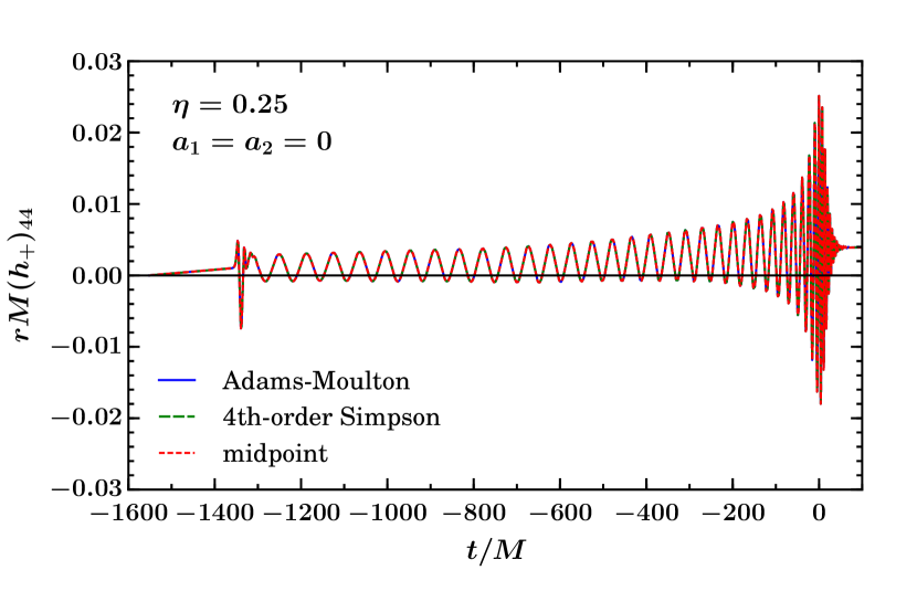
One can imagine a number of systematic sources for the unphysical non-linearities of the drift, resulting from the way measurements are made within the simulation. For measurements at finite radius, the observer location (typically a sphere at some radius defined by grid coordinates) changes over time for the dynamical coordinate conditions which are in common use. However, the waveforms plotted in Fig. 1 are measured at , via characteristic extraction [19, 20]. As such, they should be immune to local coordinate effects, and indeed, examination of using different worldtube data and different resolutions reveal that the differences in converge to zero [19, 20]. This suggests that the source of the problem must have different roots. One potential source of error is given by the time integration itself, as we discuss below.
3 Numerical integration of time-series data
The waveforms generated by numerical relativity simulations are discretely sampled time-domain representations of a finite-length signal possibly contaminated by numerical “noise”. The problems arising from integrating discretely sampled numerical (or, especially, experimental) data, and are well known in other fields of physics and engineering [38]. A clear analogy comes from the use of accelerometer data to determine a position. While the source of the problems are easy to identify, unfortunately a rigorous solution, particularly without a detailed characterization of the experimental noise, is difficult for time-domain integrations.
3.1 Time-domain integration
Consider an integral of the form
| (5) |
If is known exactly, then we can evaluate the integral numerically according to a standard scheme, and the integral will converge to its continuum representation in the limit of infinite resolution. However, if the function contains small amounts of experimental (or numerical) noise, this has a significant impact on the accuracy of the time integration as we will see below.
To motivate the aspect of numerical noise, consider a convergent finite differencing code yielding a truncation error which can be modeled by a continuous polynomial, :
| (6) |
where is exact and its numerical approximation. Then, the integration yields
| (7) |
provided that itself is sufficiently resolved.
In numerical relativity data, however, the convergence exponent of the measured waveforms is commonly of an order which is higher than the lowest order of the underlying finite differences used to generate the result, such as the time-interpolation at mesh-refinement boundaries, or the Runge-Kutta time integrator. That is, the results are superconvergent. This may come about if the error coefficient of the low order operations is too small to be measured, or may also be associated with under-resolution of some features of the model. Further, the measured convergence exponents are often non-integer values, not corresponding to the order of any discrete operation of the code, and may vary in time, particularly during the late stages of an inspiral simulation. The error polynomial of the one-dimensional time series waveform is the combination of the error polynomials of a number of independent discrete operations, including finite-differencing, interpolation, and reduction. If any of these intermediate operations under-resolves the cumulative error (for example, if the end product is down-sampled), the result will be a contribution to the signal which though deterministic, mimics the character of numerical noise. We illustrate the effect in an analytic example.
High-frequency components of the waveforms (whether truly random noise, a deterministic effect of discrete operators, or actual physical modes) are aliased onto the low-frequency physical signal. This can have a profound effect on operations such as integration. To demonstrate this, we model the numerical estimate of some exact function by
| (8) |
where is the exact result, and is a continuous function representing the truncation error of , sampled at discrete points .
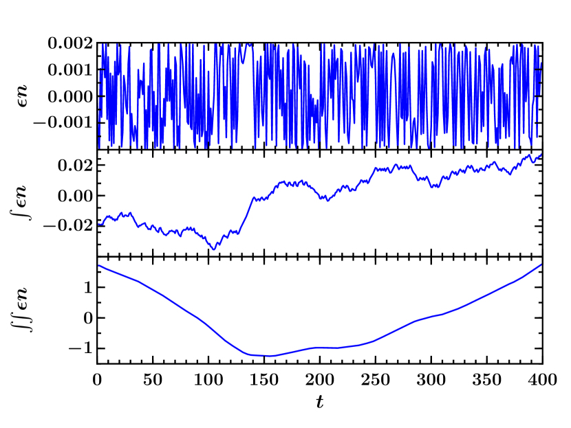
We illustrate the effect of aliasing on integration in Fig. 2. We have integrated a signal which is composed purely of truncation error (i.e. ), modeled by a sinusoid,
| (9) |
whose frequency varies in time between the values and , according to Eq. (31), below. The upper panel plots the original data, sampled at an interval of . The function oscillates near the Nyquist frequency, and is clearly under-resolved. Its first and second integrals (in the middle and lower panels of Fig. 2, respectively) are analagous to what would be expected from a random-walk. In that case, the integral over the data points does not avarage out for large . Rather, the size of the drift, i.e., the root mean squared expected translation distance after steps, is given by the standard deviation of the imposed probability distribution and will grow without bounds with the total number of steps (see e.g., [39]).
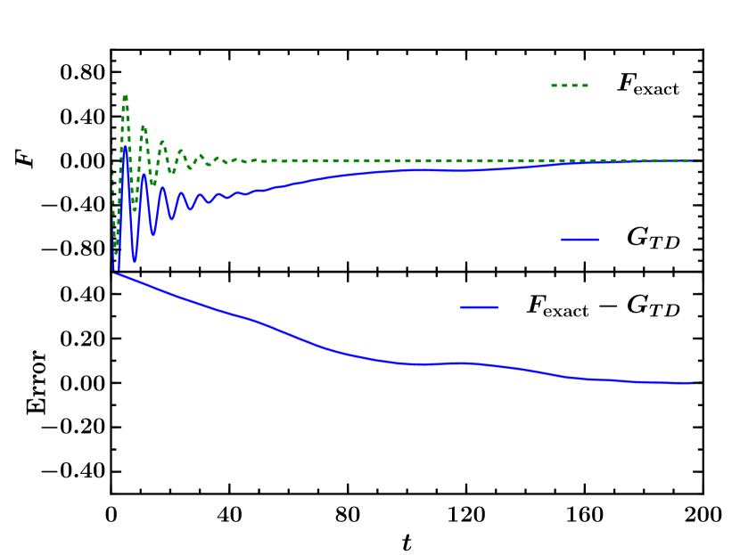
In Fig. 3, we show the effect of an under-resolved low-amplitude, high-frequency component on the integration of a damped oscillatory function reminiscent of a black hole ringdown,
| (10) |
for which we choose and damping parameter . We fix the frequency at and evaluate the function on the interval , at discrete points with uniform spacing . We directly integrate numerically using a variant of Simpson’s rule (see [36], for example, though as suggested in Fig. 1, the results are largely independent of the particular method) to compute
| (11) |
Since the model is analytically defined, the error in the evaluation at each point is given by machine double-precision (, or approximately ), and the numerical integration reproduces the exact result with high accuracy.
Consider now the effect of a small high-frequency error component which we will again model by Eq. (9), with an amplitude , and frequency parameters , , and . The resulting numerical double integration , together with the analytically known double time integral of (10) is plotted in Fig. 3. A non-linear drift, four orders of magnitude larger than the originally induced error, is apparent in the integral of the modified waveform.
3.2 Frequency-domain integration of finite-length signals
An alternative method for numerical integration of a time series arises from simply transforming the problem to the frequency domain. Consider the Fourier transform, , applied to an absolutely integrable function ,
| (12) |
The Fourier transform of the time integral of is given by
| (13) |
and we arrive at a simple expression for the time-domain representation of the integral of in terms of the inverse Fourier transform:
| (14) |
In the frequency-domain, time integration becomes a simple division by the frequency. Thus, the method is particularly susceptible to low-frequency error. For instance, under-resolved high-frequency modes can be aliased onto low-frequency modes of the signal.
More important is the fact that any numerically generated (or experimentally measured) time series is necessarily finite in length. For frequency-domain methods, the localization of the signal in time poses a fundamental difficulty, arising from the properties of the Fourier transform. The observation of any finite duration signal is equivalent of multiplying an infinite signal with a rectangular window function. According to the convolution theorem, multiplying a signal with another signal in the time domain corresponds to convolving the Fourier transformed signals in the frequency domain. Because the frequency representation of the rectangular window function is the function, which has infinite bandwidth, the same is true of the convolved signal.
This phenomenon, sometimes termed spectral leakage, can be demonstrated through a simple example. Trivially, the Fourier transform of a function of infinite extent with constant oscillation frequency, ,
| (15) |
is a Dirac delta function centred at . However, a wave of finite duration, can not reduce to a Dirac delta function in the frequency domain due to spectral leakage. Rather, the spectrum will have a peak at , but other frequencies, particularly those close to , will have non-zero values. It is worthwhile to emphasize that this is not an artifact of the discrete Fourier transform. It is an artifact of the finite time duration of the signal.
The problem of spectral leakage has important consequences for time integration in the frequency domain, particularly due to the division by at the low-frequency end of the spectrum. Consider the time integral of Eq. (15) in the frequency domain, which is trivially given by
| (16) |
If the same function is truncated in the time domain (i.e. windowed by the rectangular window function to some finite interval ), the resulting Fourier spectrum is still peaked at , but will be non-zero over an extended range. The original delta function is “smeared out”, and will affect the time integral
| (17) |
where denotes the frequency distribution of the windowed function arising from spectral leakage. Division by the frequency results in amplification of low-frequency components of other than , and is responsible for secular drifts when the time-domain signal is reconstructed.
The distribution, , can be modified by altering the implicit rectangular window function associated with the finite-length signal by tapering or fading towards the edges of the time domain [40, 41]. However, there are well-documented trade-offs, and the phenomenon of spectral leakage can never be entirely compensated.
We note that for the particular case of the analytical example, Eq. (15), the genuine oscillation frequency is known. By dividing only by in the function on the right-hand side of Eq. (17), we find that we recover in the time domain a result which is the exact time intergal with the integration constants set such that the signal is oscillating about zero.
In the case of gravitational waveforms, we do not have a fixed frequency. However for the most interesting physical models, such as late-time binary inspiral, the range of relevant frequencies is approximately set by the initial orbital timescale and the ringdown frequency. We will show in Section 4.2 that exploiting this knowledge leads to an effective and simple integration scheme which greatly reduces the impact of spectral leakage, very similar to the simple example Eq. (15).
4 Optimized filters and improved frequency-domain integrations
The effect of the spurious low-frequency modes, resulting from either spectral leakage or aliasing effects, can be significantly suppressed through the use of signal filters. In particular, a high-pass filter can be used to reduce the energy contained in frequencies lower than a chosen cutoff. As noted in [12], an appropriate choice of filter which suppresses modes of frequency lower than the initial instantaneous frequency of the waves, significantly improves the form of the integral.
4.1 High-pass filters and window functions
An ideal filter is the simple step function, or a brick-wall filter, which sets everything below the cut-off frequency to zero while passing (leaving unchanged) the higher frequency components. This filter method has previously been used in [21] (see also [13]) in the context of numerical relativity waveform integration. In practice, however, this filter can be problematic as it gives rise to Gibbs phenomena on transformation to the time domain. To suppress these effects, it is therefore preferable to introduce a smooth transition region between the stop and pass band. The particular choice of the transition function is delicate, as the wrong fall-off can result in significant oscillations in the amplitude of the reconstructed time-domain signal.
The tapering function (or window) is effectively the transfer function, , defined by
| (18) |
where is the original signal, and the filtered signal. Applying a window function is equivalent to imposing a certain function to in order to arrive at the filtered signal from the original data.
Santamaria et al. [12] apply a window of the form:
| (19) |
where the parameters , must be chosen. Meanwhile, McKechan et al. [42] have analyzed the properties of a tapering window in the time domain based on a Planck-distribution, in order to minimize oscillations in the frequency domain. In practice, applying a transfer function such as Eq. (19) in the frequency domain requires some non-trivial fine-tuning as there are two free parameters, and , which have a sensitive effect on the removal of non-linear drifts in the reconstructed time-domain signal. In addition, the choice of window parameters are not easily generalizable to different simulation models and the various other (higher) harmonic modes as each mode requires an indiviudal and different set of fine-tuned parameters.
To circumvent these problems, we propose a different ansatz. Instead of imposing a particular transfer function through the choice of a fixed window function, we derive an appropriate transfer function, , from the data in order to reduce the amount of required fine-tuning significantly. Our proposal is guided by the following observation. By setting the power spectrum to
| (20) |
for frequencies below a chosen frequency , we find that we can minimize non-linear drifts arising in the time domain by an appropriate choice of the parameters and , and this behavior is generic for different (higher) harmonic modes. This frequency fall-off is similar to that of a Butterworth filter [43, 40], known to result in a maximally flat response in the frequencies that are passed. The empirically observed result of applying such a filter is to suppress non-linear drifts of the centre of the waves away from zero, which is the source of ripples in the amplitude. The drawback is a slower roll-off towards low frequencies, which means that part of the signal at low frequencies will be lost due to the transition.
Specifically, we can carry out integrations as follows. First, we transform individual oscillating spherical harmonic modes of to the frequency domain. In a - plot, functions of the form Eq. (20) are linear, with slope . Empirically, we find that we can remove the drifts in the time domain by setting the power spectrum to
| (21) |
where the coefficients and are determined by fitting to a section of the waveform over a chosen interval , which is below the lowest instantaneous physical frequency of the model, and where the spectrum is approximately linear in the - plot. We compute
| (22) |
(where ‘’ indicates the complex modulus). From this we determine
| (23) |
In order to control the power spectrum below , we compute the transfer function according to
| (24) |
and use pointwise multiplication to determine
| (25) |
We can then determine as the 2nd time integral of , according to Eqs.(4) and (14),
| (26) |
and apply the inverse Fourier transform to obtain the result in the time domain. With a careful choice of a frequency fitting interval, we find that the resulting strain, , is free of non-linear drifts and spurious oscillations. An example is plotted in Figs. 5 and 5. Once an optimal set of parameters , has been found, the same procedure can be applied to higher harmonic modes without additional fine-tuning by using the relation , which is a result of the phase relation of the spherical harmonics .
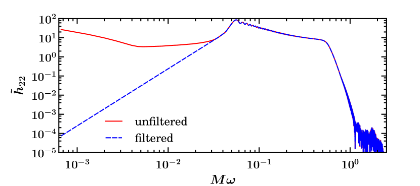
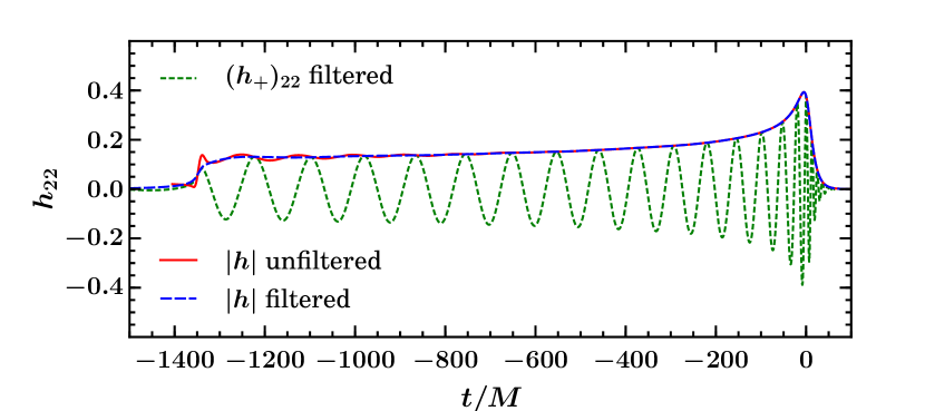
Although the filtering technique is effective in limiting non-linear drift artifacts of the reconstructed time-domain signal, a principle drawback is the assumption that the power spectrum of the transformed signal contains a segment below which allows for a linear fit in the log-log function plot. While empirically this is the case for binary black hole waveforms, we find that more general waveforms such as signals from stellar core collapse signals (see e.g., [44]) do not have such simple power spectra, making the choice of falloff exponent, , more difficult.
4.2 Fixed frequency integration (FFI)
A much simpler, yet empirically more robust, method for integrating in the frequency domain is suggested by the simple example discussed in Sec. 3.2. For the analytically known function with a single frequency component, the integration is greatly improved (in the sense of removing spurious non-linear drifts) by applying information about the expected frequency band to control the amplification of the unphysical frequencies resulting from spectral leakage. That example involves only a single oscillation frequency, , and by simply multiplying with it is possible to achieve drift-free integration.
However, an astrophysically interesting waveform such as that of a binary black hole merger is characterized by a range of physical frequencies, primarily determined by the intial orbital velocity and increasing to the ringdown frequency, for each mode, so that the true physical frequency content is approximately222We note that the true physical frequency range is slightly larger. For instance, the exponentially damped ring-down signal is a Lorentz distribution in the Fourier domain, even though it contains a single QNM oscillation frequency. For exponentially damped signals, a more natural way of describing the frequency content is given by the Laplace transform where damped signals with a single (complex) frequency transform to a Dirac delta function. within . In the Fourier transformed wave, any frequencies outside of this band are dominated by the effect of spectral leakage of the finite length time-domain signal.
By effectively applying the same integration method as proposed for the example Eq. (15) to the range of physically relevant frequencies, , we find that the spurious non-linear drifts due to the amplification of unphysical (spectrally-leaked) low-frequency modes are essentially removed.
Accordingly, we propose to evaluate the integral using the following prescription:
| (27) |
In order to get the second integral, we simply divide by and , respectively. The single free parameter is , which is set according to the lowest expected physical frequency for the given wave mode. When adjusted correctly, we find that the time-domain representation of the waveform is essentially free of low-frequency drifts. An upper, high-frequency, integration limit via some additional parameter could also be incorporated in Eq. (27), however is not needed for the particular waveforms studied here, given the exponential ringdown, combined with the fact that high frequency errors are not as strongly amplified on integration.
In practice, the choice of requires a certain amount of tuning. A small value will amplify unphysical low-frequency components during the integration process, while a large value may suppress some desired physical frequencies of the waveform. However, the choice is clearly guided by the known features of the original signal, and as will be demonstrated below, improved integrations result from a broad range of the choice of .
The main advantage of the FFI method over windowing functions as described in the previous section is simplicity and generality. By tuning a single parameter, we are able to eliminate the bulk of the linear and non-linear drift in the waveform. This frees the integration from ambiguities in the choice of optimal windowing functions and their respective parameters and can easily be automatized for all higher modes through the relation , once a particular has been found for the dominant mode.
As a final remark, we note that in certain situations, the result of the FFI can be improved by first applying a window function to the time domain signal before transforming to the Fourier domain. This is particularly the case for signals which do not start and end with zero amplitude. In these situation, a window function of the form Eq. (19) may be applied such that the signal smoothly blends from and to zero at beginning and end, respectively. Emperically, we find that the choice of time-window parameters does not require much fine-tuning as long as the transition region is chosen to be sufficiently broad.
4.3 Error estimates for an analytic model
The frequency-domain integration methods avoid the random-walk effects associated with time-domain integration, however they are only able to reduce the problem of spectral leakage at the cost of modifying the original data by introducing spurious low frequencies (via the Fourier transform) which must subsequently be suppressed. A concern is that in the process, physical information may be lost or altered. The magnitude of this effect is difficult to gauge using numerical waveform data for which an exact solution for is not known a priori. We apply the method to an analytic model which exhibits the main features of a binary chirp signal, so that the effects of numerical error and integration methods can be compared against a known result.
We introduce a simple analytic toy-model which provides a rough approximation to some of the properties of a typical inspiral waveform over some cycles, including the merger and ringdown. We construct an artificial strain according to the oscillating function
| (28) |
where
| (29) | |||||
| (30) |
Here, functions have been used to control various transitions between essentially constant values. The amplitude rises from zero at time over a distance , to an amplitude of approximately . The choice of parameters , , , and , control the size, shape and location of an eventual peak in the amplitude. The choice of phase, , leads to a frequency evolution of the form
| (31) |
The frequency transitions from an initial value of approximately for small , to as , over an interval whose location and width are controlled by and , respectively. An example profile for Eq. (28) is shown in the upper panel of Fig. 6, corresponding to the particular parameter choices:
| (32a) | |||||
| (32b) | |||||
| (32c) | |||||
| (32d) | |||||
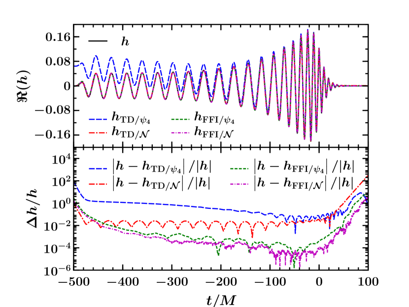
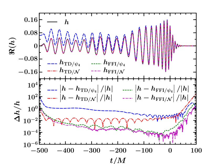
We test the numerical integration methods by determining analytic news, , and curvature component , functions according to
| (32ag) |
These functions are sampled at discrete points, , over an interval, and adjusted by the sinusoidal error function, Eq. 9, to simulate a level of underresolved truncation error in the numerical data:
| (32ah) |
We then reconstruct by performing numerical integrations of Eq. (32ah), and compare the result with the original analytic function, Eq. (28).
Some representative results are plotted in Fig. 6. For this test, we have sampled and at 6000 equally spaced points () over an interval from to , and adjusted the data by an error signal modeled by the underresolved wave Eq. 9 with an amplitude . We compare the strain computed by performing the integrals of and in the time domain (TD, via a 4th-order Simpson’s rule), with those of the FFI method, described in the previous section. For the latter, we note that the starting frequency for the test waveform is , and thus choose a somewhat smaller cutoff frequency for the FFI scheme described by Eq. (27). The results show a prominent drift for the case of two time-domain integrations (). The situation is greatly improved if only a single integration is required (). The lowest level of error results from the FFIs, again with a slight advantage if only a single integration needs to be performed. The results are robust against the particular choice of , and we find that values between 0.02 and 0.2 outperform the time-domain integration at this level of error. Similar levels of error can also be attained by the high-pass filter methods, described in Sec. 4.1, with correctly chosen parameters.
A particular concern with the FFI method (as well as with the use of high-pass filters, as in the previous section) is that any genuine physical low-frequency information will be modified during the integration process. In a binary system, lower frequency components may arise, for instance, due to precession effects, or ellipticity (including zoom-whirl behaviour [45, 46]). We mimic the presence of such features in the toy-model by modulating the amplitude of the analytic wave according to the function
| (32ai) |
where determines the amplitude of the new component, and its frequency. In Fig. 7, we plot the analytic determined by Eq. (28) with replaced by , using the parameters , . We find that since the low-frequency mode has a rather small influence on the Fourier spectrum, the FFI method accurately reproduces the mode in the integrated waveform and continues to outperform time-domain integration. A possible explanation for this behavior might be given by the fact that an amplitude modulation like Eq. (32ai) results in additional effective oscillations (sidebands) of frequency in the signal. Thus, if is small, then the effective contributing lowest frequency is only slightly lower than the initial orbital frequency .
It is difficult to make rigorous quantitative statements about the expected level of error based on these tests, particularly since the analytic waveform is only superficially similar to a genuine inspiral model. Tests with a variety of alternate functions and parameter choices, however, suggest that the qualitative picture is robust. The FFI method provides a reliable means to reduce integration error over time-domain integration at a given level of numerical error. It is not surprising that it is generally preferable to perform a single integration rather than two. Thus, if the strain is the desired product, then raw numerical data in the form of the news, , or Zerilli-Moncrief variables, have an advantage. And finally, regardless of the integration method used, it seems to be difficult to reliably estimate amplitude errors to within if an exact target solution is not known a priori.
4.4 Application to numerical waveforms
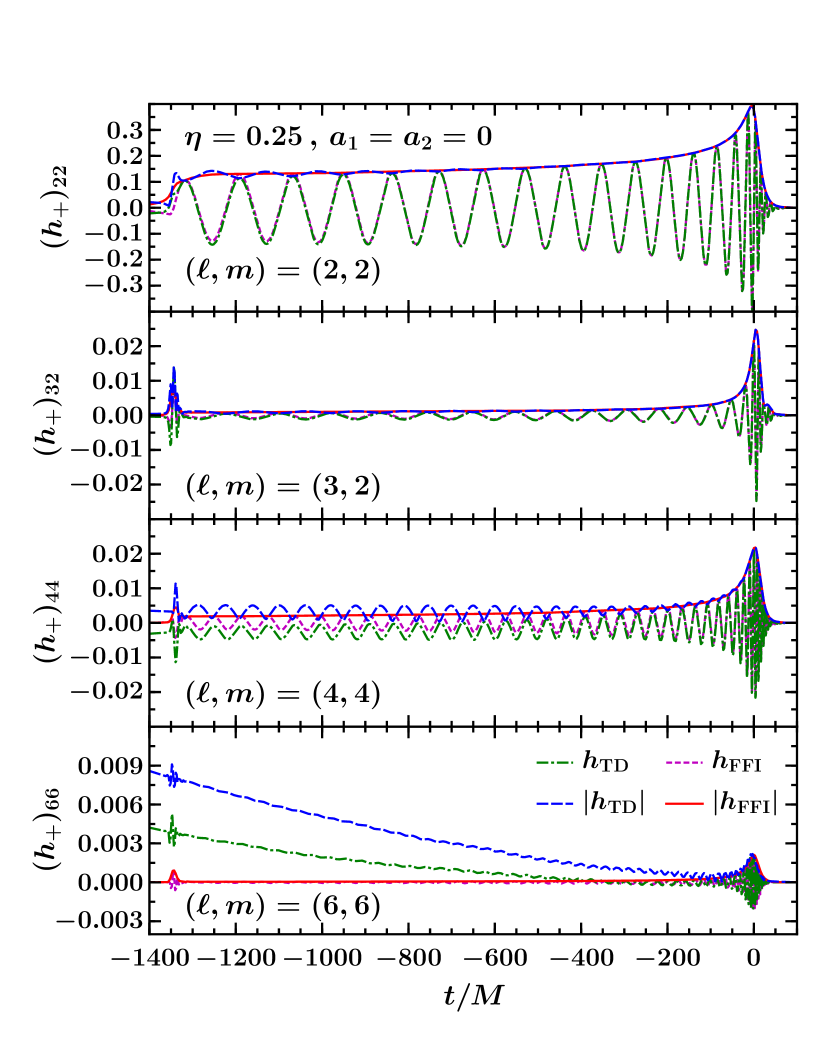
The quality of various integration schemes can be readily seen, if not precisely quantified, in the results of numerically generated waveforms. We present plots from two example models in Figs. 8 and 9.
The first of these is a non-spinning equal mass binary, presented in [34, 35, 19, 20]. We plot four different spherical harmonic modes of the strain, , calculated by integrating which was evaluated during the simulation at future null infinity, . The time series for has a resolution of . In this case, the truncation error appears as high frequency error, effectively resulting in a numerical truncation error of approximately . For this model, we have choosen the integration constants such that the signal becomes zero at late times. Hence, each of the displayed modes is expected to oscillate about zero. However, we notice a slight non-linear drift in the time-domain integrated , computed using a 4th-order Simpson’s rule. The effect of the drift is clearest in the plot of the complex amplitude, , which should grow monotonically, but rather displays oscillations at half the orbital frequency wherever the circularly polarized modes are off-centred. We have integrated the same data using the FFI method. The initial orbital frequency at the start time of the simulation is , corresponding to a wave frequency of in the mode. For the integration procedure, we have used for the and modes, and and for and respectively. The resulting strain shows that drifts have been strongly reduced, while maintaining the overall wave amplitude. (The latter point can be gauged approximately by the fact that the FFI amplitude tracks the average of the oscillations of the TD amplitude in the case, or by shifting the waves and comparing the amplitudes of individual cycles.)
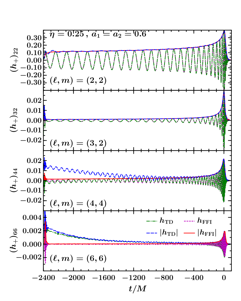
Similar results are apparent in Fig. 9. In this case, the waveform is from a model for which each body has spin aligned with the orbital angular momentum. The sampling rate and truncation error are the same as in the previous model. In this case, the initial frequency of the mode is . For the FFI method, we have used the same as in the non-spinning case, applied to each mode. The integration is most sensitive to the choice of in the early part (first ) of the wave, and late ringdown ( after the peak) when the amplitude approaches the level of the truncation error. By varying the integration parameter between , we find variations of and in the calculated amplitude in these two regions, respectively. However, restricting attention to the range , we find that varying the integration parameter affects the calculated amplitude by less than .
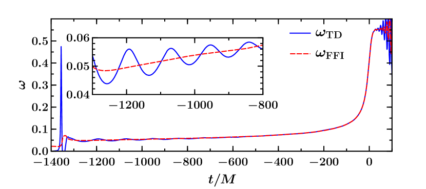
Reduced artificial oscillations are also apparent in other physically important quantities. For instance, Fig. 10 plots the instantaneous frequency, of the integrated computed in the time domain and via FFI. Artificial oscillations in this quantity can be confused with physical eccentricity. Indeed, the FFI result retains small oscillations in , which are consistent with those seen in the raw data, suggesting that the small remaining physical eccentricity modes have been retained, while the artificial non-linear drifts are removed.
Finally, we note that while the artificial integration drifts have a notable visible effect, they seem to have little influence on the use of in a detector template. We can compute the match
| (32aj) |
between the time-domain integrated and , where
| (32ak) |
is a detector dependent scalar product involving the sensitivity curve .
We find that the mismatch, , between time-domain integration and FFI is never greater than for systems less than for Advanced-LIGO, and for LISA. Thus, the effect of integration drift over the length scales considered here is negligible in terms of detection. Nevertheless, it is crucial for constructing appropriate long templates by matching to post-Newtonian models [47, 48].
5 Conclusion
Transforming the variables commonly output by a numerical simulation to the gravitational-wave strain involves some fundamental uncertainties. These artifacts are a result of the integration of finite length, discretely sampled, noisy data. Independent sources of error contribute to large secular non-linear drifts in the integrated data, in particular random-walk effects for time-domain integrations, and spectral leakage in the frequency domain. These effects have nothing to do with the simulation itself, i.e., they are unrelated to gauge or local measurement effects. They are inevitable regardless of the quality of the model (though lowering the level of noise will reduce the effects of random-walk). And they are independent of the genuine integration constants which also arise, but lead at most to a linear drift. The simple prescription which we have developed, FFI, which, given a single parameter , can be applied to any (oscillatory) waveform mode (see [49] for an application in stellar core collapse) suppresses the worst of the problems in the analytic test-cases and numerous practical examples which we have studied, including various spin configurations of binary black hole inspiral. The method involves a single parameter choice, , and removes the bulk of the effect of spectral leakage while maintaining the amplitude of all oscillation modes. A similar effect can be achieved through a careful choice of band-pass filters, though our experience suggests a certain amount of experimentation is required before a similarly satisfactory result can be obtained. This may be impractical for use in parameter space studies involving a large number of physical models and modes.
The issue remains that removing the spurious non-linear drifts associated with integration involves a modification of the data, and in particular potential distortions of low-frequency physical information. Especially, low-frequency information such as the linear and non-linear memory effect will be very hard to disentangle from the “artificial memory” induced by numerical error, since both effects appear as low-frequency drifts in the time domain waveforms. Also, without an exact solution to compare against, it is not possible to arrive at a rigorous estimate of the error in the strain calculated for a given waveform. The examples here suggest that a variation on the order of in amplitude can be expected between different integration methods or parameter choices. This source of error should be taken into account, for instance, in matching post-Newtonian results to numerically calculated strains for the merger.
Finally, we note that while we have emphasized that low-frequency artifacts arise purely due to the process of numerical integration, systematic aspects of the data measurement can still complicate the situation. The results we have presented here use characteristic data measured at , and are free of the coordinate effects discussed in the introduction. Finite-radius extraction can be problematic in a number of ways, related to the local gauge and dynamics of the measurement sphere. But also, specific truncation errors and numerical artifacts may be poorly correlated between measurements at different radii, complicating the extrapolation of integrated quantities. We generally find it preferable to extrapolate and then integrate. The secular drifts in from extrapolated waveforms tend to be more problematic than the characteristic results presented here. However, high-pass filter techniques and FFI are quite effective for such data as well, though with an increased (and difficult to estimate) systematic error due to the finite-radius effects.
References
References
- [1] Frans Pretorius. Evolution of binary black hole spacetimes. Phys. Rev. Lett., 95:121101, 2005.
- [2] Manuela Campanelli, Carlos O. Lousto, Pedro Marronetti, and Yosef Zlochower. Accurate evolutions of orbiting black-hole binaries without excision. Phys. Rev. Lett., 96:111101, 2006.
- [3] John G. Baker, Joan Centrella, Dae-Il Choi, Michael Koppitz, and James van Meter. Gravitational wave extraction from an inspiraling configuration of merging black holes. Phys. Rev. Lett., 96:111102, 2006.
- [4] Thibault Damour, Alessandro Nagar, Ernst Nils Dorband, Denis Pollney, and Luciano Rezzolla. Faithful Effective-One-Body waveforms of equal-mass coalescing black-hole binaries. Phys. Rev., D77:084017, 2008.
- [5] Thibault Damour, Alessandro Nagar, Mark Hannam, Sascha Husa, and Bernd Bruegmann. Accurate Effective-One-Body waveforms of inspiralling and coalescing black-hole binaries. Phys. Rev., D78:044039, 2008.
- [6] Thibault Damour and Alessandro Nagar. An Improved analytical description of inspiralling and coalescing black-hole binaries. Phys.Rev., D79:081503, 2009.
- [7] Alessandra Buonanno et al. Effective-one-body waveforms calibrated to numerical relativity simulations: coalescence of non-spinning, equal- mass black holes. Phys. Rev., D79:124028, 2009.
- [8] Yi Pan, Alessandra Buonanno, Luisa T. Buchman, Tony Chu, Lawrence E. Kidder, Harald P. Pfeiffer, and Mark A. Scheel. Effective-one-body waveforms calibrated to numerical relativity simulations: coalescence of non-precessing, spinning, equal-mass black holes. Phys. Rev., D81:084041, 2010.
- [9] P. Ajith et al. Phenomenological template family for black-hole coalescence waveforms. Class. Quant. Grav., 24:S689–S700, 2007.
- [10] P. Ajith et al. A template bank for gravitational waveforms from coalescing binary black holes: I. non-spinning binaries. Phys. Rev. D, 77:104017, 2008.
- [11] P. Ajith, M. Hannam, S. Husa, Y. Chen, B. Bruegmann, et al. Inspiral-merger-ringdown waveforms for black-hole binaries with non-precessing spins. Phys.Rev.Lett., 106:241101, 2011.
- [12] L. Santamaria, F. Ohme, P. Ajith, B. Bruegmann, N. Dorband, et al. Matching post-Newtonian and numerical relativity waveforms: systematic errors and a new phenomenological model for non-precessing black hole binaries. Phys.Rev., D82:064016, 2010.
- [13] Benjamin Aylott et al. Testing gravitational-wave searches with numerical relativity waveforms: Results from the first Numerical INJection Analysis (NINJA) project. Class. Quant. Grav., 26:165008, 2009.
- [14] Benjamin Aylott et al. Status of NINJA: the Numerical INJection Analysis project. Class. Quant. Grav., 26:114008, 2009.
- [15] Numerical Injection Analysis (NINJA) Project Page.
- [16] John Baker, Manuela Campanelli, Carlos O. Lousto, and Ryoji Takahashi. Modeling gravitational radiation from coalescing binary black holes. Phys. Rev. D, 65:124012, 2002.
- [17] E. Berti, V. Cardoso, J. A. Gonzalez, U. Sperhake, M. Hannam, S. Husa, and B. Brügmann. Inspiral, merger, and ringdown of unequal mass black hole binaries: A multipolar analysis. Physical Review D, 76(6):064034, September 2007.
- [18] Mark Hannam et al. The Samurai Project: verifying the consistency of black- hole-binary waveforms for gravitational-wave detection. Phys. Rev., D79:084025, 2009.
- [19] C. Reisswig, N. T. Bishop, D. Pollney, and B. Szilagyi. Unambiguous determination of gravitational waveforms from binary black hole mergers. Phys. Rev. Lett., 103:221101, 2009.
- [20] C. Reisswig, N. T. Bishop, D. Pollney, and B. Szilagyi. Characteristic extraction in numerical relativity: binary black hole merger waveforms at null infinity. Class. Quant. Grav., 27:075014, 2010.
- [21] Manuela Campanelli, Carlos O. Lousto, Hiroyuki Nakano, and Yosef Zlochower. Comparison of Numerical and Post-Newtonian Waveforms for Generic Precessing Black-Hole Binaries. Phys. Rev., D79:084010, 2009.
- [22] T. Regge and J. Wheeler. Stability of a Schwarzschild singularity. Phys. Rev., 108(4):1063–1069, 1957.
- [23] F. J. Zerilli. Gravitational field of a particle falling in a Schwarzschild geometry analyzed in tensor harmonics. Phys. Rev. D., 2:2141, 1970.
- [24] V. Moncrief. Gravitational perturbations of spherically symmetric systems. I. the exterior problem. Annals of Physics, 88:323–342, 1974.
- [25] Andrew Abrahams and C. Evans. Gauge invariant treatment of gravitational radiation near the source: Analysis and numerical simulations. Phys. Rev. D, 42:2585–2594, 1990.
- [26] Peter Anninos, D. Hobill, E. Seidel, L. Smarr, and W.-M. Suen. The head-on collision of two equal mass black holes: Numerical methods. Technical Report 24, National Center for Supercomputing Applications, 6 1994.
- [27] A. M. Abrahams and R. H. Price. Applying black hole perturbation theory to numerically generated spacetimes. Phys. Rev. D, 53:1963, 1996.
- [28] Denis Pollney, Christian Reisswig, Luciano Rezzolla, Béla Szilágyi, Marcus Ansorg, Barret Deris, Peter Diener, Ernst Nils Dorband, Michael Koppitz, Alessandro Nagar, and Erik Schnetter. Recoil velocities from equal-mass binary black-hole mergers: a systematic investigation of spin-orbit aligned configurations. Phys. Rev., D76:124002, 2007.
- [29] Roger Penrose. Asymptotic properties of fields and space-times. Phys. Rev. Lett., 10:66–68, 1963.
- [30] H. Bondi, M. G. J. van der Burg, and A. W. K. Metzner. Gravitational waves in general relativity VII. Waves from axi-symmetric isolated systems. Proc. R. Soc. London, A269:21–52, 1962.
- [31] R.K. Sachs. Gravitational waves in general relativity VIII. Waves in asymptotically flat space-time. Proc. Roy. Soc. London, A270:103–126, 1962.
- [32] E. Deadman and J. M. Stewart. Numerical Relativity and Asymptotic Flatness. Class. Quant. Grav., 26:065008, 2009.
- [33] John G. Baker et al. Mergers of non-spinning black-hole binaries: Gravitational radiation characteristics. Phys. Rev., D78:044046, 2008.
- [34] Denis Pollney, Christian Reisswig, Nils Dorband, Erik Schnetter, and Peter Diener. The Asymptotic Falloff of Local Waveform Measurements in Numerical Relativity. Phys. Rev., D80:121502, 2009.
- [35] Denis Pollney, Christian Reisswig, Erik Schnetter, Nils Dorband, and Peter Diener. High accuracy binary black hole simulations with an extended wave zone. Phys.Rev., D83:044045, 2011.
- [36] W. H. Press, B. P. Flannery, Saul A. Teukolsky, and W. T. Vetterling. Numerical Recipes. Cambridge University Press, New York, 2nd edition, 1992.
- [37] Michael Boyle et al. High-accuracy numerical simulation of black-hole binaries: Computation of the gravitational-wave energy flux and comparisons with post-Newtonian approximants. Phys. Rev., D78:104020, 2008.
- [38] Timothy S. Edwards. Effects of aliasing on numerical integration. Mechanical Systems and Signal Processing, 21(1):165 – 176, 2007.
- [39] Subrahmanyan Chandrasekhar. Stochastic problems in physics and astronomy. Rev. Mod. Phys., 15:1–89, 1943.
- [40] Alan V. Oppenheim and Ronald W. Schafer. Discrete-Time Signal Processing. Prentice Hall, 3rd edition, 2009.
- [41] Alexander D. Poularikas. The Transforms and Applications Handbook, Second Edition. CRC Press, 2000.
- [42] D. J. A. McKechan, C. Robinson, and B. S. Sathyaprakash. A tapering window for time-domain templates and simulated signals in the detection of gravitational waves from coalescing compact binaries. Class. Quant. Grav., 27:084020, 2010.
- [43] S Butterworth. On the theory of filter amplifiers. Experimental Wireless and the Wireless Engineer, 7:536–541.
- [44] C. D Ott. TOPICAL REVIEW: The gravitational-wave signature of core-collapse supernovae. Classical and Quantum Gravity, 26(6):063001, March 2009.
- [45] Frans Pretorius and Deepak Khurana. Black hole mergers and unstable circular orbits. Class. Quant. Grav., 24:S83–S108, 2007.
- [46] Ulrich Sperhake et al. Cross section, final spin and zoom-whirl behavior in high- energy black hole collisions. Phys. Rev. Lett., 103:131102, 2009.
- [47] Mark Hannam, Sascha Husa, Frank Ohme, and P. Ajith. Length requirements for numerical-relativity waveforms. Phys.Rev., D82:124052, 2010.
- [48] Ilana MacDonald, Samaya Nissanke, Harald P. Pfeiffer, and Harald P. Pfeiffer. Suitability of post-Newtonian/numerical-relativity hybrid waveforms for gravitational wave detectors. Class.Quant.Grav., 28:134002, 2011.
- [49] C. Reisswig, C.D. Ott, U. Sperhake, and E. Schnetter. Gravitational Wave Extraction in Simulations of Rotating Stellar Core Collapse. Phys.Rev., D83:064008, 2011.