Implementation of a simplified approach to radiative transfer in general relativity
Abstract
We describe in detail the implementation of a simplified approach to radiative transfer in general relativity by means of the well-known neutrino leakage scheme (NLS). In particular, we carry out an extensive investigation of the properties and limitations of the NLS for isolated relativistic stars to a level of detail that has not been discussed before in a general-relativistic context. Although the numerous tests considered here are rather idealized, they provide a well-controlled environment in which to understand the relationship between the matter dynamics and the neutrino emission, which is important in order to model the neutrino signals from more complicated scenarios, such as binary neutron-star mergers. When considering nonrotating hot neutron stars we confirm earlier results of one-dimensional simulations, but also present novel results about the equilibrium properties and on how the cooling affects the stability of these configurations. In our idealized but controlled setup, we can then show that deviations from the thermal and weak-interaction equilibrium affect the stability of these models to radial perturbations, leading models that are stable in the absence of radiative losses, to a gravitational collapse to a black hole when neutrinos are instead radiated.
I Introduction
Neutron stars (NS) are a unique astrophysical laboratory to study the microphysics of superdense matter. From their births in a supernova explosion until their deaths in a merger of compact objects or in a gravitational collapse to a black hole (BH), NSs undergo the most extreme physical conditions with respect to density, temperature and composition. For example, the temperature can vary from a surface temperature of a few , during the inspiral of two old NSs in a binary system (BNSs), up to at the time of merger Bauswein et al. (2012). Similarly, a NS can reach up to – times nuclear saturation density Baiotti et al. (2005a). The merger of two NSs is considered one of the most promising astrophysical events in which to test the models of nuclear matter in regimes that are unattainable in laboratory experiments. In addition to the bulk properties of the NSs, such as mass and radius, also the details of the NS equation of state (EOS), are expected to be imprinted in the electromagnetic emission (EM) and gravitational wave (GW) signal produced by these events.
In particular, the GW signal that accompanies the merger of BNSs is expected to be the prime target for the advanced generation of kilometer length ground-based detectors, such as LIGO Abbott et al. (2009), Virgo Acernese et al. (2009), and KAGRA Kuroda et al. (2010). Individual merger signals can reveal the NS radii with an accuracy of km together with their masses Hinderer et al. (2010). These observations will strongly constrain the EOS that describes the NS matter at zero temperature. Moreover, GWs, together with their EM counterparts, will be of great relevance to determine the properties of the engine behind short gamma-ray bursts (GRBs) which are thought to arise from NS/NS and BH/NS mergers Eichler et al. (1989); Rezzolla et al. (2011). The incorporation of microphysical nuclear EOSs, general relativity, magnetic fields, neutrino radiation, viscosity and other transport coefficients in the numerical modeling of those events, is essential to increase the realism of the simulations and help us explore the possible outcomes from a large set of initial conditions and parameters.
A great deal of effort has been spent in the field of nuclear physics on the development of an EOS appropriate to describe the behavior of matter at both supranuclear and subnuclear densities (see Lattimer and Prakash (2001); Haensel et al. (2007) for reviews). Unfortunately, only few constraints on the properties of the EOS are available from relativistic heavy-ion collision experiments and astronomical observations (see Lattimer (2012) for a review on the topic). The recent discoveries of two massive NSs in a binary system with a mass of Demorest et al. (2010); Antoniadis et al. (2013) seem to rule out some of the NS matter models. Nevertheless, the lack of precise estimates of their radii did not allow to significantly reduce the parameter space for the NS EOSs. Combined measurements of mass and radius of NSs can only be obtained from x-ray bursts and from the NS surface thermal emission, something unlikely to happen in quiescent systems as the one described in Demorest et al. (2010) and Antoniadis et al. (2013). These measurements are subject to many uncertainties, as the distance of the NS and its magnetic field, that can spoil the accuracy of the estimates of the radius Özel et al. (2010). More importantly, the estimates of the physical parameters from the observations are sensitive to the models adopted for their analysis Steiner et al. (2010).
As a result of the complexity involved in the theoretical models of NS matter, only few EOSs cover temperatures up to , densities that reach several times nuclear saturation density and a range of composition that goes from pure neutron matter to symmetric matter (equal neutron and proton number, ). Amongst the few EOSs that have gained popularity for astrophysical simulations, particularly well studied are the EOS of Lattimer and Swesty (1991) (hereafter, LS-EOS) and the EOS proposed by Shen et al. (1998a, b). More recently, a new EOS has been derived by Shen et al. (2010, 2011) (hereafter, SHT-EOS), in which the meson mean fields and the Dirac wave function describing the nucleons are solved self-consistently for each Wigner-Seitz cell. Despite the accuracy reached in the theoretical models, these EOSs not always satisfy the constraints imposed by both experiments (symmetry energy and incompressibility) and astronomical observations (mass and radius) Steiner et al. (2010); Hebeler et al. (2013).
Over the last few years, a lot of progress has been made to understand the dynamics of BNS systems in general relativity with respect to the possible detection of GWs from such systems (for a review see Faber and Rasio (2012)). The level of sophistication reached by present-day general-relativistic simulations includes important microphysical aspects Sekiguchi et al. (2011a, b); Bauswein et al. (2012) that in the past were only accessible to Newtonian simulations Ruffert et al. (1996, 1997); Ruffert and Janka (2001); Rosswog and Liebendörfer (2003). Together with nuclear EOSs to describe the NS matter, current approaches also include weak-interaction processes, albeit modeled by means of approximate neutrino treatments. Under the extreme thermodynamic conditions reached during the merger, powerful neutrino bursts are produced from the hot and shock heated NS matter Sekiguchi et al. (2011a). When the nuclear matter is strongly compressed and its temperature reach values of about , weak-interaction processes become increasingly important, leading the material out of the original chemical equilibrium with respect to processes while copious amounts of neutrinos are emitted. Neutrinos are responsible for the luminosities of the order attained in BNS mergers and they may play a role in powering the relativistic jet needed for the beamed emission of a GRB. The energy required for the outflow can be efficiently deposited along the baryon-free axis of rotation of the BH by neutrino pair annihilation Ruffert et al. (1996).
The aim of this paper is to present the details of the implementation in the new Whisky code (WhiskyThermal) Baiotti et al. (2003, 2005b) of a ”neutrino leakage” scheme (NLS) along with state-of-the-art nuclear EOSs with density, temperature and composition dependence. The NLS is a pragmatic approach to neutrino radiation transfer that estimates the local changes in the lepton number and the associated energy losses via neutrino emission. The relative simplicity of the implementation along with the small computational costs turn the NLS into an interesting approach to upgrade numerical relativity codes that evolve the equations of general-relativistic hydrodynamics (GRHD) and magneto-hydrodynamics together with the Einstein equations for a dynamical spacetime.
Neutrino interactions are influenced by density, temperature and composition of the hadronic matter and by the energy of the emitted neutrinos. At rest-mass densities of few times and temperatures around , the scattering of neutrinos onto baryons is so efficient that neutrinos quickly reach the thermal equilibrium with the NS matter and can be considered as trapped (i.e., with mean free path ). When the density drops below , neutrinos with energy below interact rarely with the nuclear matter and can therefore be considered as free-streaming (i.e., with mean free path ). The NLS scheme is particularly suited to study the evolution of a NS because of the sharp density gradient at the surface where the density drops by several orders of magnitude. More accurate schemes such as the direct Monte Carlo method for solving the Boltzmann transport equation Abdikamalov et al. (2012), are able to capture properly the dynamic in the semitransparent regime. Unfortunately, the computational cost involved limits the use of such schemes to one-dimensional problems. Three-dimensional simulations are performed instead using approximate ”ray-by-ray” Scheck et al. (2006) multi-energy-group neutrino schemes [e.g., multigroup flux-limited diffusion Mezzacappa and Bruenn (1993) and isotropic diffusion source approximation Liebendörfer et al. (2009)]. Even more advanced, but still rudimentary, approaches to the solution of the radiative-transfer problem have been presented recently in Ref. Radice et al. (2013).
Besides carrying out an extensive investigation of the properties and limitations of the NLS to a level of detail that, to the best of our knowledge, has not discussed before in a general-relativistic context, we also present novel results regarding the equilibrium properties of nonrotating hot NSs and how the cooling affects the stability of these configurations. In particular, we use several temperature profiles close to the one reached by protoneutron stars (PNSs) during their formation in a supernova core collapse or by the hypermassive neutron star (HMNS) produced in a BNS merger and investigate how the energy losses can influence the stability of these objects. In our idealized but well-controlled setup we can then show that deviations from the thermal and weak-interaction equilibrium of these models will affect their stability to radial perturbations and thus lead to a neutrino-induced collapse of stable nonrotating NS models.
The organization of the paper is as follows: In Sec. II we summarize our mathematical framework regarding the gravitational field equations and the GRHD equations in the presence of neutrino emission. Sec. III describes the neutrino leakage scheme while Sec. IV discusses the nuclear equations of state for NS matter used in this work. Sec. V describes in detail the numerical framework adopted for our simulations. Sec. VI, presents a series of tests and results obtained with our code. In particular, we show simulations of nonrotating stable NS with nuclear EOS at finite temperature and in -equilibrium, comparing with predictions from linear-perturbation theory. Finally, Sec. VII reports the main result of this paper, namely, the neutrino-induced collapse of a stable nonrotating NS and the associated neutrino bursts when using different thermal EOSs. Appendix A reports the details of the free emission rates and opacity sources used in our code and that could be of direct use for anyone wanting to reproduce our implementation, while a detailed description of the convergence tests of our scheme are presented in Appendix B. A detailed description of a novel and robust technique for the transformation from conserved to primitive variables is finally presented in Appendix C. Unless stated otherwise, we use geometrized units in which . Latin indices run from 1 to 3 while greek indices run from 0 to 3.
II Mathematical Framework
Although much of our mathematical and numerical framework for the solution of the Einstein-Euler equations has been presented in a scattered manner in a number of papers, i.e., Baiotti et al. (2005a, 2008), we include a short review here both for completeness and as an aid to anyone wanting to implement our approach to the handling of the radiative transfer.
II.1 Einstein equations
We evolve a conformal-traceless ”” formulation of the Einstein equations Nakamura et al. (1987); Shibata and Nakamura (1995); Baumgarte and Shapiro (1998), BSSNOK. The spacetime is foliated into three-dimensional spacelike hypersurfaces, with a three-metric , extrinsic curvature , and the gauge functions (lapse) and (shift) to specify the coordinate frame. The three-metric is conformally transformed as
| (1) |
and the conformal factor is evolved as an independent variable, whereas is subject to the constraint . The extrinsic curvature is subject to the same conformal transformation and its trace is evolved as an independent variable, while in place of we evolve its conformal-traceless equivalent, i.e.,
| (2) |
with . In addition, new evolution variables defined in terms of the Christoffel symbols of the conformal three-metric are introduced, i.e.,
| (3) |
and solved as independent evolution variables. As a result, the complete set of the evolution equations for the Einstein equations is given by
| (4) | ||||
| (5) | ||||
| (6) | ||||
| (7) | ||||
| (8) |
where is the Lie derivative with respect to the shift vector, is the three-dimensional Ricci tensor, the covariant derivative associated with the three-metric , ”TF” indicates the trace-free part of tensor objects and , , and are the matter source terms defined as
| (9) | ||||
| (10) | ||||
| (11) |
where is the future-pointing four-vector orthonormal to the spacelike hypersurface, is the energy-momentum tensor for a perfect fluid [cf., Eq. (22)], and . The Einstein equations also comprise a set of physical constraint equations that are satisfied within each spacelike slice,
| (12) | ||||
| (13) |
which are usually referred to as Hamiltonian and momentum constraints. Here is the Ricci scalar on a three-dimensional time slice. Our specific choice of evolution variables introduces two additional constraints,
| (14) | ||||
| (15) |
which are enforced on each spacelike hypersurface. The remaining constraints, and are not actively enforced and can be used to monitor the accuracy of our numerical solution.
Our gauge choices reflect the experience matured over the last decade and are already discussed in detail in Baiotti et al. (2008). In particular, we evolve the lapse according to the ”” slicing condition Bona et al. (1995):
| (16) |
where is the initial value of the trace of the extrinsic curvature and equals zero for the maximally sliced initial data we consider here. The shift is evolved using the hyperbolic -driver condition Alcubierre et al. (2003),
| (17) | |||||
| (18) |
where is a parameter which acts as a damping coefficient. Following Alcubierre et al. (2003) and because we are not considering binaries here, we set to be , where is the total gravitational mass of the system; a more sophisticated prescription in case of unequal-mass binaries can be found in Alic et al. (2010).
All the equations discussed above are solved using the McLachlan code, a three-dimensional finite-differencing code based on the Cactus Computational Toolkit Löffler et al. (2012).
II.2 Relativistic-hydrodynamic equations
In the following, we describe the matter evolution equations implemented in the new Whisky code. These are given by the general-relativistic-hydrodynamic equations describing a perfect compressible fluid governed by a generic EOS with temperature and composition dependence. In particular, the changes in composition, energy, and momentum due to neutrino radiation are modeled by introducing additional source terms.
When written in covariant form, the equations for the conservation of energy, momentum, baryon and lepton numbers are expressed as
| (19) | ||||
| (20) | ||||
| (21) |
where and are the baryon and electron number densities, respectively. Note that the energy-momentum tensor accounts for the ordinary matter as well as for the trapped neutrinos and photons, but it does not include the nontrapped neutrinos. The corresponding energy-momentum tensor is taken into account only in the form of the source term modeling the radiative losses of energy and momentum. Furthermore, because we assume these nontrapped neutrinos to behave essentially as a test fluid, the associated energy momentum tensor is neglected when building the right-hand side of the Einstein equations.
As customary in a NLS, also in our implementation we do not evolve directly the number density and the energy distribution of the neutrinos. Instead, since the neutrinos are assumed to be in local thermal equilibrium with the baryonic matter, we can obtain direct estimates for the source terms and by simply considering the matter properties. Also, because we do not consider lepton species other than electrons in our fluid, the only degree of freedom in the composition is represented by the electron fraction defined as . The electron fraction is changed only by the production of electron neutrinos and antineutrinos as described by the source term .
The energy-momentum tensor used in Eq. (19) is that of a perfect fluid, given by
| (22) |
where is the baryon rest-mass density defined as , where denotes the nucleon mass111 The formal nucleon mass is chosen differently for each EOS, such that . In detail, for the LS-EOS, and by for the SHT-EOS.. The total isotropic pressure and the total specific internal energy contain contributions of baryons, electrons, photons, and trapped neutrinos
| (23) | ||||
| (24) |
where the contribution from trapped electron-neutrinos and antineutrinos in the dense baryonic component can be evaluated from the thermodynamic state of the fluid and assuming that the neutrinos are following a Fermi-Dirac distribution, i.e.,
| (25) | |||||
| (26) |
Here, and are the degeneracy parameters for the electron-neutrinos and antineutrinos, the corresponding chemical potentials, is the temperature, which is expressed in throughout the paper, and is a Fermi integral [see Eq. (79) and Appendix A for a more extended discussion]. Note also that in Eq. (23) the electron contributions to the total pressure and internal energy are computed using the EOS for a semidegenerate gas of electrons as described in Ref. Timmes and Swesty (2000).
At rest-mass densities and temperatures , the contributions can be significant and around of the baryonic one. However, close to nuclear saturation density, it becomes less than of the total pressure and thus smaller than the typical uncertainties of the nuclear EOSs at such densities. Furthermore, the addition of a neutrino isotropic pressure to the fluid pressure is meaningful only in the trapped regime and cannot be made when the neutrinos are free streaming. For these reasons and to maintain a smooth transition between the regimes of trapped and free-streaming neutrinos, we neglect contributions of trapped neutrinos to pressure and internal energy, setting in Eqs. (23)–(24).
To compute the neutrino source term in Eq. (21), which describes the changes in electron fraction, we introduce the neutrino emission rates per baryon, and , for electron-neutrinos and -antineutrinos, respectively. As a result, in the fluid rest frame we can express the change in electron fraction as
| (27) |
Similarly, in order to determine the source terms describing the radiative losses of energy and momentum due to neutrinos in Eq. (19), we assume that the emission is isotropic in the fluid rest frame, so that no net momentum change can take place in the rest frame. We then obtain the following covariant equation that can be most easily verified in the comoving frame
| (28) |
where we have introduced the neutrino emissivity as the sum of the emissivities of the various neutrino species with , which denote the radiated energy per unit time and baryon (i.e., it is expressed as in cgs units). Note that we collect the emissivity due to the and neutrinos into a single contribution . An important remark should be made about Eq. (21). Since the neutrino interaction time scale depends largely on the microphysics of the process described, it can differ significantly from the time scale over which the baryonic matter evolves, resulting in a problem with a stiff source term. When this happens, special numerical algorithms are needed to handle the evolution (see, e.g., Palenzuela et al. (2009)).
For numerical evolution, the equations are cast into a flux conservative formulation, based on the Valencia formulation originally developed by Martí et al. (1991); Banyuls et al. (1997). In particular, we write Eqs. (19)–(21) as balance laws
| (29) |
where is the determinant of the three-metric, while and are the flux vectors and source terms, respectively (see Font (2008) for details). The right-hand side contains the geometrical terms and the neutrino reaction rates that depend on the state of the fluid. The evolved conserved variables are given in terms of the primitive variables via the relations
| (30) | ||||
| (31) | ||||
| (32) | ||||
| (33) |
In the equations above, is the three-velocity measured by an observer orthogonal to the hypersurface of constant coordinate time (i.e., a Eulerian observer), is the corresponding Lorentz factor, and is the specific enthalpy. When written out explicitly, Eq. (29) reads
| (34) | ||||
| (35) | ||||
| (36) | ||||
| (37) | ||||
where , , , , , and denotes the advection speed with respect to the coordinates.
In order to close the system of equations, we need an EOS to relate the pressure to the rest of the primitive quantities (see Sec. IV). The new Whisky code implements several analytic EOSs, such as the polytropic EOS, the ideal-fluid (-law) EOS, as well as ”hybrid” EOSs Janka et al. (1993). Finally, the code can use microphysical finite-temperature EOSs in tabulated form to describe nuclear matter and the neutrino interactions, as will be discussed in Sec. IV.
The following sections are devoted to a description of our treatment of the radiative transport within the NLS and of the interactions between neutrinos and ordinary matter when the latter is modeled with the nuclear EOS described in Sec. IV.
III Approximate radiative transfer: the neutrino leakage scheme
Neutrinos from hot, dense and neutron-rich nuclear material are produced via nonequilibrium weak-interaction processes during the first minutes (or months) of the life of a PNS and in the final stages of the merger of BNSs, when a HMNS is produced. The cooling produced by these neutrinos and the consequent influence on the stellar structure and equilibrium is of course of great importance to model these processes accurately. In order to study the possible influence of thermal effects on the onset of dynamical instabilities in PNSs or HMNSs, it is necessary to evolve the system for tens of dynamical time scales, which can be estimated to be ms, where and are the mass and size of the object. This time scale is short when compared with the typical diffusion time scale of neutrinos in dense matter, which is s. As a result, it is reasonable to use as a first approximation to the radiative transfer a simple leakage scheme that estimates the instantaneous energy loss via neutrino emission and by the total change in electron fraction of the nuclear matter. Clearly, this represents only a first step towards more sophisticated and accurate transport schemes such as those employed in stellar-core collapse simulations Scheck et al. (2006); Marek and Janka (2009); Liebendörfer et al. (2009); Abdikamalov et al. (2012).
The NLS was originally developed by van Riper et al. van Riper and Lattimer (1981), to describe the neutrino cooling through weak interactions during the core-collapse phase of a supernova. In Newtonian gravity, it was first applied in BNS simulations by Ruffert et al. Ruffert et al. (1996, 1997); Ruffert and Janka (1999, 2001) and more recently by Rosswog et al. (Rosswog and Davies, 2003; Rosswog and Liebendörfer, 2003; Rosswog et al., 2003). It has undergone a revival in general-relativistic three-dimensional supernova simulations with the work of Sekiguchi (2010) and O’Connor and Ott (2010); Ott et al. (2012, 2013) (see also Peres et al. (2013)). Finally, the NLS was also used recently to describe the neutrino cooling in general-relativistic BNS simulations (Sekiguchi et al., 2011a, b) and BH-NS mergers Deaton et al. (2013). The details of the implementation of the NLS differ among these authors and are sometimes fragmentary. For these reasons, and to help anyone wishing to reproduce our implementation, we give below a detailed account of our treatment.
In our scheme we account for three different neutrino species: electron neutrinos , electron-antineutrinos and heavy lepton neutrinos, that are considered as a single component with a statistical weight of 4. The creation of electron-neutrinos and antineutrinos by processes involving neutrons () and protons () leads to changes in the electron number, i.e.,
| (38) | |||
| (39) |
that need to be taken into account. On the other hand, all three species of neutrinos and antineutrinos are created by annihilation of electron-positron pairs, i.e.,
| (40) | |||
| (41) |
and, especially at high temperatures, by plasmon decay, i.e.,
| (42) | |||
| (43) |
In order to compute the emission coefficients, we assume that the neutrinos are massless and in thermal equilibrium with the surrounding matter. As a result, the energy spectrum of the neutrinos follows a Fermi-Dirac distribution for ultrarelativistic particles at the temperature of the matter. A further assumption concerns the chemical potentials of the electron-neutrinos and of the electron-antineutrinos, which are assumed to be at -equilibrium Rosswog and Liebendörfer (2003), i.e.,
| (44) |
where , , are the relativistic chemical potentials including the rest-mass of the particle. As a result, we can define , where now and we assume since the heavy neutrinos are only weakly interacting with the matter. The detailed derivation of the number and energy rates for the different emission processes is described in detail in Appendix A.
As mentioned in the Introduction, low-energy neutrinos (i.e., with ) interact very rarely at low densities, i.e., for . In this regime, if is the mean free path of a neutrino, the time needed by a neutrino of species to cross a slab of nuclear matter of depth , is simply given by
| (45) |
where, we recall, . In this limit, the amount of energy loss by neutrinos can be directly computed using the free emission rates (see below and Appendix A for details). On the other hand, at high densities, i.e., for , the scattering and absorption of neutrinos onto baryons is extremely efficient already for neutrinos with and a purely diffusive regime can be reached, where . Under these conditions, neutrinos cannot freely escape but can only diffuse via a random walk over a time scale
| (46) |
where is a coefficient depending on the optical depth evaluated along the direction of propagation Mihalas and Mihalas (1984). In order to compute the total mean free path, in our NLS we take into account scattering and absorption processes between neutrinos and the surrounding matter. In particular, for the calculation of the opacities we include the following processes:
-
•
coherent neutrino scattering on heavy nuclei (with atomic mass number )
(47) (48) -
•
neutrino scattering on free nucleons
(49) (50) (51) (52) -
•
electron-flavor neutrinos absorption on free nucleons
(53)
Summing all the various contributions to the mean free paths , we define the optical depth simply as the integral of the inverse of the mean free path along a line of sight which is specifically chosen for the geometry of the problem, i.e.,
| (54) |
where is the neutrino energy (see Appendix A for details), and is the proper length. Note we have to neglect the gravitational redshift of the neutrinos, as well as special-relativistic corrections due to the velocity of the absorbing matter. The knowledge of the optical depth has two important applications. First, it can be used to determine the extent of the optically thick regions, which are clearly different for different neutrino species. Second, it can be used to estimate the time scale a neutrino needs to diffuse out of the dense matter region. A simple estimate can be obtained from Eq. (46) by replacing with the optical depth , yielding
| (55) |
This expression is also derived in Ref. Rosswog and Liebendörfer (2003) from a one-dimensional stationary diffusion model, and a similar formula is used by Ref. Ruffert et al. (1997). Results obtained from those prescriptions have been compared with a neutrino flux-limited diffusion transport scheme discussed in Ref. Baumgarte et al. (1996), providing also a calibration of the geometry parameter, which takes a value . Ref. Rosswog and Liebendörfer (2003) also proposes an alternative recipe given by
| (56) |
In practice, it is hard to assess which of the two prescriptions is the most realistic one. The first one has the advantage that the energy dependency can be factored out, which will be crucial for the NLS described below. Considering the approximate nature of the NLS and the fact that the coefficient is itself determined empirically, we use hereafter only the prescription (55).
It should also be noted that the time scale over which our simulations are performed is typically at least 1 order of magnitude smaller than the typical diffusion time scale on which the neutrinos escape from the NS dense core, i.e., s. As a result, the contribution of the diffusive leakage of neutrinos is expected to be much smaller than the abundant emission of neutrinos at densities below the ones of the neutrinosphere. For this reason, the NLS can be considered as a reasonable first approximation to treat neutrino effects without resorting to more sophisticated transport schemes.
As shown in Appendix A, we can separate algebraically the neutrino energy dependence from the mean free path, introducing an inverse mean free path which does not depend on the energy, i.e.,
| (57) |
Similarly, we can define an energy-independent optical depth as
| (58) |
Using Eq. (55), we can now also factor out the energy dependence from the diffusion time scale. With these definitions, we can finally compute the diffusive number and energy emission rates per baryon as
| (59) | ||||
| (60) |
where, we recall, we assume the neutrino number densities to be described by the Fermi-Dirac distribution for ultrarelativistic particles. The integrals over energy can then be carried out analytically. The diffusive emission rates (59) and (60) approximate the real emission rates only in the diffusive regime. We will use them below in a prescription interpolating between optically thin and optically thick regimes.
The assumption of chemical equilibrium also impacts the opacities and the radii of the neutrinospheres, which are in general slightly overestimated in our approach. More specifically, as the region transparent to neutrinos is approached, the chemical potentials tend to vanish as a result of the decreased interaction of the nuclear matter with the neutrino flow. Clearly, this behavior cannot be reproduced when adopting the assumption of chemical equilibrium and in Ref. Ruffert et al. (1997) this problem was overcome by using an iterative procedure that adjusted the chemical potential of the neutrinos between the two regions. Here we follow instead the approach suggested more recently in Ref. Rosswog and Liebendörfer (2003) and use a simple interpolation of the emission rates at chemical equilibrium between the purely diffusive regime and the free-streaming one. This approach simplifies considerably the numerical scheme, allowing us to tabulate all the emission rates and opacities, leaving the computation of the optical depth as the only operation to be performed during the evolution (see Appendix A for details).
As a result, using the free neutrino emission rate per baryon, , and neutrino luminosity per baryon, , and the corresponding quantities for the diffusive emission and , we can now compute the effective rates, and via the following interpolation formulas
| (61) | |||||
| (62) |
Alternatively, we have also implemented a more elaborated interpolation technique as suggested in Sekiguchi (2010)
| (63) | |||||
| (64) |
This new prescription does not seem to lead to significant changes but we reserve a more careful comparison of the two prescriptions to future work.
After computing the effective emission rates, we can define a quantity that will be very useful as a diagnostic tool to estimate where the neutrino cooling is most effective. In particular, for each neutrino species, we define as the neutrinosphere the surface at which
| (65) |
Clearly, inside this region the neutrino cooling is strongly suppressed and the time scale of the emission is dominated by the diffusion processes. Note that other definitions are possible and sometimes the neutrinosphere is defined as the surface at which the spectrally averaged optical depth is equal to (see, for instance, Rosswog and Liebendörfer (2003)).
Finally, the interpolated quantities can then be used to compute the net emission rate per baryon appearing in Eq. (37)
| (66) |
and the luminosity per baryon appearing in Eqs. (35)–(36)
| (67) | ||||
where are the emission rates from proton capture (), the emission rates from electron capture (), while and are the emission rates per unit mass from pair annihilation and plasmon decay, respectively. For the sum over these last two rates, here our notation is compact but not perfect; indeed the term in Eq. (67) should be read as
| (68) |
and the same for the plasmon-decay rates.
While the assumption of chemical equilibrium can be considered natural in the view of the many approximations already taken in a NLS, we should also caution that this assumption could overestimate considerably the emission rates, especially in the transition between the optically thin and thick region.
The effective local neutrino source terms are also used to estimate the total luminosity as the neutrino energy that is emitted between the coordinate times and , where the neutrino energy emitted at each point is the one measured by a local coordinate observer with worldline tangent to the four-vector . This observer is somewhat arbitrary, unless the spacetime is stationary with Killing vector . In this case, and assuming no further interactions, the energy of a neutrino measured by such observer is related to the energy measured when the neutrino reaches infinity by the simple relation , regardless of the direction of the emission. To compute the local luminosity, we use the effective emission rates, which are such that the contributions from the optically thick regions are strongly suppressed. The emission rates are given in the fluid rest frame, where a 4-momentum is emitted isotropically per baryon and unit proper time . Such a 4-momentum corresponds to an energy which is measured by our coordinate observers. The relation between the fluid proper time and the coordinate time is , and the number of baryons per coordinate volume is . Using these expressions, we define for each neutrino species the ”source luminosity” , which does not take into account the gravitational redshift, as
| (69) |
where the integral is taken over the whole computational domain, and . In addition, we can compute the luminosity observed at infinity, , by replacing in Eq. (69) with , so as to account for the gravitational redshift. The expression for is strictly valid only for a stationary spacetime with Killing vector . For our nonrotating stationary stellar models, and thus . We will adopt this expression also for oscillating NSs, in which case the dominant error is caused by the fact that a significant fraction of the emitted neutrinos, even those emitted in the free-streaming regime, will hit the NS core and never reach infinity. This could easily reduce the luminosity by a factor around two.
IV Nuclear equations of state for neutron-star matter
The importance that the EOS has in our understanding of the properties of NSs is so large that its study requires no justification. Besides determining the composition and structure of NSs, the EOS also plays a fundamental role in defining the properties of the GW signal that is expected to be produced by NSs, either when isolated or in a binary system. A number of studies about the inspiral and merger of BNS have made this point very clearly, both when the EOS was idealized and analytic, e.g., Baiotti et al. (2007, 2008); Rezzolla et al. (2010), or when more realistic ones were considered, e.g., Freiburghaus et al. (1999); Shibata et al. (2005); Bauswein et al. (2010). Unfortunately, however, our knowledge of matter at nuclear densities is still plagued by too many uncertainties, making it impossible to derive, from robust first principles, what is the most realistic EOS for NS matter. These uncertainties leave ample room for a large variety of possible models for the nuclear matter at zero temperature, which is only mildly constrained by astronomical observations.
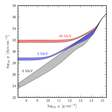
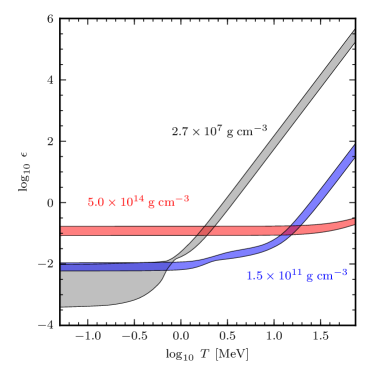
In practice, however, only a few nuclear EOSs are able to encompass the wide range of temperatures, compositions and rest-mass densities necessary to describe matter in supernova explosions and BNS mergers. Here, we will make use of two nuclear EOSs for hot dense matter: the Lattimer-Swesty (LS) EOS Lattimer and Swesty (1991), that adopts a compressible liquid drop model with Skyrme interaction Tondeur et al. (1984), and the Shen-Horowitz-Teige (SHT) EOS, that adopts a relativistic mean-field model for uniform matter with a modified NL3 set of interaction parameters (see Refs. Shen et al. (2010, 2011)). These two EOSs do not include contributions from exotic matter like quarks, hyperons, and kaon or pion condensates. Furthermore, they assume charge neutrality.
In these publicly available EOSs, the pressure and the specific internal energy are given as a function of three independent variables: the baryon number density , the electron/proton fraction , and the temperature . The SHT-EOS is given in a tabulated form, while the LS-EOS is provided in form of computer routines, which provide several choices for the incompressibility modulus, namely . For our simulations we concentrate on a value and cast also the LS-EOS into a tabular form using the routines described in Ref. O’Connor and Ott (2010). Note that the original table for the SHT-EOS has a fairly low resolution and we compensate this by computing a larger table via a thermodynamically consistent interpolation of the Helmholtz free energy Swesty (1996); Timmes and Swesty (2000). In a separate table the SHT-EOS provides also the slice. Since we store the logarithm of the temperature, we cannot use directly this slice, but we use it to extend the original temperature range via linear interpolation. In Table 1, we summarize the ranges covered by the two EOS tables used in our simulations and their resolution.
When it comes to the range in composition, the SHT-EOS can describe the properties of pure neutron matter, that is , but this case is provided as a separate table. To compute a regularly spaced table covering the full range, we fill the gap into the original table using a third-order polynomial interpolation. For the LS-EOS, on the other hand, the smallest available value for the electron fraction is and is taken from the table described in Ref. O’Connor and Ott (2010), and as produced by the routines provided by the LS-EOS. The regime of low electron fraction becomes relevant for NSs at low temperature and -equilibrium, which show a pronounced dip in the electron fraction at the rest-mass densities typical of the inner crust i.e., –.
| EOS | SHT-NL3 | LS-220 |
|---|---|---|
| Number of points in | ||
| Number of points in | ||
| Number of points in |
We note that the original table for the SHT-EOS contains some problematic regions where derived quantities, such as the speed of sound , are extremely noisy or even unphysical. Since our numerical evolution scheme requires a well-behaved sound speed, an additional smoothing step was necessary to remove these irregularities. In particular, we compute the sound speed at constant composition as
| (70) | ||||
where the required derivatives are computed using the limiting procedure described in Steffen (1990). On the other hand, the sound speed for the LS-EOS can be computed analytically from the derivatives of the Helmholtz free energy, yielding smoother results.
| Model | EOS | Spacetime | |||||||||||||
| ] | |||||||||||||||
| sTOV-CW1 | LS-220- | – | fixed | – | |||||||||||
| sTOV-FW1 | LS-220- | – | – | – | – | – | evolved | – | |||||||
| sTOV-CW2 | SHT- | – | fixed | – | |||||||||||
| sTOV-SHT | SHT- | – | – | – | fixed | ||||||||||
| uTOV-LS | LS-220- | – | – | – | – | – | – | – | evolved | ||||||
| uTOV-SHT | SHT- | – | – | – | – | – | – | – | evolved | ||||||
| mTOV-SHT | SHT- | – | – | – | – | – | – | – | evolved | ||||||
| uTOVh-SHT | SHT- | – | – | – | – | – | – | – | evolved | ||||||
Both the LS-EOS and the SHT-EOS tables provide the necessary microphysical quantities to compute the neutrino interactions such as the nucleon and electron chemical potentials, the abundances of heavy nuclei and alpha particles, the proton to nucleon ratio , and the atomic mass number for the ”representative” heavy nuclei.
Fig. 1 illustrates the dependence of the pressure and specific energy as a function of the three independent variables for the SHT-EOS (the LS-EOS shows a similar behavior). The left panel shows the pressure as a function of the rest-mass density for three different temperatures (distinguished by different colors), while the right panel shows the specific internal energy as a function of the temperature for three different densities. Both panels report the influence of the electron fraction as shaded regions that represent the variation over the whole range of . As one can see, the influence of the composition on the pressure is quite large at low temperatures and densities below the crust-core transition, i.e., at . In the core region, on the other hand, the pressure is relatively unaffected by changes in composition and temperature. Note also that the specific internal energy becomes almost temperature independent at densities larger than nuclear saturation density, in stark contrast with simplified analytic EOSs such as the -law EOS.
We recall that the numerical scheme we use to solve the relativistic-hydrodynamic equations provides us at each time step with the rest-mass density , the electron fraction , and internal energy , but not the temperature . The EOS tables, on the other hand, use and as independent variables. As a result, a conversion is needed between and for any given couple of . This is done during the evolution by a discrete bisection algorithm that finds the nearest tabulated temperatures and then performs a linear interpolation.
At regions with high density but low temperature, the conversion becomes very inaccurate because of the very weak dependence of on (cf., right panel of Fig. 1), with the consequence that small errors in can be strongly amplified. Fortunately, this does not affect the hydrodynamic evolution since the pressure shows the same weak dependence on temperature. On the other hand, the local neutrino emission rates do depend strongly on the temperature, i.e., as , so that the free and the effective emission rates can be computed with a large relative error. Luckily, also in this case the errors do not have a serious impact because under these high-density conditions the neutrinos are trapped and the resulting effective luminosity is small. As a result, the influence of inaccurate emission rates on the total luminosity is small as long as the latter is dominated by the emission from hot matter outside the optically thick region.
V Numerical Framework
Much of our numerical infrastructure has been discussed in other papers, e.g., Baiotti et al. (2008); Rezzolla et al. (2010), to which we refer the interested reader for details. Below, we only give a brief overview on the numerical methods used. For the time integration of the coupled set of the hydrodynamic and Einstein equations we use the method of lines (MOL) in conjunction with an explicit fourth-order Runge-Kutta method. In all our simulations we prescribe a Courant-Friedrichs-Lewy (CFL) factor of to compute the time step. The Einstein equations are spatially discretized using a fourth-order finite-difference operator, implemented by the publicly available McLachlan code. The hydrodynamic equations, on the other hand, are discretized in space using a finite-volume scheme based on a piecewise parabolic reconstruction (PPM) Colella and Woodward (1984) and the Harten-Lax-van Leer-Einfeldt (HLLE) Harten et al. (1983) approximate Riemann solver. Differently from the original PPM implementation reported in Ref. Baiotti et al. (2007), we reconstruct here the quantities instead of the three-velocities . This guarantees that the velocities reconstructed at the cell boundaries remain subluminal even under extreme conditions like those encountered near the central region of a BH. As is customary when solving the relativistic-hydrodynamic equations, the vacuum regions are treated by enforcing an artificial atmosphere with a rest-mass density and temperature close to the lowest values covered by the EOS considered (see Table 1) and with a constant electron fraction of .
A discussion on the global convergence order of the simulations reported here is presented in Appendix B and is generally of order –, in agreement with what was found also in previous calculations using the same code with ideal-fluid EOS Baiotti et al. (2009).
V.1 Adaptive-mesh refinement and singularity handling
The use of mesh-refinement techniques is of fundamental importance in our simulations. For this reason, we use the Carpet driver that implements a vertex-centered adaptive-mesh-refinement scheme adopting nested grids Schnetter et al. (2004). For the evolution of isolated NSs presented in this work, it is sufficient to use a fixed hierarchy of nested boxes centered around the origin, with a 2:1 refinement factor between successive grid levels.
In some of the simulations presented here, the final state of the evolution is a BH. We then use the isolated horizon framework Thornburg (2004) to measure its properties every few time steps. We do not make use of the excision technique Baiotti et al. (2005b) in our simulations, neither for the spacetime variables nor for the fluid. As described in Refs. Baiotti and Rezzolla (2006); Baiotti et al. (2007), in order to extend the simulations well past the BH formation, we add a small amount of dissipation to the evolution equations for the metric and gauge variables and rely on the singularity-avoiding gauge (16) (note that no dissipation is added to the evolution of matter variables). More specifically, we use an artificial dissipation of the Kreiss-Oliger-type Kreiss and Oliger (1973), i.e., we augment the right-hand side of the evolution equation of a given quantity with a term , where is the grid spacing. The dissipation is active on the whole computational domain with constant strength . The use of a numerical viscosity is necessary because all the field variables develop very steep gradients in the region near the BH center. Under these conditions, small high-frequency oscillations can lead to instabilities if not dissipated.
V.2 optical depth grid
Different prescriptions are possible in order to estimate the optical depth that is needed in the NLS. A simple choice would be to perform the integrals (58) along the Cartesian coordinate lines and then take the minimum value over all directions. A better choice is to calculate the integrals along directions that are better adapted to the underlying geometry of the matter distribution. In this respect, since we are mainly interested in objects with an overall spherical geometry, a spherical polar coordinate system is better suited than a Cartesian one. Hence, we introduce a spherical grid and compute along a number of a radial coordinate directions the integrals of the energy-independent optical depths , i.e.,
| (71) |
where is the energy-independent part of the inverse mean free path (given in Appendix A). The spherical grid is uniform and we interpolate the three-metric and the opacities from the Cartesian grid hierarchy onto the spherical grid. Next, we integrate from an outer radius , which is large enough to ensure that the region further out is always optically thin, down to . As we march inwards, we store the result of the integrals on the various radial grid points as the intermediate values can be useful to determine, for example, the location of the neutrinospheres. Thanks to this reversed integration direction, it is not necessary to compute the integrals (71) from each point to separately, but only once from to for each angular coordinate on the grid. Once the energy-independent optical depths are known for each point on the spherical grid, they are linearly interpolated back onto the Cartesian grids, where they are used to compute the effective emission rates from the local emission rates according to the NLS prescription (see the discussion in the previous Section).
To reduce computational costs and simplify the implementation, the procedure described above is performed only at each evolution step of the coarsest refinement level. In Appendix B we show that the error caused by the assumption of slowly varying optical depth is negligible for the case of a collapsing NS. In our implementation, the radial spacing of the spherical grid roughly coincides with the spacing on the finest Cartesian grid, and the spherical grid is large enough to cover entirely the finest Cartesian grid. We note that although it would be easy to use a nonregular grid spacing which is much finer near the radiating regions, the accuracy would still be limited by the resolution of the Cartesian grids. Furthermore, the resolution of the spherical grid is essentially limited by two factors. First, by the scalability to a large number of CPUs, since only the interpolation back to the Cartesian grids is implemented in a fully parallel way, while the interpolation to the spherical grid is not. Second, by the available memory on each compute node, since the whole spherical grid needs to be kept in the memory of each parallel process.
VI Tests of the NLS: stable and unstable stars
In the following we present the results of several tests to assess the stability and accuracy of our code when implementing the NLS. In these simulations we cover several astrophysical scenarios from quasiradial oscillations of nonrotating relativistic stars in fixed spacetimes and in full general relativity (Sec.. VI.1 and VI.2), to the gravitational collapse of hot NSs to a BH (Sec. VI.3).
VI.1 Cold stars: Radial oscillations
We start our battery of tests by considering the radial oscillations of nonrotating cold NSs. The cold models are not expected to radiate and are evolved without NLS. First, we test only the hydrodynamic part by using the so-called Cowling approximation, that is, the spacetime is not evolved, but set to the solutions of the Tolmann-Oppenheimer-Volkoff (TOV) equations Misner et al. (1973) describing a stationary NS.
We should remark that the evolution of a NS in hydrostatic equilibrium is frequently used as a test for general-relativistic-hydrodynamics codes (Shibata, 1999; Font et al., 2002; Duez et al., 2003) and general-relativistic MHD codes (Giacomazzo and Rezzolla, 2007; Cerdá-Durán et al., 2007). Despite the relative simplicity and the well-developed theory of linear-perturbations describing such configurations, this test in the presence of radiative emissions is particularly delicate for a nonlinear evolution code like Whisky, not specifically suited to study equilibrium configurations as those considered in Kastaun (2006).
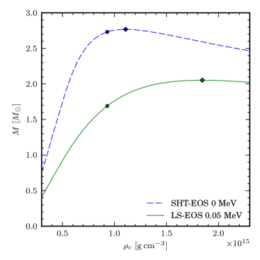
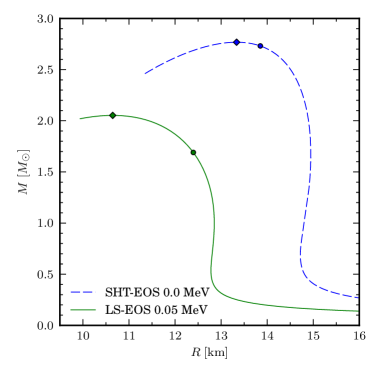
We start by analyzing the radial oscillations of NSs initially in -equilibrium with the lowest temperature available in our EOS tables ( for the LS-EOS and for the SHT-EOS ). Integrating the TOV equations for several central densities, we obtain the relationships between the mass and the radius, and between the mass and the central rest-mass density as plotted in Fig. 2. Note that probably because of the difference in the symmetry energy between the two EOSs, the SHT-EOS yields models that are systematically less compact. For example, for a NS model the SHT-EOS gives a radius that is larger than that of the LS-EOS. Also, because the SHT-EOS is a particularly ”stiff” EOS, the corresponding maximum mass is significantly larger than for the LS-EOS. Interestingly, even for a NS with , the central rest-mass density is only a few times that of the nuclear-matter density .
For our tests we choose two TOV models, one for each EOS, situated on the stable branch with identical central rest-mass density of . Their properties are reported in Table 2 as models sTOV-CW1 and sTOV-CW2. The tests are performed using a grid with two levels of refinement and a spatial resolution on the finest grid of , while the size of the computational domain is . In order to cover the star completely with the finest refinement level, we use 100 points for the model sTOV-CW1 and 120 points for model sTOV-CW2, with the coarser levels containing the same number of points.
The initial equilibrium configurations are perturbed through the injection of the fundamental quasiradial -mode in one case, and of the first radial overtone in the other. The necessary eigenfunctions are computed under the assumption that the EOS used to construct the background model is also valid during the oscillation, which in our case implies the approximation that the -equilibrium holds in the perturbed model. The amplitude of the initial velocity perturbation is and thus still in the linear regime.
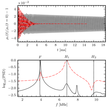
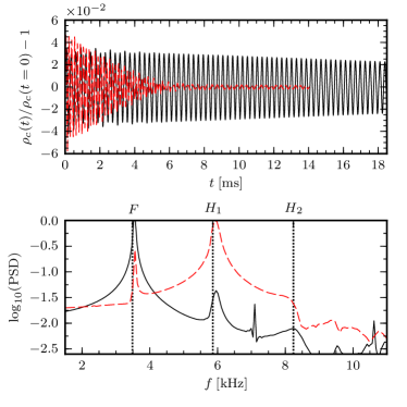
In the top panels of Fig. 3 we show the evolution of the central rest-mass density, for the two EOS considered, LS-EOS (left panels) and SHT-EOS (right panels). We observe the presence of a significant damping in the oscillations, especially for the model perturbed with the -mode (red solid lines in Fig. 3) for which the eigenfunction has a node closer to the surface of the star when compared to the -mode (black solid lines in Fig. 3). This is a purely numerical effect and can be mainly attributed to the treatment of the stellar surface Kastaun (2006). The amplitude of this numerical damping is comparable with the one found by other codes using similar numerical methods for the evolution of the hydrodynamic equations Baiotti et al. (2005a); Dimmelmeier et al. (2006). The use of an artificial atmosphere to approximate the vacuum region outside the NS, in fact, leads to small spurious standing shocks which increase the internal energy at the surface. This artificially heated region hardly affects the global dynamics of the star, but it has a sizeable effect in terms of the total neutrino luminosity.
This is caused by the steep increase of the local neutrino emission rates with temperature, which we recall are proportional to . The surface heating therefore results in a large and unphysical neutrino emission from the surface of the NS, which is not suppressed because the affected regions are optically thin. This problem is somewhat inevitable within a NLS because of the intrinsic assumption of thermal equilibrium between nuclear matter and neutrino radiation. In order to estimate the amount of this emission, we also evolve model sTOV-CW1 with activated NLS. During the evolution, the maximum neutrino luminosity reaches , which should therefore be considered as the minimum luminosity that can be modeled using our scheme.
After evolving for , we compute the Fourier transform of the maximum rest-mass density timeseries (lower panels in Fig. 3) to obtain the frequencies of the stellar pulsations. For each model we also solve the linearized perturbation equations in the Cowling approximation as an eigenvalue problem in order to compute the full spectrum of eigenfunctions. In Table 2 we compare the frequencies extracted from the dynamical evolution of the models with the prediction of the linear-perturbation theory. Remarkably, the difference for the fundamental mode and the first overtone of both EOS models stays within . The accuracy is similar to the results in Baiotti et al. (2005a) for the evolution of a polytropic EOS, giving us confidence in the correctness of our implementation. Interestingly, we note also the presence of other frequencies not predicted by the linear theory. This is the case for the peaks in the PSD that are located at exactly twice the frequencies of the respective -mode, i.e., around for the SHT-EOS and for the LS-EOS. We conjecture that they are caused by nonlinearities in the oscillations that are captured by the evolution code, as it is typical of physical systems governed by nonlinear equations in the limit of small oscillations Landau and Lifshitz (1976); Zanotti et al. (2005).
For the model with the LS-EOS we also perform a run in full general relativity, i.e., model sTOV-FW1 in Table 2. As expected (see Dimmelmeier et al. (2006)), the frequency of the -mode differs significantly from the one obtained for a fixed spacetime, which is larger by a factor . For this simulation we needed to move the outer boundaries further in the weak-field regime by adding an extra refinement level with boundary at .
VI.2 Hot stars: Radial oscillations
Next, we analyze the evolution of TOV models with nonzero temperature to study the effects of neutrino cooling on the radial pulsations of the star. To this scope we build a TOV model using a slice of the SHT-EOS which is isentropic and in -equilibrium. In particular, we choose an entropy per baryon of , corresponding to a temperature at densities larger than nuclear saturation density (here is the Boltzmann constant). The initial TOV model, indicated as sTOV-SHT in Table 2, is evolved using the Cowling approximation, both when the neutrino cooling is activated and when it is switched off; this allows for a simple and direct comparison between the two cases. Also in this case, the equilibrium model is perturbed with the fundamental radial mode computed under the assumption that the perturbation satisfies the same EOS as the background model.
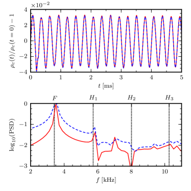
Note that the star is essentially opaque to neutrinos as the neutrinosphere is located very close to the star surface. Furthermore, because the diffusive neutrino emission is expected to take place on a diffusion time scale, s, that is much longer than the dynamical time scale, ms, we expect that the star will cool only very slowly. Most of the emitted neutrinos, in fact, will be reabsorbed in the hot central region. As a result, the net luminosity will predominantly be produced by the outer stellar layers, where the neutrinosphere is located, and will be modulated following the smooth harmonic oscillations introduced by the perturbation. In general the different neutrinospheres are located in a shell of km near the stellar surface, with the electron-antineutrinos neutrinosphere being located deeper inside the star when compared to the other neutrinos species (cf., Fig. 14).
In the top panel of Fig. 4, we plot the evolution of the normalized central rest-mass density for the model evolved without neutrino emission (blue dashed line) and with the NLS (red solid line). Note that the neutrino emission has a negligible effect on the evolution of the bulk motion of the star. Only at late times, the two evolutions start to show very small differences that can be hardly noticed in the figure unless it is magnified. The lower panel of Fig. 4 shows the PSDs of the central rest-mass density for the two evolutions and compares them with the predictions (vertical black dashed lines) from a linear-perturbation code for the same models. Overall, the agreement between the linear and nonlinear codes is rather good, with a difference of in the frequency of the -mode. As for the case of the radial pulsations of cold stars in Sec. VI.1, we note the presence of modes that are not predicted by the linear theory. Once again, we associate the peak around to nonlinear couplings as it is located at exactly twice the frequency of the -mode. Finally, we note that the frequencies for hot stellar models differ only slightly from the corresponding values obtained for zero-temperature models with identical baryon mass. In this case, the difference is only in the -mode frequency and increases to for the -mode.
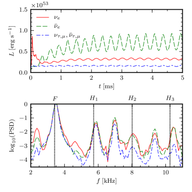
As anticipated, the harmonic time dependence of the fluid variables is reflected also in the neutrino luminosities, which we compute according to Eq. (69) with .
The evolution of the luminosity is shown in the top panel of Fig. 5, with different lines referring to different neutrino species. Overall, it does not come as a surprise that the modulation of the neutrino luminosities for the different species reflects the oscillation frequencies of the star as shown in the PSDs reported in the lower panel of Fig. 5. Note however that electron-neutrinos and heavy neutrinos show smaller-amplitude oscillations in the luminosity than the electron-antineutrinos. This is probably related to the relative position of the corresponding neutrinospheres with respect the node of the eigenfunction of the fundamental mode. In particular the electron-antineutrinos neutrinosphere is located deeper inside the star compared to the other species.
We note that the local luminosity in Fig. 5 is effectively different from the one that would be measured by a distant observer. First, the modulation would be smaller than that in Fig. 5; this is because sums up all the neutrinos emitted at a given coordinate time, which however do not reach the observer at the same time. As a result, the signal would resemble a running average of the luminosity over a time interval given by the light-crossing time, which is of the order for a NS. Second, the luminosity would also be reduced by a factor because of the gravitational redshift. Finally, because part of the neutrinos emitted inward would be absorbed by the NS core, the luminosity would be further reduced by a factor up to .
Even though the total evolution time is not sufficiently long to clearly see the effects of the neutrino cooling on the lower order modes, there are small differences between the eigenfrequencies when comparing to a cold NS with identical baryon mass. For a star cooling down over longer time scales, we expect an impact mainly on the higher-order modes. This can be explained simply in terms of the nodal points of the corresponding eigenfunctions, which are located closer to the surface in the case of higher-order modes. As a result, they are affected more strongly by the changes in composition taking place near the surface.
VI.3 Hot stars: Migration or collapse to black hole
Another important test for the correct implementation of the NLS is represented by a classical benchmark in relativistic-hydrodynamics codes: the dynamics of a nonrotating relativistic star on the unstable branch of the configurations of equilibrium. This test, which was first considered in three dimensions in Refs. Baiotti et al. (2005b); Font et al. (2002), involves the evolution of equilibrium models that are unstable to the fundamental quasiradial mode and which, upon the introduction of a perturbation, will either increase their central rest-mass densities and collapse to a BH, or decrease their central rest-mass densities and hence migrate to a new configuration on the stable branch of equilibria. We note that this process can also exhibit a critical behavior Liebling et al. (2010); Radice et al. (2010), which however we will not consider here. Both evolutionary paths are equally probable and in both cases the stellar models are expected to maintain the same baryonic mass. The degeneracy between the two possible evolutions is therefore broken by the properties of the initial perturbation. In view of this we introduce a well-defined velocity perturbation instead of leaving the growth of the dynamical instability to the cumulative effect of the numerical truncation error, since this might depend on the grid resolution, reconstruction technique, symmetries and other details of the evolution scheme. The perturbation consists of a simple radial velocity profile with positive or negative sign in order to trigger either the migration to the stable branch or the collapse to BH.
We consider three initial TOV models for this test, where the first two are constructed assuming -equilibrium and a constant entropy distribution of for both the LS-EOS and SHT-EOS (i.e., uTOV-LS and uTOV-SHT). The third model uses the SHT-EOS and has a constant temperature of (i.e., uTOVh-SHT). The last three rows of Table 2 report the properties of the different models along with the maximum mass models for the two EOSs. Note that all the models have a central rest-mass density that is larger than the central rest-mass density of the model with the maximum mass. The temperature profile for these stars reaches at the center for the LS-EOS and for the SHT-EOS, while for both EOSs the surface temperature is around . Hereafter we will concentrate only on models, uTOV-LS and uTOV-SHT, while model uTOVh-SHT will be used to show our convergence properties in Appendix B .
During the collapse to a BH, the central rest-mass density will increases, inevitably exceeding the upper limit of the EOS tables. For the purpose of this code test, we extended the EOSs to higher densities by the following prescription. First, we extend the EOS at zero temperature to higher densities by assuming that the pressure stays constant. Thermodynamic consistency then yields the specific energy at zero temperature. For higher temperatures, we use a zero-order extrapolation of the pressure along lines of constant . Of course, the prescription at higher densities will have an influence on the speed of the collapse as soon as those densities are reached. However, the purpose of the extension is not physical realism, but testing the ability of the code to follow the collapse and BH formation.
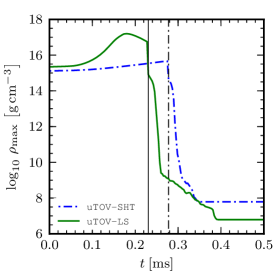
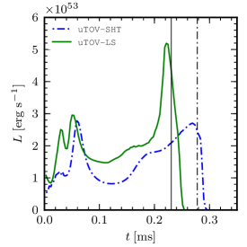
When driven by a negative radial velocity perturbation, all models evolve towards a gravitational collapse. We follow the evolution of the collapsing matter until the formation of a BH when an apparent horizon is detected. The results of these collapsing simulations are shown in Fig. 6, where the left panel displays the evolution of the maximum rest-mass density for both the extended SHT-EOS (blue solid line) and the extended LS-EOS (green solid line), normalized to the initial value. Note the central density exceeds the range of the EOS tables during collapse (for the LS-EOS the overshooting is of more than one decade). We also note that after , the density profile develops a pronounced peak near the center, which is numerically under-resolved. We assume that this affects mainly the central region and not the outer layers, which are still falling in. Because of these two reasons, the decrease in central rest-mass density observed for the LS-EOS at ms is likely an artifact. The luminosity, however, should not be influenced by this since it is mostly produced in the outer layers of the collapsing star. For both models, the time of the collapse is of the order of a few tenths of a millisecond before an apparent horizon is detected (marked with a vertical solid or dashed line).
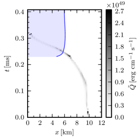
We also computed the neutrino luminosity according to Eq. (69), using and excluding the interior of the apparent horizon from the integral. The result is shown in the middle panel of Fig. 6. For the models uTOV-LS, and uTOV-SHT, we find that the emitting region is a very thin shell close to the surface, resolved by only a few grid points. This is shown in the right panel, which represents a spacetime diagram of the local emissivity for model uTOV-LS; note that most of the contribution to the luminosity takes place from a thin shell away from the apparent horizon (blue solid line). Such models represent an extremely challenging test for the NLS and the corresponding luminosities should therefore be taken with care. For the constant-temperature model uTOVh-SHT however, the emitting region is much larger and well resolved (see Appendix B).
Soon after an apparent horizon is formed, it covers most of the emitting material and indeed the neutrino signal terminates abruptly. As noted in Sec. VI.2, we should again stress that the luminosity we compute here is not necessarily a good approximation for the luminosity seen at infinity once the emitting shell comes close to the horizon. Already for the simpler case of a stationary BH, our assumption that all neutrinos reach infinity is less accurate than for a NS. This is because the neutrino luminosity seen by our coordinate observer is divided unevenly between highly redshifted outward-moving neutrinos and blueshifted inward-moving neutrinos which fall into the BH. Thus, Eq. (69) does not reproduce the very high redshift seen by a distant observer of the infalling matter close to the horizon. Another effect not taken into account is that neutrinos emitted closer to the horizon also need more time to reach a distant observer, while the luminosity we compute is a function of the coordinate time of the emission. Finally, estimating the signal that would observed at infinity is made even more difficult by the nonstationarity of the spacetime. For these reasons, we only reported the luminosity at the source, using . We have checked, however, that most of the energy is always emitted at reasonable distances from the horizon (see again the right panel of Fig. 6).
We now turn to discussing the dynamics of model mTOV-SHT, which is perturbed with a positive radial velocity in order to trigger a migration to the stable branch. The top panel of Fig. 7 displays the evolution of the central rest-mass density, while the bottom panel shows the evolution of the three different luminosities. As expected, the introduction of the perturbation triggers a very rapid expansion of the star, followed by a series of oscillations as the star tries to attain a new equilibrium on the stable branch of configurations. Because the new equilibrium configuration has the same baryonic mass but a smaller gravitational mass, the energy difference is simply transformed into kinetic energy and dissipated in part by shock heating at the stellar surface, which in turn leads to neutrino emissions. Note that the evolution of the oscillation amplitude shows a strong damping due to shock formation Radice and Rezzolla (2011); Kastaun (2011). This behavior resembles closely the one found for an ideal-gas EOS as discussed, for instance, in Refs. Font et al. (2002); Cordero-Carrión et al. (2009).
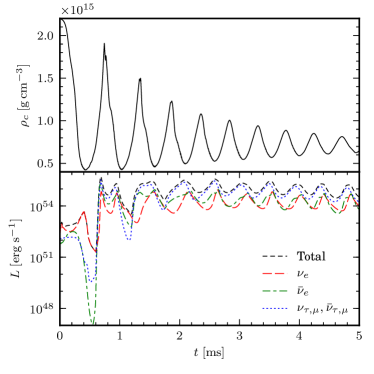
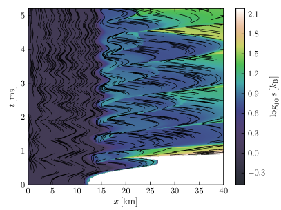
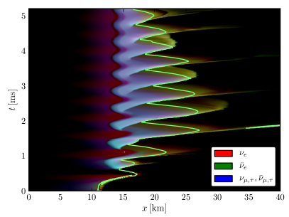
Particularly interesting is the evolution of the neutrino luminosity that accompanies the various phases of expansion and contraction. We studied the time evolution of entropy, neutrino emissivities, temperature, and opacities along the -axis. The first two are shown in Fig. 8, from which we find that the total luminosity is the result of several different effects. We can divide the emitting region into an inner one, at radii between –, where the star oscillates nonlinearly, but without significant shock formation, and an outer region, extending to , where low density matter is heated up to by shock formation. Those shocks are caused by material from the outer layer that is expanding very far and then falls back, colliding with denser regions which are already expanding again. Those shocks are present at each oscillation. The neutrino luminosity from the inner region is determined by the balance between two effects. First, the temperature decreases when the star expands, lowering the local emission rates. Second, the optical depth decreases when the star expands, thus enhancing the effective emission rates. For our setup, the latter effect is stronger, such that the luminosity is largest when the star is expanded. The behavior of the inner region is similar to what we expect for a linear oscillation of a stable star, and explains the modulation of luminosity in Fig. 5. The luminosity in the outer layers on the other hand follows essentially the temperature evolution due to the shock heating, while the optical depth is irrelevant since the densities are low. At radii between roughly – both heavy neutrinos and electron-antineutrinos are emitted, while at radii larger than mostly electron-antineutrinos are emitted. Note the intermediate regime between free emission and pure diffusion is more extended than for a stationary NS, and the position of the neutrinosphere, shown in Fig. 8 with a bright green solid line, just serves to approximately distinguish the two regimes (there can be multiple locations for the neutrinosphere at the same time, referring to different emitting regions). The initial dip in the luminosities is due to a pronounced peak in the opacity at roughly , which vanishes later when the material is heated. The nature of that peak has yet to be identified. We also note that during the first 0.5 ms, when the surface expands rapidly into the artificial atmosphere, the luminosity may be influenced by treatment of the atmosphere.
The tests discussed in this section, although very idealized, provide us with a well-controlled environment in which to understand the relationship between the matter dynamics and the neutrino emission. The understanding of the matter-radiation interaction within the NLS gained in such simplified settings may help to understand the neutrino signals from more complicated scenarios, such as BNS mergers Sekiguchi et al. (2011a, b).
VII Applications of the NLS: neutrino-induced collapse
After having discussed the ability of our code to properly account for the neutrino emission from isolated NSs within the NLS, we next consider the application of the code to explore novel aspects of the dynamics of these objects and in particular the conditions under which neutrino radiative losses can induce the collapse to a BH. More specifically, we will present the results of simulations of hot nonrotating NS models close to the maximum mass and show that the combined effects of neutrino cooling and deleptonization can drive a stable model to collapse gravitationally to a BH. Conversely, when these effects are neglected, the evolution leads to a stable star oscillating in its eigenmodes. Although this is an interesting scenario that has not been investigated before in consistent three-dimensional simulations, we should also remark that for NSs with temperatures close to the ones reached by the PNS in numerical simulations of stellar-core collapse or by the HMNS in the case of BNS mergers, the instability discussed here can be triggered only in an extremely narrow range of masses near the maximum one. Similar results are also reported in the study of equilibrium models of rotating hot NS Hashimoto et al. (1994) and more recently for HMNS Kaplan et al. (2013).
VII.1 Considerations from equilibrium models
Before discussing in detail the results of the dynamical simulations, it is instructive to make a number of considerations based on the properties of equilibrium models and on quasistationary transformations along sequences of equilibrium. We will then realize that the process of cooling of a stable relativistic star which conserves baryon mass is far less obvious than may appear at first sight and that it is actually very difficult to make any reliable prediction about what is the outcome of this process.
Suppose here that we wish to represent the evolution of a cooling NS through a sequence of quasistationary nonrotating equilibrium configurations. To restrict the range of possibilities we need to make the following assumptions: (i) the star model moves through a series of equilibria during the cooling process, keeping its baryonic mass constant; (ii) the cooling process is sufficiently slow compared to the time scale of the processes, so that -equilibrium can be considered to be maintained at all times; (iii) the temperature profile in the star is either isentropic (i.e., the entropy per baryon is constant inside the star), or isothermal (i.e., the temperature is constant inside the star); (iv) the gravitational mass is reduced by the neutrino losses.
Having made these assumptions, we can study the outcome of the cooling process by comparing the gravitational and baryonic masses of TOV sequences in -equilibrium with different temperatures (this idea was already explored in Ref. Ibanez Cabanell (1981) in a more simplified EOS). To this scope we have constructed isothermal or isentropic sequences of nonrotating TOV solutions, shown in Fig. 9. We first concentrate on the isentropic case, to come back to the isothermal one later on.
For an isentropic sequence with a given specific entropy, there is one stellar model which maximizes both the gravitational mass and the baryon mass . We recall that the criterion of stability against radial perturbations for a spherical relativistic star states that a configuration with a central rest-mass density larger than the one of the model with the maximum gravitational mass is unstable with respect to radial oscillations Harrison et al. (1965); Ipser (1970). This criterion, which is also known as the ”turning-point” criterion Friedman et al. (1988), has been verified in a number of simulations, for instance Gondek et al. (1997); Goussard et al. (1998); Baiotti et al. (2005a); Baiotti and Rezzolla (2006), and represents a reasonable first approximation also in the case of rotating stars Takami et al. (2011)222We also remark that for rotating stars, the turning-point criterion is only a sufficient condition for secular instability and not a necessary condition for secular and dynamical instability. Hence, a stellar model which is stable according to the turning-point criterion, can be nevertheless dynamical unstable, as shown by Takami et al. (2011) through dynamical simulations.. Hence a NS model with divides the sequence into a stable branch and an unstable branch; models on the unstable branch are unstable to radial perturbations, which cause the stars to either collapse to a BH or to expand and oscillate around a distinct and stable equilibrium configuration, as discussed in the previous Section.
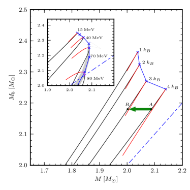
The question is now whether it is possible to move continuously along equilibrium configurations belonging to sequences with decreasing specific entropy, while decreasing the gravitational mass and conserving the baryon mass. To answer this, we plot a number of sequences in a diagram, as shown in Fig. 9 for the specific example of the LS-EOS. The green arrow indicates a cooling process satisfying our conditions and connecting two putative starting and ending states and , both on the stable branches of equilibrium configurations.
Note that in general the maximum baryonic mass decreases with increasing entropy and, as one would expect for a star losing energy via radiation, that the gravitational mass decreases along sequences with decreasing entropy. For example, a model with a baryonic mass of will radiate about of its gravitational mass when going from an isentropic configuration with to one with zero temperature. We thus find that the idealized cooling process through stable equilibrium models is not prohibited by energy or mass conservation.
However, a careful look at the figure will reveal that the trajectory from to also intersects the unstable branches. This raises the question if it is possible for a model on the stable branch to change into a model which has identical baryon mass and gravitational mass, but lies on the unstable branch of another sequence. When only considering energy and mass conservation, there is nothing that would prevent such a transition. It would however require a finite, discontinuous reduction of the stellar radius. Since we allow only for transformations that reduce the gravitational mass, also the specific entropy has to be reduced by a finite amount when transitioning to an unstable branch, e.g., as a result of a phase transition Abdikamalov et al. (2009), as can be seen from Fig. 9. Assuming that the star does not change its radius discontinuously, a transition to the unstable branch cannot happen through a sequence of isentropic equilibrium models. It would however be difficult to prove conclusively that no such transition is possible through any conceivable dynamical process or through nonisentropic equilibrium models, e.g. when cooling first the outer layers and then the core. This question is not to be confused with the usual stability analysis, which describes adiabatic perturbations.
In any case, whether or not the above crossings to unstable branches could happen in nature cannot be decided from the idealized cooling model, but requires a fully dynamical description. This is particularly relevant for models approaching the maximum mass, where the jumps in radius and central density between stable and unstable models become arbitrary small and can be more easily overcome by finite perturbations. Let us therefore consider possible trajectories in parameter space when allowing the above transitions between stable and unstable models, but still restricting ourselves to isentropic models for simplicity. This is illustrated in Fig. 10, which shows the gravitational masses and radii along three isentropic sequences with and . Also here we have marked the two states and and shown with a solid green arrow the simplest of the possible trajectories, namely, one leading from to across models on stable branches. Alternatively, the star could cool down along stable equilibrium sequences, then cross over to an unstable branch via some hypothetical process, reducing the radius and the specific entropy, but conserving baryonic and gravitational mass. It could then continue to cool down along unstable equilibrium sequences. Such a process is summarized by the green dashed arrow, connecting model to a model on the unstable branch with . Once on the unstable branch, the star can either collapse to a BH (moving further to the left) or ”migrate” back to the stable branch (green dotted arrow), following the dynamic instability discussed in the previous Section. In doing so it will expand, going from a radius of, say, km to km and further cool (note that the gravitational mass decreases). Once on the stable branch, it can further cool and go to state or move again to the unstable branch of the sequence with , where the same considerations made above can be repeated.
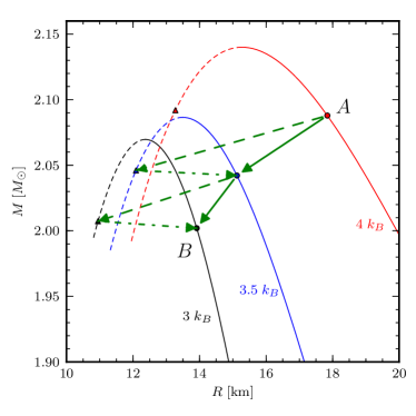
As anticipated above and as shown rather clearly in Fig. 10, considering equilibrium sequences and energy arguments does not allow us to reach any firm conclusion on the fate of a relativistic star that cools via radiative losses. It may seem reasonable to expect that the transition involving only states on the stable branches is favored as in this case the star undergoes the minimal changes in radius and density, without abrupt contractions and expansions. However, no energetic argument can really be used in support of this conjecture.
We now return to the question of what happens under the assumption of isothermal cooling. The corresponding equilibrium sequences are depicted in the inset of Fig. 9. Also here, the maximum baryonic mass is decreasing with increasing temperature. Note however that in this case the maximum gravitational mass is not anymore monotonically increasing with temperature. In fact, at temperatures above the maximum mass decreases with increasing temperatures as larger and larger portions of the star become dominated by the pressure support of photons and electrons. Also note that for the highest temperature models we even find that , i.e., one would gain energy by dispersing the stellar matter to infinity. Another intriguing property of the isothermal solutions is that maximum gravitational and maximum baryonic mass are not reached at the same central rest-mass density. As shown by Refs. Gondek et al. (1997); Gourgoulhon and Haensel (1993), the turning-point criterion needs to be extended under these conditions, although we still regard it as a good estimate. Although in Fig. 9 we have employed the LS-EOS, very similar qualitative results are obtained when using the SHT-EOS. Finally, it is not yet clear whether the region with can really be considered to represent realistic models and is not instead just an artifact of the EOSs for very large temperatures. What is clear, however, is that the relation between temperature, entropy and gravitational mass becomes more complicated when thermal effects are considered as these can change significantly the rest-mass density profile.
In summary, we have shown that no conclusive predictions can be made on the evolution of a cooling relativistic star on the basis of equilibrium considerations. This represents a perfect motivation to make use of fully numerical simulations which can shed light on this process and account, for instance, for the fact that cooling processes are far from being homogeneous throughout the star. The outer layers of the hot NS would cool down much faster than the core, creating an entropy or a temperature gradient that might lead to the formation of convective cells or the contraction of the outer stellar layers. This is indeed the focus of the following Sec..
VII.2 Dynamical simulations of neutrino-induced collapse
Having constructed equilibrium models of hot NSs, we now address the question of how the stability of a nonrotating relativistic star against radial perturbations is affected by changes in temperature and composition. It is important to remark that the turning-point criterion was obtained under the simplified assumptions that the radial perturbations conserve entropy and that the chemical equilibrium is reached essentially instantaneously (or on time scales much smaller than those of the radial oscillation), such that the composition is always the one at -equilibrium. If this last condition is not satisfied, and instead the time scale of the weak-interaction process is longer than (or comparable to) the oscillation time scale, then the composition of the initial configuration is simply advected along with the fluid elements Chanmugam (1977); Gourgoulhon and Haensel (1993). As a result, for central rest-mass densities near that of the maximum-mass model, i.e., near , where the oscillation period of the fundamental radial mode tends to diverge and where infinitesimal perturbation might destabilize the configuration, the time scale of the changes in composition could have an important dynamical effect (this was pointed out already by Ref. Gourgoulhon et al. (1995)). Clearly, the only way to assess the stability properties under conditions in which the effects of weak processes are taken into account and can be influential, is by performing the fully nonlinear numerical simulations that we report below.
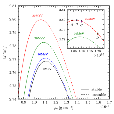
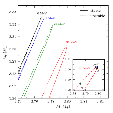
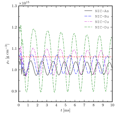
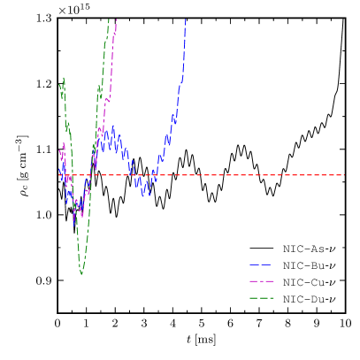
We have therefore selected a sequence of NS models with in -equilibrium close to the maximum gravitational mass allowed by the SHT-EOS. The reason behind this choice is that the results of the linear stability analysis of hot PNS models performed by Ref. Gondek et al. (1997) have shown that the impact of temperature and composition on the radial eigenfunctions is stronger for isothermal configurations. The properties of our models, named NIC-As to NIC-Du, are listed in Table 3.
These models are also shown on a diagram in the left panel of Fig. 11 as models –. For each sequence we distinguish with solid and dashed lines models that are on the stable and unstable branches, respectively. The right panel of Fig. 11 shows the same sequences in a diagram. Note that the influence that the temperature has on the maximum mass is only very small (as mentioned already, the pressure shows only a very weak dependence on temperature near nuclear densities; cf., left panel of Fig. 1). The maximum mass of the cold model (i.e., ) is only smaller than the one of the hottest model at (cf., right panel of Fig. 11). A closer comparison between these two models is offered in Table 3, where they are denoted as MAX-0 and MAX-30, respectively.
| Model | |||||||
|---|---|---|---|---|---|---|---|
| MAX-0 | 13.31 | ||||||
| MAX-30 | 17.40 | ||||||
| NIC-As | 17.66 | ||||||
| NIC-Bu | 17.45 | ||||||
| NIC-Cu | 17.26 | ||||||
| NIC-Du | 16.72 |
Resolving the minuscule differences between these models in numerical simulations is quite challenging, also in terms of the computational costs. Our simulations make use of three fixed nested refinement grids centered on the NS, with a resolution of the finest grid of (i.e., points across the star). The extent of the finest grid is large enough to include the entire star and the outermost boundary is located at a distance of . The spherical grid used to compute the optical depth has a radial resolution of , 100 points in the -direction, and 50 along the -direction. Also in this case we set the density of the artificial atmosphere to the lowest value available in the SHT-EOS table (i.e., ).
The results of these simulations are collected in Fig. 12. The left panel depicts the evolution of the central rest-mass density when the neutrino radiative losses are not taken into account. The different lines refer to the four different models. As a reference, the horizontal dashed line marks the central rest-mass density of the maximum-mass model, . Note that no perturbation was introduced in the initial data and the oscillations are triggered simply by the truncation error.
As expected in the absence of neutrino losses, model NIC-As, which is on the stable branch, simply oscillates in its fundamental mode with an amplitude that is larger when compared to the simulations using Cowling approximation studied in Sec. VI.1. The corresponding frequency is of the order of , in good agreement with what was found in Ref. Takami et al. (2011) when computing the neutral-stability line in relativistic stars. Interestingly, models NIC-Bu, NIC-Cu and NIC-Du, which are instead on the unstable branch, migrate on a dynamical time scale to the stable branch, expanding and reducing their central rest-mass density while conserving baryonic mass. Once on the stable branch they simply oscillate with amplitudes which are large but with the central rest-mass density remaining below the initial one [just compare with for models NIC-Bu–NIC-Du], but with excursions that go above above (only model NIC-As has oscillations that remain below ).
In all of these simulations, there is no significant mass loss neither from the outer boundary or from the treatment of the atmosphere surrounding the star. The conclusion to be drawn from the left panel of Fig. 12 is therefore that, in the absence of neutrino losses, none of the models considered collapses to a BH. Furthermore, even models that are initially unstable, simply migrate to the stable branch. We note however that the perturbations required as a trigger are given by discretization errors, and a collapse to a BH seems equally possible.
The dynamics of these same models is very different if the neutrino losses are taken into account. This is shown in the right panel of Fig. 12 and it is straightforward to realize that all the models are now dynamically unstable over time scales of –. Let us first analyze the unstable models NIC-Bu, NIC-Cu and NIC-Du. Overall, the cooling produced by the neutrino losses, which is already active after about (cf., Fig. 15) induces a perturbation that leads to the final gravitational collapse. However, before collapsing to a BH, all of the unstable models actually expand until the central density is well below the one of the maximum-mass model, just as they did in the absence of neutrino losses (compare the same lines in the left and right panels of Fig. 12). The continuous radiative losses experienced by these models and the corresponding pressure depletion, however, are such that these models progressively collapse to a BH. Not surprisingly, the first model to collapse is the one that was originally further away from the maximum central density, i.e., NIC-Du, and that is also subject to the largest oscillations. Similarly, the duration until collapse of the other unstable models is progressively longer, the closer they are to the maximum-mass model. Before collapsing, each model loses a significant fraction of the total thermal energy stored in the initial configuration. The radiated energy can be as high as 0.4% of the initial mass (see Table 3 for details).
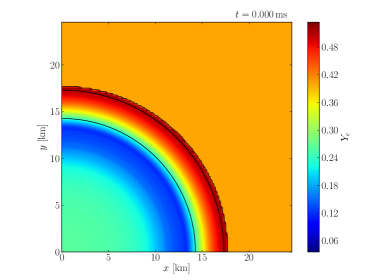
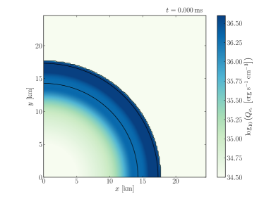
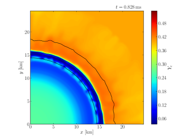
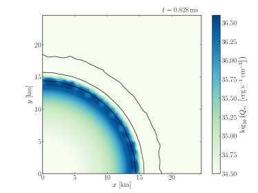
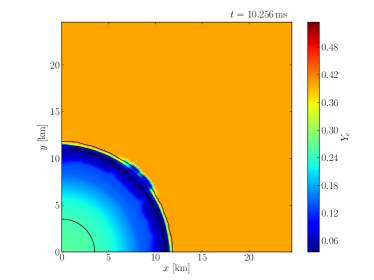
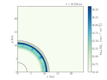
Note that the oscillations of all models in the right panel of Fig. 12 show the presence of the fundamental mode with frequencies of the order of , but also of the first overtone with frequencies around . This mode is excited mostly in the outer layers of the star by the rapid expansion and rarefaction driven by the neutrino emission and is therefore strongly imprinted in the neutrino luminosities (cf., Fig. 15). A similar behavior has been reported already in the calculations discussed in Ref. Gourgoulhon et al. (1995).
On a much longer time scale of , but following a similar dynamics, also the stable model NIC-As encounters the gravitational instability, and the dynamical collapse to a BH begins. In this case, a secular increase of the central rest-mass density is clearly visible that was of course not present in the absence of neutrino losses. This secular increase is due to the combined effects of a slow deleptonization and to the cooling of the outer layers of the star close to the neutrinosphere, which lead the star to cross the stability limit in rest-mass density, (shown as red dashed line).
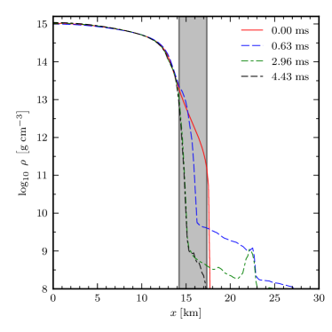
Additional information on the dynamics of the stable model NIC-As is presented in Fig. 13. The left panels show the electron fraction at representative times on the plane, while the right panels show the electron-neutrino emissivity. In all panels we also plot isodensity contours, with the outermost one marking the position of the stellar surface (i.e., the position of the first fluid elements at density equal to the that of the atmosphere). Note the very rapid deleptonization caused by the neutrino losses, which reduce the electron fraction in the outer layers of the star to values . Note also that the rapid cooling of the outer envelope of the star leads to a net reduction of the stellar radius, which decreases from down to (cf., the second outermost contour line marking of the initial central rest-mass density). This effective radius also coincides with the location of the maximum electron-neutrino emission at all times during the simulation (cf., right panels).
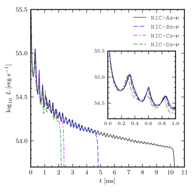
Another interesting aspect that emerges from Fig. 13 is the appearance of a convective layer at a radius around (cf., the middle row of panels). We recall that a convective instability is expected to develop if the Ledoux criterion Ledoux (1947); Epstein (1979) is satisfied, i.e., if
| (72) |
Using this criterion we find that the radius at which becomes positive is approximately , which is where in fact the first eddies appear in our simulations (this result indeed applies to all of our models in this Sec.). The unstable region is located around the neutrinospheres and the convection actively enhances the deleptonization, contributing to an increase in the neutrino luminosity and consequently to the cooling of the hot outer envelope Keil et al. (1996). During the evolution, the convective layer moves inwards until it reaches the neutrinosphere. The neutrino-opaque interior, however, is not affected by convection, at least over the time scale of our simulations and thus no significant changes in the composition of the core are measured (cf., the bottom row of panels). Finally, we note that the slight asymmetry that can be detected along the diagonal on the last panels of Fig. 13 is simply due to the use of Cartesian coordinates and converges away with resolution.
A more careful look at the deleptonization occurring in the stellar envelope and the corresponding neutrino losses can be made by analyzing the rest-mass density profile for the stable model NIC-As. This is shown in Fig. 14, where different lines refer to different times in the evolution. Note how the outer envelope of the star, sustained by the lepton pressure, undergoes a rapid cooling leaving exposed the hot stellar interior. The neutrinosphere also shrinks, following the motion of the stellar surface. Outside the neutrinosphere the effective emission rates given by Eqs. (61)–(62) are dominated by the free emission, thus leading to a rapid release of energy. This initial burst in neutrino emission can also be clearly seen in Fig. 15, which reports the evolution of the total neutrino luminosity for the models described in Table 3, and where the total neutrino luminosity reaches values over erg s-1 for all of the models considered. As the external envelope is cooled down, it contracts, thus contributing to the secular increase in central rest-mass density discussed in Fig. 12. The cooling is effective at all times and the stars continue to emit neutrinos with a luminosity that has decreased by about 1 order of magnitude over for the long-lasting model NIC-As. Once again we remark that most of this emission is produced in the outer layers of the star since the interior is mostly optically thick.
In summary, the simulations reported in this Sec. provide convincing evidence that stellar configurations near the maximum mass of nonrotating stellar models can be induced to collapse to a BH if subject to radiative losses. The very same models that collapse do not show any sign of instability in the absence of radiative losses and even models that are metastable (i.e., on the unstable branch) can migrate to the stable branch, where they oscillate stably with large amplitude. Although rather idealized (we are considering only spherical stars under very controlled conditions), this result has an impact also on those studies concerned with the formation of a PNS in simulations of stellar-core collapse or of a HMNS in the case of BNS mergers. While in fact we provide evidence that neutrino-induced collapse of stars near the stability threshold is indeed possible, as already suggested in Ref. Paschalidis et al. (2012), our results also indicate that this process is more delicate than it may appear at first sight, being possibly restricted to a small portion of the space of parameters.
VIII Discussion and conclusions
We have presented the implementation in the Whisky code of a new scheme to describe the evolution of nuclear matter by means of a microphysical finite-temperature EOSs and by a simplified neutrino leakage scheme (NLS) to account for radiative losses via neutrinos and the corresponding changes in composition. Although this is not the first time that a NLS is employed in numerical simulations, even in general relativity, we have tried to provide ample and pedagogic details about our implementation, including a detailed description of a novel and robust technique for the transformation from conserved to primitive variables to be used with tabulated EOSs. We expect that this information will be of help for anyone wanting to reproduce our results or wishing to implement a NLS in a general-relativistic-hydrodynamical code.
Using the new code we have carried out an extensive investigation of the properties and limitations of the NLS for isolated relativistic stars to a level of detail that, to the best of our knowledge, has not been discussed before in a general-relativistic context. In particular, we have presented a series of tests on linear and nonlinear oscillations of cold and hot NSs, which have given us the possibility to test the code against the predictions of the linear-perturbation theory. Overall, we have demonstrated the ability of the code to account for the neutrino emission from an isolated neutron star within the approximation of the NLS and to capture, at least as a first approximation, the radiative losses and the rapid changes taking place in the matter properties.
In addition, we have explored some novel aspects of the dynamics of hot, isolated NSs and, in particular, the conditions under which neutrino radiative losses can induce their collapse to a BH. These conditions cannot be assessed conclusively using considerations on quasistationary transitions across equilibrium models, but rather need the use of fully nonlinear and self-consistent numerical simulations.
More specifically, using the newly developed code we have presented the results of simulations of hot nonrotating NS models close to the maximum mass and shown that the combined effects of neutrino cooling and deleptonization can drive a stable model to collapse gravitationally to a BH, thus confirming previous results obtained with 1D calculations Gourgoulhon et al. (1995). On the other hand, we have also shown that radiative losses are neglected, the evolution leads to stable stars oscillating in their eigenmodes. Although this scenario has not been investigated before in three-dimensional simulations, it really applies only to NSs with very high temperatures close to those reached by PNSs or HMNSs, with the instability being triggered only in an extremely narrow range of masses near the maximum one.
The numerous tests considered here are admittedly idealized, but they provide a well-controlled environment in which to understand the relationship between the matter dynamics and the neutrino emission, which is of course important to understand the neutrino signals from more complicated scenarios, such as BNS mergers, and which will represent the future application of our code.
Acknowledgements.
We thank D. Radice, C. D. Ott, Y. Eriguchi, I. Hinder, M. Obergaulinger, G. Shen, P. Cerdá-Durán and N. de Brye, for useful discussions and comments. A special thank goes to José María Ibáñez, for his initial work on the stability of hot stellar models and for the numerous discussions on this topic. This work has also benefited from the stimulating atmosphere of the MICRA workshop in 2011. We also thank Aaryn Tonita for the essential support and collaboration in the development of the code. Finally, we are also grateful to the anonymous referee for the thorough and helpful report. The numerical computations were performed on the supercomputing cluster at the AEI. This work has been partially supported by the ”Compstar”, a Research Networking Programme of the European Science Foundation. Partial support also comes from the VESF Grant (EGO-DIR-69-2010) and the DFG Grant SFB/Transregio 7. JAF also acknowledges support by the Spanish MICINN (AYA 2010-21097-C03-01) and by the Generalitat Valenciana (PROMETEO-2009-103).Appendix A Neutrino free emission rates and opacity sources
In this appendix we will review the various weak-interaction processes with the NS matter at different densities, temperatures and compositions. Our primary goal is to obtain the expressions for the neutrino emissivity, (energy emitted via neutrinos per second and baryon) and the neutrino emission number rate, (number of neutrinos emitted per second and baryon). These explicit expression are used in Sec. III to compute the effective source terms accounting for neutrino radiation in the hydrodynamic evolution equations. We should note that all of the material presented here can be found, although dispersed, in several other publications, e.g., Ruffert et al. (1996, 1997); Ruffert and Janka (1999, 2001); Rosswog and Davies (2003); Rosswog and Liebendörfer (2003); Rosswog et al. (2003); Wilson and Mathews (2003), and that our goal here is mostly that of providing a single-point reference for these expressions.
We start by recalling that there is a variety of neutrino emission mechanisms that are important at different densities and temperatures within the NS matter. The most important of those mechanisms are: (i) electron and positron capture on nucleons ( process); (ii) electron-positron pair annihilation; (iii) transverse plasmon decay.
The emission rates corresponding to the three mechanisms above can be approximated through simple analytical formulas that depend only on quantities provided by the EOS tables. We start from the simplest and most powerful neutrino emission from hot and dense nuclear matter, the direct Urca process. It consists of two reactions, the -decay and the electron capture on free nucleons ():
| (73) |
This is the process that drives the nucleons toward the -equilibrium where the chemical potentials of the electron neutrino and antineutrino are zero, , and the rates of both reactions are the same, leaving the composition of the matter unchanged. The neutrino emissivity and the neutrino emission number rates for the -decay are given respectively by the following expressions Bruenn (1985)
| (74) | |||
| (75) |
For the electron capture they are similarly defined as
| (76) | ||||
| (77) |
where is the blocking factor for a neutrino Fermi-Dirac distribution, , and is a constant defined as
| (78) |
where , the weak axial-vector coupling constant is , and are the degeneracy parameters for the different particle species. Temperatures are always expressed in units of energy.
The occupation probability of electrons, positrons, neutrinos, nucleons and nuclei follows the relativistic Fermi-Dirac distribution with a temperature equal to that of the fluid. The relativistic Fermi integrals of order are defined as
| (79) |
and they depend on the value of the relativistic chemical potential, , for each different fermion species. The evaluation of the Fermi integrals cannot be done analytically. Although the numerical integration is relatively straightforward, it is convenient to use an approximate analytic solution as suggested in Takahashi et al. (1978). After the interaction with the electron (positron), the phase space of the degenerate proton (neutron) is reduced by the Pauli blocking factor, , given by
| (80) |
where and are the neutron and proton number density and is the difference between neutron and proton relativistic degeneracy parameters. In regions where and , and where the fraction of free nucleons is small but not zero, the Eq. (80) can lead to nonphysical values of the blocking factors. We simply approximate the Eq. (80) in the nondegenerate regime (for densities below ), with .
Finally, the lepton phasespace is reduced by the Pauli principle, which is taken into account by the approximate expressions
In low density and high temperature nondegenerate nuclear matter, annihilation of electron-positron pairs is an extremely efficient neutrino mechanism
| (83) | |||
| (84) |
This process can be accurately calculated from temperature and electron fraction of the matter (see (Itoh et al., 1996) and for a review on the topic see (Yakovlev et al., 2001)) by the following formula for the emission number rates for electron-neutrino and antineutrino
| (85) |
where is the electron mass, and are given in terms of the normalized vector () and axial constants ()
| (86) |
For convenience we define the energy moments of the Fermi-Dirac distribution for massive particles (electrons and positrons) as
| (87) |
where is an integer number. The neutrino emission rate due to pair annihilation, for the heavy neutrinos and (and for the respective antiparticles), is given by
| (88) |
with , and with the phasespace blocking factor for the different neutrino species approximated as in Cooperstein et al. (1986, 1987) by
| (89) |
The neutrino emissivities due to electron-positron annihilation for the different neutrino species are
| (90) |
At medium densities and high temperatures, one of the major sources of neutrino emission comes from plasmon decay. We recall that plasmons are quanta of electromagnetic field in a plasma and they can appear with two distinct polarizations, longitudinal and transverse. In the regime of our simulations, the longitudinal polarization can be neglected (Schinder et al., 1987; Kantor and Gusakov, 2007), and the plasmon decay can be written as
| (91) | |||
| (92) |
where stands for a plasmon and where the decay of a plasmon can lead to neutrinos of different flavors. In practice, we use an approximate fitting formula for the neutrino emission given by (Bruenn, 1985)
| (93) |
| (94) |
where is the fine-structure constant and
| (95) |
with being the dimensionless plasma frequency (taken from Ruffert et al. (1996)). The relative blocking factor in the case of plasmon decay can then be approximated as
| (96) |
where the index runs over the different neutrino species. The energy losses by plasmon decay are given by
| (97) |
For a more sophisticated treatment of the plasmon decay using a fitting formula for the neutrino emissivity in the presence of strongly degenerate relativistic electrons see Yakovlev et al. (2001); Haft et al. (1994); Kantor and Gusakov (2007).
Another important aspect of the NLS scheme is of course given by the neutrino opacities, which in turn depend on the different scattering and absorption processes between neutrinos and the matter. Particularly important and thus included in our treatment are the following scattering processes:
-
•
neutrino scattering on heavy nuclei
-
•
neutrino scattering on free nucleons
-
•
electron-flavor neutrinos absorption on free nucleons
To quantify the associated opacities we start from the simple analytic formula for the neutrino scattering on free protons, neutrons, and heavy nuclei, i.e.,
| (98) | |||||
| (99) |
are the neutrino energies, the atomic number, and the mass number for the representative heavy nuclei in the EOS. The cross section for electron-neutrino absorption on nucleons, either free or bound inside heavy nuclei, is larger than for any other process. An analytic expression to account for this is given by (Tubbs and Schramm, 1975; Bruenn, 1985)
| (100) | ||||
| (101) |
where the blocking factors are given by the following expressions
We should point out that the neutrino scattering on nuclei can be the dominant source of opacity when a significant fraction of heavy nuclei is present Rosswog and Liebendörfer (2003). The heavy nuclei are particularly abundant below nuclear saturation density and temperatures below . Above these limits the nucleons can be found mostly in the form of free protons and neutrons.
Using expressions (100)–(101) it is then possible to compute the local mean free path for each neutrino species as
| (104) | ||||
where is zero for all but the electron-neutrino and for all but the electron-antineutrino, and stands for the number density of heavy nuclei. From each of the above cross sections it is possible to factor out the square of the neutrino energy and define a new quantity as the energy-independent mean free path for the different neutrino species
| (105) |
Note this quantity depends only on the local thermodynamic state but not on the energy of the neutrinos, and is used to compute the energy-independent part of the optical depth, as explained in Sec. V.2, and the diffusion rates in Sec. III
Appendix B Convergence Tests
In order to verify the convergence of our code, we performed a series of tests using the full code, including the SHT-EOS and the NLS. For our future simulations, the accuracy with which the NLS will describe the evolution of the matter during the collapse to a BH is of crucial importance. For this test, we therefore choose a TOV star with initial constant temperature of in -equilibrium, listed in Table 2 as uTOVh-SHT. The model is located on the unstable branch, and we add a small inward pointing velocity perturbation to trigger the collapse to a BH. The grid structure for this test is similar to the one used in the Sec. VII, using three fixed refinement levels. The finest one extends to , covering the star completely.
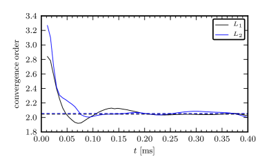
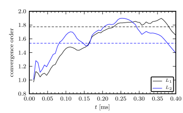
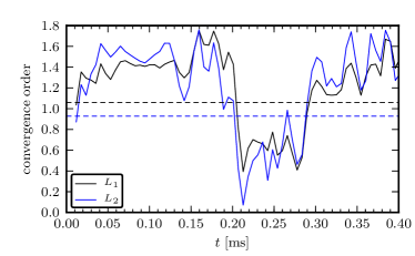
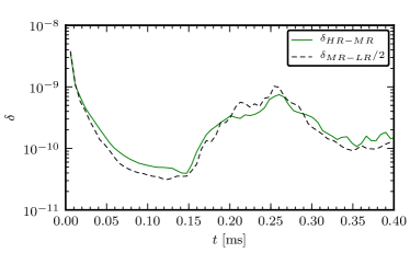
We evolved the system with three different grid spacings , , and , where , and . For the spherical grid, on which the optical depth is computed, we use a fixed radial resolution of . The reason is that we want to measure the convergence order of the evolution scheme, not the one of the interpolation to and from the spherical grid. We assume that for the chosen resolution, the interpolation error is not the dominant one.
Assuming a convergence behavior for the error of any evolved quantity , we estimate the convergence order of our simulations from the expression
| (108) |
which becomes exact in the limit of infinite resolution. We consider different norms to use in the formula above. In detail, we compute the discrete - and -norms over all grid points of the finest level that are present for each grid spacing and located on the equatorial plane. By doing this at each time step (common to all resolutions), we obtain a time dependent convergence order. Experience tells us that such measures can be quite noisy at practical resolutions. Therefore, we also use a global norm in Eq. (108) defined by the time average of the spatial norms. From this, we obtain a convergence order for the whole simulation. We evaluate those measures for three representative variables, namely the lapse , the energy density , and the emissivity of the electron-antineutrino.
In Fig. 16, the top left panel shows the time evolution of the convergence order for the lapse function. As described in Sec. II.1, we use a fourth order finite difference scheme for the evolution of the spacetime. However, after few crossing times of the finest grid the error of the lapse becomes dominated by the error of the fluid in the bulk of the star. The reconstruction scheme used for the hydrodynamical variables is expected to be at most second order and it is not surprising that this is also the order found for the evolution of the spacetime quantities.
As can be seen in the top right panel, the evolution of the energy density converges on average with order 1.7 with respect to the -norm, and with order 1.5 for the -norm. Those are typical values that can be expected from the PPM reconstruction procedure. Initially, however the error is dominated by the treatment of the surface and only during the rapid infall of the matter we recover the expected order of convergence.
The lower panels show the error of the effective electron-neutrino luminosity. In the right panel we show the residuals between high and medium resolution, as well as medium and low resolution, the latter rescaled assuming a convergence order of 1. The left panel depicts the convergence order. We find that the neutrino sources are at most first order accurate, as expected from the linear spatial interpolation from the spherical to the Cartesian grid and because of the first order accurate calculation of the optical depth. After the initial , which are dominated by the rapid cooling of the surface region, the model develops a convective layer in the outer envelope as described in Sec. VII. This causes the temporary dip seen in the convergence order, since it is notoriously difficult to resolve convective movements numerically. As we could see from this analysis, the formal convergence order of our evolution is one, limited by the lowest order part the scheme which is the computation of the neutrino sources. However in most astrophysical scenarios described with the NLS, the neutrinos are only of secondary importance in the dynamics of the system and for this reason a higher convergence order can be expected for the fluid quantities.
Appendix C Transformation from conserved to primitive variables
One of the most error prone parts of relativistic-hydrodynamic codes is the conversion from the evolved conserved variables to the primitive variables, which cannot be expressed in closed analytic form and requires some sort of root finding procedure. Moreover, there are corner cases for which numerical errors in the evolution lead to conserved variables which violate physical bounds, in some cases such that no solution exists at all. Those corner cases appear frequently at fluid-vacuum boundaries, e.g., NS surfaces, or close to the center of black holes. In both cases it is however possible to apply corrections such that the bulk behavior of the system is not influenced too strongly by the few affected grid points. Using tabulated EOSs further complicates the problem because the validity range of such EOS is limited, and because their derivatives tend to be noisy. It is crucial to have a scheme that takes all those corner cases into account, and that is able to apply corrections in a clearly defined way if necessary. In the following, we discuss the corner cases and present a scheme that is able to recognize them and take actions based on an error policy that can be chosen based on the problem at hand. Further, we describe the error policy used for the simulations in this article.
For convenience, we introduce the following definitions
| (109) | ||||||||
| (110) | ||||||||
It is easy to show the following relations
| (111) |
and further
| (112) | ||||
| (113) |
Equation of state requirements
For the recovery procedure, the only function needed to describe the EOS is . Derivatives are not required. It is crucial for our scheme that the EOS satisfies a few reasonable constraints. First, the matter should satisfy the dominant energy condition, i.e., the pressure should be smaller than the total energy density. We also exclude negative pressure. Second, the sound speed computed under the assumption of constant has to be real valued and smaller than the speed of light, i.e., the EOS should respect causality. We thus strictly require that
| (114) | ||||
| (115) |
where is the sound speed at constant composition.
Not all values of are physically meaningful. Moreover, the range in which the EOS is known or valid might be limited. This information is crucial in order to deal with corner cases correctly. We therefore define a validity region for each EOS by
| (116) | ||||
| (117) | ||||
| (118) |
Note the validity range for the internal energy depends on density and electron fraction. Usually, the lower bound is the zero-temperature limit. Note also we require positive internal energy. This is not a restriction on the EOS, but a restriction on the formal baryon mass constant used to define rest-mass density in terms of the baryon number density.
Bounds for the conserved variables
The conserved variables are subject to some physical and technical constraints, which we will derive in the following.
Since the baryon number density is always positive, we obviously require . For the benefit of the evolution scheme, we also require that , which implies . This is not essential to the recovery scheme, however. Requiring the total energy density to be nonnegative implies . Moreover, we require , which leads to
| (119) |
The conserved tracer for the electron fraction is trivially limited by , since .
Next, we compute bounds on the total momentum density, expressed in terms of the variable . We start from
| (120) |
Together with Eq. (114), we obtain the following order
| (121) |
The inequality is a direct consequence of the dominant energy condition. In terms of the evolved variables, it is equivalent to . If we decide to limit the velocity admitted during an evolution to a certain value , we obtain a necessary (but not sufficient) condition for
| (122) |
If any of those bounds is violated, it depends on the error handling policy whether the run is aborted or the values are adjusted such that the bounds are satisfied. If the policy allows it, we make the following adjustments. First, if , we set all variables to artificial atmosphere with , and , with . If we set while keeping and constant. If , we rescale the conserved momentum density such that . Finally, the electron fraction is limited to the allowed range.
Note that satisfying the above bounds for the conserved variables does not guarantee a valid solution yet. It however allows to safely compute values of the primitive variables using the method described in the following. The result will then be subject to further checks.
Solving for the primitive variables
We formulate the problem of computing the primitive variables as a root finding problem for some scalar function . There are many choices, not all of which are well behaved and efficient. Since we already have a bracketing of the velocity, it seems natural to choose the velocity as the independent variable. However, it has proven advantageous to use the equivalent quantity to eliminate all problems for strongly relativistic cases. For given conserved variables, we can use Eqs. (111)–(113) to express primitive variables as functions of , defining
| (123) | ||||
| (124) |
Note we replaced in Eq. (112) by an equivalent expression that is numerically more accurate for small velocities. The electron fraction, which can be computed directly from the evolved tracer variable, plays the role of a fixed parameter in the following and will be omitted to shorten notation.
The functions defined by Eqs. (123)–(124) are smooth and free of singularities for all values of . However, they can produce values for outside the validity range of the EOS. In order to avoid having to take this into account during the root finding procedure, we simply extend the EOS function to by the prescription
| (125) | ||||
| (126) | ||||
| (127) |
Next, we define
| (128) | ||||
| (129) |
Finally, we obtain the desired function from Eq. (111)
| (130) |
This function is well behaved for all values of . In the Newtonian limit, it is even linear. Due to Eq. (121) any root is confined to the interval given by
| (131) |
Note this bracketing is quite tight. In the Newtonian limit the upper bound becomes an equality, i.e., . We now show that always has a root in the above interval. First, we express as
| (132) |
A straightforward computation then yields
| (133) |
Since is continuous, we have shown the existence of a root. Once it is found, the velocity is computed from
| (134) |
The root can still correspond to an invalid solution, in the sense that lies outside the validity range of the EOS, or that . If the error policy allows it, we make the following adjustments. First, if , we set all variables to the artificial atmosphere values. Second, if the specific energy density is not in the EOS validity range Eq. (117), we replace , while keeping density and velocity constant. In terms of the conserved variables, this means keeping and constant while changing according to
| (135) |
Finally, if , we rescale the velocity such that , keeping constant. Since this slightly increases (due to the Lorentz factor), we also limit again to the range allowed at the adjusted density. In case of adjustments, pressure and conserved variables are also recomputed consistently.
In order to determine the root of numerically, we use the Illinois algorithm, a variant of the regula falsi method with superlinear convergence. This method is very robust since it keeps the root bracketed, never evaluates the function outside the initial interval, and most importantly does not require derivatives. Given the current status of tabulated EOSs, one cannot assume that the EOS is reasonable smooth or that the derivatives are meaningful everywhere. This discourages the use of root finding methods which require a derivative, e.g., Newton-Raphson.
We tested our method over a large parameter range. The number of required iterations to determine with an accuracy better than depends mainly on the Lorentz factor and only weakly on density and temperature. For the case of the LS-EOS, only calls to the EOS are required if , while calls are still sufficient for Lorentz factors up to .
Uniqueness of the solution
Now that we have shown that a solution exists, we need to prove that it is also unique. Since is continuous, we only have to show that at any root. For arbitrary , we find
| (136) | ||||
For a solution , we can rewrite this as
| (137) | ||||
If the solution is valid, . We then find that , where is the sound speed at constant electron fraction, and hence . With that we have proven that to each physically meaningful set of conserved variables, there exists exactly one set of primitives. In order to show that there is no additional invalid solution either, one can simply verify numerically that along the boundaries of the validity region of a given EOS.
Error handling policy
In the following, we present the error policy that determines under what conditions unphysical values of the evolved variables are corrected, as described previously, and when to abort the run. Most errors occur at stellar surfaces, where the densities are low and corrections therefore have a minor (but not negligible) impact on the global dynamics. We therefore consider some errors tolerable for low densities . Further, we are more lenient in a region near the center of black holes, which we define in terms of the lapse function , where the constant is chosen on a case by case basis such that it occurs only well inside the apparent horizon. One harmless error that occurs frequently when evolving zero-temperature initial data is that , simply because corresponds to the zero (or low) temperature limit and even small numerical errors can push below that boundary. In detail, we distinguish the following cases:
-
1.
. Never an error, adjust .
-
2.
. Adjust for low density or at BH center, else fatal error.
-
3.
. Never an error, set everything to atmosphere.
-
4.
. Always a fatal error.
-
5.
. Adjust velocity for low density or at BH center, else fatal error.
-
6.
out of range. Adjust electron fraction for low density or at BH center, else fatal error.
References
- Bauswein et al. (2012) A. Bauswein, H.-T. Janka, K. Hebeler, and A. Schwenk, Phys. Rev. D 86, 063001 (2012).
- Baiotti et al. (2005a) L. Baiotti, I. Hawke, P. J. Montero, F. Löffler, L. Rezzolla, N. Stergioulas, J. A. Font, and E. Seidel, Phys. Rev. D 71, 024035 (2005a).
- Abbott et al. (2009) B. P. Abbott et al. (LIGO Scientific Collaboration), Phys. Rev. D 80, 047101 (2009).
- Acernese et al. (2009) F. Acernese et al. (Virgo), Class. Quantum Grav. 26, 085009 (2009).
- Kuroda et al. (2010) K. Kuroda et al. (LCGT Collaboration), Classical and Quantum Gravity 27, 084004 (2010).
- Hinderer et al. (2010) T. Hinderer, B. D. Lackey, R. N. Lang, and J. S. Read, Phys. Rev. D 81, 123016 (2010).
- Eichler et al. (1989) D. Eichler, M. Livio, T. Piran, and D. N. Schramm, Nature 340, 126 (1989).
- Rezzolla et al. (2011) L. Rezzolla, B. Giacomazzo, L. Baiotti, J. Granot, C. Kouveliotou, and M. A. Aloy, Astrophys. J. 732, L6 (2011).
- Lattimer and Prakash (2001) J. M. Lattimer and M. Prakash, Astrophys. J. 550, 426 (2001).
- Haensel et al. (2007) P. Haensel, A. Y. Potekhin, and D. G. Yakovlev, Neutron Stars 1, 1st ed. (Springer-Verlag, New York, 2007).
- Lattimer (2012) J. M. Lattimer, Annu. Rev. Nucl. Part. Sci. 62, 485 (2012).
- Demorest et al. (2010) P. B. Demorest, T. Pennucci, S. M. Ransom, M. S. E. Roberts, and J. W. T. Hessels, Nature 467, 1081 (2010).
- Antoniadis et al. (2013) J. Antoniadis, P. C. C. Freire, N. Wex, T. M. Tauris, R. S. Lynch, M. H. van Kerkwijk, M. Kramer, C. Bassa, V. S. Dhillon, T. Driebe, J. W. T. Hessels, V. M. Kaspi, V. I. Kondratiev, N. Langer, T. R. Marsh, M. A. McLaughlin, T. T. Pennucci, S. M. Ransom, I. H. Stairs, J. van Leeuwen, J. P. W. Verbiest, and D. G. Whelan, Science 340, 448 (2013).
- Özel et al. (2010) F. Özel, G. Baym, and T. Güver, Phys. Rev. D 82, 101301 (2010).
- Steiner et al. (2010) A. W. Steiner, J. M. Lattimer, and E. F. Brown, Astrophys. J. 722, 33 (2010).
- Lattimer and Swesty (1991) J. M. Lattimer and F. D. Swesty, Nucl. Phys. A 535, 331 (1991).
- Shen et al. (1998a) H. Shen, H. Toki, K. Oyamatsu, and K. Sumiyoshi, Nucl. Phys. A 637, 435 (1998a).
- Shen et al. (1998b) H. Shen, H. Toki, K. Oyamatsu, and K. Sumiyoshi, Prog. Th. Phys. 100, 1013 (1998b).
- Shen et al. (2010) G. Shen, C. J. Horowitz, and S. Teige, Phys. Rev. C 82, 015806 (2010).
- Shen et al. (2011) G. Shen, C. J. Horowitz, and S. Teige, Phys. Rev. C 83, 035802 (2011).
- Hebeler et al. (2013) K. Hebeler, J. M. Lattimer, C. J. Pethick, and A. Schwenk, Astrophys. J. 773, 11 (2013).
- Faber and Rasio (2012) J. A. Faber and F. A. Rasio, Living Reviews in Relativity 15 (2012).
- Sekiguchi et al. (2011a) Y. Sekiguchi, K. Kiuchi, K. Kyutoku, and M. Shibata, Phys. Rev. Lett. 107, 051102 (2011a).
- Sekiguchi et al. (2011b) Y. Sekiguchi, K. Kiuchi, K. Kyutoku, and M. Shibata, Physical Review Letters 107, 211101 (2011b).
- Ruffert et al. (1996) M. Ruffert, H.-T. Janka, and G. Schäfer, Astron. Astrophys. 311, 532 (1996).
- Ruffert et al. (1997) M. Ruffert, H.-T. Janka, K. Takahashi, and G. Schaefer, Astron. Astrophys. 319, 122 (1997).
- Ruffert and Janka (2001) M. Ruffert and H.-T. Janka, Astron. Astrophys. 380, 544 (2001).
- Rosswog and Liebendörfer (2003) S. Rosswog and M. Liebendörfer, Mon. Not. R. Astron. Soc. 342, 673 (2003).
- Baiotti et al. (2003) L. Baiotti, I. Hawke, P. Montero, and L. Rezzolla, in Computational Astrophysics in Italy: Methods and Tools, Vol. 1, edited by R. Capuzzo-Dolcetta (MSAIt, Trieste, 2003) p. 210.
- Baiotti et al. (2005b) L. Baiotti, I. Hawke, L. Rezzolla, and E. Schnetter, Phys. Rev. Lett. 94, 131101 (2005b).
- Abdikamalov et al. (2012) E. Abdikamalov, A. Burrows, C. D. Ott, F. Löffler, E. O’Connor, J. C. Dolence, and E. Schnetter, Astrophys. J. 755, 111 (2012).
- Scheck et al. (2006) L. Scheck, K. Kifonidis, H.-T. Janka, and E. Müller, Astron. Astrophys. 457, 963 (2006).
- Mezzacappa and Bruenn (1993) A. Mezzacappa and S. W. Bruenn, Astrophys. J. 405, 637 (1993).
- Liebendörfer et al. (2009) M. Liebendörfer, S. C. Whitehouse, and T. Fischer, Astrophys. J. 698, 1174 (2009).
- Radice et al. (2013) D. Radice, E. Abdikamalov, L. Rezzolla, and C. D. Ott, J. Comput. Phys. 242, 648 (2013).
- Baiotti et al. (2008) L. Baiotti, B. Giacomazzo, and L. Rezzolla, Phys. Rev. D 78, 084033 (2008).
- Nakamura et al. (1987) T. Nakamura, K. Oohara, and Y. Kojima, Prog. Theor. Phys. Suppl. 90, 1 (1987).
- Shibata and Nakamura (1995) M. Shibata and T. Nakamura, Phys. Rev. D 52, 5428 (1995).
- Baumgarte and Shapiro (1998) T. W. Baumgarte and S. L. Shapiro, Phys. Rev. D 59, 024007 (1998).
- Bona et al. (1995) C. Bona, J. Massó, E. Seidel, and J. Stela, Phys. Rev. Lett. 75, 600 (1995).
- Alcubierre et al. (2003) M. Alcubierre, B. Brügmann, P. Diener, M. Koppitz, D. Pollney, E. Seidel, and R. Takahashi, Phys. Rev. D 67, 084023 (2003).
- Alic et al. (2010) D. Alic, L. Rezzolla, I. Hinder, and P. Mösta, Classical Quantum Gravity 27, 245023 (2010).
- Löffler et al. (2012) F. Löffler, J. Faber, E. Bentivegna, T. Bode, P. Diener, R. Haas, I. Hinder, B. C. Mundim, C. D. Ott, E. Schnetter, G. Allen, M. Campanelli, and P. Laguna, Class. Quantum Grav. 29, 115001 (2012).
- Timmes and Swesty (2000) F. X. Timmes and F. D. Swesty, Astrophysical Journal, Supplement 126, 501 (2000).
- Palenzuela et al. (2009) C. Palenzuela, L. Lehner, O. Reula, and L. Rezzolla, Mon. Not. R. Astron. Soc. 394, 1727 (2009).
- Martí et al. (1991) J. M. Martí, J. M. Ibáñez, and J. A. Miralles, Phys. Rev. D 43, 3794 (1991).
- Banyuls et al. (1997) F. Banyuls, J. A. Font, J. M. Ibáñez, J. M. Martí, and J. A. Miralles, Astrophys. J. 476, 221 (1997).
- Font (2008) J. A. Font, Living Rev. Relativ. 6, 4; http://www.livingreviews.org/lrr (2008).
- Janka et al. (1993) H.-T. Janka, T. Zwerger, and R. Mönchmeyer, Astron. Astrophys. 268, 360 (1993).
- Marek and Janka (2009) A. Marek and H.-T. Janka, Astrophysical Journal 694, 664 (2009).
- van Riper and Lattimer (1981) K. A. van Riper and J. M. Lattimer, Astrophys. J. 249, 270 (1981).
- Ruffert and Janka (1999) M. Ruffert and H.-T. Janka, Astron. Astrophys. 344, 573 (1999).
- Rosswog and Davies (2003) S. Rosswog and M. Davies, Mon.Not.Roy.Astron.Soc. 345, 1077 (2003).
- Rosswog et al. (2003) S. Rosswog, E. Ramirez-Ruiz, and M. B. Davies, Mon. Not. R. Astron. Soc. 345, 1077 (2003).
- Sekiguchi (2010) Y. Sekiguchi, Progress of Theoretical Physics 124, 331 (2010).
- O’Connor and Ott (2010) E. O’Connor and C. D. Ott, Classical Quantum Gravity 27, 114103 (2010).
- Ott et al. (2012) C. D. Ott, E. Abdikamalov, E. O’Connor, C. Reisswig, R. Haas, P. Kalmus, S. Drasco, A. Burrows, and E. Schnetter, Phys. Rev. D 86, 024026 (2012).
- Ott et al. (2013) C. D. Ott, E. Abdikamalov, P. Mösta, R. Haas, S. Drasco, E. P. O’Connor, C. Reisswig, C. A. Meakin, and E. Schnetter, Astrophys. J. 768, 115 (2013).
- Peres et al. (2013) B. Peres, M. Oertel, and J. Novak, Phys. Rev. D 87, 043006 (2013).
- Deaton et al. (2013) M. B. Deaton, M. D. Duez, F. Foucart, E. O’Connor, C. D. Ott, L. E. Kidder, C. D. Muhlberger, M. A. Scheel, and B. Szilagyi, ArXiv e-prints (2013).
- Mihalas and Mihalas (1984) D. Mihalas and B. Mihalas, New York: Oxford University Press, 1984 (1984).
- Baumgarte et al. (1996) T. W. Baumgarte, S. L. Shapiro, and S. A. Teukolsky, Astrophys. J. 458, 680 (1996).
- Baiotti et al. (2007) L. Baiotti, I. Hawke, and L. Rezzolla, Classical Quantum Gravity 24, S187 (2007).
- Rezzolla et al. (2010) L. Rezzolla, L. Baiotti, B. Giacomazzo, D. Link, and J. A. Font, Classical Quantum Gravity 27, 114105 (2010).
- Freiburghaus et al. (1999) C. Freiburghaus, S. Rosswog, and F.-K. Thielemann, Astrophys. J. 525, L121 (1999).
- Shibata et al. (2005) M. Shibata, K. Taniguchi, and K. Uryū, Phys. Rev. D 71, 084021 (2005).
- Bauswein et al. (2010) A. Bauswein, H. Janka, and R. Oechslin, Phys. Rev. D 82, 084043 (2010).
- Tondeur et al. (1984) F. Tondeur, M. Brack, M. Farine, and J. M. Pearson, Nuclear Physics A 420, 297 (1984).
- Swesty (1996) F. Swesty, Journal of Computational Physics 127, 118 (1996).
- Steffen (1990) M. Steffen, Astron. Astrophys. 239, 443 (1990).
- Colella and Woodward (1984) P. Colella and P. R. Woodward, J. Comput. Phys. 54, 174 (1984).
- Harten et al. (1983) A. Harten, P. D. Lax, and B. van Leer, SIAM Rev. 25, 35 (1983).
- Baiotti et al. (2009) L. Baiotti, B. Giacomazzo, and L. Rezzolla, Class. Quantum Grav. 26, 114005 (2009).
- Schnetter et al. (2004) E. Schnetter, S. H. Hawley, and I. Hawke, Class. Quantum Grav. 21, 1465 (2004).
- Thornburg (2004) J. Thornburg, Classical Quantum Gravity 21, 743 (2004).
- Baiotti and Rezzolla (2006) L. Baiotti and L. Rezzolla, Phys. Rev. Lett. 97, 141101 (2006).
- Kreiss and Oliger (1973) H. O. Kreiss and J. Oliger, Methods for the approximate solution of time dependent problems (GARP publication series No. 10, Geneva, 1973).
- Misner et al. (1973) C. W. Misner, K. S. Thorne, and J. A. Wheeler, Gravitation, Misner73 (W. H. Freeman, San Francisco, 1973).
- Shibata (1999) M. Shibata, Phys. Rev. D 60, 104052 (1999).
- Font et al. (2002) J. A. Font, T. Goodale, S. Iyer, M. Miller, L. Rezzolla, E. Seidel, N. Stergioulas, W. M. Suen, and M. Tobias, Phys. Rev. D 65, 084024 (2002).
- Duez et al. (2003) M. D. Duez, P. Marronetti, S. L. Shapiro, and T. W. Baumgarte, Phys. Rev. D 67, 024004 (2003).
- Giacomazzo and Rezzolla (2007) B. Giacomazzo and L. Rezzolla, Classical Quantum Gravity 24, S235 (2007).
- Cerdá-Durán et al. (2007) P. Cerdá-Durán, J. A. Font, and H. Dimmelmeier, Astron. Astrophys. 474, 169 (2007).
- Kastaun (2006) W. Kastaun, Phys. Rev. D 74, 124024 (2006).
- Dimmelmeier et al. (2006) H. Dimmelmeier, N. Stergioulas, and J. A. Font, Mon. Not. R. Astron. Soc. 368, 1609 (2006).
- Landau and Lifshitz (1976) L. D. Landau and E. M. Lifshitz, Mechanics, Volume 1 (Pergamon Press, Oxford, 1976).
- Zanotti et al. (2005) O. Zanotti, J. A. Font, L. Rezzolla, and P. J. Montero, Mon. Not. R. Astron. Soc. 356, 1371 (2005).
- Liebling et al. (2010) S. L. Liebling, L. Lehner, D. Neilsen, and C. Palenzuela, Phys. Rev. D 81, 124023 (2010).
- Radice et al. (2010) D. Radice, L. Rezzolla, and T. Kellerman, Classical Quantum Gravity 27, 235015 (2010).
- Radice and Rezzolla (2011) D. Radice and L. Rezzolla, Phys. Rev. D 84, 024010 (2011).
- Kastaun (2011) W. Kastaun, Phys. Rev. D 84, 124036 (2011).
- Cordero-Carrión et al. (2009) I. Cordero-Carrión, P. Cerdá-Durán, H. Dimmelmeier, J. L. Jaramillo, J. Novak, and E. Gourgoulhon, Phys. Rev. D 79, 024017 (2009).
- Hashimoto et al. (1994) M.-A. Hashimoto, K. Oyamatsu, and Y. Eriguchi, Astrophysical Journal 436, 257 (1994).
- Kaplan et al. (2013) J. D. Kaplan, C. D. Ott, E. P. O’Connor, K. Kiuchi, L. Roberts, and M. Duez, arXiv:1306.4034 (2013).
- Ibanez Cabanell (1981) J. M. Ibanez Cabanell, Mon. Not. R. Astron. Soc. 197, 845 (1981).
- Harrison et al. (1965) B. K. Harrison, K. S. Thorne, M. Wakano, and J. A. Wheeler, Gravitation Theory and Gravitational Collapse, Chicago: University of Chicago Press, 1965 (1965).
- Ipser (1970) J. R. Ipser, Astrophysics and Space Science 7, 361 (1970).
- Friedman et al. (1988) J. L. Friedman, J. R. Ipser, and R. D. Sorkin, Astrophys. J. 325, 722 (1988).
- Gondek et al. (1997) D. Gondek, P. Haensel, and J. L. Zdunik, Astron. Astrophys. 325, 217 (1997).
- Goussard et al. (1998) J. Goussard, P. Haensel, and J. L. Zdunik, Astron. Astrophys. 330, 1005 (1998).
- Takami et al. (2011) K. Takami, L. Rezzolla, and S. Yoshida, Mon. Not. R. Astron. Soc. 416, L1 (2011).
- Abdikamalov et al. (2009) E. B. Abdikamalov, H. Dimmelmeier, L. Rezzolla, and J. C. Miller, Mon. Not. R. Astron. Soc. 392, 52 (2009).
- Gourgoulhon and Haensel (1993) E. Gourgoulhon and P. Haensel, Astron. Astrophys. 271, 187 (1993).
- Chanmugam (1977) G. Chanmugam, Astrophysical Journal 217, 799 (1977).
- Gourgoulhon et al. (1995) E. Gourgoulhon, P. Haensel, and D. Gondek, Astron. Astrophys. 294, 747 (1995).
- Ledoux (1947) P. Ledoux, Astrophys. J. 105, 305 (1947).
- Epstein (1979) R. I. Epstein, Mon. Not. R. Astron. Soc. 188, 305 (1979).
- Keil et al. (1996) W. Keil, H.-T. Janka, and E. Mueller, Astrophysical Journal Letters 473, L111 (1996).
- Paschalidis et al. (2012) V. Paschalidis, Z. B. Etienne, and S. L. Shapiro, Phys. Rev. D 86, 064032 (2012).
- Wilson and Mathews (2003) J. R. Wilson and G. J. Mathews, Relativistic numerical hydrodynamics (Cambridge University Press, Cambridge, UK, 2003).
- Bruenn (1985) S. W. Bruenn, Astrophys. J. Suppl. 58, 771 (1985).
- Takahashi et al. (1978) K. Takahashi, M. F. El Eid, and W. Hillebrandt, Astron. Astrophys. 67, 185 (1978).
- Itoh et al. (1996) N. Itoh, A. Nishikawa, and Y. Kohyama, Astrophysical Journal 470, 1015 (1996).
- Yakovlev et al. (2001) D. G. Yakovlev, A. D. Kaminker, O. Y. Gnedin, and P. Haensel, Physics Reports 354, 1 (2001).
- Cooperstein et al. (1986) J. Cooperstein, L. J. van den Horn, and E. A. Baron, Astrophys. J. 309, 653 (1986).
- Cooperstein et al. (1987) J. Cooperstein, L. J. van den Horn, and E. Baron, Astrophys. J. Lett. 321, L129 (1987).
- Schinder et al. (1987) P. J. Schinder, D. N. Schramm, P. J. Wiita, S. H. Margolis, and D. L. Tubbs, Astrophys. J. 313, 531 (1987).
- Kantor and Gusakov (2007) E. M. Kantor and M. E. Gusakov, Mon. Not. R. Astron. Soc. 381, 1702 (2007).
- Haft et al. (1994) M. Haft, G. Raffelt, and A. Weiss, Astrophysical Journal 425, 222 (1994).
- Tubbs and Schramm (1975) D. L. Tubbs and D. N. Schramm, Astrophysical Journal 201, 467 (1975).