Testing gravitational-wave searches with numerical relativity waveforms: Results from the first Numerical INJection Analysis (NINJA) project
Abstract
The Numerical INJection Analysis (NINJA) project is a collaborative effort between members of the numerical relativity and gravitational-wave data analysis communities. The purpose of NINJA is to study the sensitivity of existing gravitational-wave search algorithms using numerically generated waveforms and to foster closer collaboration between the numerical relativity and data analysis communities. We describe the results of the first NINJA analysis which focused on gravitational waveforms from binary black hole coalescence. Ten numerical relativity groups contributed numerical data which were used to generate a set of gravitational-wave signals. These signals were injected into a simulated data set, designed to mimic the response of the Initial LIGO and Virgo gravitational-wave detectors. Nine groups analysed this data using search and parameter-estimation pipelines. Matched filter algorithms, un-modelled-burst searches and Bayesian parameter-estimation and model-selection algorithms were applied to the data. We report the efficiency of these search methods in detecting the numerical waveforms and measuring their parameters. We describe preliminary comparisons between the different search methods and suggest improvements for future NINJA analyses.
1 Introduction
Binary systems of compact objects, i.e., black holes and neutron stars, are among the most important objects for testing general relativity and studying its astrophysical implications [1]. The general solution of the binary problem in Newtonian gravity is given by the Keplerian orbits. In general relativity, the Keplerian orbits for a bound system decay due to the emission of gravitational radiation, leading eventually to the merger of the two compact objects and to a single final remnant [2, 3, 4]. The decay of the orbits is due to the emission of gravitational waves and these waves carry important information about the dynamics of the binary system. In particular, the waves produced during the merger phase contain important non-perturbative general relativistic effects potentially observable by gravitational-wave detectors. Gravitational waves could be detectable by the current generation of gravitational wave detectors such as LIGO and Virgo [5, 6], and detection is very likely with future generations of these detectors.
Two important advances have occurred in recent years that have brought us closer to the goal of observing and interpreting gravitational waves from coalescing compact objects. The first is the successful construction and operation of a world-wide network of large interferometric gravitational-wave detectors; these include the three LIGO detectors in the United States, Virgo in Italy, TAMA in Japan [7] and the GEO600 detector in Germany [8]. The TAMA detector was the first interferometric detector to achieve its design goals, and it collected science data between 1999 and 2003 [7]. The LIGO detectors started observations in 2002 [9]. From 2005 to 2007 these detectors operated at design sensitivity collecting more than a year of coincident data from the three LIGO detectors; these observations are referred to as the “fifth science run” (S5) [10]. The Virgo detector is also close to achieving its design goals and collected six months of data coincident with the last six months of the LIGO S5 run (referred to as VSR1) [11]. The GEO600 detector has been operating since in coincidence with the LIGO instruments [8]. The two 4km LIGO detectors are currently being upgraded to improve their sensitivity by a factor of 2–3 (Enhanced LIGO [205]) and will resume observations in 2009. Upgrades to the Virgo detectors to yield comparable sensitivity to Enhanced LIGO are proceeding on a similar schedule. During this time, the GEO600 and the LIGO Hanford 2km detector continue to make best-effort observations (called “astro-watch”) to capture any possible strong events, such as a galactic supernova. Following the Enhanced LIGO and Virgo observations, the Advanced LIGO [206] and Virgo [207] upgrades will improve detector sensitivities by a factor of above the Initial LIGO detectors; these upgrades are expected to be complete by 2014. There are also plans to build a second-generation cryogenic detector in Japan known as LCGT [12]. Searching data from these detectors for weak gravitational wave signals over a vast parameter space is a challenging task. The gravitational-wave community has invested significant resources in this effort. A number of searches on S5/VSR1 data for un-modelled bursts and binary coalescence are in progress and many results, including those from previous science runs, have already been reported [13, 14, 15, 16, 17, 18, 19, 20, 21, 22, 23].
The second important advance has been the impressive success of numerical relativity in simulating the merger phase of binary black hole (BBH) coalescence. The first breakthroughs occurred in 2005 with simulations by Pretorius [24], closely followed by the independent Goddard and Brownsville (now at RIT) results [25, 26]. Since then, a number of numerical relativity groups around the world have successfully evolved various configurations starting from the inspiral phase all the way through the merger to the final remnant black hole (for recent overviews on the field see e.g. [27, 28, 29]). This has led to important new physical insights in BBH mergers. These include the prediction of large recoil velocities produced by asymmetric emission of gravitational radiation during the merger process [30, 31, 32, 33, 34, 35, 36, 37, 38, 39, 40, 41, 42, 43, 44, 45, 46, 47, 48] and the prediction of the parameters of the remnant Kerr hole for a wide class of initial states [49, 32, 50, 51, 52, 53, 54, 55, 54, 56, 57, 58, 59, 60, 61]. Since the inspiral, merger and coalescence of black holes are also among the most important targets of gravitational-wave detectors, we expect that the detailed information provided by numerical simulations can be used to increase the reach and to quantify the efficacy of data analysis pipelines. Indeed the driving motivation of research on numerical simulations of black-hole binaries over the last few decades has been their use in gravitational-wave observations.
Thus far, most searches for gravitational waves from BBH mergers have relied on post-Newtonian results, which are valid when the black holes are sufficiently far apart. Within its range of validity, post-Newtonian theory provides a convenient analytic description of the expected signals produced by binary systems. The numerical relativity results, on the other hand, have not yet been synthesised into an analytic model for the merger phase covering a broad range of parameters, i.e., a wide range of mass ratios, spins and if necessary, eccentricity; there has however been significant progress for the non-spinning case [62, 51, 63, 64, 65, 66, 67, 68, 69, 70, 71, 72]. Similarly, despite significant progress, there is not yet a complete detailed description over the full parameter space of how post-Newtonian and numerical simulations are to be matched with each other. On the data analysis side, many pipelines, especially ones that rely on a detailed model for the signal waveform, have made a number of choices based on post-Newtonian results, and it is important to verify that these choices are sufficiently robust. More generally, it is necessary to quantify the performance of these data analysis pipelines for both detection and parameter estimation. This is critical for setting astrophysical upper limits in case no detection has been made, for following up interesting detection candidates, and of course for interpreting direct detections. Work on this to date has primarily used post-Newtonian waveforms. Numerical relativity now provides an important avenue for extending this to the merger phase.
There are significant challenges to be overcome before numerical relativity results can be fully exploited in data-analysis pipelines. The Numerical INJection Analysis (NINJA) project was started in the spring of 2008 with the aim of addressing these challenges and fostering close collaboration between numerical relativists and data analysts. Participation in NINJA is open to all scientists interested in numerical simulations and gravitational-wave data analysis. NINJA is the first project of its kind that attempts to form a close working collaboration between the numerical relativity and data analysis communities. Several decisions were made that restrict the scope of the results reported here: we consider only BBH simulations and have not used results from supernova simulations or simulations containing neutron stars; the waveform data comes purely from numerical simulations and we do not attempt to extend numerical data using post-Newtonian waveforms; the NINJA data set is constructed using Gaussian noise to model the response of the Initial LIGO and Virgo detectors – no attempt has been made to include non-Gaussian noise transients found in real detector data. The comparisons and conclusions reported here are thus necessarily limited, and in many cases are only the first steps towards fully understanding the sensitivity of data-analysis pipelines to black hole signals. Further studies are needed regarding the accuracy and comparison of numerical waveforms, and of how systematic errors in these waveforms can affect parameter estimation. Some analyses of numerical waveforms with regard to gravitational-wave detection have already been performed [73, 74, 64, 72], accuracy standards have been developed for use of numerical waveforms in data analysis [209] and a detailed comparison of some of the waveforms used in the NINJA project was performed in the related Samurai project [75]. We expect that subsequent NINJA analyses will build on these results to address these issues.
Despite the limited scope of the first NINJA project, we are able to draw the following broad conclusions from this work. Our first conclusion is that the current data analysis pipelines used to search LIGO, Virgo and GEO600 data for black hole coalescence are able to detect numerical waveforms injected into the NINJA data set at the expected sensitivities. Indeed, several of these pipelines are able to detect signals that lie outside the parameter space that they target. This is a non-trivial statement since most detectability estimates to date for these sources have relied on post-Newtonian waveforms, which are valid only when the black holes are sufficiently far apart. For many of these pipelines, this is the first time they have been tested against numerical waveforms. It should be noted, however, that the NINJA data set does not contain non-stationary noise transients so more work is needed to understand how detection performance is affected by the noise artifacts seen in real gravitational-wave detector data. Our second conclusion is that significant work is required to understand and improve the measurement of signal parameters. For instance, among the pipelines used in this first NINJA analysis only the Markov-chain Monte-Carlo algorithm attempted to estimate the spins of the individual black holes, and the estimation of the component masses by the detection pipelines is poor in most cases. Improvement in this area will be crucial for bridging the gap between gravitational wave observations and astrophysics. NINJA has proven to be extremely valuable at framing the questions that need to be answered.
This paper is organised as follows: In the next section we describe the contributed numerical waveforms and Section 3 describes the construction of the simulated gravitational-wave detector data used in the NINJA analyses. Descriptions of the search methods and results are given in Section 4. The results are grouped by search method into search pipelines using modelled waveforms (Section 4.1), search pipelines using un-modelled waveforms (Section 4.2) a comparison of inspiral-burst-ringdown results (Section 4.3), and Bayesian pipelines (Section 4.4). We conclude with a discussion of our results and future directions for NINJA in Section 5.
2 Numerical Waveforms
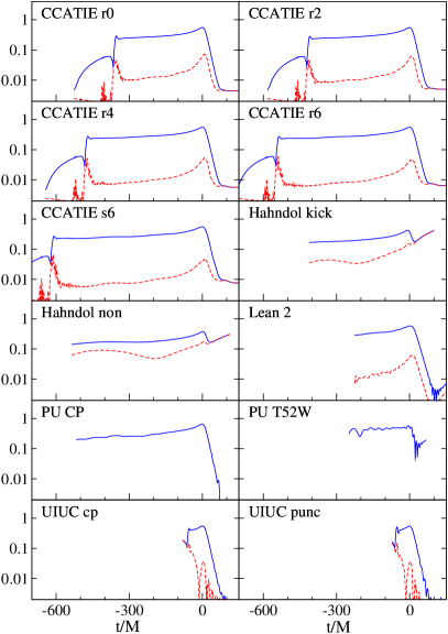
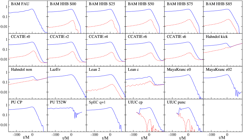
The NINJA project has studied BBH coalescence waveforms submitted by ten individuals and teams. Participation in NINJA was open to anyone and the only restrictions were that each contribution: (i) was a numerical solution of the full Einstein equations, (ii) consisted of only two waveforms, or up to five waveforms if they were part of a one-parameter family. No restrictions were placed on the accuracy of each waveform. All contributions followed the format specified in [76]. The waveforms are plotted in Figures 1 and 2. The contributed waveforms cover a variety of physical and numerical parameters. Most simulations model low-eccentricity inspiral, the mass ratio ranges from 1 to 4, and the simulations cover a range of spin configurations. The initial angular frequency of the mode ranges from to (where denotes the sum of the initial black-hole masses). This initial angular frequency marks where contributors consider the waveform sufficiently clean to represent the physical system (e.g. this will be chosen after initial unphysical radiation content, often referred to as “junk radiation” in numerical relativity, is radiated away). The length of the waveforms varies between a few 100M to over 4000M. The contributions naturally differ in accuracy, both regarding how well they capture the black-hole dynamics and in the extraction of the gravitational-wave signal. Table 1 lists a few key parameters that distinguish the waveforms, and introduces the following tags for the different contributions and codes: BAM HHB [77, 78, 79, 80, 81] and BAM FAU [77, 78, 60, 81] are contributions using the BAM code, CCATIE is the AEI/LSU code [82, 83, 34, 43, 52], Hahndol is the Goddard Space Flight Center’s code [84, 85], LazEv is the RIT code [86, 25, 46], Lean is Ulrich Sperhake’s code [87, 56, 88], MayaKranc is the Georgia Tech/Penn State code [74, 57], PU stands for the Princeton University code [89, 24, 62, 90], SpEC for the Cornell/Caltech collaboration code [91, 92, 66, 93], and UIUC stands for the University of Illinois at Urbana-Champaign team [94].
The codes listed above use different formulations of the Einstein equations, gauge conditions, mesh structures, initial data and wave extraction methods; we will attempt to give a unified presentation of common features first, and then list further details of the approaches separately for each contribution. Full details of each code are given in the references.
The numerical codes follow either of two approaches to solving the Einstein equations: (1) the generalised harmonic formulation, which was the basis of Pretorius’ initial breakthrough simulation of coalescing black holes [24], or (2) the moving-puncture approach, following [25, 26]. Both approaches result in canonical choices for the construction of initial data, the evolution system for the Einstein equations, and the treatment of the singularity inside the black-hole horizons.
| Code | Run | eccentricity | |||||
|---|---|---|---|---|---|---|---|
| Ref. | removal | ||||||
| BAM FAU | [60] | 1 | see caption | qc | 0.06 | T-PN [95, 55] | |
| [77, 78] | |||||||
| BAM HHB | S00 [79] | 1 | 0.045 | TR-PN [96] | |||
| [77, 78] | S25 [80] | 1 | 0.045 | T-PN [41] | |||
| S50 [80] | 1 | 0.052 | – ” – | ||||
| S75 [80] | 1 | 0.06 | – ” – | ||||
| S85 [80] | 1 | 0.06 | – ” – | ||||
| CCATIE | r0 [43] | 1 | , | qc | 0.079 | TR-PN [96] | |
| [82, 83, 34, 43] | r2 [43] | 1 | , | qc | 0.078 | – ” – | |
| r4 [43] | 1 | , | qc | 0.076 | – ” – | ||
| r6 [43] | 1 | , | qc | 0.075 | – ” – | ||
| s6 [52] | 1 | qc | 0.074 | – ” – | |||
| Hahndol | kick | 3 | , | qc | 0.078 | T-PN [97] | |
| [84, 85] | non | 4 | qc | 0.070 | – ” – | ||
| LazEv [86, 25] | MH [46] | 1 | qc | 0.07 | T-PN [97, 98] | ||
| Lean [87] | c | 4 | qc | 0.05 | T-PN [77] | ||
| 2 | 1 | qc | 0.11 | T-PN [97] | |||
| MayaKranc | e0 [57] | 1 | qc | 0.05 | TR-PN [96] | ||
| [74] | e02 [57] | 1 | 0.2 | 0.05 | n/a | ||
| PU [89, 24] | CP [62] | 1 | qc | 0.07 | T-ID [99] | ||
| T52W [90] | 1 | 0.07 | n/a | ||||
| SpEC [91] | q=1 [66, 93] | 1 | 0.033 | TR-it [92] | |||
| UIUC [94] | cp [94] | 1 | qc | 0.194 | T-ID [99] | ||
| punc [94] | 1 | qc | 0.203 | T-ID [100] |
| Code | Run | q | [s] | [Hz] | |
|---|---|---|---|---|---|
| BAM HHB | S00 | 1 | 1.03 | 15 | 48 |
| S25 | 1 | 1.15 | 15 | 48 | |
| S50 | 1 | 1.03 | 17 | 56 | |
| S75 | 1 | 0.81 | 19 | 65 | |
| S85 | 1 | 0.87 | 19 | 65 | |
| BAM FAU | 1 | 0.54 | 19 | 65 | |
| CCATIE | r0 | 1 | 0.34 | 26 | 85 |
| r2 | 1 | 0.37 | 25 | 84 | |
| r4 | 1 | 0.40 | 25 | 82 | |
| r6 | 1 | 0.45 | 24 | 81 | |
| s6 | 1 | 0.59 | 24 | 80 | |
| Hahndol | kick | 3 | 0.25 | 25 | 84 |
| non | 4 | 0.32 | 23 | 75 | |
| LazEv | MH | 1 | 0.43 | 23 | 75 |
| Lean | c | 4 | 0.92 | 16 | 54 |
| 2 | 1 | 0.20 | 36 | 118 | |
| MayaKranc | e0 | 1 | 1.23 | 16 | 54 |
| e02 | 1 | 0.74 | 16 | 54 | |
| PU | CP | 1 | 0.29 | 23 | 75 |
| T52W | 1 | 0.16 | 23 | 75 | |
| SpEC | q=1 | 1 | 1.96 | 11 | 36 |
| UIUC | cp | 1 | 0.10 | 63 | 209 |
| punc | 1 | 0.10 | 66 | 219 |
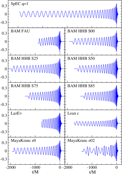
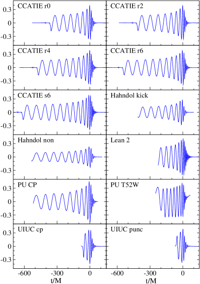
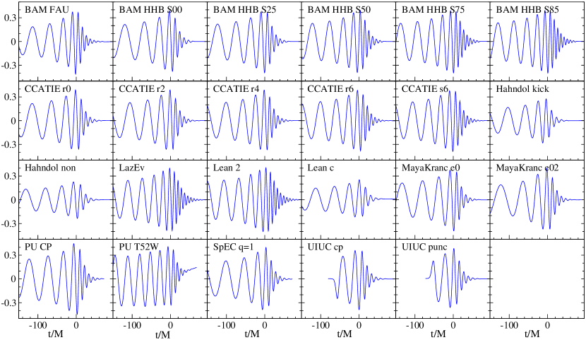
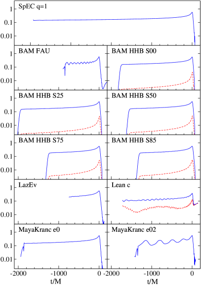
2.1 Summary of the simulation algorithms
2.1.1 Initial Data
Due to the presence of constraint equations, specifying initial data in numerical relativity is far from trivial, for a general overview see e.g. [101]. All of the results presented here make the simplifying assumption of conformal flatness for the spatial metric of the initial slice, which leads to some spurious gravitational radiation in the initial data. All contributions attempt to model non-eccentric inspiral, except for the two data sets PU–T52W and MayaKranc–e02. However, the degree of “quasi-circularity” varies, and in general one should bear in mind that the definition of eccentricity for fully general-relativistic orbits is not unique (see for example [56, 57]). The data set PU–T52W is notable for the fact that the BBH was constructed via scalar field collapse. Specifically, the initial data consists of two, compact, dense distributions of scalar field energy, separated by some distance and Lorentz boosted in opposite directions orthogonal to the line between them. Upon subsequent evolution, each scalar field pulse quickly collapses to form a black hole, with all remnant scalar field energy radiating away from the domain on the order of the light-crossing time of the orbit. This is the same time scale on which spurious gravitational radiation present in all current initial-data sets leaves the domain of the inspiral, and hence for practical purposes this can be considered a vacuum merger. All other runs start from vacuum initial data.
Most codes (BAM, CCATIE, Hahndol, LazEv, Lean, MayaKranc and the UIUC code) adopt the “moving puncture” approach, following [25, 26]. These codes use puncture initial data [102, 103, 104] to model black holes, resulting in initial data that contain a separate asymptotically flat end within each black hole. Constructing such initial data is mathematically well understood [103, 105]. The codes CCATIE, LazEv, Lean and MayaKranc all use the same pseudo-spectral solver for the Einstein constraint equations [106], and BAM uses a variant thereof [78]. UIUC-punc initial data is generated via the Lorene [107] multi-domain spectral libraries. The Hahndol code uses the second-order-accurate multi-grid solver amrmg [108], which is however tuned to give truncation errors typically much smaller than those produced by the evolution code.
The generalised harmonic codes use conformal thin sandwich initial data [109]. PU-CP and SpEC use quasi-equilibrium excision initial data where the interior of the black-hole horizons has been excised from the numerical grid. The presence of black holes with desired linear momenta and spins is enforced through the boundary conditions on the excision surfaces and the numerical outer boundary during the solution of the initial-value equations [110, 99, 111, 92]. This “excision technique” is based on the defining property of black holes — the horizons act as causal membranes and information cannot escape from the inside. The UIUC-cp simulation uses the same excised initial data, but fills the BH interior with “smooth junk”, as described in [94], before evolving with the moving puncture technique.
All codes take input parameters that ultimately determine the individual black-hole masses , spins , momenta and coordinate separation of the black holes (one should however be aware that in the strong field regime of general relativity various subtleties are associated with the definition of all of these quantities). In addition, the black-hole masses and dimensionless spins slowly change during the inspiral, which requires additional caution regarding the definition and accuracy of the values of mass, spin, etc. There are two common methods to estimate the instantaneous individual black-hole masses. One is to calculate the apparent-horizon mass, computed from the irreducible mass (given by the area of each hole’s horizon) and the spin according to Christodoulou’s [112] relation . The other, applicable only to puncture data, is to compute the Arnowitt-Deser-Misner (ADM) mass [113] at each puncture, which corresponds to spatial infinity in a space that contains only that black hole [104]. We generally use the total black-hole mass to scale dimensionful quantities, although sometimes the total conserved energy () is used for this purpose. Without loss of generality all codes chose the rest frame where and, thus, the net linear momentum vanishes initially.
Those simulations that attempt to model non-eccentric inspiral use initial parameters calculated by a number of different methods. Ideal initial parameters would produce tangential motion consistent with circular orbits, and radial motion consistent with slow inspiral. The various methods to choose initial parameters can be broadly characterised as those that attempt to provide only tangential motion (so that initially the black holes have no radial momenta), denoted by “T” in the last column of Tab. 1, and those that provide both tangential and radial motion (denoted by “TR”). The procedures to estimate these parameters are based on properties of the initial-data set (“ID”), post-Newtonian methods (“PN”), or an iterative procedure following the results of several trial simulations (“it”). In Tab. 1 we indicate which of these variants was used, and provide a reference to the specific algorithm; for the post-Newtonian methods in particular there are several variants. Note that the estimates of the resulting eccentricity range from (for the SpEC contribution) up to .
The two data sets from the UIUC contribution actually compare two alternative sets of non-spinning, equal-mass, quasi-circular initial data, with initial orbital frequency : (i) Puncture initial data with coordinate separation and initial linear momentum of each BH set according to [100], and (ii) Cook-Pfeiffer initial data with coordinate separation [114, 99] (measured from the centroids of the apparent horizons), filling the BH interior with data that smoothly connect to the exterior as described in [94]. Both data sets yield the same final spin , but differ at the level of a few percent in radiated energy and angular momentum.
For the eccentric MayaKranc simulation (data set e02), the conservative, third-post-Newtonian-order (3PN) expressions in Ref. [115] have been used to specify initial data. These expressions require the specification of the eccentricity and the mean motion , where is the radial (pericenter to pericenter) orbital period. There are three PN eccentricities, which are the same to 1PN order, and we choose , which appears in the PN Kepler equation, following Ref. [115]. The quantity has been chosen as () and . The binary separation, , was determined from equation (23) in Ref. [115], and the tangential linear momentum, =0.0498, of each black hole at apocenter was obtained from , where is the total angular momentum computed as a post-Newtonian expansion in and (equation (21) in Ref. [115]).
2.1.2 Evolution systems
There is a long history of casting the Einstein equations into systems of partial differential equations, and in particular into the form of a well-posed initial value problem. The process of writing the covariant Einstein equations in the form of three-dimensional tensor quantities that evolve in time is commonly referred to as a 3+1 split. The fundamental idea is to choose coordinates such that the spacetime metric can be written in the form
| (1) |
where is a positive-definite metric on the slices of constant time , and the scalar function and vector field are commonly used to encode the freedom of coordinate choice. They may in principle be freely specified, but in practice they are judiciously prescribed, usually through further evolution equations.
| Code | System | Technique | shift | ||||
|---|---|---|---|---|---|---|---|
| BAM HHB | BSSN | FD–6 | 000 | 2 | 56, 19 | ||
| BAM FAU | BSSN | FD–6 | 000 | 2 | |||
| CCATIE | BSSN | FD–4 | 000 | 1 | 20 | ||
| Hahndol | BSSN | FD– | 000 | 2 | 19, 13 | ||
| LazEv | BSSN | FD–4 | ttt | 6 | 1281 | 3.1 | |
| Lean | BSSN | FD– | 000 | 1.25,1 | , | , | 19, 13 |
| MayaKranc | BSSN | FD–4 | 000 | 2 | 16, 19 | ||
| PU | GH | FD–2 | n/a | n/a | |||
| SpEC | GH | Spectral | n/a | n/a | |||
| UIUC | BSSN | FD–4 | 000 | 0.25 | 25 |
The waveforms contributed to NINJA use versions of either of the two formulations for which successful multi-orbit evolutions of black-hole binaries have been published so far: the generalised harmonic and the BSSN/moving-puncture formulation of the Einstein equations. For overviews of writing the covariant Einstein equations as a time evolution problem, see e.g. [116, 117, 118].
The generalised harmonic formulation (see e.g. [118]) writes the evolution equations in manifestly hyperbolic form as a set of coupled wave equations for the space–time metric . The SpEC code uses this formulation in first order form [119], while the PU contribution is based on a second order version of the equations. Gauge conditions are enforced by specification of gauge-source functions , either as a specified function of time, or through evolution equations [24, 120, 66, 93].
All other codes use the first-order-in-time, second-order-in-space BSSN formulation of the Einstein evolution equations [121, 122, 123] in combination with hyperbolic evolution equations for the lapse and shift. The BSSN formulation consists of making a conformal decomposition of the spatial metric, , and all other variables, and the introduction of , which is treated as an independent variable. The moving-puncture treatment of the BSSN system involves evolving not the conformal factor but either (CCATIE), (BAM FAU, Hahndol [55, 124]), or (used by all other BSSN codes); it also consists of the gauge choices that we will summarise next.
All BSSN-based contributions evolve the lapse according to the 1+log slicing condition [125],
| (2) |
The shift vector field is evolved according to some variant of the -driver condition [83, 85]). During the evolution these gauge conditions change the geometry of the “puncture singularity” and soften the singularity as discussed in [126, 127, 128, 129].
The original -driver condition introduced in [83] is
| (3) |
The factor of is chosen such that at large distances the propagation speed of the hyperbolic equation (3) equals the coordinate speed of light [83], and the quantity is a parameter with the dimensions of the inverse of a mass and affects coordinate drifts: larger values of lead to a stronger initial growth of the apparent horizon, and thus to a magnification effect for the black holes [77]. Variants of this condition [25, 26, 130, 85, 131] consist of replacing some or all of the derivatives with . We will label these options with reference to each of the three time derivatives in (3): “ttt” denotes that is used for all three derivatives, “000” denotes usage of . The properties of the different choices are studied in [131, 85], and in [131] it is proven that the combination of the BSSN equations with the “1+log” slicing condition (2) and the “000” shift choice yields a well-posed initial-value problem.
Small differences in the evolutions also originate in the choice of initial lapse (all BSSN codes initialise the shift quantities and to zero). We first define a Brill-Lindquist-like conformal factor, , where is the distance to the th puncture, and and parametrise the masses of the black holes, although they are not in general equal to and . The RIT contributions choose , as does the Hahndol–non contribution, while the Hahndol–kick contribution uses an approximate derived from the late-time “1+log” Schwarzschild slicing [127]. BAM HHB, MayaKranc and the UIUC group use , and BAM FAU choose .
The generalised harmonic codes (PU and SpEC) employ black-hole excision, i.e., they excise from the computational grid a region around the singularities inside each black hole.
2.1.3 Radiation Extraction
All groups use one of two popular methods to estimate the gravitational-wave signal at a finite distance from the source: The SpEC and CCATIE contributions use the Zerilli-Moncrief/Sarbach-Tiglio perturbative formalism [132, 133, 134] (with SpEC following a version restricted to a Minkowski background in standard coordinates [135]), all other contributions use the Newman-Penrose curvature scalar . Both methods are implemented in the CCATIE code, and have been shown to give similar results [34, 43]). Summaries and details on the implementations within particular codes can be found, for instance in the references listed in Table 1. Since the gravitational-wave signal can only be defined unambiguously at null infinity, one typically considers several extraction radii and performs some form of convergence test, although for the present purpose most groups only report results for a single extraction radius. At finite radius both methods depend on the coordinate gauge, and the Newman-Penrose method additionally requires the choice of a tetrad, which is obtained by Gram-Schmidt orthonormalisation of a tetrad of coordinate vectors.
For this work, all waveforms have been contributed as spherical harmonic modes of spin-weight of the strain, according to the specification in [76]. Computation of the strain from the Zerilli-Moncrief odd- and even-parity multipoles of the metric perturbation requires one time integration [133, 43], in the Sarbach-Tiglio formalism the strain is algebraically related to the invariants at leading order in the inverse radius [136, 133], and computation of the strain from the Newman-Penrose curvature scalar requires two time integrations. Time integration requires the proper choice of integration constants, and may require further “cleaning procedures” to get rid of artifacts resulting from the finite extraction radii. For example, for the BAM HHB contribution unphysical linear drifts were removed by a variant of the method described in [70], where higher order than linear polynomials were used to remove unphysical drifts from higher modes to further improve the properties of the derived strain. In the RIT contribution, the strain was computed by taking the Fourier transform of , removing modes in a small region around , then dividing by and taking the inverse Fourier transform.
2.1.4 Numerical Methods and Computational Infrastructure
There are large overlaps regarding the numerical methods in the present waveform contributions. With the exception of the SpEC code, which uses a multi-domain pseudo-spectral method, all codes use finite-difference methods to discretise the equations. With the exception of the PU contribution, which uses a second-order-accurate implicit evolution scheme, all other codes use an explicit algorithm based on method of lines: Usually standard fourth-order-accurate Runge-Kutta time stepping, except for the SpEC code which uses a fifth order Cash–Karp time-stepper with adaptive step–size.
The moving-puncture/BSSN-based codes use standard centred finite differencing stencils; however the terms corresponding to the Lie-derivative with respect to the shift vector are off-centred (up-winded) by one grid-point. The CCATIE, MayaKranc, LazEv and UIUC codes use fourth-order-accurate stencils, the BAM code uses sixth-order stencils, the Hahndol code uses sixth-order stencils combined with fifth-order up-winded stencils [137], and the Lean code uses fourth-order for equal-mass and sixth-order for unequal-mass data sets. All of these codes add standard fifth-order Kreiss-Oliger dissipation [138, 139] to the right-hand-sides of the evolution equations. The finite-difference orders described here apply to the bulk of the computational domain. There are contributions at other orders in different parts of the codes, which we will describe below. However, the finite-difference order in the bulk plays the dominant role in defining the accuracy of the present simulations (and indeed the spatial finite-differencing order seems to dominate over the order of time integration when sufficiently small time steps are used), and for that reason we list in Tab. 3 the bulk spatial finite-difference order.
All codes except the SpEC code use variants of Berger-Oliger mesh-refinement. The PU and Hahndol codes employ full adaptive mesh refinement, while the other codes use a hierarchy of fixed refinement boxes which follow the motion of the black holes. Several of the codes are based on the Cactus computational toolkit [140, 141] and the Carpet mesh-refinement code [142, 143] (CCATIE, Lean, MayaKranc, LazEv, UIUC). The BAM HHB and BAM FAU contributions both use the BAM mesh refinement code. The Hahndol code uses the PARAMESH infrastructure [144] with a uniform time step; all other mesh refinement codes use a time step that depends on the grid spacing, and for these codes time interpolation at mesh-refinement boundaries introduces second-order errors.
For interpolation between meshes of different spacing, the groups that used fourth- or higher-order methods all use fifth-order-accurate (CCATIE, UIUC, LazEv, Lean, MayaKranc and Hahndol’s 4:1 “non” data) or sixth-order-accurate (BAM and Hahndol’s 3:1 “kick” data) polynomial interpolation in space between different refinement levels so that all spatial operations of the AMR method (i.e., restriction and prolongation) are sixth-order accurate and the second derivatives of interpolated values are at least fourth-order accurate.
A proper numerical treatment of gravitational waves in asymptotically flat spacetimes would include null infinity and not require boundary conditions at some finite distance from the source. Most codes circumvent this problem in essentially heuristic ways. The PU code uses spatial compactification combined with numerical dissipation, all BSSN codes use heuristic outgoing wave boundary conditions (which will in general violate constraint preservation and potentially well-posedness and will result in reflections of the outgoing radiation). The SpEC code, in contrast, uses constraint-preserving outer boundary conditions which are nearly transparent to outgoing gravitational radiation and gauge modes [145].
2.2 Accuracy
Estimates on accuracy are reported for the BAM HHB and SpEC contributions. For the BAM HHB simulations reasonably clean sixth-order convergence was observed, as reported in [79, 80]. In the waveform , extracted at , the uncertainty due to numerical errors and the use of finite extraction radii is estimated as 0.25 radians in the phase and less than 3% in the amplitude of the mode. Modes up to were calculated; the relative phase uncertainty is the same for all of them (the absolute phase uncertainty is proportional to ), but we estimate that the amplitude uncertainty increases to as much as for the highest modes. The SpEC contribution is the only one that extrapolates the gravitational wave signal to infinite extraction radius (using third-order polynomial extrapolation [66]). Various convergence tests indicate that the resulting extrapolated waveform is accurate to radians in phase and percent in amplitude [66].
3 Construction of the NINJA data set
The data provided by the numerical relativity groups follows the format outlined in [76], which is based on the mode decomposition of the gravitational radiation field at large distances from the source. If we specify a gravitational waveform in the Transverse-Traceless (TT) gauge, we only need the spatial components . We assume that we are sufficiently far away from the source so that the piece dominates:
| (4) |
where is the total mass of the system, is the distance from the source, and is a time-dependent TT tensor. In the TT gauge, has two independent polarisations denoted and and the complex function can be decomposed into modes using spin-weighted spherical harmonics of weight -2:
| (5) |
The expansion parameters are complex functions of the retarded time , however if we fix to be the radius of the sphere at which we extract waves then are functions of only. The angles and are respectively the polar and azimuthal angles in a suitable coordinate system centred on the source. This decomposition is directly applicable to non-precessing binaries. Otherwise, a comparison of the waveforms requires a careful treatment of mode-mixing effects due to rotations of the frame; see for instance [148]. The numerical data contributed to NINJA is given in the form of an ASCII data file for each mode , with accompanying meta-data describing the simulation [76]. Only modes that contribute appreciably to the final waveform are included, at the discretion of the contributing group. Each data file consists of three columns: time in units of the total mass, and the real and imaginary parts of the mode coefficients as a function of time. Note that the total mass scales both the time and the amplitude; thus the BBH waveforms for each simulation can be scaled to an arbitrary value of the mass. (This is not true in the case of simulations which include matter fields, but we do not consider such waveforms here.)
To model the signal seen by a gravitational-wave detector, we need to calculate the detector strain from the above mode decomposition. To do this, we must choose particular values of the total mass, orientation and distance from the detector. Given the , the total mass, the distance to the source, and the angles , we calculate using Equation. (5), and use the detector response functions (see, for example, Ref. [1]) to calculate the observed strain
| (6) |
Here are sky-angles in the detector frame, is the polarisation angle and the time is measured in seconds. In this analysis, we wish to simulate signals that might be observed by the Initial LIGO and Virgo detectors. There are three LIGO detectors: a 4 km detector and a 2 km detector at the LIGO Hanford Observatory (called H1 and H2, respectively) and a 4 km detector at the LIGO Livingston Observatory (called L1). The Virgo detector is a 3 km detector in Cascina, Italy (called V1). We used the same two-letter codes for the simulated NINJA detectors. Since the location and alignment of the three observatories differ, we must use the appropriate detector response and arrival time to compute the strain waveform seen at each observatory. This ensures that the waveforms are coherent between the detectors and simulate a true signal.
To model the detector noise, we generated independent Gaussian noise time series , sampled at Hz, for each detector. This sample rate was chosen to mimic that used in LSC-Virgo searches and assures a tolerable loss in signal-to-noise ratio due to the discrete time steps. Stationary white noise time series are generated and coloured by a number of time-domain filters designed to mimic the design response of each of the LIGO and Virgo detectors. Figure 3 shows the one-sided amplitude spectral density of each time detector’s time series, where is defined by
| (7) |
denotes the Fourier transform of and angle brackets denote averaging over many realisations of the noise.
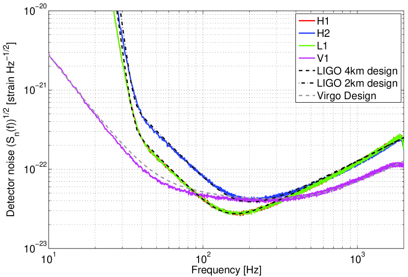
We see from Figure 3 that the noise power spectrum of the NINJA data set closely approximates the Initial LIGO design sensitivity in the frequency range of interest (- Hz). There is a slight discrepancy with the Virgo design curve at low frequencies (between approximately and Hz), which is an artefact of the Virgo noise generation procedure. Narrow-band features such as the violin and mirror modes were removed from the detector response used to compute the NINJA data, but were included in the calculation of the Virgo design curve [208]. The tails of these narrow-band features are responsible for the small discrepancy.
Having generated the simulated detector data, we then generated a population of simulated signals using the numerical relativity data. This population was constructed to cover a broad range of masses and signal amplitudes. We required that the starting frequency of the dominant mode of the signal was not more than Hz, an appropriate threshold given the sensitivity curve of the Initial LIGO and Virgo detectors. This sets a minimum mass at which each waveform can be injected, which is given in Table 2. The minimum possible injection mass is therefore . The maximum mass was chosen as . To get a good sample of long injected waveforms, we systematically chose a lower range of masses for the longer waveforms. No restrictions were placed on the other simulation parameters, i.e., the spins, mass-ratios and eccentricities. We ensured that waveforms from all the participating groups were equitably represented by generating approximately 12 signals from the waveforms supplied by each group. The time interval between adjacent injected signals was chosen to be a random number in the range s.
Given these constraints, we generated the parameters of the signal population. The logarithm of the distance to the binary was drawn from a uniform distribution ranging from Mpc to Mpc, and the source locations and orientations were drawn from an isotropic distribution of angles. We then computed waveforms corresponding to this population and at the appropriate sampling rate. We required that the optimal matched filter signal-to-noise ratio of any injection be greater than five in at least one of the four simulated detectors. Any waveform that did not satisfy this constraint was discarded from the population. Subject to this condition, the distances of injected signals varied from Mpc to Mpc (median at Mpc), the injected total mass range was (median at ), with individual component masses in the range .
Finally, the waveforms were added to the simulated detector noise to generate the NINJA data set . As described above, care was taken to ensure that signals were coherently injected in the data streams from the four detectors. The software for carrying out this procedure is freely available as part of the LSC Algorithm Library (LAL) [149].
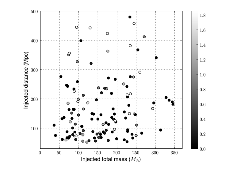
The data set used in this analysis consisted of a total of 126 signals injected in a total of 106 contiguous segments of noise each s long, thus spanning a duration of a little over hours. Figure 4 shows the mass, spin and distance of the waveforms contained in the NINJA data set.
4 Data Analysis Results
Analysis of the NINJA data was open to all and nine groups submitted contributions using a variety of analysis techniques. Participating groups were provided with the NINJA data set containing signals embedded in noise and the parameters of the injected signals. Analysts were not given access to the raw numerical-relativity waveforms or noiseless injection data.
Methods used to analyse the NINJA data include: matched-filter based searches, un-modelled waveform searches using excess-power techniques, and Bayesian model-selection and parameter-estimation techniques. Where possible, the performance of different searches is compared. The limited scope of the NINJA data set makes detailed comparisons difficult, however. A list of the data-analysis contributions is shown in Table 4.
| Group | Analysis | Section |
|---|---|---|
| AEI | Phenomenological Waveforms in CBC pipeline | 4.1.3 |
| Birmingham | Bayesian Model Selection | 4.4.2 |
| Cardiff | Post-Newtonian (PN) Templates in CBC pipeline | 4.1.1 |
| Cardiff, Maryland | EOBNR waveforms in CBC pipeline | 4.1.3 |
| Goddard | Hilbert Huang Transform | 4.2.2 |
| Northwestern | Markov Chain Monte Carlo | 4.4.1 |
| Syracuse | Extended PN Templates in CBC pipeline | 4.1.1 |
| UMass, Urbino | Q-pipeline analysis | 4.2.1 |
| UWM | PN templates in CBC pipeline, Neyman-Pearson criteria | 4.1.2 |
| UWM, UMass, Urbino | Ringdown analysis | 4.1.4 |
| UWM, UMass, Urbino | Inspiral, Merger, Ringdown combined search | 4.3 |
In sections 4.1 and 4.2 we describe results of analyses using modelled (matched-filter) and un-modelled waveforms, respectively. Comparisons between these analyses are given in Section 4.3 and Section 4.4 presents the results of Bayesian model-selection and parameter-estimation analyses.
4.1 Search pipelines using modelled waveforms
When the waveform of the target signal is known, matched filtering is the optimal search technique for recovering signals buried in stationary noise [150, 151]. This section describes the results of filtering the NINJA data with matched-filter based analysis pipelines. Results are given for waveforms that span only the inspiral signal, the ringdown alone, and the full inspiral, merger and ringdown. Although the morphologies of these waveforms differ, the underlying analysis techniques are similar in all cases. All the contributions in this section use a pipeline developed by the LSC and Virgo Collaboration to search for gravitational waves from binary neutron stars and black holes in a network of detectors [152, 17]. We first describe the features of this pipeline common to all the contributed matched-filter analyses before presenting the results of searching the NINJA data using different matched-filter templates.
The LSC-Virgo search pipeline performs a series of hierarchical operations in order to search for real signals buried in the detector noise: Given a desired search parameter space and waveform model, a “bank” of templates is created to cover the parameter space such that the fractional loss in signal-to-noise ratio (SNR) between any signal and the nearest template is less than a specified value (typically ). All the NINJA inspiral searches use a non-spinning template bank parametrised by the two component masses of the binary [153, 154, 155]. It has been found that inspiral searches for spinning binaries using waveforms which neglect the effect of spin are reasonably effective in most cases [152, 156]. Ringdown searches use a two parameter template bank parametrised by the frequency and quality factor of the signal constructed to cover the desired range of mass and spin [157]. Data from each of the detectors is separately match filtered against this bank of waveforms [158, 157] and a “trigger” is produced whenever the SNR exceeds the desired threshold. All the analyses used a threshold of . A test is then performed which discards triggers which do not have coincident parameters in two or more detectors (time and masses for inspiral searches, and time, mass and spin for ringdown searches) [159, 160]. These coincident triggers provide the gravitational-wave candidates for the ringdown analysis. The triggers are ranked by a detection statistic constructed from the SNRs of the individual triggers in a coincidence by . Coincident inspiral triggers are subject to a second stage of filtering in which “signal-based vetoes” are also calculated, which aim to separate true signals from noise fluctuations. These include the [161] and [162] tests. Signal-based vetoes could also be employed for ringdown searches, but at present they are not implemented in the pipeline. For each trigger, we construct an effective SNR , which combines the matched-filter SNR and the value of the signal based veto [161]. Explicitly, the effective SNR is defined as [152, 17]
| (8) |
where DOF signifies the number of degrees of freedom in the test. For signals of moderate SNR, which are a good match to the template waveform, the expected value of the is unity per degree of freedom and consequently the effective SNR is approximately equal to the SNR. Non-stationarities in the data typically have large values of and consequently the effective SNR is significantly lower than the SNR. A second test is then performed to discard coincidences in which signal-based vetoes reduce the number of triggers to less than two. These coincidences provide the candidate gravitational wave signals for the inspiral-based pipelines and they are ranked by the combined effective SNR . To evaluate the sensitivity of the analyses, we compare the list of gravitational-wave candidates generated by filtering the NINJA data to the parameters of the inject numerical relativity signals.
Six groups contributed matched-filter results to this analysis and the results can be roughly divided into three categories based on the waveform templates used: (i) searches based on the stationary-phase approximation to the inspiral signal, which are designed to capture various stages of the inspiral, merger and ringdown, (ii) searches which use waveforms designed to model the full inspiral-merger-ringdown signal, (iii) searches using ringdown-only waveforms obtained from black hole perturbation theory. Within these categories, different parameter choices were made in order to investigate the ability of the pipeline to detect the numerical relativity simulations. Each of these three approaches is described independently in the following sections. A comparison between these results is given in Section 4.3.
4.1.1 Stationary Phase Inspiral Templates
The workhorse template of the LSC-Virgo search pipeline is based on the stationary-phase approximation to the Fourier transform of the non-spinning post-Newtonian inspiral [163, 158]. This waveform (referred to as SPA or TaylorF2) has been used in the search for binary neutron stars [14, 15, 17, 13], sub-solar mass black holes [16, 17, 13] and stellar mass black holes [13]. The TaylorF2 waveform is parametrised by the binary’s component masses and (or equivalently the total mass and the symmetric mass ratio ) and an upper frequency cutoff . Amplitude evolution is modelled to leading order and phase evolution is modelled to a specified post-Newtonian order. In this section we investigate the performance of TaylorF2-based searches on the three simulated LIGO detectors. Results which include the simulated Virgo detector are described in the next section. Several analyses were performed which test the ability of TaylorF2 waveforms to detect numerical relativity signals. The analyses differed in the way the TaylorF2 waveforms or the template bank were constructed. The results of these searches are summarised in Table 5, each column giving the results from a different search with a summary of the chosen parameters. We first describe the parameters varied between these analyses and then present a more detailed discussion of the results.
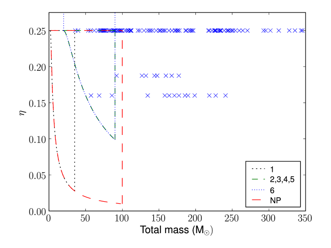
All TaylorF2 NINJA analyses used restricted templates (i.e. the amplitude is calculated to leading order), however the phase was calculated to various different post-Newtonian orders [164]. Phases were computed to either two [165, 166] or three point five post-Newtonian order [167, 168, 169] since these are, respectively, the order currently used in LSC-Virgo searches [13] and the highest order at which post-Newtonian corrections are known. After choosing a post-Newtonian order, one chooses a region of mass-parameter space to cover with the template bank. Figure 5 shows the boundaries of the template banks used in the analyses. One search used the range used by the LSC-Virgo “low-mass” search [13] () and all other searches used templates with total masses in the range . These boundaries were chosen since there were no signals in the NINJA data with mass smaller than and there is little, if any, inspiral power in the sensitive band of the NINJA data for signals with . The standard LSC-Virgo template bank generation code [154] restricts template generation to signals with , since it is not possible to invert and to obtain real-valued component masses for . All but one of the searches enforced this constraint, with the for the low-mass CBC search and for the other “physical-” searches. It is, however, possible to generate TaylorF2 waveforms with “unphysical” values of . In two separate studies using Goddard and Pretorius waveforms [64], and Caltech-Cornell waveforms [72] it was observed that match between numerical signals and TaylorF2 templates could be increased by relaxing the condition . One NINJA contribution uses a template bank with to explore this.
Finally, it is necessary to specify a cutoff frequency at which to terminate the TaylorF2 waveform. In the LSC-Virgo analyses, this is chosen to be the innermost stable circular orbit (ISCO) frequency for a test mass in a Schwarzschild spacetime
| (9) |
This cutoff was chosen as the point beyond which the TaylorF2 waveforms diverge significantly from the true evolution of the binary [164]. More recently, comparisons with numerical relativity waveforms have shown that extending the waveforms up to higher frequencies improves the sensitivity of TaylorF2 templates to higher mass signals [64, 72]. The NINJA TaylorF2 analyses use templates terminated at the ISCO frequency and two additional cut-off frequencies: the effective ringdown (ERD) frequency and a weighted ringdown ending (WRD) frequency. The ERD frequency was obtained by comparing post-Newtonian models to the Pretorius and Goddard waveforms [64]. The ERD almost coincides with the fundamental quasi-normal mode frequency of the black hole formed by the merger of an equal-mass non-spinning black-hole binary. The weighted ringdown ending (WRD) frequency lies between ISCO and ERD, and was obtained by comparing TaylorF2 waveforms to the Caltech-Cornell numerical signals [72].
| Analysis | ||||||
|---|---|---|---|---|---|---|
| Freq. Cutoff | ISCO | ISCO | ERD | ERD | WRD | WRD |
| PN Order | 2 PN | 2 PN | 2 PN | 3.5 PN | 3.5 PN | 3.5 PN |
| Total Mass | 2–35 | 20–90 | 20–90 | 20–90 | 20–90 | 20–90 |
| range | 0.03–0.25 | 0.10–0.25 | 0.10–0.25 | 0.10–0.25 | 0.10–0.25 | 0.10–1 |
|
Found Single
(H1, H2, L1) |
69, 66, 75 | 72, 43, 66 | 83, 51, 81 | 91, 56, 87 | 90, 55, 88 | 90, 56, 88 |
|
Found
Coincidence |
49 | 59 | 79 | 82 | 82 | 84 |
|
Found Second
Coincidence |
48 | 59 | 77 | 81 | 81 | 81 |
The results of these searches are reported in Table 5. The principal result is the number of injected signals detected by the search. For simplicity, we define a detected signal as one for which there is a candidate gravitational-wave signal observed within ms of the coalescence time of the injection, determined by the maximum gravitational-wave strain of the injected signal. We do not impose any additional threshold on the measured SNR or effective SNR of the candidate. For a single detector, this will lead to a small number of falsely identified injections, but for coincidence results the false alarm rate is so low that we can be confident that the triggers are associated with the injection. We now describe these results in the order that they appear in Table 5.
Search used second order post-Newtonian templates terminated at with a maximum mass of . Despite the fact that no NINJA injections had a mass within the range of this search, a significant number of signals were still recovered in coincidence both before and after signal consistency tests. Although the templates are not a particularly good match to the injected signals, they are still similar enough to produce triggers at the time of the injections. Search changed the boundary of the template bank to , but left all other parameters unchanged. The number of detected signals increases significantly as more signals now lie within the mass range searched.
Search extended the upper cutoff frequency of the waveforms to . The number of signals detected increased from 59 to 77, as expected since these waveforms can detect some of the power contained in the late inspiral or early merger part of the signal [64, 72]. Search extends the post-Newtonian order to 3.5 PN, slightly increasing the number of detected signals to 81. With the limited number of simulations performed in this first NINJA analysis, it is difficult to draw a strong conclusion, although there does seem to be evidence that the higher post-Newtonian order waveforms perform better, consistent with previous comparisons of post-Newtonian and numerical relativity waveforms [64, 170, 79, 71, 72]. Search uses an upper-frequency cutoff of for the templates. The number of injections found in coincidence for this search is the same as the search using order templates with a cutoff of , although there are slight differences in the number of found injections at the single detector level.
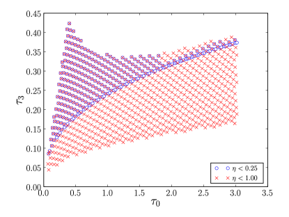
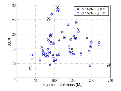
Search extends the template bank of search to unphysical values of the symmetric mass ratio. Extending the bank to increases the number of templates in the bank by a factor of . The original and modified template banks are shown in Figure 6. With the extended template bank the number of injections found in coincidence remains the same as search after signal-based vetoes are applied. However, many of the injections are recovered at a higher SNR, particular the low-mass signals, as shown in Figure 6. Some injections show a reduction in SNR; more work is needed to understand this effect.
Finally, we note that the majority of signals passed the signal-based veto with the thresholds used in the LSC-Virgo pipeline. The last two lines of Table 5 show the number of recovered signals before and after these signal-based vetoes are performed. The post-Newtonian templates and numerical relativity signals are similar enough that virtually all of the injected signals survive the signal based vetoes.
To illustrate the results of these analyses in more detail, Figure 7 shows which signals were detected and which were missed by the 3.5 order post-Newtonian TaylorF2 templates terminated at , as a function of injected total mass and effective distance of the binary (a measure of the amplitude of the signal in the detector), defined by [158]
| (10) |
where is the luminosity distance of the binary.
One signal, with total mass of and effective distance Mpc, was missed while others with similar parameters were found. This
signal was one of the Princeton waveforms (labelled PU-e0.5 in
Figure 1) for which the maximum amplitude occurs at the start
of the waveform rather than at coalescence111That the maximum
occurs at the start of the waveform is in part an “artifact” of the
double-time integration from the Newman-Penrose scalar to the
metric perturbation , and in part a coordinate artifact.
The two integration constants were chosen to remove a
constant and linear-in-time piece for , however, there is still
a non-negligible quadratic component; we suspect this is purely gauge,
though lacking a better understanding of this it was not removed from the
waveform., rendering our simple coincidence
test invalid. The injection finding algorithm compares the peak time to the
trigger time and, even though triggers are found at the time of the simulation,
there are no triggers within the ms window used to locate detected
signals.
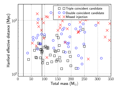
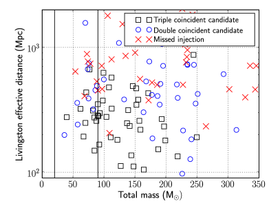
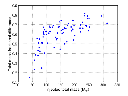
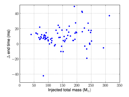
Figure 8 shows the accuracy with which the total mass and coalescence time of the binary are recovered when using the 3.5 post-Newtonian order Taylor F2 templates. The total mass fraction difference is computed as . For lower mass signals, the end time is recovered reasonably accurately, with accuracy decreasing for the high mass systems. The total mass recovery is poor for the majority of signals, with good parameter estimation for only a few of the lowest mass simulations.
4.1.2 Four-detector Inspiral Search
The inspiral analysis described in Section 4.1.1 considered data from the three simulated LIGO detectors. We now extend the analysis to include data from the simulated Virgo detector. In addition, we impose an alternative criterion, based on the Neyman-Pearson formalism [151], to determine those injections which were detected by the pipeline. In the previous section an injection was classified as found by the search if gravitational-wave candidate existed within 50 ms of the peak time of the numerical data. Here, we consider a signal to be found is there is an associated candidate whose significance exceeds a pre-determined threshold. Specifically, we require the candidate to have a significance greater than any candidate arising due to noise alone. This allows us to probe in more detail the effect of signal-based vetoes and the efficaciousness of the effective SNR statistic in analysis of the NINJA data.
Data from all four simulated NINJA detectors was analysed using the CBC pipeline as described in column of Table 5. In addition, a second analysis was performed with that the template bank extended to cover the region from , with all other parameters unchanged. The search can therefore be though of as the simplest extension of the standard LSC-Virgo “low mass” CBC search [13]. The boundary of the template bank used is shown in Figure 5.
In this analysis, we choose a detection statistic and claim that a gravitational-wave candidate is present if the value of this statistic exceeds a pre-determined threshold. All candidates are considered detections. The threshold is chosen so that the false alarm probability—the probability that a noise event will be mistaken for a real signal—is tolerable. The efficiency of this method depends on how close the chosen statistic is to the optimal detection statistic. It is well known that the matched filter SNR is the optimal statistic for known signals in a single detector if the noise is stationary [150, 151]. For a network of detectors containing stationary noise, the optimal statistic is the coherent signal-to-noise ratio [171]. At the time of this analysis, calculation of was not available in the CBC pipeline, so we instead compute a combined SNR from the detectors, , as a simple alternative. In the presence of non-Gaussian noise, the effective SNR, described in Section 4.1, has shown to be an effective detection statistic [17]. In this analysis, we also consider the combined effective SNR .
We investigate three choices of detection statistic: (i) the combined matched filter SNR of coincident candidates before signal-based vetoes are applied (), (ii) the combined matched filter signal-to-noise ratio after the signal-based veto has been applied applied to coincidences (), (iii) the combined effective SNR (). This statistic is only available after the second coincidence stage, since it is a function of matched filter SNR and the statistic for a candidate. To set a threshold for each statistic we choose the highest value of that statistic NINJA data containing only noise. To do this, we discard all triggers within s of an injected signal; the remaining triggers will be due to the simulated noise alone (we note that this approach is not possible in real data where the locations of the signals are unknown). This crude method of background estimation should provide us with consistent criteria for elimination of spurious detections. Therefore, we mark an injection as found only if it resulted in a trigger with statistic higher then any background trigger found in the data.
| Bank mass range | ||||
|---|---|---|---|---|
| Statistic | Statistic | Found | Statistic | Found |
| Threshold | Injections | Threshold | Injections | |
| 9.18 | 73 | 9.8 | 91 | |
| 9.18 | 69 | 9.8 | 93 | |
| 10.05 | 27 | 10.05 | 85 | |
Table 6 shows the threshold and the number of triggers found for each choice of statistic. It is interesting to compare the results for the low-mass search when we threshold on , rather than using a ms time window to determine detected signals. When using the time-window method, the number of injections found by the low-mass search is , but this increase to when using the the threshold method. Since all the injected signals lie outside the boundary of the low-mass bank, the coalescence time of the signals will be poorly estimated. This will result in triggers outside the ms window, which are nevertheless are loud enough to lie above the background.
Signal-based vetoes are applied at the second stage of the inspiral pipeline and are used to compute . By comparing the number of triggers found before and after signal-based vetoes are applied, we can evaluate their effect on the sensitivity of the search. Note that we observe the same threshold for both and . However, the number of detected signals in the low-mass search is reduced by 4 as the the veto has removed triggers where the templates are not a good match for the signals. More intriguing is a slight increase in the number of detected signals after the veto in the bank with the extended mass range (from to ). Additional investigations revealed that, despite having fewer triggers in each detector after the test has been applied, the total number of coincident triggers actually increases. This is due to the fact that the signal-based vetoes cause the time of the signal to be measured more accurately in the detectors; more triggers therefore survive the coincidence test. We do not observe this in the case of the low mass search.
Finally, we turn our attention to the effective SNR statistic, defined in equation (8). Since the NINJA detector noise is stationary and Gaussian, the expected value of the is one per degree of freedom. Therefore, we do not expect that the effective SNR will be useful in reducing the significance of loud background triggers. This is borne out by the fact that the statistic threshold actually increases slightly when using effective SNR. For the low mass search the number of signals found by thresholding on is significantly less than when using the combined SNR statistic. This is to be expected as the simulated signals do not match well with the templates. Although the low mass templates produce candidates, these will have large values of since signal and template do not match well. Thus, the effective SNR will be smaller than the original SNR and fewer signals will be recovered above the threshold. This effect is less significant for the second search with a larger mass range as the templates provide a better match to the simulated signals. Since effective SNR has been a powerful statistic in real detector data, this highlights the need for further NINJA studies using data containing non-stationary noise transients.
4.1.3 Inspiral-Merger-Ringdown Templates
The calculation of the full binary binary black hole coalescence waveform accessible to ground-based detectors requires numerical methods. At the moment, it is not possible to accurately model a coalescing binary over hundreds of orbits due to the computational cost of evolutions. Furthermore, it is not necessary to model the entire waveform, since post-Newtonian gives a valid description of the system when the black holes are sufficiently separated. During their final orbits before merger the black holes’ velocities increase and the post-Newtonian expansion becomes less reliable. At this stage the non-perturbative information contained in numerical simulations is required. A successful approach has been to combine analytical and numerical results to obtain full waveform templates. Two different families of such waveforms have been used to analyse the NINJA data: the effective one body (EOB) [172, 173, 174, 175] and phenomenological [63, 67] models.
By combining together results from post-Newtonian theory and perturbation theory, the EOB model [172, 173] predicts the full inspiral, merger and ringdown waveform. More recently, the non-spinning EOB model has been further improved by calibrating it to NR results, achieving high overlaps without the need to maximise the intrinsic mass parameters of the binary [62, 64, 65, 68, 69, 70, 71]. The LSC Algorithm Library (LAL) [149] contains two implementations of the effective one body template: one (called EOB) which only evolves the waveform to the light-ring frequency
| (11) |
and a second (called EOBNR) which implements the full EOB waveform described in [65]. This template which was constructed to match the NASA-Goddard binary black hole simulations with mass ratios : 1:1, 3:2, 2:1 and 4:1, however LAL waveforms do not yet implement higher harmonics of the signal. Both of these implementations were used to search for black hole binary signals in NINJA data.
Another approach for constructing the full waveform is to “stitch” together the results of post-Newtonian and numerical relativity calculations. The model presented in [63, 67, 176] consists of matching the post-Newtonian and numerical waveforms in an appropriate matching regime (where both are sufficiently accurate) to obtain a “hybrid” waveform. This hybrid is then fit by a phenomenological model in the frequency domain determined entirely by the physical parameters of the system. This procedure has been carried out for non-spinning black holes and a two-dimensional template family of waveforms that attempts to model the inspiral, merger and ringdown stages for non-spinning binary black holes has been obtained. Each waveform is parametrised by the physical parameters of the system, i.e., the masses and of the black holes.
Since the EOBNR and phenomenological models provide complete waveforms, the search was performed to higher masses ( and respectively) than for inspiral only searches. In principle, the search could be extended to even higher masses, but technical issues with the current waveform generation procedures prevent this. The minimum component mass was also increased, in an effort to reduce the size of the template bank by limiting the number of highly asymmetric signals. Finally, the template bank for all these searches was constructed using the standard second order post-Newtonian metric, and hexagonal placement algorithm [155]. At high masses, the parameter space metric for the full waveforms will differ significantly from the standard second-order post-Newtonian metric. However, the current template bank placement suffices for detection purposes, although probably not for good parameter estimation.
| Template | EOB | EOBNR | Phenom |
|---|---|---|---|
| Freq. Cutoff | Light ring | Full waveform | Full waveform |
| Filter Start Freq. | 40 Hz | 30 Hz | 30 Hz |
| Component Mass | 10-60 | 15-160 | 20-80 |
| Total Mass | 20-90 | 30-200 | 40-160 |
| Minimal Match | 0.97 | 0.99 | 0.99 |
| Found Single (H1, H2, L1, V1) | 91, 64, 82, - | 97, 68, 92, 102 | 92, 61, 87, - |
| Found Coincidence (LIGO, LV) | 83, - | 88, 106 | 81, - |
| Found Second Coincidence (LIGO, LV) | 80, - | 85, 102 | 80, - |
The parameters of the NINJA analyses using the EOB, EOBNR and phenomenological waveforms are also given in Table 7. Again, the primary result is the number of gravitational-wave candidates found to be coincident with an injected signal. For the EOB model truncated at light ring, the parameters were chosen to match the TaylorF2 analyses described in Section 4.1.1. Therefore, it is unsurprising that the results are very similar to the TaylorF2 search extended to ERD (the fourth column of Table 5). Further details of the EOB search, and a comparison to TaylorF2 results are available in The EOBNR results show some improvement for detecting the numerical relativity signals over the usual post-Newtonian or EOB waveforms. For the phenomenological waveforms, time windows of in single detector and in coincidence have been used to associate triggers to injections. These parameters differ from those employed in other searches to compensate for a relatively large observed error in the estimation of the coalescence time. By comparing the results with the standard post-Newtonian analyses presented in Section 4.1.1, we conclude that in the present case the phenomenological waveforms [63, 67] do not seem to provide a clear benefit over the usual post-Newtonian waveforms extended to higher cutoff frequency and/or to unphysical regions of the parameter space [64, 72]. For an extended description of the search with phenomenological waveforms see [177]. In all cases, the signal-based vetoes have little influence in the rejection of triggers, confirming their efficiency in separating inspiral-like signals from other kind of glitches.
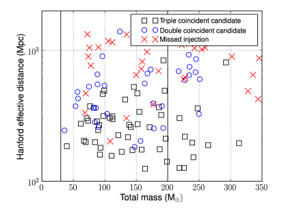
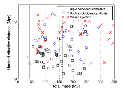
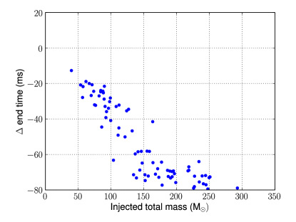
Plots of found and missed injections for the searches are shown in Figure 9. For the most part, simulated signals in the mass range covered by the template banks are well recovered. Some of the missed signals at lower distance correspond to waveforms from simulations of spinning black holes. Since all searches make use of non-spinning waveforms this drop is expected. Finally, we turn to parameter estimation. Figures 10 and 11 show the parameter recovery accuracies for the EOBNR and phenomenological searches respectively. In both cases, the accuracy of recovering the total mass of the simulations is greatly improved over TaylorF2 waveforms shown in Figure 8. This is likely related to the increased mass range of the searches, as well as the use of full waveforms. The timing accuracy for EOBNR is comparable with the TaylorF2 results, while for the phenomenological waveforms, the known timing bias affects the results.
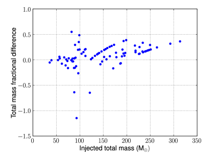
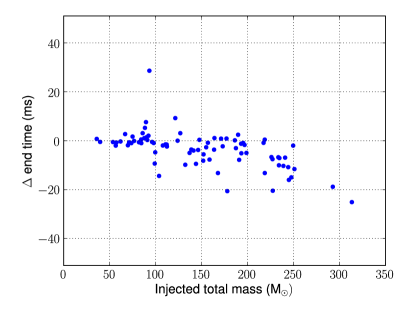
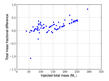
Both the EOBNR and phenomenological models will be improved in the future. Further accurate EOBNR models have already appeared in the literature [65, 68, 69, 70, 71] since the time the EOBNR model used in this analysis was implemented, and extensions to include spin and eccentricity are under development. There are a number of obvious improvements in the phenomenological waveforms that can be made: Calculating the parameter space metric for the phenomenological waveforms would enable the use of an optimal template bank and allow for improved coincidence algorithms. The construction of the phenomenological waveform model can itself be significantly improved by extending the fitting to higher mass ratios and spins, quantifying the error on the phenomenological parameters, matching to post-Newtonian theory as early as possible and including higher order modes in the waveform. The results of the NINJA analysis also demonstrate a clear need to improve accuracy in measuring the end time of the signal. This is not straightforward, however, since there is no clear definition of the time of merger for the phenomenological waveforms or the numerical signals [75]. Work on the improvements to both the EOBNR and phenomenological searches are being made, and will be applied in and guided by future NINJA projects.
4.1.4 Ringdown Templates
As described in section 4.1, ringdown templates can be computed using black hole perturbation theory and so matched filtering can be used to search for these signals. Ringdown templates are exponentially damped sinusoids parametrised by the ringdown frequency and quality factor . The LSC ringdown search pipeline [160] has been used to filter the NINJA data against a bank of ringdown templates with frequencies between 50 Hz and 2 kHz, and quality factors between 2 and 20. The bank had a maximum mismatch of 3% and contained 583 templates. A lower-frequency cutoff of 45 Hz was applied when filtering the NINJA data generated with the LIGO noise curves and 35 Hz for data with the Virgo noise curve. The goals of these analyses were to ascertain the detectability of the injected numerical waveforms using ringdown templates at single and coincident detector levels and the accuracy with which the final black hole parameters can be estimated. The current searches use single-mode templates. The waveforms described in this paper are known to contain higher order multipoles. The potential effects of ignoring these in the search are discussed in Ref. [178] (see in particular Fig. 8 in there).
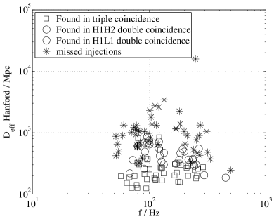
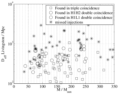
An injection is defined as found if a set of coincident triggers lies within 10 ms of the peak time of the injection (as specified in the contributed numerical data). If more than one set of coincident triggers satisfies this criterion, that with the largest value of is selected, where is the signal to noise ratio in the detector. Of the 126 injections made into the three simulated LIGO detectors, were found in triple coincidence, in H1 and L1 (only), and in H1 and H2 (only). Figure 12 shows the distribution of found and missed injections for this analysis. The ringdown frequency and quality is computed via the Echeverria formulae [179]:
| (12) | |||||
| (13) |
More recent and accurate fits for a variety of modes are listed in the Appendices of Ref. [180]. The final black hole mass and spin can be computed from the component masses and spins of the numerical simulation, as described in [65] and [181], respectively. See also Refs. [51, 182] for a discussion and comparison of different numerical techniques to perform the necessary fits.
As expected, we see that in general, the closest injections (measured by effective distance , defined in equation 10) were found in triple coincidence, those with a large Livingston effective distance were found in H1 and H2 only, while those with a large Hanford effective distance were not found in H2, and the furthest injections were missed in at least two detectors. The plots show that there are three missed injections which, given their frequencies and effective distances, we would have expected to find. However, all three of these are (non-spinning) injections with mass ratio of 4:1, and thus the energy emitted in the ringdown is less than would be emitted by a binary of the same total mass but with a mass ratio of 1 [51]. This is not taken into account in the calculation of effective distance.
Equations (12) and (13) can be
inverted to calculate and from the template parameters and of a given
gravitational-wave candidate. Figure 13 shows the accuracy with
which the ringdown search measures the mass and peak time of the injected
signals. Given that mass is radiated during the ringdown phase (the exact
amount depends on the initial mass ratio) one would expect the measured mass
to underestimate the mass of the signal, and hence the data points would
lie below the diagonal. However, the recovered frequency is systematically
underestimated due to the presence of the preceding inspiral, leading to an
overestimation of the mass. The peak time of the signal is measured with
similar accuracies to the coalescence time measured by the TaylorF2 templates
described in Section 4.1.1. The three data points with a large time
difference and masses lying in the range 80 and 110 are part of the
PU_T52W non-spinning, equal mass group where the peak amplitude
occurred early in the waveform (i.e prior to the merger).
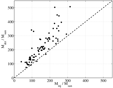
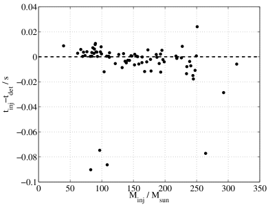
4.2 Search pipelines to detect un-modelled waveforms
Several algorithms exist to detect gravitational wave transients with minimal assumptions on their origin and waveform; these techniques are often referred to as burst searches. Burst searches do not use templates and instead target excesses of power in the time-frequency plane. The LSC and Virgo collaborations have developed several burst search algorithms which use different transformations for the generation of time-frequency data maps. The identification of coherent signatures across multiple detectors has proven to be very effective at suppressing false alarms.
Since they do not assume a template and they target short transients burst searches are suited for the detection of the merger phase of the coalescence. They have the potential to probe a large parameter space, inclusive of spin and ellipticity, at no additional computational cost. For this reason, the NINJA data was analysed by two burst algorithms: Q-pipeline and HHT.
The Q-pipeline [183, 184] is one of the algorithms used in to search for burst sources in LIGO’s fifth science run [185]. It is a multi-resolution time-frequency search for statistically significant excess signal energy, equivalent to a templated matched filter search for sinusoidal Gaussians in whitened data. The template bank is constructed to cover a finite region in central time, central frequency, and quality factor such that the mismatch between any sinusoidal Gaussian in this signal space and the nearest basis function does not exceed a maximum mismatch of 20% in energy. For the purpose of the NINJA analysis, and to explore detectability and parameter estimation, the Q-pipeline analysis was focused on the detection efficiency at the single detector, for all four detectors, using a nominal SNR threshold comparable to the one used in the matched filter searches.
The Hilbert-Huang Transform (HHT) [186, 187] is an adaptive algorithm that decomposes the data into Intrinsic Mode Functions (IMFs), each representing a unique locally monochromatic frequency scale of the data. The original data is recovered by constructing a sum over all IMFs. The Hilbert transform as applied to each IMF unveils instantaneous frequencies and amplitudes as a function of time, thus providing high time-frequency resolution to detected signals without the usual time-frequency-uncertainty as found in basis set methods like the Fourier transform.
In this section we briefly describe how the algorithms were applied and highlight their performance, while Section 4.3 compares the performance of the burst searches to the matched filtering algorithms.
4.2.1 Q-pipeline
The simulated LIGO and Virgo data streams were filtered by the Q-pipeline [210] with the same configuration used in the LSC S5 burst analysis [185]. Data is processed in 64 s analysis blocks with frequency range 48–2048 Hz and Q range 3.3–100. The resulting triggers, once clustered, indicate a time-frequency interval and a significance of the excess power in that time-frequency tile. This significance can be easily converted into the signal-to-noise ratio of a matched filter with sine-Gaussian templates.
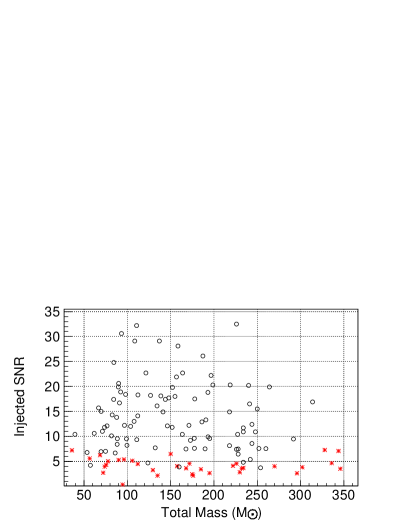
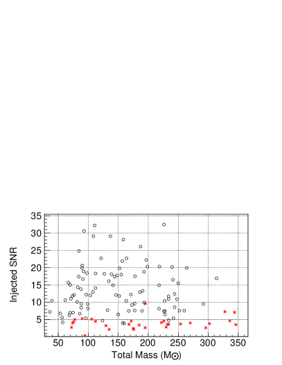
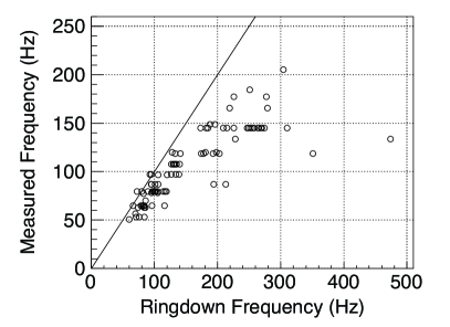
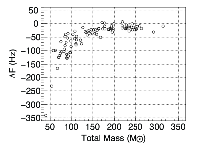
Figure 14 shows the distribution of found and missed injections in the H1 detector as a function of the total mass and the matched filter SNR of the injected waveforms for Q-pipeline (left) and the EOBNR matched filtering search described in section 4.1.3, where both detection thresholds are set at . At the single detector level, the two algorithms have comparable performance. Figure 15 shows the the central frequency of the most significant tile reported by Q-pipeline versus the ringdown frequency computed from equation (12) and the difference between these two frequencies as a function of mass. These results demonstrate that the Q-pipeline preferentially detects the portion of the signal that is in the most sensitive frequency band of the detector (50-200Hz): the ringdown for higher masses, or the inspiral for lower masses.
4.2.2 Hilbert-Huang Transform
An automatic, two-stage HHT pipeline was applied to the NINJA data to detect and characterise the injected signals. Since the HHT pipeline [188] is a new development its application to NINJA data was restricted to the simulated 4 km LIGO detectors H1 and L1. The data was pre-whitened and a Hz low pass zero-phase finite impulse response filter was applied prior to use of the HHT. In the first detection stage, the instantaneous amplitudes from each detector in turn are divided into blocks with similar statistical properties according to the Bayesian Block algorithm [189]. These blocks are then scanned for excess power, with triggered blocks yielding start and end times, thus coincidences between detectors, the maximum frequency, and the signal-to-noise ratio (SNR) of the signal. The second characterisation stage computes the instantaneous frequencies, detailed time-frequency-power maps and time-frequency-power cluster-enhanced maps for the region of data containing the signal identified in the first stage. The overlap of the individual cluster-enhanced maps is used to estimate the time lag between the signals in the detectors and to construct a coherent addition of the two detector data streams used in a final characterisation of the signal.


The excellent resolution of the HHT in time and frequency was used to reject false events due to overly short triggers, failed coincidences or mismatched time-frequency ranges [188]. We identified the latter as a powerful veto tool which could be used to improve the sensitivity of gravitational-wave data analysis pipelines. We were ultimately able to identify 80 events in coincidence, as shown in Figure 16. Three of these candidate events were determined to be false positives when the candidate events were compared to the list of injected signals. Out of the 50 missed events, 39 have injected , five have injected in one detector and in the other, and six had injected in both detectors. We therefore reason that most of the of missed events are low SNR cases in which no blocks were triggered. Most of the cluster-enhanced maps show the time-frequency evolution of the signal with high precision (see Figure 17 for one particular example). Time lag estimates and coherent additions show strong potential and can be seen as proof of principle, but need further refinement to work reliably in an automatic pipeline. SNR estimates are difficult since only the burst region or diverse fragments of the signal are visible in our search. We refer to [190] for further details of this analysis.
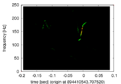
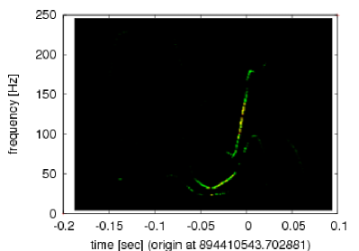
4.3 Comparison of Inspiral-Burst-Ringdown Results
In this section we consider comparisons between several of the search pipelines described in the preceding sections. The performance of a pipeline depends on many parameters, such as the signal-to-noise thresholds, the trigger coincidence and coherence tests, signal-based vetoes tests, allowed false alarm rates, etc. Search pipelines are tuned to suppress false alarms while preserving detection efficiency and tuning decisions can dramatically affect the relative performance of one pipeline versus another. Given the limited scope of the NINJA data set, a comprehensive comparison of pipelines was not possible. However, to make a first-order comparison between search pipelines applied to the NINJA data, disentangled from pipeline tuning decisions, we compared the number of injections found in a single detector at a fixed matched-filter signal-to-noise threshold.
Table 8 reports the number of injections found in single interferometers and in multi-interferometer networks, using triggers from the Q-pipeline burst algorithm (which targets the merger by match filtering to sine-Gaussian templates), matched filter to ringdown templates, matched filter to inspiral templates and matched filter to non-spinning, full coalescence EOBNR waveforms. For all algorithms the same nominal threshold of was imposed. In addition, the number of detected injections in AND (injections detected simultaneously from multiple algorithms) and OR (injections detected by at least one algorithm) in an inspiral-merger-ringdown analysis is reported.
The statistics of this sample is too small to make inferences on which pipeline performs better in which parameter region; a more systematic study is needed. Furthermore, since the NINJA data contains only Gaussian noise and signals and so this comparison does not take into account noise transients which may cause false detections. Nevertheless, we have an indication that all pipelines have comparable chances to find these injections. The differences between pipelines are in the accuracy with which they can measure the parameters of the signal.
| H1 | H2 | L1 | V1 | H1L1 | H1H2L1 | H1L1V1 | H1H2L1V1 | |
| 94 | 60 | 93 | 105 | 84 | 58 | 68 | 48 | |
| Q-pipeline (M) | 88 | 55 | 85 | 92 | 77 | 51 | 57 | 40 |
| Ringdown (R) | 88 | 56 | 83 | 93 | 76 | 52 | 56 | 40 |
| M-R AND | 87 | 55 | 82 | 91 | 76 | 51 | 56 | 40 |
| M-R OR | 89 | 56 | 86 | 94 | 77 | 52 | 57 | 40 |
| TaylorF2 (I) | 85 | 43 | 82 | – | 75 | 43 | – | – |
| I-M-R AND | 82 | 42 | 77 | – | 72 | 41 | – | – |
| I-M-R OR | 91 | 57 | 88 | – | 80 | 55 | – | – |
| EOBNR (E) | 90 | 56 | 88 | 100 | 79 | 54 | 64 | 45 |
| E-M-R AND | 86 | 53 | 81 | 88 | 75 | 49 | 56 | 39 |
| E-M-R OR | 92 | 58 | 91 | 104 | 81 | 56 | 65 | 47 |
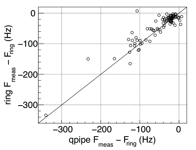
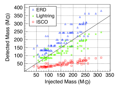
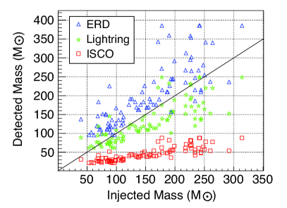
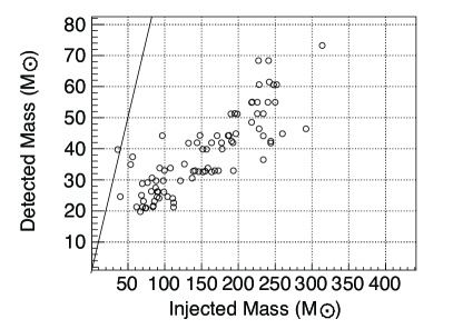
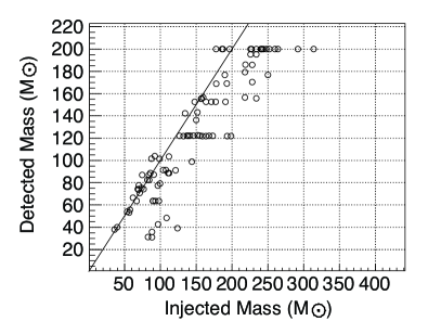
Figure 18 compares the accuracy with the Q-pipeline and ringdown searches measure the frequency of the signal and Figures 19 compares the accuracy with these pipelines measure the total mass of the injected signal. Both the ringdown and Q-pipeline searches report a frequency not a mass, so to compare to the injected and detected total masses we must calculate a mass from the frequency of the candidate. There is no unique way to do this, and but we can calculate the total mass under the assumption the algorithm is detecting a given portion of the waveform. Figure 19 shows the result of using the formulae for ISCO, light-ring and effective ringdown frequencies to compute the total mass [64, 173]:
| (14) |
Both burst and ringdown code preferentially detect the portion of the signal that is in the detectors’ most sensitive band. Figure 19 shows that for both algorithms, at the lowest injected masses this correspond to , but as the injected mass increases, the algorithms trigger between light ring and ringdown, as expected.
This comparison is more straightforward for matched filtering codes that use a template with a given mass. Figure 20 shows the detected total mass against the injected total mass for (i) 2.0 post-Newtonian order TaylorF2 templates terminated at , with templates in the mass range 20–90 M⊙ and (ii) EOBNR templates with masses in the range to 30–200 M⊙. The TaylorF2 templates significantly underestimate the masses of the injected signals, due to the fact that most of the injected signals lie outside the template bank. The EOBNR search, with its larger mass range and inspiral-merger-ringdown waveforms, measures the masses of the injected signals with better accuracy.
4.4 Bayesian pipelines
Bayesian inference [191] is a powerful means of extracting information from observational data based on the calculation of posterior probabilities and probability density functions. Computation of these quantities is expensive and so these algorithms are not typically used to search for candidate events in detector data. They are, however, useful in the closer study of candidates identified by the search pipelines described in Sections 4.1 and 4.2. This section describes the results of applying two different Bayesian inference algorithm to the NINJA data. The first is designed to estimate the parameters of the signal assuming a gravitational wave is present in the data. The second calculates the confidence in the presence of the signal, quantified by the odds ratio between the signal and noise models of the data.
Both approaches require the calculation of the posterior probability-density function (PDF) on the parameter space of the signal, given the data , which is
| (15) | |||||
in the presence of Gaussian noise with power spectral density , where is the prior probability density of the parameters and is the model used to describe the signal [192].
A Markov-Chain Monte-Carlo approach [193] was used to coherently analyse data from multiple detectors in order to evaluate the posterior PDFs. This technique stochastically samples the parameter space in a search for the parameters that best match the observed data; it does so by attempting a random jump from the current set of parameter values to a new one, then deciding whether the jump should be taken by comparing the likelihoods of the old and new locations in parameter space. In this way, one simultaneously searches for the set of parameters that yield the best fit to the data, and determines the accuracy of the parameter estimation.
Bayesian model selection, based on a different Monte-Carlo technique known as nested sampling [194], was employed as a tool to measure the confidence of a detection using different waveform families. This approach requires the calculation of the marginal likelihood of the signal and noise models, obtained by computing the integral of the posterior PDF to find the total probability of the model. It was possible to calculate this integral for the nine-parameter model of a non-spinning binary coalescence signal described coherently in multiple interferometers. The ratio of likelihoods of the signal and noise models is known as the “Bayes factor,” and is used to multiply prior odds, giving the posterior odds ratio between the two models, taking into account the observational data; in turn, the value of this Bayes factor corresponds to the level of confidence in the detection. As a straightforward by-product of the nested-sampling algorithm, it is also possible to infer the maximum-likelihood values of the parameters of the detected signals; this was used to obtain further information on the ability of different waveform approximants to recover the source parameters.
4.4.1 Parameter Estimation Using Markov Chain Monte Carlo
A selection of injected numerical signals were analysed with a Markov-Chain Monte Carlo (MCMC) code [195, 196]. The signal model was based on waveforms with phase evolution at 1.5 post-Newtonian order and leading-order amplitude evolution. Parameter estimation was successful on NINJA injections with relatively low total mass in which the inspiral contained a significant fraction of the total signal-to-noise ratio. For high-mass injections, the algorithm attempted to match the merger and ringdown portions of the injected signal to inspiral templates, resulting in poor parameter estimation.
The post-Newtonian waveforms used in this analysis include the spin of the larger body , allowing us to use the analytical simple-precession waveform [197]. The parameter space thus consists of twelve independent parameters:
| (16) |
where and are the chirp mass and symmetric mass ratio, respectively; (right ascension) and (declination) identify the source position in the sky; the angles and identify the direction of the total angular momentum of the binary; is the luminosity distance to the source; is the dimensionless spin magnitude; is the cosine of the angle between the spin and the orbital angular momentum; and and are integration phase constants that specify the gravitational-wave phase and the location of the spin vector on the precession cone, respectively, at the time of coalescence .
The MCMC algorithm used for the NINJA analysis was optimised by including a variety of features to efficiently sample the parameter space, such as parallel tempering [196]. This MCMC implementation can be run on a data set from a single detector, or on data sets from multiple detectors. In the latter case, a coherent search among all detectors significantly improves the determination of source position and orientation [195, 196].
The MCMC code was run on a selection of injected signals in the NINJA data. It was found that although the MCMC runs are clearly able to detect a signal whenever the inspiral contains a sufficient signal-to-noise ratio (SNR), they were unable to correctly determine the signal parameters for many injections. For the high masses typical of most NINJA injections, the SNR is dominated by the merger and ringdown, so that the inspiral-only templates tried to match the merger and ringdown portions of the injected waveform. Typically, it is found that in such cases the time of coalescence is overestimated since the injected ringdown is matched to an inspiral; the chirp mass is underestimated since the merger/ringdown frequency is higher than the inspiral frequency for a given mass, so that matching them to an inspiral requires the mass to be lower; the mass ratio is underestimated, which allows the waveform to contain more energy in the narrow frequency band corresponding to quasi-normal ringing; and the spin rails against the upper prior of since the innermost stable circular orbit frequency is highest for an inspiral into a maximally-spinning Kerr black hole. We tried to circumvent the problem of matching to the merger and ringdown by introducing more-restrictive priors on spin and/or . These efforts still failed when the total masses were too high, but were successful in the case of lower total masses and longer inspiral signals.


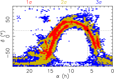
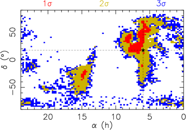
Figure 21 shows the PDFs produced by runs on an injected equal-mass non-spinning SpEC Cornell/Caltech waveform with . This particular injection was chosen because it had the lowest total mass, and SpEC waveforms typically have more inspiral cycles; runs on other injections show comparable results, with the general trend that the higher the total mass (and, thus, the lower the relative fraction of the SNR contributed by the inspiral), the poorer the parameter estimation becomes.
Data from two detectors, H1 and L1, were used to compute the PDFs shown in the top row of Figure 21. We used wide, flat priors for intrinsic parameters (e.g., , , ). We find that the values of the intrinsic parameters are not determined very accurately. In particular, the spin rails against the upper bound of while is underestimated, as expected. We find that the sky location is nevertheless constrained to an arc of a ring containing the true value; the 2- (%) sky area of the ring shown in the bottom left of Fig. 21 is square degrees.
In the middle row of Fig. 21, we plot the PDFs based on data from three detectors: H1, L1, and V1. The spin parameter was constrained to its true value for this run. This had the effect of forcing the MCMC to match the inspiral only, significantly improving the resolution of other parameters: for example, the PDF of now rails against , which is its true value. The chirp mass is still somewhat underestimated; a higher SNR may be necessary to improve the mass determination. Promisingly, it was found that the sky location is constrained to a smaller patch on the sky: the 2- sky area in the bottom right of Fig. 21 is square degrees. In fact, the sky localisation is even better when the spin parameter is allowed to vary, allowing the MCMC to use the SNR contributed by the ringdown; removing the spin-parameter constraint reduces the 2- sky area to square degrees. This ability to determine the source position will be significant in any future searches for electromagnetic counterparts of gravitational-wave triggers.
We hope that in the future it will be possible to test MCMC codes on numerical signals in a lower mass range, where the inspiral portion would dominate the SNR, so that inspiral-only templates are not at a significant disadvantage. Meanwhile, we have recently implemented templates at 3.5 PN order in phase that include the spin for both members of the binary, thus improving the accuracy of parameter estimation and increasing the range of applicability of our code.
4.4.2 Bayesian Model Selection Pipeline
The primary goal of this analysis was to investigate the performance of different template families on the confidence of detection of the injections contained in the NINJA data set. The approach to this problem used a method described in [198, 199], which can be summarised as follows. Two hypotheses are under consideration: (i) —The data are described by (Gaussian and stationary) noise only: , and (ii) —The data are described by (Gaussian and stationary) noise and a gravitational wave signal , according to a given approximant , where represents the vector of the (unknown) signal parameters: . The marginal likelihood of is calculated by performing the integral
| (17) |
The ratio of probabilities or “odds ratio” of the two models is
| (18) | |||||
where is the prior odds ratio and is the Bayes factor.
In this analysis the model includes the response of all available simulated detectors (L1, H1, H2 and V1) coherently, and the gravitational waveforms are calculated using function in the LAL library [149]. For the gravitational waveform, two different approximants were considered: the standard (2 PN) TaylorF2 waveform family, with inspiral truncated at , and the phenomenological inspiral-merger-ringdown IMRPhenA templates described in [63]. In each case the waveforms were truncated at low frequency at 30 Hz.
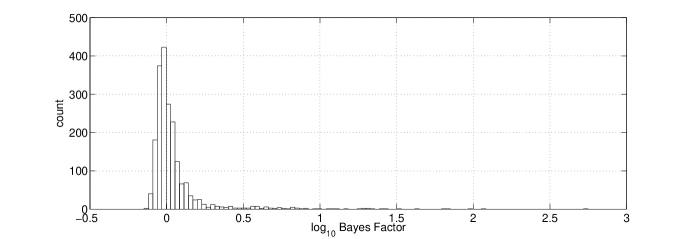
The choice of priors in the analysis was as follows. For the TaylorF2 approximant, the prior on was uniform on chirp mass, symmetric mass ratio and distance, within the following limits: time of coalescence in a window s around the actual of each injection, symmetric mass ratio in the range , chirp mass within the bounds set by and the total mass in the range , and distance Mpc. The parameters for orientation and position on the sky of the binary were allowed to vary over their entire angular ranges. For the IMRPhenA approximant, the limits were identical on all the parameters, with the exception of the total mass whose upper boundary was set to . We also calculated the Bayes factors for data segments containing no signal in order to estimate the background distribution of Bayes factors. Figure 22 shows the distribution of Bayes factors (using TaylorF2 approximants) when running the analysis algorithm on portions of data without injections: 2000 trials were carried out, with a maximum value of . If interpreted as a threshold value on the Bayes factors to decide whether a signal has been detected or not, it corresponds to a false alarm of . The distribution obtained with the IMRPhenA approximant is very similar. In the analysis, a range of “detection thresholds” on was considered, in order to explore how the two different approximants (and the algorithm) respond to different numerical relativity injections.
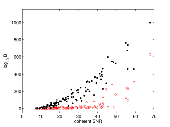
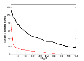
Figure 23 and Table 9 summarise the main results. The left panel of Figure 23 shows the value of the Bayes factor computed for the two approximants as a function of the coherent four-detector signal-to-noise ratio at which the waveforms were injected. For all the injections, IMRPhenA approximants return a Bayes factor which is (significantly) larger than TaylorF2 approximants. This is not surprising, as the TaylorF2 waveforms do not contain the merger and ring-down portion of the coalescence and are truncated at . Figure 23 (right panel) shows the number of injections that are recovered at a given Bayes factor (or above). Once more the effectiveness of IMRPhenA approximants is striking compared to the TaylorF2 waveform family. These results are broadly in agreement with the matched-filter analysis carried out with inspiral-merger-ringdown waveforms described in Section 4.1.3.
| Threshold | Number of detected injections | |
|---|---|---|
| ) | TaylorF2 | IMRPhenA |
| 3 | 69 | 112 |
| 5 | 61 | 107 |
| 10 | 43 | 104 |
| 30 | 28 | 89 |
| 100 | 10 | 58 |
The nested-sampling algorithm used for model-selection can also be used for parameter estimation. In particular, one can generate in a straightforward way the maximum likelihood estimate of the recovered parameters, and have an indication of the statistical errors on such values. For simplicity, in this analysis we identified the statistical errors (the error bars in Figures 24 and 25) with the region of parameter space in which the likelihood values were not lower than a factor with respect to the maximum likelihood. The results for chirp mass, total mass and the two coordinates of the source in the sky – latitude and longitude – are shown in Figures 24 and 25; here we restrict to only the IMRPhenA approximant and to all the signals that yielded . The results for the masses show a behaviour that is qualitatively consistent with the results obtained using a matched-filtering analysis, see e.g. Figures 10, 11, and 20. The total mass is (in most of the cases) systematically underestimated, although for 34 injections the recovered values were consistent with the injected total mass. These injections correspond in all cases to waveforms with (near) zero eccentricity and in 21 (out of 34) instances to non-spinning waveforms. We have also checked that the errors on the masses do not show any significant correlation with the value of the Bayes factor at which the injections were recovered or the injected signal-to-noise ratio. However, despite the systematic errors on the physical parameters, the sky location is on average fairly well determined. This is most likely due to the fact that there is enough information in the (source-location dependent) time of arrival of the signals at different instrument sites to recover meaningful information about the position of the source in the celestial sphere. This is currently under careful investigation and more details about this and other aspects of the analysis can be found in Ref. [200].
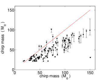
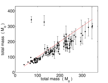
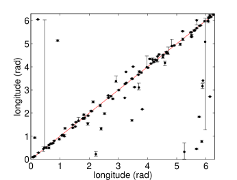
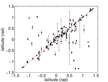
5 Conclusion
The NINJA project was conceived as a first step towards a long-term collaboration between numerical relativists and data analysts with the goal of using numerical waveforms to enhance searches for gravitational waves. NINJA is unique in that it focused on running existing gravitational-wave search algorithms on data containing waveforms obtained from numerical simulations. Since this constitutes the first such analysis, the scope of the project was deliberately kept somewhat modest: restrictions were placed on the number of waveforms to be submitted by each numerical group, no attempt was made to include transient noise sources in the data and only a limited number of simulated signals were produced for the data analysis. This helped to encourage significant involvement from both the numerical relativity and data analysis communities, with ten numerical relativity groups providing waveforms and data-analysis contributions from nine different groups.
Communication between the data analysis and numerical communities has been smooth and fluent during the course of the NINJA project. The format described in [76] provided a good starting point from which to interchange data between the communities. As the project was being developed, several improvements were made to the format, which we expect will continue evolving as more experience is gained with a broader family of waveforms, including those containing matter.
The limited number of signals in the NINJA data makes it dangerous to draw strong conclusions from the comparison of different waveform families and different search methods. Overall, it is clear that many of the data analysis methods were capable of detecting a significant fraction of the simulated waveforms. This is immediately significant as several of the analyses performed are routinely used in searches of the LIGO and Virgo data. However, since the NINJA data set did not include the type of non-Gaussian transients seen in real gravitational-wave detector data, it is difficult to translate the efficiencies observed here into statements about LIGO or Virgo sensitivity.
NINJA has demonstrated that more work is required to measure the parameters of signals in detector data. Parameter estimation is poor for most pipelines, and several methods tend to associate a candidate event to that part of the waveform which lies in the most sensitive band of the detector. For example, in a search with inspiral only templates, the ringdown of a high mass black hole which occurs at around 100 Hz might be picked up. This will lead to poor estimation of both the binary’s mass and coalescence time. Similarly, the un-modelled burst searches will correctly identify the signal but, without knowing which part of the coalescence it corresponds to, have difficulty providing accurate parameters. There is some evidence that using full inspiral-merger-ringdown waveform templates alleviates this problem, as well as evidence that estimation of the sky location of the signal is largely independent of the mismatches between simulated and template waveform. These are all issues which warrant further investigation.
We hope that this work will provide a foundation for future analyses, and plans are envisioned to continue and extend the NINJA project. Several suggestions have been made to broaden this work and make it more systematic: in addition to expanding the parameter space explored by numerical simulations, two crucial steps will be to construct hybrid analytic-numerical waveforms (which will allow a lower range of masses to be injected) and to consider data containing non-stationary noise. It would also be natural to include other waveform families, such as supernovae or binary mergers comprising one or two neutron stars. Subsequent NINJA projects could provide a noise-free data set for tuning parameter estimation and measurement pipelines and release “training” and “challenge” data sets, as has proven successful in the Mock LISA Data Challenges [201, 202], in which the parameters of the waveforms are known and unknown to the analysts, respectively. The numerical data sets may also be useful for efforts aimed at using the best-available waveforms to explore and develop LISA data analysis approaches and in evaluating parameter estimation accuracy for LISA. These efforts, as carried out by the Mock LISA Data Challenge Task Force and the LISA Parameter Estimation Task Force, are summarised in Ref. [203, 204].
However future analyses progress, it is clear that a significant amount remains to be learned from collaborations between the numerical relativity and gravitational-wave data analysis communities.
Acknowledgements
We thank Alan Weinstein for helpful comments on this paper and the Kavli Institute for Theoretical Physics (KITP) Santa Barbara for hospitality during the workshop “Interplay between Numerical Relativity and Data Analysis,” where the NINJA project was initiated. The Kavli Institute is supported by National Science Foundation grant PHY-0551164.
This project was supported in part by DFG grant SFB/Transregio 7 “Gravitational Wave Astronomy” (BB, MH, SH, DP, LR, US); by National Science Foundation grants PHY-0114375 (CGWP), PHY-0205155 (UIUC), PHY-0354842 (RM), DMS-0553302 (MB, LB, TC, KM, HP, MS), DMS-0553677 (LK, AM), PHY-0553422 (NC), PHY-0555436 (PL), PHY-0600953 (PB, LG, RAM, RV), PHY-0601459 (MB, LB, TC, KM, HP, MS), PHY-0603762 (AB, EO, YP), PHY-0649224 (BF), PHY-0650377 (UIUC), PHY-0652874 (FAU), PHY-0652929 (LK, AM), PHY-0652952 (LK, AM), PHY-0652995 (MB, LB, TC, KM, HP, MS), PHY-0653303 (PL, DS, MC, CL), PHY-0653321 (VK, IM, VR, MvdS), PHY-0653443 (DS), PHY-0653550 (LC), PHY-0701566 (ES), PHY-0701817 (PB, LG, RAM, RV), PHY-0714388 (MC, CL, YZ), OCI-0721915 (ES), PHY-0722315 (MC, CL), PHY-0745779 (FP), PHY-0801213 (FH), PHY-0838740 (BF, LS, VR) and NSF-0847611 (DB, LP); by NASA grants HST-AR-11763 (CL, MC, JF, YZ), NNG-04GK54G (UIUC), NNG-04GL37G (RM), NNG-05GG51G (LK, AM), NNG-05GG52G (MB, LB, TC, KM, HP, MS), 05-BEFS-05-0044 (GSFC), 06-BEFS06-19 (GSFC), 07-ATFP07-0158 (MC, CL, YZ), and NNX-07AG96G (UIUC), and by NSF cooperative agreement PHY-0107417 (DK, SC).
BA was supported by a Vacation Bursary of the UK Engineering and Physical Sciences Research Council. AV, JV and BS acknowledge support by the UK Science and Technology Facilities Council. SF acknowledges the support of the Royal Society. MH was supported by SFI grant 07/RFP/PHYF148. FP acknowledges support from the Alfred P. Sloan Foundation. SH acknowledges support from DAAD grant D/07/13385, grant FPA-2007-60220 from the Spanish Ministry of Science and Education and VESF. MB, LB, TC, KM, HP and MS acknowledge support from the Sherman Fairchild Foundation and the Brinson Foundation. LK and AM acknowledge support from the Fairchild Foundation. BK was supported by the NASA Postdoctoral Program at the Oak Ridge Associated Universities. SM was supported in part by the Leon A. Herreid Graduate Fellowship. RS was supported by an EGO sponsored fellowship, EGO-DIR-105-2007.
Computations were carried out under LRAC allocations MCA08X009 (PL, DS), TG-MCA08X010 (FAU), TG-MCA02N014 (LSU), TG-MCA99S008 (UIUC), TG-PHY990002 (MB, LB, TC, LK, KM, AM, HP, MS), on LONI systems (LSU), and on the clusters at the AEI, Cardiff University, Northwestern University (NSF MRI grant PHY-0619274 to VK), the LIGO Laboratory, NASA Advanced Supercomputing Division (Ames Research Center), Syracuse University, LRZ Munich (BB, MH, SH, US), the University of Birmingham, and the RIT NewHorizons cluster.
Appendix A Glossary of terms
| Term | Meaning |
|---|---|
| ADM | Arnowitt-Deser-Misner. |
| ASCII | American Standard Code for Information Interchange. |
| BAM | Bifunctional Adaptive Mesh code developed at University of Jena. |
| BBH | Binary Black Hole. |
| BSSN | Baumgarte-Shapiro-Shibata-Nakamura 3+1 formulation of |
| Einstein’s equations. | |
| CBC | Compact Binary Coalescence. |
| CCATIE | AEI/LSU numerical relativity code. |
| EOB | Effective One Body. |
| EOBNR | Effective-one-body waveforms calibrated to numerical data. |
| ERD | Effective Ringdown. |
| GH | Generalized harmonic formulation of Einstein’s equations. |
| Hahndol | Numerical-relativity code developed at NASA-Goddard. |
| HHT | Hilbert-Huang Transform. |
| IMF | Intrinsic Mode Functions. |
| IMR | Inspiral-Merger-Ringdown. |
| ISCO | Innermost Stable Circular Orbit. |
| L1, H1, H2, V1 | LIGO Livingston 4 km, Hanford 4 km, Hanford 2 km |
| and Virgo 3 km gravitational-wave detectors. | |
| LAL | LSC Algorithm Library. |
| Lean | Numerical-relativity code developed by Ulrich Sperhake. |
| LazEv | Brownsville/RIT numerical relativity code. |
| LSC | LIGO Scientific Collaboration. |
| MayaKranc | Numerical-relativity code developed at Penn State |
| using the Kranc code-generation package developed at AEI, | |
| Southampton and Penn State. | |
| MCMC | Markov-Chain Monte-Carlo. |
| NINJA | Numerical INJection Analysis. |
| NR | Numerical Relativity. |
| Probability-density Function. | |
| PN | Post-Newtonian. |
| PU | Numerical-relativity code developed by Frans Pretorius. |
| S5 | Fifth LIGO science run. |
| SNR | Signal-to-noise ratio. |
| SPA | Stationary Phase Approximation. |
| SpEC | Spectral Einstein Code developed at Caltech and Cornell. |
| TT | Transverse-Traceless. |
| UIUC | University of Illinois at Urbana-Champagn numerical |
| relativity code. | |
| VSR1 | Virgo science run 1. |
| WRD | Weighted ringdown. |
References
References
- [1] Thorne K S 1987 Three hundred years of gravitation ed Hawking S W and Israel W (Cambridge: Cambridge University Press) chap 9, pp 330–458
- [2] Einstein A 1916 Preuss. Akad. Weiss. Berlin 688
- [3] Peters P C and Mathews J 1963 Phys. Rev. 131 435–439
- [4] Peters P C 1964 Phys. Rev. 136 B1224–B1232
- [5] Barish B C and Weiss R 1999 Phys. Today 52 44–50
- [6] Acernese F et al. (VIRGO) 2005 AIP Conf. Proc. 794 307–310
- [7] Tsubono K (TAMA) 2002 Rome 2000, Recent developments in theoretical and experimental general relativity, gravitation and relativistic field theories, Pt. A ed VG Gurzadyan R J and Ruffini R (Singapore: World Scientific) pp 145–154 prepared for 9th Marcel Grossmann Meeting on Recent Developments in Theoretical and Experimental General Relativity, Gravitation and Relativistic Field Theories (MG 9), Rome, Italy, 2-9 Jul 2000
- [8] Willke B (LIGO Scientific) 2007 Class. Quant. Grav. 24 S389–S397
- [9] Abbott B et al. (LIGO Scientific) 2004 Nucl. Instrum. Meth. A 517 154–179 (Preprint gr-qc/0308043)
- [10] Abbott B et al. (LIGO Scientific) 2007 LIGO: The Laser Interferometer Gravitational-Wave Observatory (Preprint 0711.3041)
- [11] Acernese F et al. 2008 J. Phys. Conf. Ser. 120 032007
- [12] Uchiyama T et al. 2004 Class. Quant. Grav. 21 S1161–S1172
- [13] Abbott B et al. (LIGO Scientific) 2009 Search for Gravitational Waves from Low Mass Binary Coalescences in the First Year of LIGO’s S5 Data (Preprint 0901.0302)
- [14] Abbott B et al. (LIGO Scientific) 2004 Phys. Rev. D 69 122001 (Preprint gr-qc/0308069)
- [15] Abbott B et al. (LIGO Scientific) 2005 Phys. Rev. D 72 082001 (Preprint gr-qc/0505041)
- [16] Abbott B et al. (LIGO Scientific) 2005 Phys. Rev. D 72 082002 (Preprint gr-qc/0505042)
- [17] Abbott B et al. (LIGO Scientific) 2008 Phys. Rev. D 77 062002 (Preprint 0704.3368)
- [18] Abbott B et al. (LIGO Scientific) 2008 Phys. Rev. D 78 042002 (Preprint 0712.2050)
- [19] Abbott B et al. (LIGO Scientific) 2004 Phys. Rev. D 69 102001 (Preprint gr-qc/0312056)
- [20] Abbott B et al. (LIGO Scientific) 2005 Phys. Rev. D 72 062001 (Preprint gr-qc/0505029)
- [21] Abbott B et al. (LIGO Scientific) 2006 Class. Quant. Grav. 23 S29–S39 (Preprint gr-qc/0511146)
- [22] Abbott B et al. (TAMA) 2005 Phys. Rev. D 72 122004 (Preprint gr-qc/0507081)
- [23] Abbott B et al. (LIGO Scientific) 2007 Class. Quant. Grav. 24 5343–5370 (Preprint 0704.0943)
- [24] Pretorius F 2005 Phys. Rev. Lett. 95 121101 (Preprint gr-qc/0507014)
- [25] Campanelli M, Lousto C O, Marronetti P and Zlochower Y 2006 Phys. Rev. Lett. 96 111101 (Preprint gr-qc/0511048)
- [26] Baker J G, Centrella J, Choi D I, Koppitz M and van Meter J 2006 Phys. Rev. Lett. 96 111102 (Preprint gr-qc/0511103)
- [27] Pretorius F 2009 Physics of Relativistic Objects in Compact Binaries: from Birth to Coalescence ed Colpi M, Casella P, Gorini V, Moschella U and Possenti A (Heidelberg, Germany: Springer) (Preprint 0710.1338)
- [28] Husa S 2007 Eur. Phys. J. ST 152 183–207 (Preprint 0812.4395)
- [29] Hannam M 2009 Status of black-hole-binary simulations for gravitational-wave detection (Preprint 0901.2931)
- [30] Herrmann F, Hinder I, Shoemaker D and Laguna P 2007 Class. Quant. Grav. (Preprint gr-qc/0601026)
- [31] Baker J G et al. 2006 Astrophys. J. 653 L93–L96 (Preprint astro-ph/0603204)
- [32] Gonzalez J A, Sperhake U, Brügmann B, Hannam M and Husa S 2007 Phys. Rev. Lett. 98 091101 (Preprint gr-qc/0610154)
- [33] Herrmann F, Hinder I, Shoemaker D, Laguna P and Matzner R A 2007 Astrophys. J. 661 430–436 (Preprint gr-qc/0701143)
- [34] Koppitz M et al. 2007 Phys. Rev. Lett. 99 041102 (Preprint gr-qc/0701163)
- [35] Campanelli M, Lousto C O, Zlochower Y and Merritt D 2007 Astrophys. J. 659 L5–L8 (Preprint gr-qc/0701164)
- [36] Gonzalez J A, Hannam M D, Sperhake U, Brügmann B and Husa S 2007 Phys. Rev. Lett. 98 231101 (Preprint gr-qc/0702052)
- [37] Tichy W and Marronetti P 2007 Phys. Rev. D 76 061502 (Preprint gr-qc/0703075)
- [38] Campanelli M, Lousto C O, Zlochower Y and Merritt D 2007 Phys. Rev. Lett. 98 231102 (Preprint gr-qc/0702133)
- [39] Baker J G et al. 2007 Astrophys. J. 668 1140–1144 astro-ph/0702390
- [40] Herrmann F, Hinder I, Shoemaker D M, Laguna P and Matzner R A 2007 Phys. Rev. D 76 084032 (Preprint 0706.2541)
- [41] Brügmann B, Gonzalez J A, Hannam M, Husa S and Sperhake U 2008 Phys. Rev. D 77 124047 (Preprint 0707.0135)
- [42] Schnittman J D et al. 2008 Phys. Rev. D 77 044031 (Preprint 0707.0301)
- [43] Pollney D et al. 2007 Phys. Rev. D 76 124002 (Preprint 0707.2559)
- [44] Lousto C O and Zlochower Y 2008 Phys. Rev. D 77 044028 (Preprint 0708.4048)
- [45] Baker J G et al. 2008 Astrophys. J. 682 L29 (Preprint 0802.0416)
- [46] Dain S, Lousto C O and Zlochower Y 2008 Phys. Rev. D 78 024039 (Preprint 0803.0351)
- [47] Healy J et al. 2008 Superkicks in Hyperbolic Encounters of Binary Black Holes (Preprint 0807.3292)
- [48] Gonzalez J A, Sperhake U and Brügmann B 2008 Black-hole binary simulations: the mass ratio 10:1 (Preprint 0811.3952)
- [49] Campanelli M, Lousto C O and Zlochower Y 2006 Phys. Rev. D 74 084023 (Preprint astro-ph/0608275)
- [50] Campanelli M, Lousto C O, Zlochower Y, Krishnan B and Merritt D 2007 Phys. Rev. D 75 064030 (Preprint gr-qc/0612076)
- [51] Berti E et al. 2007 Phys. Rev. D 76 064034 (Preprint gr-qc/0703053)
- [52] Rezzolla L et al. 2008 Astrophys. J. 679 1422–1426 (Preprint 0708.3999)
- [53] Boyle L, Kesden M and Nissanke S 2008 Phys. Rev. Lett. 100 151101 (Preprint 0709.0299)
- [54] Rezzolla L et al. 2008 Astrophys. J. 674 L29–L32 (Preprint 0710.3345)
- [55] Marronetti P, Tichy W, Brügmann B, Gonzalez J and Sperhake U 2008 Phys. Rev. D 77 064010 (Preprint 0709.2160)
- [56] Sperhake U et al. 2008 Phys. Rev. D 78 064069 (Preprint 0710.3823)
- [57] Hinder I, Vaishnav B, Herrmann F, Shoemaker D and Laguna P 2008 Phys. Rev. D 77 081502 (Preprint 0710.5167)
- [58] Berti E, Cardoso V, Gonzalez J A, Sperhake U and Brügmann B 2008 Class. Quant. Grav. 25 114035 (Preprint 0711.1097)
- [59] Boyle L and Kesden M 2008 Phys. Rev. D 78 024017 (Preprint 0712.2819)
- [60] Tichy W and Marronetti P 2008 Phys. Rev. D 78 081501 (Preprint 0807.2985)
- [61] Rezzolla L 2009 Class. Quant. Grav. 26 094023 (Preprint 0812.2325)
- [62] Buonanno A, Cook G B and Pretorius F 2007 Phys. Rev. D 75 124018 (Preprint gr-qc/0610122)
- [63] Ajith P et al. 2008 Phys. Rev. D 77 104017 (Preprint 0710.2335)
- [64] Pan Y et al. 2008 Phys. Rev. D 77 024014 (Preprint 0704.1964)
- [65] Buonanno A et al. 2007 Phys. Rev. D 76 104049 (Preprint 0706.3732)
- [66] Boyle M et al. 2007 Phys. Rev. D 76 124038 (Preprint 0710.0158)
- [67] Ajith P et al. 2007 Class. Quant. Grav. 24 S689–S700 (Preprint 0704.3764)
- [68] Damour T and Nagar A 2008 Phys. Rev. D 77 024043 (Preprint 0711.2628)
- [69] Damour T, Nagar A, Dorband E N, Pollney D and Rezzolla L 2008 Phys. Rev. D 77 084017 (Preprint 0712.3003)
- [70] Damour T, Nagar A, Hannam M, Husa S and Brügmann B 2008 Phys. Rev. D 78 044039 (Preprint 0803.3162)
- [71] Boyle M et al. 2008 Phys. Rev. D 78 104020 (Preprint 0804.4184)
- [72] Boyle M, Brown D A and Pekowsky L 2009 Class. Quant. Grav. 26 114006 (Preprint 0901.1628)
- [73] Baumgarte T et al. 2008 Phys. Rev. D 77 084009 (Preprint gr-qc/0612100)
- [74] Vaishnav B, Hinder I, Herrmann F and Shoemaker D 2007 Phys. Rev. D 76 084020 (Preprint 0705.3829)
- [75] Hannam M et al. 2009 Phys. Rev. D 79 084025 (Preprint 0901.2437)
- [76] Brown D A et al. 2007 Data formats for numerical relativity waves (Preprint 0709.0093)
- [77] Brügmann B et al. 2008 Phys. Rev. D 77 024027 (Preprint gr-qc/0610128)
- [78] Husa S, Gonzalez J A, Hannam M, Brügmann B and Sperhake U 2008 Class. Quant. Grav. 25 105006 (Preprint 0706.0740)
- [79] Hannam M, Husa S, Sperhake U, Brügmann B and Gonzalez J A 2008 Phys. Rev. D 77 044020 (Preprint 0706.1305)
- [80] Hannam M, Husa S, Brügmann B and Gopakumar A 2008 Phys. Rev. D 78 104007 (Preprint 0712.3787)
- [81] Brügmann B, Tichy W and Jansen N 2004 Phys. Rev. Lett. 92 211101 (Preprint gr-qc/0312112)
- [82] Alcubierre M et al. 2000 Phys. Rev. D 62 044034 (Preprint gr-qc/0003071)
- [83] Alcubierre M et al. 2003 Phys. Rev. D 67 084023 (Preprint gr-qc/0206072)
- [84] Imbiriba B et al. 2004 Phys. Rev. D 70 124025 (Preprint gr-qc/0403048)
- [85] van Meter J R, Baker J G, Koppitz M and Choi D I 2006 Phys. Rev. D 73 124011 (Preprint gr-qc/0605030)
- [86] Zlochower Y, Baker J G, Campanelli M and Lousto C O 2005 Phys. Rev. D 72 024021 (Preprint gr-qc/0505055)
- [87] Sperhake U 2007 Phys. Rev. D 76 104015 (Preprint gr-qc/0606079)
- [88] Sperhake U, Cardoso V, Pretorius F, Berti E and Gonzalez J A 2008 Phys. Rev. Lett. 101 161101 (Preprint 0806.1738)
- [89] Pretorius F 2005 Class. Quant. Grav. 22 425–452 (Preprint gr-qc/0407110)
- [90] Pretorius F and Khurana D 2007 Class. Quant. Grav. 24 S83–S108 (Preprint gr-qc/0702084)
- [91] Scheel M A et al. 2006 Phys. Rev. D 74 104006 (Preprint gr-qc/0607056)
- [92] Pfeiffer H P et al. 2007 Class. Quant. Grav. 24 S59–S82 (Preprint gr-qc/0702106)
- [93] Scheel M A et al. 2009 Phys. Rev. D 79 024003 (Preprint 0810.1767)
- [94] Etienne Z B, Faber J A, Liu Y T, Shapiro S L and Baumgarte T W 2007 Phys. Rev. D 76 101503 (Preprint 0707.2083)
- [95] Marronetti P et al. 2007 Class. Quant. Grav. 24 S43–S58 (Preprint gr-qc/0701123)
- [96] Husa S, Hannam M, Gonzalez J A, Sperhake U and Brügmann B 2008 Phys. Rev. D 77 044037 (Preprint 0706.0904)
- [97] Kidder L E 1995 Phys. Rev. D 52 821–847 (Preprint gr-qc/9506022)
- [98] Blanchet L 2004 Proceedings of 5th International Conference on Gravitation and Cosmology (ICGC 2004), Cochin, India, 5-10 Jan 2004 ed Iyer B, Kuriakose V and Vishveshwara C (Pramana, The Indian Journal of Physics) (Preprint gr-qc/0403122)
- [99] Cook G B and Pfeiffer H P 2004 Phys. Rev. D 70 104016 (Preprint gr-qc/0407078)
- [100] Tichy W and Brügmann B 2004 Phys. Rev. D 69 024006 (Preprint gr-qc/0307027)
- [101] Cook G B 2000 Living Rev. Rel. 3 5 (Preprint gr-qc/0007085)
- [102] Bowen J M and York James W J 1980 Phys. Rev. D 21 2047–2056
- [103] Beig R and Ó Murchadha N 1994 Class. Quant. Grav. 11 419–430 (Preprint gr-qc/9304034)
- [104] Brandt S and Brügmann B 1997 Phys. Rev. Lett. 78 3606–3609 (Preprint gr-qc/9703066)
- [105] Dain S and Friedrich H 2001 Commun. Math. Phys. 222 569–609 (Preprint gr-qc/0102047)
- [106] Ansorg M, Brügmann B and Tichy W 2004 Phys. Rev. D 70 064011 (Preprint gr-qc/0404056)
- [107] http://www.lorene.obspm.fr/
- [108] Brown J D and Lowe L L 2005 J. Comput. Phys. 209 582–598 (Preprint gr-qc/0411112)
- [109] York James W J 1999 Phys. Rev. Lett. 82 1350–1353 (Preprint gr-qc/9810051)
- [110] Cook G B 2002 Phys. Rev. D 65 084003 (Preprint gr-qc/0108076)
- [111] Caudill M, Cook G B, Grigsby J D and Pfeiffer H P 2006 Phys. Rev. D 74 064011 (Preprint gr-qc/0605053)
- [112] Christodoulou D 1970 Phys. Rev. Lett. 25 1596–1597
- [113] Arnowitt R, Deser S and Misner C W 1962 Gravitation an introduction to current research ed Witten L (John Wiley, New York) pp 227–265 gr-qc/0405109
- [114] Cook-Pfeiffer initial data URL http://www.black-holes.org/~harald/PublicID/Nonspinning/BBH_Q%uasiEquilibrium_Nonspinning_59a_10.00.tgz
- [115] Konigsdorffer C and Gopakumar A 2006 Phys. Rev. D 73 124012 (Preprint gr-qc/0603056)
- [116] York Jr J W 1979 Sources of Gravitational Radiation ed Smarr L (Cambridge University Press, Cambridge) pp 83–126
- [117] Wald R M 1984 General relativity (Chicago: The University of Chicago Press) ISBN 0-226-87032-4 (hardcover), 0-226-87033-2 (paperback)
- [118] Friedrich H and Rendall A D 2000 Lect. Notes Phys. 540 127–224 (Preprint gr-qc/0002074)
- [119] Lindblom L, Scheel M A, Kidder L E, Owen R and Rinne O 2006 Class. Quant. Grav. 23 S447–S462 (Preprint gr-qc/0512093)
- [120] Pretorius F 2006 Class. Quantum Grav. 23 S529–S552 (Preprint gr-qc/0602115)
- [121] Nakamura T, Oohara K and Kojima Y 1987 Prog. Theor. Phys. Suppl. 90 1–218
- [122] Shibata M and Nakamura T 1995 Phys. Rev. D 52 5428–5444
- [123] Baumgarte T W and Shapiro S L 1999 Phys. Rev. D 59 024007 (Preprint gr-qc/9810065)
- [124] Baker J G, Boggs W D, Centrella J M, Kelly B J, McWilliams S T and van Meter J R 2008 Phys. Rev. D 78 044046 (Preprint 0805.1428)
- [125] Bona C, Masso J, Seidel E and Stela J 1997 Phys. Rev. D 56 3405–3415 (Preprint gr-qc/9709016)
- [126] Hannam M, Husa S, Pollney D, Brügmann B and Ó Murchadha N 2007 Phys. Rev. Lett. 99 241102 (Preprint gr-qc/0606099)
- [127] Hannam M et al. 2007 J. Phys. Conf. Ser. 66 012047 (Preprint gr-qc/0612097)
- [128] Brown J D 2008 Phys. Rev. D 77 044018 (Preprint %****␣main.tex␣Line␣725␣****0705.1359)
- [129] Hannam M, Husa S, Ohme F, Brügmann B and Ó Murchadha N 2008 Phys. Rev. D 78 064020 (Preprint 0804.0628)
- [130] Baker J G, Centrella J, Choi D I, Koppitz M and van Meter J 2006 Phys. Rev. D 73 104002 (Preprint gr-qc/0602026)
- [131] Gundlach C and Martin-Garcia J M 2006 Phys. Rev. D 74 024016 (Preprint gr-qc/0604035)
- [132] Moncrief V 1974 Ann. Phys. 88 323–342
- [133] Nagar A and Rezzolla L 2005 Class. Quant. Grav. 22 R167 (Preprint gr-qc/0502064)
- [134] Sarbach O and Tiglio M 2001 Phys. Rev. D 64 084016 (Preprint gr-qc/0104061)
- [135] Rinne O, Buchman L T, Scheel M A and Pfeiffer H P 2008 Implementation of higher-order absorbing boundary conditions for the Einstein equations (Preprint 0811.3593)
- [136] Ruiz M, Takahashi R, Alcubierre M and Nunez D 2008 Gen. Rel. Grav. 40 2467 (Preprint 0707.4654)
- [137] Baker J G and van Meter J R 2005 Phys. Rev. D 72 104010 (Preprint gr-qc/0505100)
- [138] Kreiss H O and Oliger J 1973 Methods for the approximate solution of time dependent problems (Geneva: GARP publication series No. 10)
- [139] Gustafsson B, Kreiss H O and Oliger J 1995 Time dependent problems and difference methods (New York: Wiley)
- [140] Goodale T, Allen G, Lanfermann G, Massó J, Radke T, Seidel E and Shalf J 2003 Vector and Parallel Processing – VECPAR’2002, 5th International Conference, Lecture Notes in Computer Science (Berlin: Springer)
- [141] Cactus computational toolkit URL http://www.cactuscode.org/
- [142] Schnetter E, Hawley S H and Hawke I 2004 Class. Quant. Grav. 21 1465–1488 (Preprint gr-qc/0310042)
- [143] Schnetter E Carpet: A mesh refinement driver for cactus URL http://www.carpetcode.org/
- [144] MacNeice P, Olson K, Mobarry C, de Fainchtein R and Packer C 2000 Comput. Phys. Commun. 126 330–354
- [145] Rinne O, Lindblom L and Scheel M A 2007 Class. Quant. Grav. 24 4053–4078 (Preprint 0704.0782)
- [146] Thornburg J 1996 Phys. Rev. D 54 4899–4918 (Preprint gr-qc/9508014)
- [147] Thornburg J 2004 Class. Quant. Grav. 21 743–766 (Preprint gr-qc/0306056)
- [148] Gualtieri L, Berti E, Cardoso V and Sperhake U 2008 Phys. Rev. D 78 044024 (Preprint 0805.1017)
- [149] LSC algorithm library URL http://www.lsc-group.phys.uwm.edu/lal
- [150] Wainstein L A and Zubakov V D 1962 Extraction of signals from noise (Englewood Cliffs, NJ: Prentice-Hall)
- [151] Helmstrom C W 1968 Statistical Theory of Signal Detection (London: Permagon)
- [152] The LIGO Scientific Collaboration 2007 Tuning matched filter searches for compact binary coalescence Tech. Rep. LIGO-T070109-01 LIGO Project URL http://www.ligo.caltech.edu/docs/T/T070109-01.pdf
- [153] Owen B J and Sathyaprakash B S 1999 Phys. Rev. D 60 022002 (Preprint gr-qc/9808076)
- [154] Babak S, Balasubramanian R, Churches D, Cokelaer T and Sathyaprakash B S 2006 Class. Quant. Grav. 23 5477–5504 (Preprint gr-qc/0604037)
- [155] Cokelaer T 2007 Phys. Rev. D 76 102004 (Preprint 0706.4437)
- [156] Van Den Broeck C et al. 2009 Template banks to search for compact binaries with spinning components in gravitational wave data in preparation
- [157] Creighton J D E 1999 Phys. Rev. D 60 022001 (Preprint gr-qc/9901084)
- [158] Allen B, Anderson W G, Brady P R, Brown D A and Creighton J D E 2005 FINDCHIRP: An algorithm for detection of gravitational waves from inspiraling compact binaries (Preprint gr-qc/0509116)
- [159] Robinson C A K, Sathyaprakash B S and Sengupta A S 2008 A geometric algorithm for efficient coincident detection of gravitational waves (Preprint 0804.4816)
- [160] Goggin L M 2008 A search for gravitational waves from perturbed black hole ringdowns in LIGO data Ph.D. thesis Caltech
- [161] Allen B 2005 Phys. Rev. D 71 062001 (Preprint gr-qc/0405045)
- [162] Rodríguez A 2007 Reducing false alarms in searches for gravitational waves from coalescing binary systems Master’s thesis Louisiana State University URL http://www.ligo.caltech.edu/docs/P/P070056-00.pdf
- [163] Droz S, Knapp D J, Poisson E and Owen B J 1999 Phys. Rev. D 59 124016 (Preprint gr-qc/9901076)
- [164] Blanchet L 2002 Living Rev. Rel. 5 3 (Preprint gr-qc/0202016)
- [165] Blanchet L, Iyer B R, Will C M and Wiseman A G 1996 Class. Quant. Grav. 13 575–584 (Preprint gr-qc/9602024)
- [166] Blanchet L, Damour T, Iyer B R, Will C M and Wiseman A G 1995 Phys. Rev. Lett. 74 3515–3518 (Preprint gr-qc/9501027)
- [167] Blanchet L, Faye G, Iyer B R and Joguet B 2002 Phys. Rev. D 65 061501 (Preprint gr-qc/0105099)
- [168] Blanchet L, Faye G, Iyer B R and Joguet B 2005 Phys. Rev. D 71 129902
- [169] Blanchet L, Damour T, Esposito-Farese G and Iyer B R 2004 Phys. Rev. Lett. 93 091101 (Preprint gr-qc/0406012)
- [170] Baker J G, van Meter J R, McWilliams S T, Centrella J and Kelly B J 2007 Phys. Rev. Lett. 99 181101 (Preprint gr-qc/0612024)
- [171] Bose S, Pai A and Dhurandhar S V 2000 Int. J. Mod. Phys. D 9 325–329 (Preprint gr-qc/0002010)
- [172] Buonanno A and Damour T 1999 Phys. Rev. D 59 084006 (Preprint gr-qc/9811091)
- [173] Buonanno A and Damour T 2000 Phys. Rev. D 62 064015 (Preprint gr-qc/0001013)
- [174] Damour T, Iyer B R and Sathyaprakash B S 1998 Phys. Rev. D 57 885–907 (Preprint gr-qc/9708034)
- [175] Damour T, Jaranowski P and Schaefer G 2000 Phys. Rev. D 62 084011 (Preprint gr-qc/0005034)
- [176] Ajith P 2008 Class. Quant. Grav. 25 114033 (Preprint 0712.0343)
- [177] Santamaría L, Krishnan B and Whelan J T 2009 Class. Quant. Grav. 26 114010
- [178] Berti E, Cardoso J, Cardoso V and Cavaglia M 2007 Phys. Rev. D 76 104044 (Preprint 0707.1202)
- [179] Echeverria F 1989 Phys. Rev. D 40 3194–3203
- [180] Berti E, Cardoso V and Will C M 2006 Phys. Rev. D 73 064030 (Preprint gr-qc/0512160)
- [181] Rezzolla L et al. 2008 Phys. Rev. D 78 044002 (Preprint 0712.3541)
- [182] Berti E, Cardoso V, Gonzalez J A and Sperhake U 2007 Phys. Rev. D 75 124017 (Preprint gr-qc/0701086)
- [183] Chatterji S K 2005 The search for gravitational-wave bursts in data from the second LIGO science run Ph.D. thesis MIT
- [184] Chatterji S, Blackburn L, Martin G and Katsavounidis E 2004 Class. Quant. Grav. 21 S1809–S1818 (Preprint gr-qc/0412119)
- [185] LSC 2009 Burst analysis in the 5th science run (descriptive title) in preparation
- [186] Huang N E, Shen Z, R L S, Wu M C, Shih E H and Zheng Q 1998 Proc. R. Soc. A 454 903
- [187] Camp J B, Cannizzo J K and Numata K 2007 Phys. Rev. D 75 061101 (Preprint gr-qc/0701148)
- [188] Stroeer A, Camp J, Cannizzo J and Gagarin N 2008 in preparation
- [189] McNabb J W C et al. 2004 Class. Quant. Grav. 21 S1705–S1710 (Preprint gr-qc/0404123)
- [190] Stroeer A and Camp J 2009 Class. Quant. Grav. 26 114012
- [191] Gregory P C 2005 Bayesian Logical Data Analysis for the Physical Sciences: A Comparative Approach with Mathematica Support (Cambridge, England: Cambridge University Press)
- [192] Rover C, Meyer R and Christensen N 2006 Class. Quant. Grav. 23 4895 (Preprint gr-qc/0602067)
- [193] Gilks W R, Richardson S and Spiegelhalter D J 1996 Markov chain Monte Carlo in practice (CRC, Boca Raton: Chapman & Hall)
- [194] Skilling J 2004 24th International Workshop on Bayesian Inference and Maximum Entropy Methods in Science and Engineering (AIP, New York) pp 395–405
- [195] van der Sluys M V et al. 2008 Astrophys. J. 688 L61–L65 (Preprint 0710.1897)
- [196] van der Sluys M et al. 2008 Class. Quant. Grav. 25 184011 (Preprint 0805.1689)
- [197] Apostolatos T A, Cutler C, Sussman G J and Thorne K S 1994 Phys. Rev. D 49 6274–6297
- [198] Veitch J and Vecchio A 2008 Phys. Rev. D 78 022001 (Preprint 0801.4313)
- [199] Veitch J and Vecchio A 2008 Class. Quant. Grav. 25 184010 (Preprint 0807.4483)
- [200] Aylott B, Veitch J and Vecchio A 2009 Class. Quant. Grav. 26 114011
- [201] Arnaud K A et al. 2007 Class. Quant. Grav. 24 S529–S540 (Preprint gr-qc/0701139)
- [202] Babak S et al. (Mock LISA Data Challenge Task Force) 2008 Class. Quant. Grav. 25 114037 (Preprint 0711.2667)
- [203] Babak S et al. 2008 Class. Quant. Grav. 25 184026 (Preprint 0806.2110)
- [204] Arun K G et al. 2008 Massive Black Hole Binary Inspirals: Results from the LISA Parameter Estimation Taskforce (Preprint 0811.1011)
- [205] Adhikari R, Fritschel P and Waldman S 2006 Enhanced LIGO Tech. Rep. LIGO-T060156-01-I URL http://www.ligo.caltech.edu/docs/T/T060156-01.pdf
- [206] Fritschel P 2003 (Preprint gr-qc/0308090)
- [207] Acernese F et al. Advanced Virgo Tech. Rep. VIR–089A–08 URL https://pub3.ego-gw.it/codifier/index.php?content=show&doc=2110
- [208] Caron B et al. 1999 Astropart. Phys. 10 369
- [209] Lindblom L, Owen B J and Brown D A 2008 Phys. Rev. D 78 124020 (Preprint 0809.3844)
- [210] Cadonati L et al. 2009 Un-modeled search for black hole binary systems in the NINJA project (Preprint 0906.2433)