Discontinuous Galerkin methods for general-relativistic hydrodynamics: formulation and application to spherically symmetric spacetimes

Abstract

We have developed the formalism necessary to employ the discontinuous-Galerkin approach in general-relativistic hydrodynamics. The formalism is firstly presented in a general $4$-dimensional setting and then specialized to the case of spherical symmetry within a $3+1$ splitting of spacetime. As a direct application, we have constructed a one-dimensional code, EDGES, which has been used to asses the viability of these methods via a series of tests involving highly relativistic flows in strong gravity. Our results show that discontinuous Galerkin methods are able not only to handle strong relativistic shock waves but, at the same time, to attain very high orders of accuracy and exponential convergence rates in smooth regions of the flow. Given these promising prospects and their affinity with a pseudospectral solution of the Einstein equations, discontinuous Galerkin methods could represent a new paradigm for the accurate numerical modelling in relativistic astrophysics.

I Introduction

Special and general-relativistic hydrodynamics play a fundamental role in a number of astrophysical scenarios characterized by strong gravitational fields and flows with high Lorentz factors. These scenarios are of central importance for many phenomena in high-energy astrophysics or gravitational-wave astronomy, such as, core-collapse supernovae, coalescing neutron stars, accretion flows and relativistic jets.

It is not surprising therefore that the study of numerical methods for relativistic hydrodynamics in astrophysical contexts was an active branch of research already in the late ’60s, starting with the seminal works by May and White May and White (1966) and by Wilson Wilson (1972) and with the availability of the first massive computational facilities. In these investigations, the approach was to cast the relativistic hydrodynamics equations as non-linear advection equations in a form that resembles the Newtonian Euler equations. These were then solved using finite-difference (FD) schemes, stabilized using a combination of upwinding and artificial-viscosity methods to avoid excessive oscillations at shocks (see Font (2008) for a comprehensive list of references). Although these methods allowed to perform the first numerical studies in general-relativistic hydrodynamics, they also had several limitations, such as the difficulty of tuning the artificial viscosity to avoid excessive smearing of the shock fronts or, most importantly, the limitation to mildly relativistic flows, i.e. with Lorentz factor $W\lesssim 2$ Font (2008).

A major leap forward in numerical relativistic hydrodynamics took place when it was realized that the major problem behind Wilson’s approach was the use of a formulation which breaks the conservative nature of the equations Martí et al. (1991). This realization lead to a formulation of the equations of relativistic hydrodynamics in a conservative form, the so-called “Valencia formulation” Banyuls et al. (1997), and to the use of finite-volume (FV) and FD high-resolution shock capturing (HRSC) methods for their numerical solution (see, e.g.  Leveque (1992); Toro (1999)). These methods were shown to be able to handle ultra-relativistic flows and to sharply resolve shocks without spurious oscillations or need for artificial viscosity. For these reasons they have been the key ingredient in a number of recent achievements of numerical relativistic hydrodynamics and magnetohydrodynamics (MHD; see, e.g.  Giacomazzo et al. (2011); Rezzolla et al. (2011) and references therein).

Even tough FV and FD schemes have been particularly successful and are indeed the standard choice for modern numerical codes in relativistic hydrodynamics and MHD, they also suffer from some limitations, such as the difficulty of handling complicated grid structures and boundary conditions, or those associated with achieving high orders of accuracy. These are mainly due to the fact that high-order accuracy is generally attained with the use of large reconstruction stencils and expensive non-linear limiting operators, which become quickly cumbersome to handle when the grid is not structured and/or quadratures are required in the computation of the fluxes, i.e. for higher than third order FV schemes. Large reconstruction stencils also come with large ghost regions when doing parallel calculations, leading to poor scalability results. Finally these schemes are also often overly dissipative in situations in which shock waves are not the dominant part of the dynamics and may fail to properly resolve fine structures of the flow Johnsen et al. (2010). This has important consequences for the accuracy of general-relativistic hydrodynamics codes Baiotti et al. (2009).

For these reasons, alternative approaches to general relativistic hydrodynamics such as finite-element methods Meier (1999), or spectral methods Gourgoulhon (1991); Grandclément and Novak (2009) are worth consideration. This latter approach is particularly interesting because spectral methods are able to attain very high accuracy, but it is also limited by the well known fact that these methods fail spectacularly when the solution develops large gradients or discontinuities. For this reason, spectral methods for relativistic hydrodynamics have been limited to the generation of initial data Bonazzola et al. (1997); Ansorg et al. (2002) or to situations in which strong gradients could be treated with shock-tracking techniques within a multi-domain framework Gourgoulhon (1991).

More recently, however, a novel method was suggested by Dumbser and Zanotti Dumbser and Zanotti (2009), who presented a hybrid FV/discontinuous Galerkin (DG) approach for special relativistic resistive magnetohydrodynamics (MHD). In this approach a local spacetime DG method was used as an implicit predictor step in the context of a high-order FV scheme, in order to treat the stiff source term of resistive MHD.

Indeed, Spectral Discontinuous Galerkin Methods (SDGM) and their variation employing Gaussian numerical integration (SDGM-NI) were developed to overcome some of the above limitations of FV and spectral or pseudospectral methods respectively Canuto et al. (2008). These methods work essentially by combining the classical Runge-Kutta discontinuous Galerkin approach by Cockburn Cockburn and Shu (2001) with the spectral element method (SEM) of Patera Patera (1984). For this reason they are also often referred to as DG-SEM or DG-SEM-NI. These methods are particularly well suited for the solution of conservation laws and have been successfully applied to a number of classical hyperbolic, parabolic and elliptic problems (see, e.g.  Cockburn et al. (2000); Canuto et al. (2008)). Finally they have been also successfully applied to the solution of the Einstein equation in vacuum by Zumbush Zumbusch (2009) and Field et al. Field et al. (2010).

We develop here the necessary formalism for the application of fully explicit DG methods to relativistic hydrodynamics on curved spacetimes. As an application we present a prototype code employing SDGM-NI for general relativistic hydrodynamics in spherical symmetry. We show that the proposed scheme is able to properly resolve strong shocks and achieve high-order, spectral accuracy for smooth solutions. While we will not discuss explicitly the coupling of the solution of the hydrodynamics equations with that of the Einstein equations, it is clear that a natural choice would be to use discontinuous Galerkin methods, such as the ones recently proposed by Zumbusch (2009) or Field et al. (2010), or finite-element-methods such as the ones introduced by Sopuerta et al. (2006); Sopuerta and Laguna (2006), also for the metric evolution equations. This approach would have the advantage, with respect to the solution proposed with the “Mariage des Maillages” Dimmelmeier et al. (2005); Duez et al. (2008), that the fluid and the spacetime variables would share the same grid and no expensive interpolations would therefore be needed.

The paper is organised as follows. In Sect. II we derive the general theory for the application of discontinuous Galerkin methods to relativistic hydrodynamics in curved spacetimes and we specialize it to the spherically-symmetric case. In Sect. III we present our prototype numerical code, EDGES (Extensible Discontinuous GalErkin Spectral library), which was used to test DG methods for general relativistic hydrodynamics in one-dimension (1D) and spherical symmetry. The results obtained on a representative number of test cases are then presented in Sect. IV. Finally Sect. V is dedicated to the summary and conclusions.

We use a spacetime signature $(-,+,+,+)$, with Greek indices running from 0 to 3 and the Latin indices from 1 to 3. We also employ the standard convention for the summation over repeated indices. Finally, all the quantities are expressed in a system of units in which $c=G=M_{\odot}=1$, unless otherwise stated.

II Discontinuous Galerkin methods for general-relativistic hydrodynamics

Broadly speaking, Galerkin methods are projection methods for the weak formulation of the equations. In the case of the general-relativistic hydrodynamics equations, such formulation could be obtained in two different ways. The first one consists in starting from the relativistic hydrodynamics equations written in a conservative form in a chosen coordinate system, e.g.  the Valencia formulation Banyuls et al. (1997), and then integrating them against a test function. The numerical scheme obtained with the Galerkin projection would then be a direct generalization of the standard HRSC schemes used in general-relativistic hydrodynamics. Indeed, when considered at first-order only, DG schemes reduce to FV ones and it is for this reason that they are often interpreted as an alternative way to attain high-order FV methods

While this approach is certainly possible and would seem to be quite natural, it has the limitation that since we start from the equations in their coordinate form, we also have to choose a metric with respect to which the volume integrals are performed. The choice of such a metric is effectively arbitrary, but any choice different from that of a flat metric corresponds to the absorption of a multiplicative factor into the definition of the test function and thus it is equivalent to a modification of the scheme in the higher-than-first-order case. As a result, the choice of the metric is unimportant only in the FV limit of Galerkin methods, but it plays a central role in higher-order Galerkin schemes.

A second way to obtain the weak formulation of the equations and the one actually outlined in this paper, is to follow an approach which is instead manifestly covariant and thus does not require any assumed background. After the formulation is obtained, it can then be decomposed in the standard $3+1$ split of general relativity. This choice has the advantage of producing the most natural extension of the commonly used HRSC frameworks to the DG case. The resulting schemes will be naturally covariant, suited for the use with standard spacelike or null foliations or even independently of any foliation or coordinate system. The reason why this is possible lays, as pointed out by Meier Meier (1999), in the covariant nature of finite-element methods and, by extension, of DG methods. In these methods, in fact, the equations are formulated on reference elements mapped into the physical space via diffeomorphisms, thus removing any need for a (preferred) coordinate system. The important difference between our approach and the one by Meier Meier (1999) is in the use of non-conforming, discontinuous, Galerkin methods. This gives us the possibility of reducing the coupling of the numerical solution across the elements to flux terms, thus enabling the construction of globally explicit, local schemes, in contrast to the need of solving implicit, global, nonlinear problems.

II.1 Weak formulation of the equations of relativistic hydrodynamics

Let $(\mathcal{M},g_{\alpha\beta})$ be a strongly hyperbolic, $C^{2}$, spacetime with metric $g_{\alpha\beta}$ and let $\nabla$ be the covariant derivative associated with $g_{\alpha\beta}$. We consider a perfect fluid described by a rest-mass-density 4-vector $J^{\alpha}$ and a stress energy tensor $T^{\alpha\beta}$ defined by

$$J^{\alpha}\equiv\rho u^{\alpha}\,,\qquad T^{\alpha\beta}\equiv\rho hu^{\alpha}u^{\beta}+pg^{\alpha\beta}\,,$$ (1)

where $\rho$ is the rest-mass density, $u^{\alpha}$ is the fluid 4-velocity, $p$ is the pressure, $\varepsilon$ is the specific internal energy and $h\equiv 1+\varepsilon+p/\rho$ is the specific enthalpy.

If we assume baryon-number conservation and a generic equation of state (EOS) of the form $p=p(\rho,\varepsilon)$, then the equations of motion for the fluid on $\mathcal{M}$ read

$$\nabla_{\alpha}J^{\alpha}=0\,,\qquad\nabla_{\beta}T^{\alpha\beta}=0\,,\qquad p=p(\rho,\varepsilon)\,.$$ (2)

In general these equations are to be intended in the sense of distributions, since we expect the solution to develop singularities in the form of shock waves.

In general we are interested in solving (2) on an open, regular, finite domain $\Omega\subset\mathcal{M}$, with suitable initial/boundary data. A precise mathematical formulation of this problem can be done within the context of bounded divergence-measure vector fields using the theory developed in Chen and Frid (2003); Chen et al. (2009). In particular, we will look for solutions in the functional space, $\mathcal{V}$, of all the $L^{\infty}$, i.e. “bounded”, vector fields over $\Omega$, whose divergence, in the sense of the distributions, are Radon measures

As a first step we introduce a triangulation of $N$ “elements” of $\Omega$, $\{\Omega_{j}\}_{j=1}^{N}$, by selecting a family of diffeomorphisms $\varphi_{j}\colon K\subset\mathbb{R}^{4}\rightarrow\Omega$, $\Omega_{j}=\varphi_{j}(K)$ such that

$$\bigcup_{j=1}^{N}\Omega_{j}=\Omega\,,\qquad\mathring{\Omega}_{i}\cap\mathring{\Omega}_{j}=\emptyset\,,\ \ \forall\ \ i\neq j\,,$$ (3)

where $K$ is the, so-called, “reference element”, usually an hypercube or a 4D simplex and $\mathring{\Omega}_{j}$ denotes the interior of $\Omega_{j}$. We also arrange the local coordinate system, $\{x^{\mu}\}_{j}$, induced by $\varphi_{j}$, so that $\partial_{0}$ is timelike or null.

If we now look for solutions $J^{\alpha}\in\mathcal{V}$, the first of the equations (2) is equivalent, in the sense of distributions, to

$$\sum_{j=1}^{N}\left[\int_{\Omega_{j}}J^{\alpha}\,\nabla_{\alpha}\phi\,\boldsymbol{\epsilon}-\int_{\partial\Omega_{j}}\phi\,\mathcal{J}^{\alpha}\,\epsilon_{\alpha\beta\gamma\delta}\mathrm{d}x^{\beta}\mathrm{d}x^{\gamma}\mathrm{d}x^{\delta}\right]=0\,,$$ (4)

for all $\phi\in C^{1}_{0}(\mathcal{M})$. Note that in expression (4) the symbol $\boldsymbol{\epsilon}$ refers to the proper volume form of the spacetime, i.e. in any local chart, $\{x^{\mu}\}$, $\boldsymbol{\epsilon}=\sqrt{-g}\,\boldsymbol{e}^{0}\wedge\boldsymbol{e}^{1}\wedge\boldsymbol{e}^{2}\wedge\boldsymbol{e}^{3}=\epsilon_{\alpha\beta\gamma\delta}\mathrm{d}x^{\alpha}\mathrm{d}x^{\beta}\mathrm{d}x^{\gamma}\mathrm{d}x^{\delta}$, and $\mathcal{J}^{\alpha}$ is the internal normal trace of $J^{\alpha}$. This object reduces simply to $J^{\alpha}$, when $J^{\alpha}$ and $\Omega_{k}$ are regular, but in the general case the second integral has to be intended as the action of a measure, $\mathcal{J}^{\alpha}\epsilon_{\alpha\beta\gamma\delta}\mathrm{d}x^{\beta}\mathrm{d}x^{\gamma}\mathrm{d}x^{\delta}$, on $\phi$ Chen et al. (2009).

In the same way, if we look for solutions $T^{\alpha\beta}\in\mathcal{V}\otimes\mathcal{V}$, the second of the equations (2) is equivalent, in the sense of distributions, to

$$\begin{split}\sum_{j=1}^{N}\int_{\Omega_{j}}T^{\alpha\beta}\,&\nabla_{\beta}\phi_{\alpha}\,\boldsymbol{\epsilon}=\\ &\sum_{j=1}^{N}\int_{\partial\Omega_{j}}\phi_{\alpha}\,\mathcal{T}^{\alpha\beta}\,\epsilon_{\beta\gamma\delta\mu}\mathrm{d}x^{\gamma}\mathrm{d}x^{\delta}\mathrm{d}x^{\mu}\end{split}$$ (5)

for all the one-forms $\phi_{\alpha}\in C^{1}_{0}\big{(}\mathcal{M};T^{\ast}\!\mathcal{M}\big{)}$, $T^{\ast}\!\mathcal{M}$ being the co-tangent bundle of $\mathcal{M}$. Again, $\mathcal{T}^{\alpha\beta}$ is a generalization of $T^{\alpha\beta}$ and the integral has to be interpreted as the action of $\mathcal{T}^{\alpha\beta}\epsilon_{\beta\gamma\delta\mu}\mathrm{d}x^{\gamma}\mathrm{d}x^{\delta}\mathrm{d}x^{\mu}$ on $\phi_{\alpha}$ in the non-smooth case.

The solution of the relativistic hydrodynamics equations consists then in finding

$$J^{\alpha}\in\mathcal{V} (\ref{eq:continuity})\textrm{\leavevmode\nobreak\ holds\leavevmode\nobreak\ } \forall\phi\in C^{1}_{0}(\mathcal{M})\,,$$ s.t. (6a)

$$T^{\alpha\beta}\in\mathcal{V}\!\otimes\!\mathcal{V} (\ref{eq:momentum})\textrm{\leavevmode\nobreak\ holds\leavevmode\nobreak\ } \forall\phi_{\alpha}\in C^{1}_{0}\big{(}\mathcal{M};T^{\ast}\!\mathcal{M}\big{)},$$ s.t. (6b)

together with an EOS and proper boundary-initial data, to be specified through $\mathcal{J}^{\alpha}$ and $\mathcal{T}^{\alpha\beta}$ on $\partial\Omega$. We remark, again, that (6) is perfectly equivalent, in the sense of distributions, to (2) and that the triangulation $\{\Omega_{j}\}_{j=1}^{N}$ has been introduced mainly for later convenience.

II.2 Spacetime discontinuous Galerkin formulation

As mentioned above, within the Galerkin approach a numerical scheme is obtained by projecting (6) on a finite dimensional subspaces $V\subset\mathcal{V}$. In general this space is constructed starting from the space of piecewise polynomials, in particular we define

$$X=\big{\{}u\in L^{\infty}(\Omega)\colon u\circ\varphi_{j}\in\mathbb{P}_{D}(K),\ j=1,\ldots,N\big{\}}\,,$$ (7)

where $\mathbb{P}_{D}(K)$ is the space of polynomials with at most degree $D$ on $K$. Notice that the functions in $X$ are allowed to be discontinuous at the edges of the elements, hence the name “discontinuous Galerkin” for the resulting numerical scheme. The space $V$ is taken as the space of all the vector fields “whose components are elements of $X$”, more precisely

$$V=\big{\{}u^{\alpha}\in\mathcal{V}\colon[\varphi_{j}]_{\ast}u^{\alpha}\in\big{[}\mathbb{P}_{D}(K)\big{]}^{4},\ j=1,\ldots,N\big{\}}\,,$$ (8)

where $\left[\mathbb{P}_{D}(K)\right]^{4}$ is the space of 4-tuples of polynomials with at most degree $D$ on $K$ and $[\varphi_{j}]_{\ast}$ is the pull-back associated with $\varphi_{j}$. The Galerkin method is then simply the restriction of (6) to $V$ so that it consists in finding $J^{\alpha}\in V$ and $T^{\alpha\beta}\in V\otimes V$ such that (4) and (5) hold for suitable choices of the test functions, $\phi$ and $\phi_{\alpha}$, that we are going to discuss in the following. The resulting equations can be solved numerically, because a finite number of conditions suffice to fully determine $J^{\alpha}$ and $T^{\alpha\beta}$ as long as we have a way to evaluate the fluxes $\mathcal{J}^{\alpha}$ and $\mathcal{T}^{\alpha\beta}$ on $\partial\Omega_{j}$.

As discussed above, in the continuous case these fluxes are simply the restriction of $J^{\alpha}$ and $T^{\alpha\beta}$ to $\partial\Omega_{j}$. More explicitly if we write symbolically $\mathcal{P}=\{\rho,u^{1},u^{2},u^{3},\epsilon\}$ for the primitives variables and consider $J^{\alpha}$ and $T^{\alpha\beta}$ as functions of $\mathcal{P}$, i.e. $J^{\alpha}=J^{\alpha}(\mathcal{P})$ and $T^{\alpha\beta}=T^{\alpha\beta}(\mathcal{P})$, then $\mathcal{J}^{\alpha}=J^{\alpha}\big{(}\mathcal{P}^{\ast}\big{)}$ and $\mathcal{T}^{\alpha\beta}=T^{\alpha\beta}\big{(}\mathcal{P}^{\ast}\big{)}$, $\mathcal{P}^{\ast}$ being the restriction of $\mathcal{P}$ on $\partial\Omega_{j}$, as the fluxes can only depend on the location in the spacetime through $\mathcal{P}$. Stated differently, $\mathcal{J}^{\alpha}$ and $\mathcal{T}^{\alpha\beta}$ are simply the Godunov fluxes for the conservation law. In the general case $\mathcal{J}^{\alpha}$ and $\mathcal{T}^{\alpha\beta}$ can be determined with causality considerations on spacelike boundaries, or as solutions of generalized Riemann problems, on timelike and null-like boundaries, as they are known as soon as $\mathcal{P}^{\ast}$ is known on those boundaries. This is basically analogous to the Newtonian case when using spacetime DG methods to discretize balance laws. For this reason we refer to Palaniappan et al. (2004) for a more in-depth discussion. We limit ourselves to note that, in the context of a numerical scheme, the computation of the fluxes can be greatly simplified with the use of approximate Riemann solvers, such as the HLLE scheme. In that case $\mathcal{J}^{\alpha}$ and $\mathcal{T}^{\alpha\beta}$ are approximated directly without the need to explicitly compute the solution of the Riemann problem, $\mathcal{P}^{\ast}$, at the interface. This is discussed in some more detail, for the 3+1 case, in the Appendix B.

Once we have a way to compute the fluxes, the fully discrete equations are readily obtained by testing (4) and (5) on a set of linearly-independent test functions, $\phi$ and $\phi_{\alpha}$. The resulting finite set of equations can be cast in a set of nonlinear equations for the spectral coefficients of the numerical solutions, when these are expanded over a linear basis of $V$, or $V\otimes V$, for $J^{\alpha}$ and $T^{\alpha\beta}$ respectively, and by following a standard finite-element method procedure, see e.g.  Quarteroni and Valli (1997). In particular, it is sufficient to consider test functions $\phi\in X$ and $\phi^{\alpha}\in V$, so that the final numerical scheme consists in finding

$$J^{\alpha}\in V (\ref{eq:continuity})\textrm{\leavevmode\nobreak\ holds\leavevmode\nobreak\ } \forall\phi\in X\,,$$ s.t. (9a)

$$T^{\alpha\beta}\in V\otimes V (\ref{eq:momentum})\textrm{\leavevmode\nobreak\ holds\leavevmode\nobreak\ } \forall\phi^{\alpha}\in V\,,$$ s.t. (9b)

where the test functions on $\partial\Omega_{j}$ in the boundary integrals appearing in (9) has to be interpreted as being a $C^{1}_{0}$ extension to $\mathcal{M}$ of the original test function, created in such a way as to smoothly match the one-sided limit, from the interior of $\Omega_{j}$, of the original test function.

To explicitly write down the method, in every finite element, $\Omega_{j}$, we select a set of conserved quantities, $\mathcal{C}=\{J^{0},T^{0\mu}\}$, for which there exists a one-to-one relation, involving the EOS, with the set of primitive variables Papadopoulos and Font (1999), $\mathcal{P}$, so that we can formally write $J^{i}=J^{i}(\mathcal{C})$ and $T^{i\mu}=T^{i\mu}(\mathcal{C})$. We can then obtain a set of nonlinear equations for $\mathcal{C}\in X^{5}$ simply expanding the Galerkin conditions $(\ref{eq:continuity})$ and $(\ref{eq:momentum})$

$$\begin{split}\sum_{j=1}^{N}\Bigg{[}\int_{\Omega_{j}}&J^{0}\,\partial_{0}\phi\,\boldsymbol{\epsilon}+\int_{\Omega_{j}}J^{j}(\mathcal{C})\,\partial_{j}\phi\,\boldsymbol{\epsilon}\Bigg{]}=\\ &\sum_{j=1}^{N}\int_{\partial\Omega_{j}}\mathcal{J}^{\mu}\,\phi\,\epsilon_{\mu\alpha\beta\gamma}\mathrm{d}x^{\alpha}\mathrm{d}x^{\beta}\mathrm{d}x^{\gamma}\end{split}$$ (10)

and, setting $\phi_{\alpha}=\phi\delta^{\mu}_{\phantom{\mu}\alpha}$,

$$\begin{split}\sum_{j=1}^{N}\Bigg{[}\int_{\Omega_{j}}&T^{0\mu}\,\partial_{0}\phi\,\boldsymbol{\epsilon}+\int_{\Omega_{j}}T^{i\mu}(\mathcal{C})\,\partial_{i}\phi\,\boldsymbol{\epsilon}\Bigg{]}=\\ &\sum_{j=1}^{N}\Bigg{[}\int_{\partial\Omega_{j}}\mathcal{T}^{\nu\mu}\,\phi\,\epsilon_{\nu\alpha\beta\gamma}\mathrm{d}x^{\alpha}\mathrm{d}x^{\beta}\mathrm{d}x^{\gamma}+\\ &\ \ \qquad\qquad\qquad\int_{\Omega_{j}}T^{\nu\lambda}(\mathcal{C})\,\Gamma^{\mu}_{\phantom{\mu}\lambda\nu}\,\phi\,\boldsymbol{\epsilon}\Bigg{]}\,,\end{split}$$ (11)

where $\Gamma^{\alpha}_{\phantom{\alpha}\beta\gamma}$ are the Christoffel symbols and $\phi\in X$.

The key point here is that, as the functions are discontinuous across the $\partial\Omega_{j}$’s, these equations are local equations for the spectral coefficients within the $\Omega_{j}$’s coupled only through the fluxes. In particular this implies that, if the computational grid “follows the causal structure of the spacetime”, in the sense that it can be traversed with a succession of “causal slices” satisfying some sort of generalized Courant-Friedrichs-Lewy (CFL) condition ensuring the causal disconnection between the timelike boundaries of the elements, then the discontinuous Galerkin method becomes globally explicit. Under these conditions, in fact, the fluxes between the elements of the grid slice depends only on the data on the previous slice. Once these are computed, we are left with a set of formally decoupled equations involving the spectral coefficients of the numerical solution in the different elements. The precise mathematical definitions of “causal slices” and of “grid that follows the causal structure of the spacetime” are given in Appendix A.

II.3 Discontinuous Galerkin formulation in the $3+1$ split

Clearly the strategy outlined above could be useful in situations in which stiff sources are present, such as in the resistive MHD case, where implicit DG methods have already been shown to be suitable as predictors to treat stiff sources Dumbser and Zanotti (2009), but in the unmagnetized case an implicit time stepping is unnecessarily expensive in most situations. The generation of a triangulation which follows the causal structure of the spacetime could also be highly non-trivial, especially if the spacetime is evolved dynamically. For these reasons, instead of directly solving (10) and (11), one can use them in order to derive a fully explicit scheme. This can be accomplished by performing a $3+1$ split directly at the level of the discrete problem (9).

As customary, we foliate the spacetime along $t=\textrm{const.}$ hypersurfaces, $\Sigma_{t}$, and consider a vector $t^{\alpha}$ such that $t^{\alpha}\,\nabla_{\alpha}t=1$. Using this vector we define the three-volume form $\eta_{\alpha\beta\gamma}=\epsilon_{\delta\alpha\beta\gamma}t^{\delta}$. Also, as usually done in this context, we can use the integral lines of $t^{\alpha}$ to identify points on $\Sigma_{t}$ with points on $\Sigma\equiv\Sigma_{0}$ and interpret the variation of the fields across the $\Sigma_{t}$’s as being the result of a dynamics on a three-manifold, $\Sigma$. We are then interested in studying (2) in a world-tube $S\times(0,t)$, $S\subset\Sigma$ being an open, bounded, regular domain in $\Sigma$, together with proper boundary-initial conditions. Clearly this is a particular case of the general problem studied above.

In order to apply the discontinuous Galerkin formulation, we consider a triangulation $\{S_{j}\}_{j=1}^{N}$ of $S$, by selecting a family of diffeomorphisms $\Phi_{j}\colon T\subset\mathbb{R}^{3}\rightarrow\Sigma$, $S_{j}=\Phi_{j}(T)$ such that

$$\bigcup_{j=1}^{N}S_{j}=S,\qquad\mathring{S}_{i}\cap\mathring{S}_{j}=\emptyset,\quad\forall\ \ i\neq j\,,$$ (12)

where $T$ is now a three-dimensional reference element, a cube or a tetrahedron. This induces a triangulation of $\Omega$

$$\{\Omega_{j,n}\}_{j=1,n=1}^{N,Q}=\Big{\{}S_{j}\times\big{(}n\Delta t,(n+1)\Delta t\big{)}\Big{\}}_{j=1,n=1}^{N,Q}\,,$$ (13)

that follows the causal structure of the spacetime on the $n$-th thin-sandwich $\Omega_{n}=S\times(t_{n},t_{n}+\Delta t)$, at least for small $\Delta t$.

As we intend to use the method of lines in order to integrate the equations in time, we can factor out the time dependence from the test functions by considering the functional space

$$Y=\big{\{}u\in L^{\infty}(S)\colon u\circ\Phi_{j}\in\mathbb{P}_{D}(T),\ j=1,\ldots,N\big{\}}\,,$$ (14)

and vector functions “whose components are elements of $Y$”:

$$W=\big{\{}u^{\alpha}\in\mathcal{V}\colon[\Phi_{j}]_{\ast}u^{\alpha}\in\big{[}\mathbb{P}_{D}(T)\big{]}^{4},\ j=1,\ldots,N\big{\}}\,.$$ (15)

Given a function $u\in Y$, we can consider it as a function, $\tilde{u}$, over $S\times(0,t)$ with the identification $\tilde{u}(x^{i},s)\equiv u(x^{i})$ so that $Y\hookrightarrow\tilde{Y}\subset X$ and, with a slight abuse of the notation, we can consider $Y$ as being a subspace of $X$. In a similar way we can consider $W$ to be a subspace of $V$. For these reasons we can choose $\phi\in Y$ in (10) and (11). We can thus obtain a fully explicit method by re-projecting (9) onto a new couple of subspaces or, equivalently, by finding

$$J^{\alpha}\in C^{1}\big{(}(0,t);W\big{)} \textit{s.t.}\leavevmode\nobreak\ (\ref{eq:continuity})\textrm{\leavevmode\nobreak\ holds\leavevmode\nobreak\ } \forall\phi\in Y\,,$$ (16a)

$$T^{\alpha\beta}\in C^{1}\big{(}(0,t);W\!\otimes\!W\big{)} \textit{s.t.}\leavevmode\nobreak\ (\ref{eq:momentum})\textrm{\leavevmode\nobreak\ holds\leavevmode\nobreak\ } \forall\phi^{\alpha}\in W.$$ (16b)

In the expressions above, and as customary when dealing with evolution problems, we have used the notation $u(\cdot)\in C^{k}\big{(}(a,b);X\big{)}$, where $a,b\in\mathbb{R}$ and $X$ is a Banach space, to indicate that, when $u$ is a regarded as a function only of time, it describes a regular, $C^{k}$, curve in $X$. In other words, when $u(t,x_{1}^{i})$ is interpreted as a function of time only, it is of class $C^{k}$, while when $u(t_{1},x^{i})$ is interpreted as a function of $x^{i}$ only, it is an element of the function space $X$. Note also that in this new formulation we do not allow the numerical solution to be discontinuous in time, so that the time integration can be performed with a standard solver for ordinary differential equations (ODEs).

We can derive a more explicit form for the (16) by projecting (10) with $\phi\in Y$, dividing both terms by $\Delta t$ and by letting $\Delta t\to 0$, to obtain

$$\begin{split}\sum_{j=1}^{N}\partial_{t}\int_{S_{j}}J^{0}\,\phi\,\boldsymbol{\eta}=\sum_{j=1}^{N}\Bigg{[}&\int_{S_{j}}J^{i}(\mathcal{C})\,\partial_{i}\phi\,\boldsymbol{\eta}-\\ &\int_{\partial S_{j}}\mathcal{J}^{i}\,\phi\,\eta_{i\alpha\beta}\mathrm{d}x^{\alpha}\mathrm{d}x^{\beta}\Bigg{]}\,.\end{split}$$ (17)

Reasoning along the same lines, we can derive an explicit discretization of the second of the (2), starting from the (11), to obtain

$$\begin{split}&\sum_{j=1}^{N}\partial_{t}\int_{S_{j}}T^{0\mu}\,\phi\,\boldsymbol{\eta}=\sum_{j=1}^{N}\Bigg{[}\int_{S_{j}}T^{i\mu}(\mathcal{C})\,\partial_{i}\phi\,\boldsymbol{\eta}-\\ &\quad\int_{\partial S_{j}}\mathcal{T}^{i\mu}\,\phi\,\eta_{i\alpha\beta}\mathrm{d}x^{\alpha}\mathrm{d}x^{\beta}-\int_{S_{j}}T^{\alpha\beta}(\mathcal{C})\,\Gamma^{\mu}_{\phantom{\mu}\beta\alpha}\,\phi\,\boldsymbol{\eta}\Bigg{]}\,.\end{split}$$ (18)

Finally the $3+1$ discontinuous Galerkin formulation can be summarized as in finding

$$J^{\alpha}\in C^{1}\big{(}(0,t);W\big{)} \textit{s.t.}\leavevmode\nobreak\ (\ref{eq:dg.continuity})\textrm{\leavevmode\nobreak\ holds\leavevmode\nobreak\ } \forall\phi\in Y\,,$$ (19a)

$$T^{\alpha\beta}\in C^{1}\big{(}(0,t);W\!\otimes\!W\big{)}\!\! \textit{s.t.}\leavevmode\nobreak\ (\ref{eq:dg.momentum})\textrm{\leavevmode\nobreak\ holds\leavevmode\nobreak\ } \forall\phi^{\alpha}\in W.$$ (19b)

This scheme can be interpreted as a higher-order generalization of a FV discretization of the manifestly covariant formulation of relativistic hydrodynamics proposed by Papadopoulos and Font (1999). As a consequence, our scheme inherits properties such as hyperbolicity and the flexibility to work with spacelike or null-like foliations directly from Papadopoulos and Font (1999). This can be seen considering the case in which $D=0$, that is, when looking for solutions that are constant over each element, $S_{j}$. Then a sufficient number of Galerkin conditions can be obtained by simply choosing $\phi=\chi_{S_{j}}$ for $j=1,2,\ldots,N$, where $\chi_{E}$ is the indicator function of the set $E$, i.e. a function which is equal to one in $E$ and identically zero elsewhere. With this choice we obtain the set of equations

$$\partial_{t}\int_{S_{j}}J^{0}\,\boldsymbol{\eta}+\int_{\partial S_{j}}J^{i}(\mathcal{C})\,\eta_{i\alpha\beta}\mathrm{d}x^{\alpha}\mathrm{d}x^{\beta}=0\,,$$ (20)

and

$$\begin{split}\partial_{t}\int_{S_{j}}T^{0\mu}\,\boldsymbol{\eta}+\int_{\partial S_{j}}\mathcal{T}^{i\mu}\,&\eta_{i\alpha\beta}\mathrm{d}x^{\alpha}\mathrm{d}x^{\beta}=\\ &-\int_{S_{j}}T^{\alpha\beta}(\mathcal{C})\,\Gamma^{\mu}_{\phantom{\mu}\beta\alpha}\,\boldsymbol{\eta}\,,\end{split}$$ (21)

for all $j=1,2,\ldots,N$. These can easily be recognised as being the FV discretization of the formulation by Papadopoulos and Font (1999).

II.4 Discontinuous Galerkin formulation in spherical symmetry

As a particular case of the formalism outlined above we consider the case in which the spacetime is spherically symmetric. This case is particularly interesting because the equations become $1+1$ dimensional and are therefore well-suited for rapid prototyping and testing of new methods and techniques.

In particular we consider a spherically symmetric spacetime in a radial-polar gauge

$$\mathrm{d}s^{2}=-\alpha^{2}\mathrm{d}t^{2}+A^{2}\mathrm{d}r^{2}+r^{2}(\mathrm{d}\theta^{2}+\sin^{2}\theta\mathrm{d}\phi^{2})\,,$$ (22)

where $\alpha$ and $A$ are functions of $t$ and $r$ only. We next introduce the Bondi mass function, $m$, and the metric potential, $\nu$, by

$$A(t,r)=\bigg{(}1-\frac{2m(t,r)}{r}\bigg{)}^{-1/2}\,,\quad\alpha(t,r)=e^{\nu(t,r)}\,.$$ (23)

Following Romero et al. (1996), we define the physical velocity, $v$, by $v\equiv Au^{r}/\alpha u^{t}$, where $W=\alpha u^{t}=(1-v^{2})^{-1/2}$ is the Lorentz factor. Furthermore we introduce the “conserved” quantities

$$\mathcal{D} \equiv\alpha AJ^{t}=\rho AW\,,$$ (24a)

$$S \equiv\alpha T^{tr}=\rho hW^{2}v\,,$$ (24b)

$$E \equiv\alpha^{2}T^{tt}=\rho hW^{2}-p\,,$$ (24c)

$$\tau \equiv E-{\cal D}\,.$$ (24d)

With these definitions, the Einstein equations reduce to the Hamiltonian constraint

$$\partial_{r}m=4\pi r^{2}E\,,$$ (25)

and the slicing condition $\partial_{t}K_{\theta\theta}=K_{\theta\theta}=0$

$$\partial_{r}\nu=A^{2}\bigg{[}\frac{m}{r^{2}}+4\pi r(p+Sv)\bigg{]}\,,$$ (26)

where $K_{ij}$ is the extrinsic curvature.

These equations have to be integrated with the boundary conditions given by $m(0)=0$ and by the requirement that $\nu$ matches the Schwarzschild solution at the outer boundary of the computational domain (see e.g.  Noble (2003) for a detailed derivation and discussion of this equation).

The equations for the hydrodynamics are simply (17) and (18), where the elements, $S_{j}$, are taken to be the spherical shells $r_{j}<r<r_{j+1}$. These can be written in terms of the conserved quantities (24) and specialized for the metric (22) by substituting the explicit expression for the Christoffel symbols and the determinant of the metric, to obtain

$$\sum_{j=1}^{N}\int_{r_{j}}^{r_{j+1}}\partial_{t}\boldsymbol{F}^{t}(\mathcal{C})\,\phi\,r^{2}\,\mathrm{d}r=\sum_{j=1}^{N}\Bigg{\{}\int_{r_{j}}^{r_{j+1}}X\,\boldsymbol{F}^{r}(\mathcal{C})\,\partial_{r}\phi\,r^{2}\mathrm{d}r-\Big{[}r^{2}\,X\,\boldsymbol{\mathcal{F}}^{r}\,\phi\Big{]}_{r_{j}}^{r_{j+1}}+\int_{r_{j}}^{r_{j+1}}\boldsymbol{s}(\mathcal{C})\,\phi\,r^{2}\,\mathrm{d}r\,\Bigg{\}}\,,$$ (27)

where we define $X\equiv\alpha/A$. Here, the fluxes are given by

$$\boldsymbol{F}^{t}=\left\{{\cal D},\ S,\ \tau\right\}\,,\quad\boldsymbol{F}^{r}=\left\{{\cal D}v,\ Sv+p,\ S-{\cal D}v\right\}\,,$$ (28)

while the source term is

$$\begin{split}\boldsymbol{s}=\biggl{\{}0,\ (Sv-\tau-{\cal D})\Big{(}8\alpha A&\pi rp+\alpha A\frac{m}{r^{2}}\Big{)}\\ &+\alpha Ap\frac{m}{r^{2}}+2\frac{\alpha p}{Ar},\ 0\biggr{\}}\,.\end{split}$$ (29)

In the derivation of (27) the momentum constraint was used to substitute the derivatives of the metric in the source term and a factor $X$ was absorbed into the test function in the derivation of the equation for $\tau$.

A close examination of the (27) reveals that, again, this formulation of the equations can be interpreted as an higher-order generalization of a classical FV discretization of the equations of relativistic hydrodynamics. In particular it can be seen that, in the case in which ${\cal D}\,,S$ and $\tau$ are constant over each element, (27) reduces to the FV method discussed in Romero et al. (1996).

III The EDGES code

In order to test discontinuous Galerkin methods for relativistic hydrodynamics and their reduction to spherical symmetry, we have developed a new 1D code, EDGES. This consists of a general discontinuous Galerkin library which is then used by a code solving the general-relativistic hydrodynamics equations in spherical symmetry. EDGES makes extensive use of advanced generic programming techniques such as static polymorphism via recursive templates, and expression templates see e.g.  Yang (2000). The code employs the Blitz++ high-performance array library Veldhuizen (1998); bli and makes use of the UMFPACK multi-frontal sparse factorization method Davis (2002a, b); Davis and Duff (1997, 1999); Davis for linear systems inversion. In what follows we describe in more detail the implementation of the discontinuous Galerkin approach within EDGES.

III.1 The DG equations in a fully discrete form

We consider a spherical shell $S=[0,R]$ in the spacetime (22), containing a fluid described by (1) and (2). Furthermore we consider a “triangulation” of $S\equiv\bigcup_{j=1}^{N}S_{j}$ where (see Fig. 1 for a scheme of the triangulation)

$$S_{i}\cap S_{j}=\emptyset\,,\quad\forall\ \ i\neq j\,,\qquad S_{j}=\varphi_{j}\big{(}[-1,1]\big{)}\,.$$ (30)

The functional space that we consider in EDGES is,

$$Z=\big{\{}u\in L^{\infty}(S)\colon u\circ\varphi_{j}\in\mathbb{P}_{D}[-1,1]\big{\}}\,,$$ (31)

the set of all the functions that are polynomials of degree $D$ over each $S_{j}$.

If we denote by $L_{D}(x)$ the $D$-th Legendre polynomial on $[-1,1]$, a Gaussian quadrature of order $2D-1$ can be obtained with the formula

$$\int_{-1}^{1}f(x)\,\mathrm{d}x\approx\sum_{i=0}^{D}w_{i}\,f(x_{i})\,,$$ (32)

where $\{x_{i}\}_{i=0}^{D}$ are the zeros of $(1-x^{2}){\mathrm{d}L_{D}(x)}/{\mathrm{d}x}$, $w_{i}$ are a set of weights given by

$$w_{i}=\int_{-1}^{1}l_{i}(x)\,\mathrm{d}x\,,\quad i=0,1,\ldots,D$$ (33)

and $\{l_{i}(x)\}_{i=0}^{D}$ are the Lagrange polynomials associated with the nodes $\{x_{i}\}_{i=0}^{D}$, i.e. a set of polynomials of degree $D$ such that $l_{i}(x_{k})=\delta_{ik}$ for $i,k=0,1,\ldots,D$. Given two regular functions $f$ and $g$ in $r\in(0,R)$ we now define their continuous scalar product as

$$(f,g)\equiv\int_{0}^{R}f(r)\,g(r)\,r^{2}\mathrm{d}r\,,$$ (34)

and use the quadrature formula (32) to introduce the discrete scalar product

$$(f,g)_{D}\equiv\sum_{j=1}^{N}(f,g)_{j,D}\,,$$ (35)

where

$$(f,g)_{j,D}\equiv\sum_{i=0}^{D}w_{i}\,|\varphi_{j}^{\prime}|\,f\big{[}\varphi_{j}(x_{i})\big{]}\,g\big{[}\varphi_{j}(x_{i})\big{]}$$ (36)

and $|\varphi_{j}^{\prime}|$ is the Jacobian of the affine transformation $\varphi_{j}\colon[-1,1]\rightarrow S_{j}$.

With these definitions in place we can construct a fully discrete systems by looking for solutions $\mathcal{D},S,\tau\in Z$ and computing the integrals in (27) using the Gaussian quadrature (32) over each element. In particular, using the notation (35), we obtain

$$\begin{split}\big{(}r^{2}\partial_{t}\boldsymbol{F}^{t},\phi&\big{)}_{D}=\big{(}r^{2}X\boldsymbol{F}^{r},\partial_{r}\phi\big{)}_{D}\\ &-\sum_{j=1}^{N}\Big{[}r^{2}\,X\,\boldsymbol{\mathcal{F}}^{r}\phi\Big{]}_{r_{j}}^{r_{j+1}}+\big{(}r^{2}\boldsymbol{s},\phi\big{)}_{D}\,.\end{split}$$ (37)

where $r_{j}$ is the left vertex of the $j$-th element in the discretization of the radial coordinate in the line element (22).

Figure 1: Scheme of the spacetime grid structure in EDGES. The collocation nodes (filled squares) are generated and stored on the reference element, $T$, and then mapped onto the finite element $S_{j}$ with an affine transformation, $\varphi_{j}$. Note that each point on the boundary of an element is associated with two distinct degrees of freedom, thus allowing the functions to have two different one-sided limits. Because the number of collocation points needed is $D+1$, where $D$ is the order of the polynomial representation, the figure refers to a polynomial of order three.

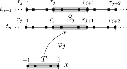
Considering now test functions with support contained within a given element, $S_{j}$, say

$$\phi(r)=l_{i}\big{(}\varphi_{j}^{-1}(r)\big{)}\,\chi_{[r_{j},r_{j+1}]}(r)$$ (38)

where $l_{i}\big{(}\varphi_{j}^{-1}(r)\big{)}$ is the Lagrange polynomial or order $i$ evaluated at the position $x=\varphi_{j}^{-1}(r)$ of the reference element which is mapped into $r$, while $\chi_{[r_{j},r_{j+1}]}$ is the indicator function and thus equal to one in the interval $[r_{j},r_{j+1}]$ and zero elsewhere. Expanding $\boldsymbol{F}^{t}$ over the Lagrange basis of $S_{j}$

$$\big{[}\boldsymbol{F}^{t}\circ\varphi_{j}\big{]}(x)=\sum_{k=0}^{D}\boldsymbol{F}^{t}_{jk}l_{k}(x)\,,$$ (39)

we obtain a set of coupled ordinary differential equations for the coefficients $\boldsymbol{F}^{t}_{ji}$

$$\begin{split}r_{ji}^{2}\partial_{t}\boldsymbol{F}^{t}_{ji}=\big{(}&r^{2}X\boldsymbol{F}^{r},\partial_{r}l_{i}\big{)}_{j,D}\\ &-\frac{1}{w_{i}|\varphi_{j}^{\prime}|}\Big{[}r^{2}\,X\,\boldsymbol{\mathcal{F}}^{r}l_{i}\Big{]}_{r_{j}}^{r_{j+1}}+r_{ji}^{2}\boldsymbol{s}_{ji}\,,\end{split}$$ (40)

where $r_{ji}=\varphi_{j}(x_{i})$ and we used the fact that $(l_{i},l_{k})_{j,D}=\delta_{ik}$. An explicit example of (40) for the continuity equation is given in the Appendix B. Hereafter we will consider only affine maps $\varphi_{j}$, so that the transformation between the reference element $T$ and the finite element $S$ is given by

$$\varphi_{j}(x)=\left(\frac{x+1}{2}\right)r_{j+1}-\left(\frac{x-1}{2}\right)r_{j}\,,$$ (41)

and $|\varphi_{j}^{\prime}|=|r_{j+1}-r_{j}|/2$.

Figure 1 offers a schematic representation of the spacetime grid structure in EDGES. The $D+1$ collocation nodes (i.e. the four filled squares for a polynomial of degree three) are generated and stored on the reference element, $T$, and then mapped onto the finite element $S_{j}$ with an affine transformation, $\varphi_{j}$. Each point on the boundary of an element is associated with two distinct degrees of freedom, so that the corresponding values of the functions can be different there.

This system of equations is coupled with the equations for the evolution of the metric quantities, described in Sect. III.2, and closed with an EOS. In particular we use an ideal-fluid (or $\Gamma$-law) EOS

$$p=(\Gamma-1)\,\rho\,\varepsilon\,.$$ (42)

Expression (40) is clearly a collocation scheme for $\mathcal{D},S$ and $\tau$ on the grid illustrated in Fig. 1, since we can interpret the expansion coefficients as collocated values, i.e. $f_{ji}=f(r_{ji})$ for any function $f$. In our code we evaluate the fluxes, $\boldsymbol{\mathcal{F}}^{r}$, using the relativistic HLLE approximate Riemann solver and evolve numerically the resulting set of equations using a second-order strongly stability preserving (SSP) Runge-Kutta method Gottlieb et al. (2009). We note that, as expected, if $D=0$, then $l_{j}={\rm const.}$, the first term on the right-hand side vanishes and we are left with a standard FV scheme.

A final note concerns the CFL condition needed to ensure the linear stability of the scheme. The linear stability of Legendre pseudospectral methods for hyperbolic equations has been studied in Gottlieb and Tadmor (1991), where it has been shown that $L^{2}$-stability can be obtained if $\Delta t\sim D^{-2}$. As a result, in our code, we use a timestep given by

$$\Delta t=\frac{C_{\text{CFL}}}{(D+1)^{2}}\,\Delta x\,,$$ (43)

where $\Delta x$ is the size of the smallest element, the $C_{\text{CFL}}$ is a coefficient that is reminiscent (but distinct from) the traditional “CFL factor” and has to be determined empirically. This coefficient is usually taken to be $C_{\text{CFL}}\sim 0.2-0.3$, but our numerical experience (at least in 1D) seems to suggest that this condition is overly restrictive as stable evolutions can be obtained with $C_{\text{CFL}}\sim 1$ in most situations.

III.2 Coupling with the spacetime

As discussed in Sect. II.4, in spherical symmetry and with the gauge chosen, the Einstein equations are simple constraints on each spatial slice and thus ODEs in the form

$$\partial_{r}u(t,r)=f(t,r)\,,$$ (44)

which could be easily integrated to very high accuracy. However, instead of using a standard Runge-Kutta method for their integration, we found that a more efficient and accurate approach to solve equations (25) and (26) consists in using an implicit discontinuous spectral ODE solver which makes use of the same grid as the hydrodynamical variables. Such approach has the advantage of obtaining a numerical solution with a degree of accuracy which is of the same order or higher with respect to the one attained for the hydrodynamical variables, without requiring a very small step, as would have been the case for a Runge-Kutta method.

In order to implement this approach it is necessary to allow the solution to be discontinuous across the elements, while imposing the continuity using an interior penalty technique Arnold (1982); Arnold et al. (2002). In particular the discontinuous Galerkin formulation that we use reads

$$\sum_{j=1}^{N}\Bigg{[}\int_{r_{j}}^{r_{j+1}}\partial_{r}u\,\phi\,\mathrm{d}r-\mu_{j}\llbracket u\rrbracket_{j}\,\phi_{j}\Bigg{]}=\sum_{j=1}^{N}\int_{r_{j}}^{r_{j+1}}f\,\phi\,\mathrm{d}r\,,$$ (45)

where $\phi_{j}\equiv\phi(r_{j}^{+})$, $\llbracket u\rrbracket_{j}\equiv u(t,r_{j}^{-})-u(t,r_{j}^{+})$ is the jump term, and $\mu_{j}\sim 1/\Delta r_{j}$ is the penalization coefficient. It is straightforward to see that this penalization term, which we refer to as “upwind penalization” in contrast to the usual symmetric penalization term $\sum_{j=1}^{N}\mu_{j}\llbracket u\rrbracket_{j}\llbracket\phi\rrbracket_{j}$, has the effect of enforcing $u(t,r_{j}^{+})=u(t,r_{j}^{-})$ without affecting the equation for the collocation value in $r_{j}^{-}$.

As customary in the context of DG-SEM-NI methods, we approximate $(\ref{eq:dg.ode})$ as

$$(\partial_{r}u,\phi)_{D}-\sum_{j=1}^{N}\mu_{j}\llbracket u\rrbracket_{j}\,\phi_{j}=(f,\phi)_{D}\,,$$ (46)

so that if we arrange the values of $u(t,r)$ and $f(t,r)$ on the collocation points in two arrays $\boldsymbol{u}(t)$ and $\boldsymbol{f}(t)$, the previous can be written as

$$\boldsymbol{A}\,\boldsymbol{u}(t)=\boldsymbol{f}(t)\,,$$ (47)

where $\boldsymbol{A}$ is a large-sparse matrix. As $\boldsymbol{A}$ does not depend on $t$, in EDGES this matrix is pre-computed, stored and pre-factorized using UMFPACK (see e.g.  Saad (1996)). At each step, then, we have simply to compute $\boldsymbol{f}(t)$ and use the factorized version of $\boldsymbol{A}$ to efficiently compute $\boldsymbol{u}(t)=\boldsymbol{A}^{-1}\boldsymbol{f}(t)$.

III.3 Limiters, spectral viscosity and spectral filtering

It is well known that high-order numerical methods suffer from numerical oscillations in the presence of discontinuities (Gibbs phenomenon). If these oscillations are not suitably handled, they tend to grow out of control and destabilize the method. To overcome this difficulty several different “flattening techniques” have been developed in the context of FD, FV and spectral methods to artificially lower the order of the methods in the presence of shock waves. Some examples are artificial viscosity, flux limiting, PPM or ENO/WENO reconstruction. Many of these techniques are implemented in EDGES and can be activated during the evolution.

III.3.1 Complications of spherical symmetry

While discontinuous Galerkin methods can in general be used in combination with the large majority of flattening techniques, this is not the case in spherical symmetry. The reason for this is that if we consider a function $u$ and interpret any of the flatting methods above as the application of an operator $\mathcal{L}$ to $u$, it can be shown that, for the above mentioned flattening techniques,

$$\int_{\Omega_{j}}u\,\mathrm{d}x=\int_{\Omega_{j}}\mathcal{L}(u)\,\mathrm{d}x\,,$$ (48)

which is the desired behaviour for a conservative scheme in 1D. However, in the case of spherical symmetry, the conservation property that we should satisfy reads

$$\int_{\Omega_{j}}u\,r^{2}\,\mathrm{d}r=\int_{\Omega_{j}}\mathcal{L}(u)\,r^{2}\,\mathrm{d}r\,.$$ (49)

Unfortunately, the property (49) does not hold for almost all of the stabilization techniques which will be discussed in Sect. III.3.2 and which are generally coordinate dependent (the only exception being given by the spectral viscosity method which is inherently a differential operator). In the case of FV codes this is not a problem because the reconstruction is only used in the computation of the fluxes and the volume averages are evolved using the correct cell volume, but in a scheme that works with the actual point-wise value of the solution, this leads to unacceptable variations of the volume integral of $u$ (e.g. of the total “mass”) in the elements with $r\ll 1$ and $r\gg 1$, which in turn leads to the development of large numerical errors and/or instabilities. For this reason it is necessary to introduce a correction to the flattening procedure in the spherically symmetric case.

A naive way to obtain the wanted result would be to modify the operator $\mathcal{L}$ as

$$\tilde{\mathcal{L}}(u)=\frac{1}{r^{2}}\mathcal{L}(ur^{2})\,,$$ (50)

so that $\tilde{\mathcal{L}}$ now satisfies (49). In practice, however, this strategy results, as can be easily foreseen, in large numerical errors near $r=0$ and is this of little use. For this reason we had to adopt a more radical approach and add a “correction step” after the application of $\mathcal{L}$ to enforce (49). In particular we implemented three different strategies which we discuss below.

The first one, which we refer to as “dummy” correction, consists in simply adding to $\mathcal{L}(u)$ a function $C$, constant on every element, such that (49) is satisfied. This is a very simple approach and has the advantage of not increasing the total variation of $\mathcal{L}(u)$ inside the single elements, as conservation is basically obtained at the expense of the amplification of the jumps of $\mathcal{L}(u)$ across the elements. In this way the additional total variation generated by the corrective procedure is concentrated over the grid points which constitute the “finite volume part” of the method.

The second one, which we refer to as “bubble” correction, consists in adding to $\mathcal{L}(u)$ a function $b$, which is a bubble function over each element, i.e. a function which is zero at the edges of the element, such as

$$\big{[}b\circ\varphi_{j}\big{]}(x)=K_{j}(1-x^{2})\,,$$ (51)

where the $K_{j}$’s are chosen in each element so that (49) is satisfied. This approach has the advantage of avoiding the creation of artificial discontinuities at the boundary of the elements, at the price of a small increase in the total variation of $\mathcal{L}(u)$.

Finally the third one, which we refer to “intrinsic” correction, consists in modifying the action of $\mathcal{L}$ so that $L_{q}=\mathcal{L}(L_{q})$ for $q\leq 2$. In this way both (48) and (49) are satisfied. In practice this is obtained by overwriting the low-order coefficients of the discrete Legendre transform (DLT) of $\mathcal{L}(u)$ with the ones of $u$. This method has the advantage of not introducing any unwanted extra total variation and, for this reason, is the one that has the best mathematical properties. The only limitation is that it effectively weakens $\mathcal{L}$ and could thus fail to completely removing the Gibbs oscillations.

All these three techniques can be basically used in combination with any of the stabilization methods which are described in the following Section.

III.3.2 Stabilization techniques

The most commonly used stabilization technique in discontinuous Galerkin methods is based on slope limiting. These methods were originally developed for FV schemes Leveque (1992), but are easily modified to work with discontinuous Galerkin schemes as done by Cockburn and Shu Cockburn and Shu (2001), who introduced the “$\Lambda\Pi_{1}$” limiter based on a generalized version of the “minmod limiter”. In our code we implemented a refined version of this limiter originally proposed by Biswas et al. (1994) and subsequently improved and extended by Krivodonova (2007). This essentially works by recursively limiting the coefficients of the spectral representation of the solution on the various elements. The main advantage of this technique is that it does not require tuning and it is usually very reliable, while its main limitation is that its use often results in excessive flattening of the solution in the presence of discontinuities. Moreover we found that all these methods perform rather poorly in conjunction with the correction techniques outlined above and for this reason we have rarely used them.

Another method implemented in EDGES is the “spectral viscosity” method first proposed by Maday et al. Maday et al. (1993) in the context of Legendre pseudospectral methods for conservation laws. This method consists in the addiction to the right hand side of (40) of a term

$$-\varepsilon_{D}\,(Q\,\partial_{x}\boldsymbol{F}^{t},\partial_{x}\phi)_{D}\,,$$ (52)

where $\varepsilon_{D}$ is a coefficient depending on the number of grid points and $Q$ is a viscosity kernel whose action on a scalar function $u$ reads, in every element,

$$\big{[}Qu\big{]}(x)=\sum_{k=0}^{D}\hat{Q}_{k}\hat{u}_{k}L_{k}(x)\,.$$ (53)

Here, $\hat{u}_{k}$ are the coefficients of the DLT of $u$ and $\hat{Q}_{k}$ are real numbers such that

$$\hat{Q}_{k}=0\,, \textrm{for}\quad k\leq m_{D}\,,$$ (54a)

$$1-\bigg{(}\frac{m_{D}}{k}\bigg{)}^{4}\leq\hat{Q}_{k}\leq 1\,, \textrm{for}\quad k>m_{D}\,.$$ (54b)

Note that $m_{D}$ effectively plays the role of the cut-off frequency of the filter. Meday et al. Maday et al. (1993), were able to show that, in the context of scalar conservation laws in 1D and using only one domain, this method is able to stabilize the scheme, without spoiling its spectral accuracy if

$$\varepsilon_{D}\sim D^{-\theta}\,,\quad\textrm{for}\quad D\gg 1\,,$$ (55)

where $theta$ is just an exponent such that $0<\theta\leq 1$ and

$$m_{D}\sim D^{q/4}\,,\quad\textrm{for}\quad 0<q<\theta\leq 1\,.$$ (56)

In our code we have set

$$\varepsilon_{D}=\mu\frac{\Delta t}{N}\frac{1}{D}$$ (57)

and

$$\hat{Q}_{k}=f\,, \textrm{for}\quad k\leq m_{D}\,,$$ (58a)

$$\hat{Q}_{k}=f+1-\bigg{(}\frac{m_{D}}{k}\bigg{)}^{4}\,, \textrm{for}\quad k>m_{D}\,,$$ (58b)

where $\mu$, $f$ and $m_{D}$ are set by the user (standard reference values are $\mu=1,f=0$ and $m_{D}=0,1$).

Besides being particularly dissipative, this method has the important advantage that it can be adapted to spherical symmetry by modifying (52) as

$$-\varepsilon_{D}\,(r^{2}\,Q\,\partial_{r}\boldsymbol{F}^{t},\partial_{r}\phi)_{D}\,.$$ (59)

In this way, the condition (49) is satisfied without the need of adding corrective terms. In EDGES, the term (59) is added using an operator-splitting technique, so that its use corresponds to the application of a linear filter. This is discretized with two different techniques: locally on each element, or globally, using an interior penalty technique. We call the latter approach “interior-penalty spectral-viscosity” (IPSV) stabilization. While the first approach is completely local, the second one is able to relax also the jump terms between the elements. The main drawback of this method, however, is that we have found that the quality of the results can be quite sensitive to the tuning of $\mu$ and $m_{D}$, which are necessarily problem dependent.

The third method implemented in EDGES is usually referred to as “spectral filtering” (see e.g.  Canuto et al. (1988)). The idea behind this technique is to filter the numerical solution, or its time derivatives, with a low-pass filter in order to remove high-frequency components and keep the Gibbs oscillations under control. In the context of Legendre pseudospectral methods, this filtering, which we indicate with $\mathcal{F}_{D}$, reads

$$\big{[}\mathcal{F}_{D}u\big{]}(x)=\sum_{k=0}^{D}\sigma\bigg{(}\frac{k}{D}\bigg{)}\,\hat{u}_{k}\,L_{k}(x)\,,$$ (60)

where $\hat{u}_{k}$ are the coefficients of the Legendre expansion of $u$ and $\sigma(\eta)$ is a filter function of order $p$ in the Vandeven’s sense, that is a function $\sigma\in C^{p}\big{(}\mathbb{R}^{+};[0,1]\big{)}$ such that

$$\cdot\leavevmode\nobreak\ \sigma(0)=1\,;$$ (61)

$$\cdot\leavevmode\nobreak\ \sigma^{(k)}(0)=0\,, k=1,2,\ldots,p-1\,;$$ for (62)

$$\cdot\leavevmode\nobreak\ \sigma(\eta)=0\,, \eta\geq 1\,;$$ for (63)

$$\cdot\leavevmode\nobreak\ \sigma^{(k)}(1)=0\,, k=1,2,\ldots,p-1\,;$$ for (64)

where $f^{(p)}(x)$ denotes the $p$-th derivative of $f$ in $x$. These schemes were studied by Hesthaven and Kirby Hesthaven and Kirby (2008), who showed that if $\sigma(\cdot)$ is a filter of order $p$, and $u\in C^{p}(-1,1)$, then

$$\big{|}u(x)-\mathcal{F}_{D}u(x)\big{|}\leq D^{1-p}\|u^{(p)}\|_{L^{2}(-1,1)}\,,$$ (65)

so that, if $p\sim D$, the filter does not spoil the spectral accuracy of the method.

The effects of filtering on the stability of the numerical method can be intuitively understood from the fact that some filters, in particular the exponential filter of order $p$,

$$\sigma(\eta)=\exp\Big{[}-\mu(D+1)\frac{\Delta t}{\Delta x}\eta^{p}\Big{]}\,,$$ (66)

can be interpreted as equivalent to the use of numerical diffusion of order $p$ and strength $\mu$ Meister et al. (2009). At present, however, a mathematical understanding of the impact of filtering on the accuracy and the stability of Legendre pseudospectral methods is still lacking Hesthaven and Kirby (2008).

EDGES provides a number of different filter functions, but the most used are the exponential filter (66), which is only an approximate filter, but which is very popular due to its flexibility Canuto et al. (1988), and the “Erfc-Log filter” proposed by Boyd Boyd (1996),

$$\sigma(\eta)=\frac{1}{2}\mathrm{erfc}\Bigg{\{}2p^{1/2}\bigg{(}|\eta|-\frac{1}{2}\bigg{)}\sqrt{\frac{-\log[1-4(\eta-1/2)^{2}]}{4(\eta-1/2)^{2}}}\Bigg{\}}\,,$$ (67)

which is a semi-analytic approximation of the Vandeven’s filter,

$$\sigma(\eta)=1-\frac{\Gamma(2p)}{\Gamma(p)^{2}}\int_{0}^{\eta}\big{[}t(1-t)\big{]}^{p-1}\mathrm{d}t\,,$$ (68)

where $\Gamma$ is the Euler Gamma function. Note that it is customary to use filters of order $p\sim 2D$ or larger when expecting regular solutions and $2D+1$ is a reasonable value for a strong filter such as Erfc-Log.

The main limitation of spectral filtering is that, being a high-order linear method, it cannot completely remove the Gibbs oscillations. This is a consequence of the well-known Godunov theorem stating that no linear monotonicity-preserving method exists of second-order or higher (see e.g.  Leveque (1992)). The idea is, instead, to allow for small oscillations of the numerical solution at the location of shocks, while preventing them from growing out of control. In our numerical experience we found that spectral filtering is a robust and viable alternative to slope limiting in the shock-tube case, where its use often results in a sharper resolution of the discontinuities, and, at the same time, it is well-behaved in the spherically symmetric case. Spectral filtering seems also to be much less sensitive than the spectral viscosity methods to the tuning of the parameters of the filter functions. Finally, we point out that, in contrast to IPSV and slope limiters, this technique is completely local in the sense that its application in a given element does not require the knowledge of the solution elsewhere. For these reasons, most of the results that we will show in the next Sections were obtained with the use of spectral filtering.

Figure 2: Solution for the rest-mass density of a relativistic shock tube with different stabilization techniques. The solid black line represents the exact, analytic solution, while the red crosses and the blue squares refer to the use of the two different DLT filters, i.e. the Erfc-Log and the exponential filter, respectively. The blue triangles and the violet circles refer instead to the use of the IPSV filter and of high-order slope limiters, respectively. To avoid excessive cluttering, only a data point every five is shown. The results were obtained on a grid of $N=200$ elements with a polynomial of degree $D=3$.

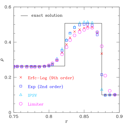
Before doing that, however, and to illustrate the difference between the various stabilization techniques, we show in Fig. 2 a comparison of the results obtained using different filters, while keeping all the other discretization parameters fixed. In particular, we show the results obtained in the case of a relativistic shock tube in flat spacetime. The details of the physical setup will be given in Sect. IV.1, here instead we focus on the effects of the different stabilization techniques. As anticipated we find that slope-limiting, even in their high-order variant, result in a much larger smearing of the shock front, then all the other methods. The 9th order Erfc-Log filter yields a much sharper resolution of the shock and a stable evolution, even tough, as discussed before, filtering does not have such a strong mathematical basis, while slope-limiting is known to yield a total-variation diminishing in mean (TVDM) scheme Cockburn and Shu (2001). The best overall results are the ones obtained with the second-order exponential filter, for which we used a small strength factor, $\mu=1$, and the IPSV technique with $\mu=1$ and $\hat{Q}_{k}=1$. We remark that the results obtained with these last two methods are very similar since, as discussed before, the action of an exponential filter is roughly equivalent to that of a spectral viscosity. The results in Fig. 2 obtained on a grid of $N=200$ elements with a polynomial of degree $D=3$.

III.4 Treatment of low-density regions

The treatment of interfaces between vacuum region and fluid regions is one of the most challenging problems in Eulerian (relativistic) hydrodynamics codes (see e.g.  Galeazzi (2008); Kastaun (2006); Millmore and Hawke (2010)). The most commonly used approach to treat vacuum regions is to fill them with a low-density fluid, such that if a fluid element is evolved to have a rest-mass density below a certain threshold, it is set to have a floor value and zero coordinate velocity Font et al. (2002); Baiotti et al. (2005). This approach works reasonably well and has been adopted by the vast majority of the relativistic-hydrodynamics codes. Nevertheless, the introduction of this “atmosphere” creates several numerical difficulties. First of all, this approach is gauge dependent and, for example, a star can accrete or lose mass from/to the atmosphere due to oscillations in the coordinate variables. Secondly, this approach often results in the introduction of errors at the surface of the star, which, on the one hand, usually have small influence on the overall dynamics because of the small momenta involved, but which, on the other hand are relatively large if compared with the magnitude of the involved quantities at the surface. Finally, and most importantly, it is possible that the algorithm governing the evolution of the floor can couple with the Gibbs oscillations, leading quickly to their amplification and destabilizing the scheme (After-all, the introduction of an atmosphere treatment is de-facto equivalent to the use of a boundary condition and this can very well lead to an unstable algorithm). For this reason this procedure could not be used in a straightforward way in our code, but required a particular care.

Other solutions, such as the use of the equations in Lagrangian form, e.g.  Gabler et al. (2009), the use of moving grids techniques e.g.  Gourgoulhon (1991), or the use of suitable limiters at the surface Galeazzi (2008), do not suffer from these issues, but are restricted to the spherically symmetric case. As our code is meant to be a prototype code to study the viability of DG methods for relativistic hydrodynamics, the use of these techniques would have defeated our purpose.

As a result, several different approaches were implemented and tested in EDGES to overcome the difficulties with the atmosphere discussed above. The main idea behind all these approaches was to use stronger stabilization techniques at the interfaces between fluid and vacuum regions. Unfortunately all these techniques performed quite poorly because they resulted in an unacceptable lowering of the resolution at the surface and thus in large numerical errors. Moreover, in the spherically symmetric case, the situation is greatly worsened by the fact that these errors tend to build up coherently while traveling towards the center. For example, in the case of a neutron star, they tend to be amplified by a factor $R/r\sim 10^{3}$, $R\sim 10$ being the radius of the star and $r\sim 0.01$ being the location of the closest grid point to the center.

Figure 3: Division of an element into control volumes for the spectral-volume method applied at the fluid-vacuum interface. The values of the solution $u$ on the collocation points (filled squares) are interpreted as volume-averaged values of the solution in appropriate control volumes (hollow diamonds denote the boundaries). These values are then used to generate a reconstructed solution $\mathcal{R}u$ using an adapted slope-limiter method.

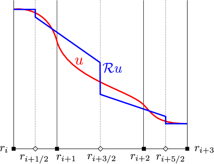
Within EDGES a solution to this problem was eventually found with the use of a method that is, at the same time, oscillation-free and capable of obtaining high-enough resolution at the surface. In particular, we derived a “sub-element method” approach that we later discovered to be very similar to the spectral volumes (SV) method already suggested by Wang Wang (2002). In this method, we first flag those elements in which the rest mass density falls below a certain threshold. Secondly we interpret the value of the solution on the collocation points of those elements as being the volume-averaged value of the solution on appropriated control volumes. Finally these values are evolved as in a FV scheme: a linear reconstruction with slope limiting is used to compute the value of the primitive variables at the interface of the control volumes and the HLLE approximate Riemann solver is used to compute the fluxes.

The structure of the grid used for this spectral volume method is shown in Fig. 3. The control volumes are simply obtained by considering the points of the dual mesh as the cell interfaces, while their volume has to be corrected to take into account the weights of the Gaussian quadrature associated with the primal grid. The linear reconstruction can be performed only for the interior control volumes, while for the control volumes at the boundary of each element we already have the value of the solution at one side of the control volume, thus we are forced to reconstruct the solution there as a constant. In our tests we found that the “superbee” Font (2008) limiter is the one which guarantees the best results among the ones that we tested. For this reason, all the results shown in the following make use of this limiter.

Figure 4: First shock-tube test. Shown with solid lines are the exact solution for the rest-mass density (black line), the velocity (blue line), and the specific internal energy (red line). The corresponding numerical solution is represented by the black crosses, the blue triangles, and the red squares, respectively. To avoid excessive cluttering we show only one point every $15$ of the numerical solution. The results were obtained on a grid of $N=500$ elements with a polynomial of degree $D=3$.

The important advantage of this approach, with respect to a more traditional approach in which the troublesome elements are split into equal-size cells and a classical FV method is used, see e.g.  Touil et al. (2007), is that no interpolation is required in the switching from/to the discontinuous Galerkin method. The coupling between the two methods is also very natural and is done through the Riemann solvers between the elements. Again no special treatment is required to handle different type of elements: the DG ones and the SV ones. The main limitation of this approach is that, as we do not increase the number of degrees of freedom in the flagged elements, it has the effect of reducing the accuracy to second order where it is used. As it will be shown in Sect. IV.4, this seems not to be limiting the accuracy of our code, probably because the use of the SV method is confined to small regions containing low-density fluid. In the case of a neutron star, for example, the use of the SV method is typically limited to one element containing the surface of the star.

As a final remark we note that, as we are working with a nonuniform grid, the slope limiting method in its standard form, also used by us, is not guaranteed to be TVD and/or second order Berger et al. (2005). Again this seems not to be a problem in practice.

IV Numerical tests

In what follows we present the results obtained from some of the tests performed with EDGES. These tests have been chosen because they highlight the capabilities of our code in idealized settings, such as in the simulation of shock tubes and shock waves, and in more “astrophysically motivated” settings, such as in the simulation of the dynamics of spherical stars and of the gravitational collapse to black hole. In all cases considered, the evolution has been made employing an ideal-fluid EOS to take into account for non-isentropic transformations, such as shock-heating effects.

IV.1 Shock tubes

The first tests performed are shock-tube tests and, more specifically, we first present the results obtained in the case of two standard benchmarks for relativistic-hydrodynamics codes described in Martí and Müller (2003). These are referred to as “blast-wave” problems $1$ and $2$ in Martí and Müller (2003), and are essentially one-dimensional flat-space Riemann problems.

Figure 5: Rest-mass density profile for the second shock-tube test. Shown with different lines are the exact solution (solid black), the solution obtained with the ECHO code Del Zanna et al. (2007) (dotted blue). Both codes use $1000$ cells/elements and algorithms at fifth order; EDGES also uses a exponential filter with $\mu=1,p=2$.

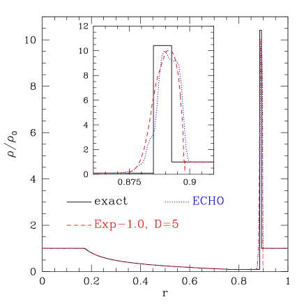
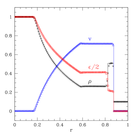
The first problem describes the propagation of a relativistic blast wave through a low-density medium. The solution obtained with EDGES, as well as the analytic solution, are shown in Fig. 4, where the solution is computed using polynomials of degree three (i.e. $D=3$) and $500$ elements (i.e. $N=500$). The stabilization is obtained with the use of an Erfc-Log filter of 9th order, which has been applied directly to the conserved variables in the regions where they fail to be monotone at every timestep. As it can be seen from the figure, the stabilization is strong enough to eliminate any oscillation, thus reducing the order of the method to the expected first-order near the discontinuity, yet with a very small smearing of the shock.

Figure 6: The same as in Fig. 5, but with a magnification of the shock and a comparison of the results at different orders $D$ of the polynomial representation of the solution. Note that the accuracy with which the shock location is founded increases with $D$

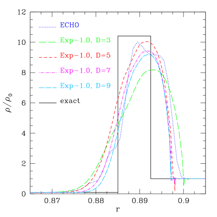
The second shock-tube problem is similar to the first one, but is much more extreme. This benchmark is considered to be a challenging test also for modern HRSC codes Martí and Müller (2003). The main difficulty is to handle the very high compression ratios, typical of relativistic hydrodynamics, produced in this case. In Fig. 5 we show a comparison of the results obtained with our code when using the exponential filter (66) at second-order (i.e. $p=2$) with $\mu=1.0$, which is employed in the same way as the Erfc-Log filter in the previous test. Also shown for a comparison is the solution obtained with the high-order HRSC code ECHO Del Zanna et al. (2007), which was kindly provided by Olindo Zanotti. The ECHO code uses HLLE Riemann solver and monotonicity-preserving reconstruction at fifth order Suresh and Huynh (1997), while for EDGES we employed fifth-order polynomials. Furthermore, the comparison is made when using the same number, $1000$, of cells (for ECHO) and of elements (for EDGES); for both codes, in fact, we expect a convergence order (on smooth solutions) of the type $\Delta x^{-p}$, with $\Delta x$ being the width of each cell/element and $p$ being the order of the scheme. Note, however, that, while in ECHO high order is obtained with the use of data across multiple cells, in EDGES this is attained with the use of a polynomial representation of the solution in each element. Thus the EDGES code actually uses around six times more grid points than the ECHO code. Nevertheless, we argue that this is the correct comparison because, as mentioned before, the convergence properties of the two codes once the reconstruction procedure and the order of the polynomial representation is fixed, scale with the width of the cells/elements. This kind of comparison, where results obtained with discontinuous Galerkin and finite volume methods are obtained using the same number of elements/cells, but different number of degrees of freedom has already been discussed in the literature, see e.g. Zhou et al. (2001).

As can be seen from Fig. 5 the quality of the solution obtained by the two codes is comparable, with the solution obtained by the EDGES code being slightly closer to the exact position of the shock, but also showing signs of Gibbs oscillations ahead of the shock. Overall, the exponential filter can prevent the oscillations from growing and yields the best results when compared to the other flattening techniques discussed above. A more quantitative estimate of the quality of the numerical solution can be obtained by looking at the ratio $\sigma/\sigma_{\mathrm{exact}}$, between the observed compression ratio and the analytic one Martí and Müller (2003). We obtain a value of $0.96$ with both ECHO and EDGES. At lower resolution, i.e. using only $400$ elements, we obtain, for EDGES, a value of $0.60$ which is close to the ones reported for PPM at the same resolution: i.e. $\sigma/\sigma_{\mathrm{exact}}\simeq 0.54-0.69$ Martí and Müller (2003). We conclude therefore that in the case of discontinuous solutions, DG methods behave similarly to FV methods with the same number of elements/regions.

It is worth stressing that while for ECHO the fifth order represents the largest achievable, the EDGES code can perform this very severe test also with higher-order polynomials. This is shown in Fig. 6, where we report again the exact solution shown in Fig. 5 and compare it with the numerical one for $D=3,5,7$ and $D=9$. Of course the mathematical convergence in all of the different solutions is still only at first order, but it is remarkable to see that the code can handle such large shocks even when $D=9$ and that the position of the shock and of the contact discontinuity become increasingly accurate as $D$ is increased. Overall, the solution with $D=5$ is the one yielding the closest match with the density right behind the shock and we have not considered orders higher than this in most of the subsequent tests. As a final remark we note that, to the best of our knowledge, this is the first time that a shock-tube test in relativistic hydrodynamics has been computed using a method of this order.

IV.2 Spherical shock reflection

Figure 7: The same as Fig. 4, but for the spherical shock-reflection test with a Lorentz factor of $W=1000$. To avoid excessive cluttering in the main frame of the picture we plot only a point every five of the numerical solution, while the inset shows the solution on all the collocation points.

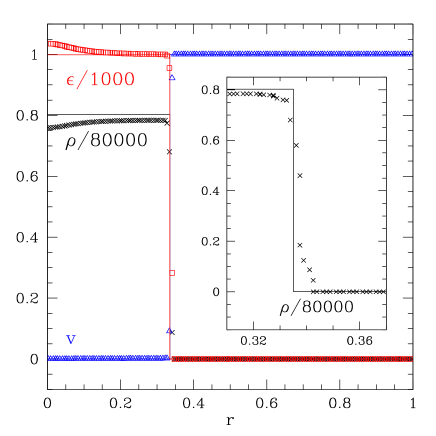
Another classical benchmark for relativistic-hydrodynamics codes is the spherical shock-reflection test. This is the relativistic version of the classical Noh test and its setup is described in detail in Martí and Müller (2003). The initial data consist in a cold fluid converging at the center of the domain. As the fluid flows towards the center, a hot dense shell of matter is formed and a shock wave is propagated outwards. In this situation it is possible to generate arbitrarily high compression ratios by increasing the Lorentz factor of the ingoing flow. This is a peculiarity of relativistic hydrodynamics and, again, the key point of the test is to assess the capability of the numerical methods to handle such strong density contrasts.

This problem is also interesting to assess the quality of the correction procedure for the filtering in spherical symmetry. In particular, the quality of the results depends on the used correction procedure: they are of comparable quality when using the “dummy” and the “bubble correction” procedures (the former being slightly better), while the “intrinsic” correction yields a filtering which is too weak to guarantee stability. This is not a surprise since with the intrinsic procedure we are not able to filter the coefficients of order less than two in the Legendre expansion, so that we cannot reduce the order of the method below the second even with a strong targeted filter.

Figure 8: $L^{2}$-error in the spherical accretion test as a function of the number of elements $N$. Crosses and squares refer to the errors on $C_{1}$ and $C_{2}$, respectively, while the black, blue and red colors denote refer to the simulations using third, fourth, and fifth-order polynomials. Finally the dashed lines show the slopes associated with third, fourth, and fifth-order convergence.

In Fig. 7 we present the results obtained for a flow with $W=1\,000$ solved using polynomials of degree three, on $200$ elements and with an Erfc-Log filter with $p=4$ and a dummy correction. As shown in the figure, the filtering procedure is able to suppress any spurious oscillation and the shock front is captured within two elements, i.e. eight collocation points. The average relative error on the compression level is of $1.4\,\%$, comparable with the $2.2\,\%$ reported by Romero et al. Romero et al. (1996) using FV with a minmod reconstruction on a grid with the same number of cells. Furthermore, as in Romero et al. Romero et al. (1996), the error in $\epsilon$ and $\rho$ increases in the inner part of the solution. This is due to the well known wall-heating effect and is due to the small but nonzero dissipative and dispersive features of the numerical methods (see Noh (1987); Rider (2000) for an extended discussion of this effect).

IV.3 Spherical accretion onto a Schwarzschild black hole

Having verified the capability of our code to handle shock waves, we next present some results concerning its accuracy in the case of regular solutions. In particular, we consider the case of spherical accretion onto a Schwarzschild black hole in the Cowling approximation (i.e. with a fixed spacetime). An analytic solution exists in the case of stationary flows and was first presented by Michel Michel (1972) and later used as a numerical test for other numerical codes, for example by Romero et al. (1996). This solution can be described in term of two constants:

$$C_{1}\equiv\sqrt{-g}\,J^{r}\,,$$ (69)

and

$$C_{2}\equiv\sqrt{-g}\,T^{r}_{\phantom{r}t}\,.$$ (70)

Figure 9: The same as in Fig. 8, but when the error is shown as a function of the polynomial degree when the number of elements $N$ is kept fixed (black for $N=20$ and red for $N=30$). Note that an exponential convergence is measured.

In our simulation we consider a spherical shell with extent $3-N/40\leq r\leq 20$ in the spacetime metric of a Schwarzschild black hole of unit mass, while the initial conditions for the hydrodynamical variables describe a low-density fluid at rest with respect to an observer at infinity. At $t=0$ we start injecting higher-density fluid from the outer boundary and after a short transient the solution reaches stationarity, allowing us to measure $C_{1}$ and $C_{2}$ and to compare them with the analytic values fixed by the outer boundary condition.

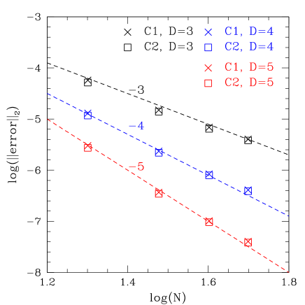
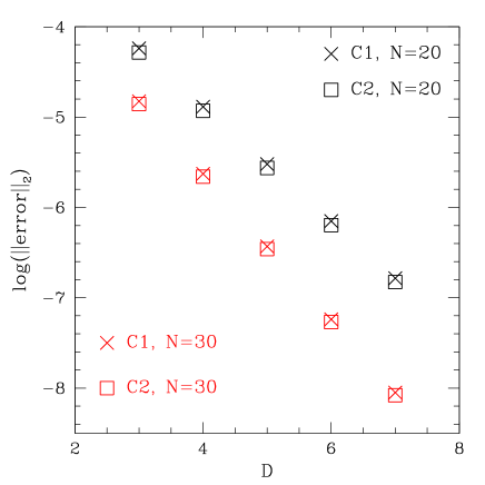
In Fig. 8 we show the $L^{2}$-norm of the error for $C_{1}$ and $C_{2}$ as a function of the number of elements $N$, and for different orders $D$ of the polynomials used for the representation of the numerical solution over the single elements. The stabilization was obtained using an exponential DLT filter of order $2D$ and strength $\mu=1.0$, corrected using the “dummy” strategy. Clearly, the errors computed from $C_{1}$ and from $C_{2}$ are basically identical. More importantly the convergence order is the one that one would expect from the theory: third, fourth, and fifth-order using third, fourth, and fifth-order polynomials, respectively.

A complementary measure of the convergence properties of the code is shown in Fig. 9, where we report the $L^{2}$-norm of the error obtained after keeping fixed the number of elements, $N=20,30$, but changing the order of the polynomials used for the representation of the solution. As expected, SDGM schemes behave in this case as multi-domain spectral methods Canuto et al. (2008), with the error decreasing exponentially with the polynomial degree. This is indeed what we observe in Fig. 9, where the errors decrease exponentially by almost three orders of magnitude for both $C_{1}$ and $C_{2}$, and at both resolutions. No sign of saturation appears in the error and we find it remarkable that the same method that was able to capture so sharply the discontinuous solutions in the previous tests, is also able to attain exponential convergence in smooth flows.

IV.4 Linear oscillations of spherical stars

The results presented so far refer to situations that are somehow idealized and are meant mainly as a way to highlight the code’s properties with respect to shock capturing, filtering correction and accuracy on smooth solutions. We next present the results obtained in tests describing systems of more direct physical interest. Furthermore, in contrast to the previous tests, the matter will not be considered as a test-fluid and the spacetime will be properly evolved.

A first interesting test is the study of linear oscillations of spherical stars. The initial data considered describes the equilibrium configuration of a self-gravitating fluid sphere, described by a polytropic equation of state, $p=K\rho^{\Gamma}$, and is obtained by integrating the Tolman-Oppenheimer-Volkoff (TOV) equations, as described by Tooper (1965), and interpolating the result on the computational grid used by EDGES. The system is then evolved under the sole effects of numerical perturbations, mainly due to the interpolation errors in the generation of the initial data and to the interaction between the star and the atmosphere. Note that in order to avoid the presence of collocation points at $r=0$, we stagger our numerical grid so that the $r=0$ point falls at the centre of the first element and we use only polynomials of odd degree.

Figure 10: Evolution of the central rest-mass density normalized to its initial value for a stable TOV and evolved with a polynomial of degree five. Different lines refer to different resolutions: solid black, dashed blue and dotted red for $N=75\,,100$ and $125$, respectively. Shown in the insets are the evolution at the initial time (i.e. $t\lesssim 2$ ms) and when the error at the surface is released triggering new small-scale oscillations (i.e. $t\sim 45$ ms).

More specifically, we have considered a TOV constructed with a polytropic EOS having $K=100$ and $\Gamma=2$ and whose initial central density is $\rho_{c}=1.28\times 10^{-3}$. This could be taken to represent a stable, nonrotating, neutron star with gravitational mass $M=1.4\,M_{\odot}$ and areal radius $R=9.6\,M_{\odot}\simeq 14.2$ km. The degree of the polynomial basis is five and an Erfc-Log filter of order eleven is used to ensure a stable evolution. This filter is corrected with the “intrinsic” procedure outlined in Sect. III.3.1 and is applied to the right-hand-side of the time stepping scheme. This results in a very weak stabilization algorithm whose main effect is to diffuse back into the atmosphere the numerical errors that would otherwise accumulate at the surface of the star and destabilize high-resolution runs. The latter, in fact, have very low intrinsic viscosity and run for many more timesteps on timescales of $100$ ms or longer (we recall that the dynamical timescale for this star is of the order of $0.7$ ms).

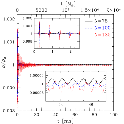
In Fig. 10 we show the evolution of the central density for three of these runs using different resolutions. They span a time frame of $20\,000\,M_{\odot}\sim 100\ \mathrm{ms}$, with the grid extending over the range $0\leq r\leq 15$ and being composed by $N=50,75,100,125$ and $150$ elements.

Figure 11: Power spectral density computed from the first $5000\,M_{\odot}$ of the evolution of the central rest-mass density shown in Fig. 10. Different line types and colors refer to the different resolutions used (see legend). Shown as vertical dotted lines are the eigenfrequencies computed from linear perturbation theory.

The dynamics is similar among the three runs, with the central density first exhibiting a “burst” with a variation of the order of $0.12\,\%$, which is due to the fact that the star is “cut” by our interpolation algorithm of the initial data there where the density falls below the atmosphere threshold. This phase is magnified by the inset in the top of the figure. In a second stage the “burst” is quickly damped and the star starts to vibrate radially with its characteristic eigenfrequencies and eigenmodes under the effects of numerical perturbations, mainly at the surface of the star. In a third phase these oscillations are damped by the numerical viscosity, which depends on the resolution, and by the crude treatment used to represent the surface of the star. High-frequency modes are damped quickly while low-frequency modes have longer damping times. As a result, towards the end of the simulation we are left only with slowly-damped sinusoidal oscillations associated with the $F$-mode. This is particularly evident in the $N=75$ run, which has the largest numerical viscosity.

The evolution is stable for all the resolutions that we have considered, but a careful examination of the behaviour of the central density reveals the existence of a fourth stage of the dynamics in some of the runs with lower resolution. More specifically, it is possible to note that during the third phase of the dynamics numerical errors accumulate at the surface of the star, producing small variations in the density profile near the atmosphere. When these variations are large enough so that they cannot be controlled by the employed flattening methods, they are “released” and new energy is pumped into the high-frequency modes, starting a new phase in the dynamics. This happens at around $45$ ms for the $N=75$ run in Fig. 10, when a small high frequency component modulated by the $F$-mode suddenly appears, as shown by the inset at the bottom of the figure. The same happens around $80$ ms for the $N=100$ run, while this phenomenon is not observed within the simulation time for higher resolution runs. Although the onset of this “energy release” at the surface can be delayed with the use of stronger filtering, it occurs only on a secular timescale and it does not affect the stability of the star. As a result, the central density keeps oscillating with a very small amplitude, of the order of $10^{-3}\,\%$, even if, as discussed in Sect. III.3.2, perturbations at the surface tend to be greatly amplified when they reach the center as an artifact of the spherical symmetry. For this reason we believe that the energy release does not impact the quality of our simulations.

Figure 12: Absolute relative difference between the estimated eigenfrequencies and the ones computed from linear perturbation theory, shown for different modes and as a function of the resolution. The lower-order modes are not considered because their error is smaller than the nominal one of the power spectral density and we report only the values for which a reliable measure of the error was possible. Finally, indicated as black dashed lines are the slopes associated with fifth and sixth-order convergence.

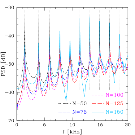
A traditional measure of the accuracy of general-relativistic hydrodynamics codes is the comparison of the power spectrum of the oscillations of TOVs against the values provided by linear perturbation theory. In Fig. 11 we make this comparison by showing the power spectrum of the first $5\,000\,M_{\odot}$ of the evolution of the central density for different resolutions. The vertical dotted lines represent the eigenfrequencies computed from perturbation theory, which were kindly provided us by Kentaro Takami and computed using the method described in Yoshida and Eriguchi (2001). We note that, even at the lowest resolution, EDGES shows a perfect agreement between the observed proper frequencies and the perturbative ones for the $F$-mode and the first four overtones, $H1,H2,H3$ and $H4$. Furthermore, as the resolution increases we are able to match more and more modes to the point that, with the $N=150$ run, we match the first ten modes to a very good precision. We also note that the $N=150$ run gives evidence of some nonlinear features in the spectrum, which shows considerable power also in its high-frequency part.

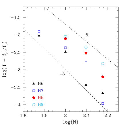
A more quantitative measure of the convergence of the power spectrum is shown in Fig. 12, where we report as a function of the resolution the relative difference between the measured frequencies for the overtones $H6,H7,H8$ and $H9$, and the ones computed from perturbation theory. More specifically, the numerical frequencies were computed from the data during the first $5\,000\,M_{\odot}$ by using the procedure proposed in Agrez (2007). Namely, we computed the discrete Fourier transform (DFT) of the data with an Hanning window and used a three point interpolation of the power spectrum to correct for the incoherency error and determine the correct eigenfrequencies (this procedure is conceptually equivalent to a Lorentzian fit of the peaks of the DFT). Note that the lower-order modes are not shown because their precision is such that the error on those frequencies is well below the nominal uncertainty of the DFT and is basically dominated by the error on our measure. (The values of the error is not shown for those resolutions/frequencies that could not be determined in a reliable way: namely, the $H8$ and $H9$ modes for the $N=75$ run.). Overall, we find that the measured convergence rate depends somehow on the specific mode, but it is compatible with a fifth-order convergence rate (cf. the fifth and sixth-order convergence rates which are shown as dashed lines). As we will comment later on, this results indicates that our largest source of error on the frequencies is not dominated by the low-order FV approach used at the surface of the star. Rather, the behaviour in Fig. 12 shows that in the case of global quantities such as the oscillation frequencies of a TOV, the treatment of the surface is not the most critical element of the “error budget” in EDGES.

Figure 13: Estimated damping rates for various eigenmodes as a function of the resolution as computed by EDGES in 1D and by Whisky in 3D. Black triangles, blue squares and red circles refer respectively to the $F\,,H1$ and $H2$ modes, while filled/hollow points distinguish the estimates with EDGES from those with Whisky. Finally the dashed lines show the estimated convergence order.

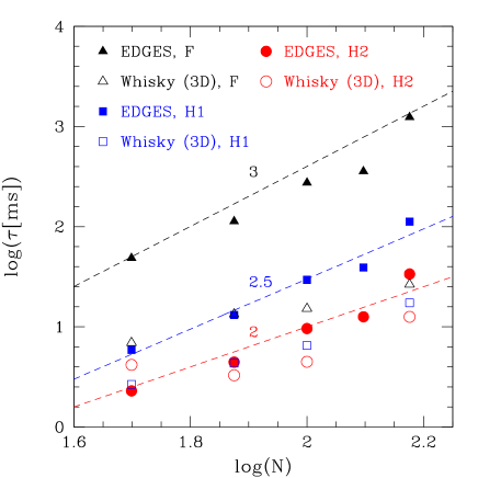
As a concluding consideration we note that in a recent work Cerdá-Durán Cerda-Duran (2009) has proposed to measure the numerical bulk viscosity of general-relativistic hydrodynamical codes by looking at the damping time of the $F$-mode in the case of oscillating TOVs. In particular, the rate of change with resolution of the damping time (and which clearly increases with resolution) can be used as a measure of the convergence rate of the code. To explore this interesting suggestion we have computed the damping time by analysing more systematically the evolution of the central density. More specifically, using a sampling frequency of $\approx 1\,M_{\odot}$, we have built a discrete signal which was then divided into chunks of $512$ points with an overlap of $128$ points. A DFT of each chunk was then computed using an Hanning window and the power of the signal at the frequency associated with each mode was computed with a linear interpolation of the absolute value of the DFT. In this way we obtained an estimate of the energy in the mode for each time window. Finally we performed a least square fit of an exponential function to determine the damping time. (We have estimated the accuracy of this procedure to be better then $10\%$, on the basis of tests performed with signals of known spectral properties.)

In Fig. 13 we show the results of this measure when made on different modes. The data for the $N=50\,,75$ and $N=100$ runs have been obtained by windowing the evolution in the interval $0\leq t\leq 5\,000$ to avoid spurious values due to the fourth phase of the dynamics described above, while for the $N=125\,,150$ runs it was necessary to use the full data in the interval $0\leq t\leq 20\,000\approx 100\ \mathrm{ms}$ to obtain a reliable estimate of the damping time for the $F$-mode. As a comparison, we also report the results obtained in 3D using the Whisky code Baiotti et al. (2005); Giacomazzo and Rezzolla (2007); Pollney et al. (2007); Schnetter et al. (2004), when computed using a similar procedure. The simulations with Whisky were done using a PPM reconstruction and the HLLE Riemann solver for the hydrodynamics and using a fourth-order FD scheme for the evolution of the spacetime on a uniform grid also covering $0\leq r\leq 15$.

We find that the convergence order of the damping time of the $F$-mode with Whisky is one, in agreement with the results reported by Cerda-Duran (2009) for the COCONUT code Dimmelmeier et al. (2002, 2005). In Cerda-Duran (2009) it was argued that the reason why the order reduces to first is that the damping is active mainly at the surface of the star, where the numerical methods are only first order. The results found with EDGES show however a different behaviour, with the order of the damping being $3,2.5$ and $2$ for the $F$, $H1$ and $H2$ modes, respectively. Because the treatment of the surface in EDGES can be seen as a variant of the FV method used by both Whisky and COCONUT and is therefore only first-order accurate, our results suggest that the coefficient of the first-order (and surface-induced) error is much smaller than the coefficient of the error coming from the high-order filtering procedure, which then becomes the dominant source of damping. This is in agreement with the high convergence order found in the measurement of the eigenfrequencies (cf. Fig. 12).

Figure 14: Evolution of the normalized central rest-mass density of an unstable TOV migrating towards the stable branch for a resolution of $N=150$. The black solid line refers to a run employing an IPSV stabilization, while the red dashed line refers to a run employing a DLT filter; the blue horizontal line denotes the central rest-mass density of the stable model associated with the initial configuration. The inset shows a magnification of the dynamics around $1\,\mathrm{ms}$, at the first peak in the central density.

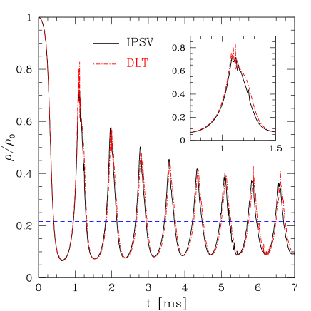
As a side comment we want to point out that we are able to attain higher-than-second order convergence in our results, because the time-step that we use is small enough so that the errors in the spatial discretization are dominating over the errors due to the time evolution, which is only second order.

IV.5 Nonlinear oscillations of spherical stars: the migration test

As a direct extension of the analysis carried in the previous Section on linear oscillations, we next study large nonlinear oscillations which are produced as an equilibrium star model on the unstable branch of equilibria models migrates to the stable branch. This process has been used as a numerical test in 3D codes (see, e.g.  Font et al. (2002); Baiotti et al. (2003, 2005); Cordero-Carrión et al. (2009)), has been analyzed extensively in the past Gourgoulhon (1992); Novak (2001); Noble (2003) and has gained special interest recently when it was shown that it exhibits a critical behaviour Liebling et al. (2010); Radice et al. (2010).

Figure 15: Comparison in the evolution of the normalized central rest-mass density of the migrating star between a simulation in 1D with EDGES (dot-dashed red line), and a simulation in 3D with Whisky (solid black line). Also in this case, the blue dashed line denotes the central rest-mass density of the stable model associated with the initial configuration and the inset shows a magnification of the second peak (see main text for details).

Here, in particular, we have considered a TOV constructed with a polytropic EOS having $K=100$ and $\Gamma=2$, central density $\rho_{c}=7.0\times 10^{-3}$, gravitational mass $M=1.49\,M_{\odot}$ and areal radius $R=6\,M_{\odot}\simeq 8.8$ km. The evolution, on the other hand, was made with an ideal-fluid EOS to properly take into account shock-heating effects. The numerical grid covers the region $0\leq r\leq 30$ and the simulations reported used a polynomial representation of the solution of degree five. Two different stabilization techniques were used. A first one employed an exponential filter of order six with $\mu=40$, applied to the DLTs of the conserved variables and corrected with the “intrinsic” procedure. A second one used instead an IPSV stabilization with $\hat{Q}_{k}=1-\delta_{k0}$ and strength $\mu=1$.

To trigger the migration on the stable branch, the star is perturbed with an outgoing velocity perturbation of the form

$$v(x)=\frac{A}{2}|x^{3}-3x|\,,\quad x=\frac{r}{R}\,,$$ (71)

where $A=0.01$. Under the effect this perturbation the star exhibits a violent expansion and migrates towards a new stable equilibrium configuration with a series of large-amplitude oscillations. During these violent oscillations the exterior layers of the star tend to infall with higher velocity then the interior layers and this leads to the formation of shock waves that heat the neutron star matter and result in the ejection of a small portion of the material of the star.

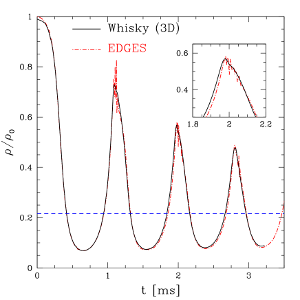
In Fig. 14 we show the evolution of the central density, normalized to its initial value, for two runs employing $150$ elements and different stabilization techniques. Because this test does not have an analytic counterpart, we have compared it the corresponding evolution performed with the Whisky code in a 3D simulation having $N=100$ grid cells in each direction, PPM reconstruction and the HLLE Riemann solver.

Figure 16: Comparison of different stabilization techniques in the migration test. Shown in the two panels is the evolution of the central rest-mass density around the first peak. The left panel refers to a DLT filter on grids of $N=100$ and $N=200$ elements (blue solid and dashed red lines), while the right panel refers the IPSV stabilization technique with $N=100$ and $N=200$ elements (blue solid and cyan long-dashed lines). Note that the DLT-stabilized run reaches convergences with a smaller number of elements.

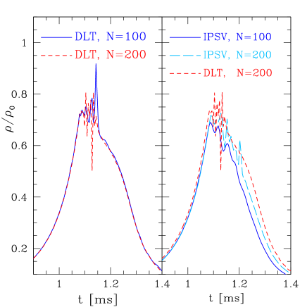
The comparison is offered in Fig. 15 and shows an extremely good agreement. We note that because the two codes have intrinsically different initial truncation errors, the expansion phase in Whisky is slightly delayed with respect to the dynamics produced by EDGES, and we account for this difference by shifting the data obtained by Whisky in order to obtain an approximate alignment at the first minimum of the density. Notwithstanding the very good agreement, the main difference between the two solutions is the presence of high-frequency oscillations in the central density computed by EDGES, and in particular for the DLT runs and near the maximum value of the density. These “spikes” can be tracked down to the propagation of shock waves which are formed in the outer layers of the star during the collapse phase. They have initially a small compression factor, but they also tend to sum up coherently as they travel towards the center, thanks to the assumption of spherical symmetry, so that they result in strong variation of the density near the center of the star. This phenomenon has also been observed in other works in spherical symmetry, employing standard finite-volume schemes, see e.g.  Cordero-Carrión et al. (2009), but is not usually observed in 2D or 3D simulations and, indeed, it is not present in the results obtained with Whisky. In particular Whisky employs Cartesian coordinates, which inevitably introduce preferred directions in the grid, thus preventing the spherical waves produced at the surface from interfering constructively and focussing towards the center. Another reason why these spikes are not observed in multi-dimensional solutions could be related to the larger numerical viscosity due to the necessity of using a much coarser resolution than in the 1D case. This is confirmed by the fact that the use of the IPSV stabilization techniques, which allows us to introduce a much larger numerical dissipation, is able to greatly suppress this phenomenon.

Figure 17: Evolution of the lapse function at the center of an unstable TOV migrating towards the stable branch for two different runs using different stabilization techniques (black solid line for the IPSV stabilization, and red dashed line for the DLT filter) and $N=150$. The inset shows a magnification of the dynamics around the first peak at $1\,\mathrm{ms}$ and highlights that the solution is always smooth.

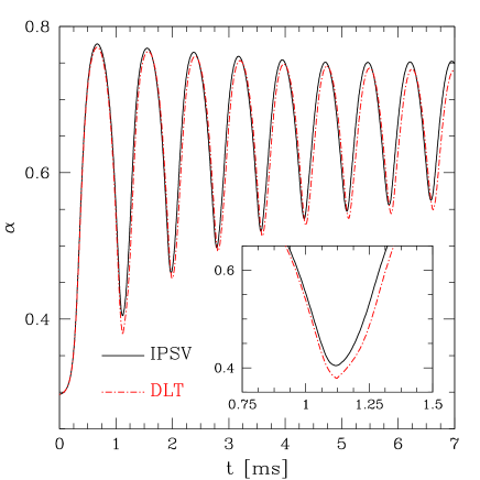
A more detailed comparison between the results obtained with the two stabilization techniques is shown in Fig. 16, where we offer a comparison between the evolution of the central density around the first bounce obtained with the two approaches and with different resolutions. Note that the DLT runs show signs of spikes in the density for all the resolutions (left panel), while the IPSV runs are much smoother (right panel). On the other hand, the results obtained with the DLT filters are already in a convergent regime and in fact the results obtained with $N=100$ elements are very similar to those obtained by doubling the resolution. This is not the case for the solutions obtained with the IPSV filter, that seem to be only slowly approaching the DLT ones (cf. note in the right panel that the IPSV solutions approaches the DLT one as $N$ goes from $100$ to $200$). The evidence that the simulations with the DLT filtering are already in a convergent regime and yet show spikes in the evolution can be interpreted, therefore, as a confirmation that the latter are not a numerical effect, but rather an artifact of the symmetry, which leads to a focusing of the waves travelling towards the center.

Fortunately, because these perturbations actually carry only a very small energy and are amplified by the symmetry, the evolution of the spacetime variables is totally unaffected. This is shown in Fig. 17, where we report the evolution of a particularly representative metric quantity, namely, the lapse function at the center. As can be seen from the figure, the lapse function shows no spikes or spurious oscillation and appears to be smooth with both the DLT and the IPSV filters, the main difference being the value of the minimum attained during the first bounce with the former stabilization technique.

IV.6 Gravitational collapse of unstable spherical stars

As a final test we consider another classical testbed in general-relativistic hydrodynamics: namely, the gravitational collapse to black hole of an unstable TOV star. The problem of the gravitational collapse to a black hole has been already studied in great detail in a number of different conditions involving 1D, 2D and 3D simulations, as well as different physical conditions (see, e.g.  Gourgoulhon (1992); Romero et al. (1996); Novak (2001); Noble (2003); Baiotti et al. (2005); Duez et al. (2006); Baiotti and Rezzolla (2006); Baiotti et al. (2007); Noble and Choptuik (2008); Cordero-Carrión et al. (2010); O’Connor and Ott (2010); Thierfelder et al. (2010)), and has become a standard test of general-relativistic codes. For this reason, we will not discuss the details of the dynamics of the collapse and concentrate instead on the quality of the results obtained with EDGES.

For the tests considered here we have evolved an unstable TOV built with a polytropic EOS with $K=100$ and $\Gamma=2$, having central density $\rho_{c}=4.5\times 10^{-3}$, gravitational mass $M=1.6\,M_{\odot}$ and areal radius $R=6.9\,M_{\odot}\simeq 10.2$ km. In contrast to the migration test, the collapse is triggered by introducing an ingoing velocity perturbation of the type (71) with $A=-0.01$. The evolution of this system is studied on a grid covering $0\leq r\leq 15$, staggered about the origin, using polynomials of degree five and employing an exponential filter of order six, with intrinsic correction and strength $\mu=40$, applied directly on the conserved variables at every time step.

Figure 18: Evolution of the lapse function at the center of an unstable TOV collapsing to a black-hole for different resolutions on. The solid black line, the dotted blue line and the dashed red line are associated with runs employing a grid of $50$, $75$ and $100$ elements, respectively. The inset shows a magnification of the dynamics around $0.6\,\mathrm{ms}$, highlighting some post-collapse dynamics in the lapse for the low-resolution run, which is however absent at higher resolutions.

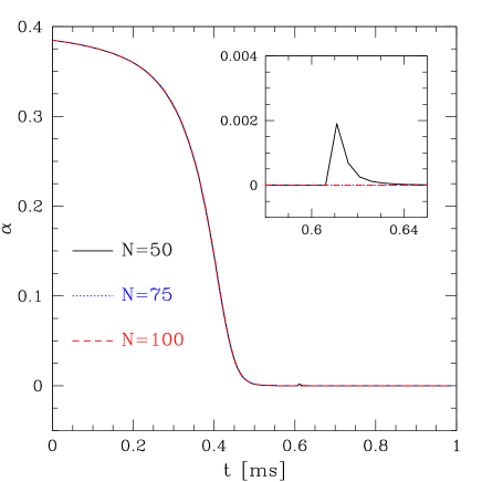
During the evolution and as expected, the central density of the star shows an exponential increase, which halts when the lapse function collapses to zero, signalling the formation of the black hole and “freezing” the evolution in the inner regions of the star. The maximum value attained by the central density does not have any physical meaning, partly because it depends entirely on the gauge conditions and partly because the gauge used will prevent its growth past a certain value. For this reason it is more interesting to look at the evolution of the lapse function at the center of the star, and which we show in Fig. 18. Note that for all the considered resolutions, the lapse function quickly collapses to zero and shows no appreciable subsequent evolution, with the exception of the lowest resolution case, for which a small growth appears again around $0.6\ \mathrm{ms}$. This sudden evolution is the result of errors coming from the surface of the frozen star, where the spatial slice is stretched due to the fact that we fixed our shift gauge condition to zero and, thus, the metric functions present large spatial gradients. These errors, which cannot be compensated by simply increasing the resolution and are a shortcoming of the gauge used, propagate towards the inner regions of the frozen star and can induce a growth of the lapse, restarting the dynamics. This is clearly a resolution-dependent effect which disappears quickly by increasing the resolution (see inset in Fig. 18). Apart from this late-time, and low-resolution dynamics, the three curves are on top of each other, signaling a convergent regime, with a rate we measure to be slightly above the fourth order before the collapse of the lapse. Afterwards the convergence order starts to slowly decay, due to the fact that, as the lapse collapses to zero, the equations are only weakly hyperbolic. At the end of the simulation the convergence order reaches a value which is $\gtrsim 1.5$.

In summary, the solution of the gravitational collapse to a black hole with EDGES has been straightforward and indeed a test which is much less demanding that the migration one, at least in terms of the hydrodynamical variables. The only difficulty encountered is a well known one and has to do with the fact that with such a gauge the collapse of the lapse is not compensated by any change in the shift vector, which is identically zero. As a result, as the black hole is produced it quickly produces a stretching of the coordinates at the location immediately outside the “frozen star”. This, in turn, results in the development of strong gradients in the numerical solution which cannot be resolved indefinitely without suitable adaptivity.

V Conclusions

Numerical, relativistic hydrodynamics and MHD have seen a tremendous growth in the number and the quality of its results after the introduction of modern high-resolution shock capturing schemes Font (2008). These schemes have been proven to be of central importance in the modelling of complex systems involving strong gravity and/or high Lorentz factor. Yet, they suffer from important limitations that ultimately impact the accuracy of the obtained results Baiotti et al. (2009). For this reason the search for better numerical schemes is still on-going (and will always be).

Discontinuous Galerkin schemes were developed to overcome the previously mentioned limitations of finite-volume and finite-difference schemes, while maintaining important properties of these schemes, such as conservation and shock capturing, that made them so successful in a number of applications Cockburn and Shu (2001). For this reason they are a natural candidate as an alternative to more traditional methods also in relativistic hydrodynamics.

In this paper we have developed the necessary mathematical framework needed for the application of discontinuous Galerkin schemes to relativistic hydrodynamics in curved spacetimes. In particular, we have presented both a manifestly covariant weak formulation of relativistic hydrodynamics and a more traditional one obtained within a $3+1$ split. We have then specialized the latter formulation to the spherically symmetric case and implemented it in a new one-dimensional relativistic hydrodynamical code, EDGES, which uses a high-order spectral discontinuous Galerkin method.

The code was tested in a number of situations, including shock waves, spherical accretion, linear and nonlinear oscillations of relativistic spherical stars and the gravitational collapse of unstable stars to black holes. Our results show that discontinuous Galerkin methods are able to sharply resolve shock waves and, at the same time, attain very high, spectral, accuracy in the case of smooth solutions. For this reason they constitute an excellent alternative to classical finite-volume and finite-difference schemes for relativistic hydrodynamics, especially in those situations in which shock waves as well as small-scale features of the flows have to be resolved. In light of the promising prospects shown with these tests and of their affinity with a pseudospectral solution of the Einstein equations, we anticipate that discontinuous Galerkin methods could represent a new paradigm for the accurate modelling in computational relativistic astrophysics.

As a final remark we note that the success of these methods in multi-dimensional implementations will ultimately depend on the development of techniques such as local timestepping, $hp$-adaptivity and load balancing Canuto et al. (2008), which are needed to take full advantage of the flexibility of these schemes Shu (2001). This will represent the focus of our future work.

Appendix A Causal triangulations

In what follows we provide some basic definitions related with the causal structure of the triangulation.

For every open set $A$, we introduce the notation $\partial^{+}A$, to indicate the future boundary of $A$, that is the set of all the points, $p\in\partial A$, such that

$$J^{+}(p)\cap A=\emptyset\,,$$ (72)

$J^{+}(p)$ being the causal future of $p$. Analogously we call past boundary of $A$, $\partial^{-}A$, the set of all the points $p\in\partial A$ for which there exist an open neighborhood, $U$, such that

$$J^{+}(p)\cap U\subset\overline{A}\,,$$ (73)

where we have indicated with $\overline{A}$ the closure of $A$. Finally we will write $\partial^{\times}A$ for $\partial A\setminus[\partial^{+}A\cup\partial^{-}A]$.

For a generic set $E$, instead, the above definitions are modified by considering the interior of the set, $\mathring{E}$. In the case of an element of the grid, $\Omega_{j}$, these definitions are useful to identify the regions of the boundary of $\Omega_{j}$ where the characteristics are always ingoing, $\partial^{-}\Omega_{j}$, always outgoing, $\partial^{+}\Omega_{j}$, or of mixed nature, $\partial^{\times}\Omega_{j}$. These different parts of the causal slice $(I,S)$ containing the element $\Omega_{j}$ are shown in Fig. 19.

We also define as slice of the triangulation, or simply slice, any tuple $(I,S)$ where $I\subset\{1,2,\ldots,N\}$ and $S=\bigcup_{j\in I}\Omega_{j}$ is connected. We will say that a slice $(I,S)$ is a causal slice if

$$\partial^{\times}S\subset\partial\Omega\,.$$ (74)

Figure 19: Schematic representation of a causal slice $(I,S)$ containing the element $\Omega_{j}$. The future and past boundaries $\partial^{\pm}\Omega_{j}$, as well as the time-like or null-like boundaries $\partial^{\times}\Omega_{j}$ of $\Omega_{j}$ are indicated with blue and red lines, respectively. Finally, the shaded region represent the causal slice.

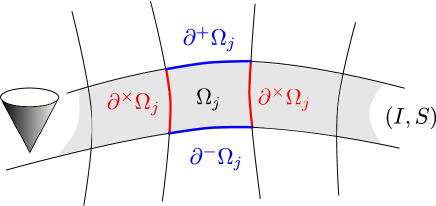
An example of such a slice of the triangulation is given by the shaded region in Fig. 19: a causal slice is basically a slice whose timelike spatial boundaries $\partial^{+}$ and $\partial^{-}$ are parts of a Cauchy foliation of the spacetime. A causal slice $(I,S)$ is said to be a minimal causal slice if it also satisfies the CFL-like condition

$$\Bigg{[}\bigcup_{j\in I}\Big{(}\partial^{\times}\Omega_{j}\cup\partial^{-}\Omega_{j}\Big{)}\setminus\partial\Omega_{k}\Bigg{]}\cap J^{+}(\Omega_{k})=\emptyset,\ \ \forall k\in I,$$ (75)

that is, if the characteristics originating in each element, $\Omega_{k}$, only intersect the boundaries of the element itself, $\partial\Omega$, or the future boundaries of the other elements in the slice.

Finally we say that a triangulation follows the causal structure of the spacetime if it can be written as union of minimal causal slices. Intuitively a triangulation that follows the causal structure of the spacetime is one that can be sliced in minimal causal slices, which are grids associated with a Cauchy foliation of the spacetime and which satisfy a CFL condition on each hyper-surface of this foliation.

If the triangulation $\{\Omega_{j}\}_{j=1}^{N}$ follows the causal structure of the spacetime, in the sense defined above, then we can introduce a family of successive slices $\{(I_{k},S_{k})\}_{k=0}^{Q}$, parametrized by a discrete time $k$, such that $\partial^{-}S_{k+1}\subset\partial^{+}S_{k}\cup\partial\Omega$ and $\Omega=\bigcup_{k}S_{k}$. We can then construct a globally explicit, locally implicit, scheme by solving (9) on the successive slices. The reason is that, for all $j\in I_{k+1}$, the fluxes across $\partial^{-}\Omega_{j}$ and $\partial^{\times}\Omega_{j}$ are completely determined by the data on $S_{k}$ and the boundary conditions, while the fluxes across $\partial^{+}\Omega_{j}$ do not couple $\Omega_{j}$ with other elements within $S_{k+1}$.

Appendix B The continuity equation in the $D=3$ case

We next present an example in which we show in the explicit form the discontinuous Galerkin scheme for the simplest of the equations of relativistic hydrodynamics, namely the continuity equation, and with a polynomial of order $D=3$. In particular we will show the explicit form of the semi-discrete equations for the collocated values in a given element $S_{j}$. In the EDGES code, nodes, weights and interpolating polynomials are always computed numerically. However, for clarity, we are going to present, here, the analytic expressions for the considered case.

The Legendre polynomial of degree three in $[-1,1]$ is given by

$$L_{3}(x)=\frac{1}{2}(5x^{3}-3x),$$

so that the Gauss-Legendre-Lobatto quadrature points, the zeros of $(1-x^{2}){\mathrm{d}L_{3}(x)}/{\mathrm{d}x}$, are

$$\{x_{i}\}_{i=0}^{3}=\{-1,\,-1/\sqrt{5},\,1/\sqrt{5},1\}.$$

The Lagrange polynomials associated with the quadrature points are

$$l_{0}(x) =\frac{1}{8}(1-x)(-1+5x^{2})\,,$$

$$l_{1}(x) =\frac{5}{8}(-1+x)(1+x)(-1+\sqrt{5}x)\,,$$

$$l_{2}(x) =-\frac{5}{8}(-1+x)(1+x)(1+\sqrt{5}x)\,,$$

$$l_{3}(x) =\frac{1}{8}(1+x)(-1+5x^{2})\,,$$

and the associated weights, $w_{i}=\int_{-1}^{1}l_{i}(x)\,\mathrm{d}x$,

$$\{w_{i}\}_{i=0}^{3}=\{1/6,\,5/6,\,5/6,\,1/6\}\,.$$

Dropping now the element index $j$ in the notation of (40), so that for any function $f$, the symbol $f_{i}$ will denote $f\big{(}\varphi_{j}(x_{i})\big{)}$, and restricting ourselves to the continuity equation in $S_{j}$ we find

$$\begin{split}r_{i}^{2}\frac{\mathrm{d}{\cal D}_{i}}{\mathrm{d}t}=&\sum_{k=0}^{4}w_{k}r_{k}^{2}X_{k}v_{k}{\cal D}_{k}\frac{\mathrm{d}l_{i}(x_{k})}{\mathrm{d}x}-\\ &\frac{2}{w_{i}|r_{3}-r_{0}|}\Big{[}r_{0}^{2}X_{0}\mathcal{F}^{-}_{\cal D}\delta_{0i}-r_{3}^{2}X_{3}\mathcal{F}^{+}_{\cal D}\delta_{3i}\Big{]}\,,\end{split}$$ (76)

where $\mathcal{F}_{\cal D}^{\pm}$ denotes the fluxes of ${\cal D}$, between $S_{j}$ and $S_{j\pm 1}$, as obtained by the HLLE solver, i.e.

$$\begin{split}\mathcal{F}^{-}_{\cal D}=\frac{1}{\lambda^{+}-\lambda^{-}}\Big{[}\lambda^{+}(&v_{j-1,3}{\cal D}_{j-1,3})-\lambda^{-}(v_{j,0}{\cal D}_{j,0})\\ &+\lambda^{+}\lambda^{-}({\cal D}_{j-1,3}-{\cal D}_{j,0})\Big{]}\,,\end{split}$$ (77)

and

$$\begin{split}\mathcal{F}^{+}_{\cal D}=\frac{1}{\lambda^{+}-\lambda^{-}}\Big{[}\lambda^{+}(&v_{j+1,0}{\cal D}_{j+1,0})-\lambda^{-}(v_{j,3}{\cal D}_{j,3})\\ &+\lambda^{+}\lambda^{-}({\cal D}_{j+1,0}-{\cal D}_{j,3})\Big{]}\,,\end{split}$$ (78)

where $v_{j,i}\,,{\cal D}_{j,i}$ are the values of $v$ and ${\cal D}$ at the $i$-th collocation point in the $j$-th element and $\lambda^{+}$ and $\lambda^{-}$ are the maximum and minimum characteristic speeds, respectively.

References

- May and White (1966) M. M. May and R. H. White, Phys. Rev. 141, 1232 (1966).
- Wilson (1972) J. R. Wilson, Astrophys. J. 173, 431 (1972).
- Font (2008) J. A. Font, Living Reviews in General Relativity (2008).
- Martí et al. (1991) J. M. Martí, J. M. Ibáñez, and J. A. Miralles, Phys. Rev. D 43, 3794 (1991).
- Banyuls et al. (1997) F. Banyuls, J. A. Font, J. M. Ibáñez, J. M. Martí, and J. A. Miralles, Astrophys. J. 476, 221 (1997).
- Leveque (1992) R. J. Leveque, Numerical Methods for Conservation Laws (Birkhauser Verlag, Basel, 1992).
- Toro (1999) E. F. Toro, Riemann Solvers and Numerical Methods for Fluid Dynamics (Springer-Verlag, 1999).
- Giacomazzo et al. (2011) B. Giacomazzo, L. Rezzolla, and L. Baiotti, Phys. Rev. D 83, 044014 (2011).
- Rezzolla et al. (2011) L. Rezzolla, B. Giacomazzo, L. Baiotti, J. Granot, C. Kouveliotou, and M. A. Aloy, Astrophys. Journ. Lett. 732, L6 (2011).
- Johnsen et al. (2010) E. Johnsen, J. Larsson, A. V. Bhagatwala, W. H. Cabot, P. Moin, B. J. Olson, P. S. Rawat, S. K. Shankar, B. Sjögreen, and H. Yee, Journal of Computational Physics 229, 1213 (2010).
- Baiotti et al. (2009) L. Baiotti, B. Giacomazzo, and L. Rezzolla, Class. Quantum Grav. 26, 114005 (2009).
- Meier (1999) D. L. Meier, The Astrophysical Journal 518, 788 (1999).
- Gourgoulhon (1991) E. Gourgoulhon, Astronomy and Astrophysics 252, 651 (1991).
- Grandclément and Novak (2009) P. Grandclément and J. Novak, Living Reviews in Relativity 12 (2009).
- Bonazzola et al. (1997) S. Bonazzola, E. Gourgoulhon, and J. A. Marck, Phys. Rev. D 56, 7740 (1997).
- Ansorg et al. (2002) M. Ansorg, A. Kleinwächter, and R. Meinel, Astron. Astrophys. 381, L49 (2002), astro-ph/0111080.
- Dumbser and Zanotti (2009) M. Dumbser and O. Zanotti, Journal of Computational Physics 228, 6991 (2009).
- Canuto et al. (2008) C. Canuto, M. Hussaini, A. Quarteroni, and T. Zang, Spectral Methods: Evolution to Complex Gemetries and Applications to Fluid Dynamics (Springer, 2008).
- Cockburn and Shu (2001) B. Cockburn and C.-W. Shu, Journal of Scientific Computing 16, 173 (2001).
- Patera (1984) A. Patera, Journal of Computational Physics 54, 468 (1984).
- Cockburn et al. (2000) B. Cockburn, G. E. Karniadakis, and C.-W. Shu, Discontinuous Galerkin Methods: Theory, Computation and Applications, Lacture Notes on Computational Science and Engineering (Springer, 2000).
- Zumbusch (2009) G. Zumbusch, Classical and Quantum Gravity 26, 175011 (2009).
- Field et al. (2010) S. E. Field, J. S. Hesthaven, S. R. Lau, and A. H. Mroue, Phys. Rev. D 82, 104051 (2010).
- Sopuerta et al. (2006) C. F. Sopuerta, P. Sun, P. Laguna, and J. Xu, Class. Quant. Grav. 23, 251 (2006).
- Sopuerta and Laguna (2006) C. F. Sopuerta and P. Laguna, Phys. Rev. D73, 044028 (2006).
- Dimmelmeier et al. (2005) H. Dimmelmeier, J. Novak, J. A. Font, J. M. Ibáñez, and E. Müller, Phys. Rev. D 71, 064023 (2005).
- Duez et al. (2008) M. D. Duez et al., Phys. Rev. D 78, 104015 (2008).
- Chen et al. (2009) G.-Q. Chen, W. P. Ziemer, and M. Torres, Communications on Pure and Applied Mathematics 62, 242 (2009).
- Chen and Frid (2003) G.-Q. Chen and H. Frid, Communications in Mathematical Physics 236, 251 (2003).
- Palaniappan et al. (2004) J. Palaniappan, R. B. Haber, and R. L. Jerrard, Comput. Methods Appl. Mech. Engrg. 193, 3607 (2004).
- Quarteroni and Valli (1997) A. Quarteroni and A. Valli, Numerical Approximation of Partial Differential Equations (Springer, 1997).
- Papadopoulos and Font (1999) P. Papadopoulos and J. A. Font, Phys. Rev. D 61, 024015 (1999).
- Rezzolla and Miller (1994) L. Rezzolla and J. C. Miller, Classical and Quantum Gravity 11, 1815 (1994).
- Musco et al. (2005) I. Musco, J. C. Miller, and L. Rezzolla, Class. Quantum Grav. 22, 1405 (2005).
- Rosswog (2010) S. Rosswog, Journal of Computational Physics 229, 8591 (2010).
- Siegler and Riffert (2000) S. Siegler and H. Riffert, The Astrophysical Journal 531, 1053 (2000).
- Romero et al. (1996) J. V. Romero, J. M. Ibáñez, J. M. Martí, and J. A. Miralles, Astrophys. J. 462, 839 (1996).
- Noble (2003) S. C. Noble, A Numerical Study of Relativistic Fluid Collapse, Ph.D. thesis, University of Texas at Austin (2003), gr-qc/0310116v1 .
- Yang (2000) D. Yang, C++ and Object-Oriented Numeric Computing for Scientists and Engineers (Springer-Verlag, 2000).
- Veldhuizen (1998) T. L. Veldhuizen, in Proceedings of the Second International Symposium on Computing in Object-Oriented Parallel Environments, ISCOPE ’98 (Springer-Verlag, London, UK, 1998) pp. 223–230.
- (41) http://www.oonumerics.org/blitz/.
- Davis (2002a) T. A. Davis, A column pre-ordering strategy for the unsymmetric-pattern multifrontal method, Tech. Rep. TR-02-001 (Univ. of Florida, CISE Dept., Gainesville, FL, 2002).
- Davis (2002b) T. A. Davis, Algorithm 8xx: UMFPACK V3.2, an unsymmetric-pattern multifrontal method with a column pre-ordering strategy, Tech. Rep. TR-02-002 (Univ. of Florida, CISE Dept., Gainesville, FL, 2002) (http://www.cise.ufl.edu/tech-reports. Submitted to ACM Trans. Math. Softw.).
- Davis and Duff (1997) T. A. Davis and I. S. Duff, SIAM J. Matrix Anal. Applic. 18, 140 (1997).
- Davis and Duff (1999) T. A. Davis and I. S. Duff, ACM Trans. Math. Softw. 25, 1 (1999).
- (46) T. A. Davis, “UMFPACK: A set of routines for solving sparse linear systems via LU factorization,” UMFPACK.
- Gottlieb et al. (2009) S. Gottlieb, D. Ketcheson, and C.-W. Shu, Journal of Scientific Computing 38, 251 (2009), 10.1007/s10915-008-9239-z.
- Gottlieb and Tadmor (1991) D. Gottlieb and E. Tadmor, Mathematics of Computation 56, 565 (1991).
- Arnold (1982) D. N. Arnold, SIAM J. Numer. Anal. 19, 742 (1982).
- Arnold et al. (2002) D. N. Arnold, F. Brezzi, B. Cockburn, and L. D. Marini, SIAM J. Numer. Anal. 39, 1749 (2002).
- Saad (1996) Y. Saad, Iterative Methods for Sparse Linear Systems (SIAM, 1996).
- Biswas et al. (1994) R. Biswas, K. D. Devine, and J. E. Flaherty, Applied Numerical Mathematics 14, 255 (1994).
- Krivodonova (2007) L. Krivodonova, Journal of Computational Physics 226, 879 (2007).
- Maday et al. (1993) Y. Maday, S. M. O. Kaber, and E. Tadmor, SIAM J. Numer. Anal 30, 321 (1993).
- Canuto et al. (1988) C. Canuto, M. Y. Hussani, A. Quarteroni, and T. A. Zang, Spectral Methods in Fluid Dynamics, 2nd ed. (Springer-Verlag, New York and Berlin, 1988).
- Hesthaven and Kirby (2008) J. S. Hesthaven and R. M. Kirby, Math. Comput. 77, 1425 (2008).
- Meister et al. (2009) A. Meister, S. Ortleb, and T. Sonar, “On spectral filtering for discontinuous Galerkin methods on unstructured triangular grids,” (2009), http://cms.uni-kassel.de/unicms/fileadmin/groups/w_180000/prep/prep0904.pdf.
- Boyd (1996) J. P. Boyd, in Proceedings of the Third International Conference on Spectral and High Order Methods, edited by L. R. S. A. V. Illin (Houston Journal of Mathematics, 1996) pp. 267–276.
- Galeazzi (2008) F. Galeazzi, Modelling fluid interfaces in numerical relativistic hydrodynamics, Master’s thesis, Università degli studi di Padova (2008).
- Kastaun (2006) W. Kastaun, Phys. Rev. D 74, 124024 (2006).
- Millmore and Hawke (2010) S. T. Millmore and I. Hawke, Classical and Quantum Gravity 27, 015007 (2010).
- Font et al. (2002) J. A. Font, T. Goodale, S. Iyer, M. Miller, L. Rezzolla, E. Seidel, N. Stergioulas, W. M. Suen, and M. Tobias, Phys. Rev. D 65, 084024 (2002).
- Baiotti et al. (2005) L. Baiotti, I. Hawke, P. J. Montero, F. Löffler, L. Rezzolla, N. Stergioulas, J. A. Font, and E. Seidel, Phys. Rev. D 71, 024035 (2005).
- Gabler et al. (2009) M. Gabler, U. Sperhake, and N. Andersson, Phys. Rev. D 80, 064012 (2009).
- Wang (2002) Z. Wang, Journal of Computational Physics 178, 210 (2002).
- Touil et al. (2007) H. Touil, M. Hussaini, and M. Sussman, J. Comput. Phys. 225, 1810 (2007).
- Berger et al. (2005) M. Berger, M. J. Aftosmis, and S. M. Murman, Analysis of Slope Limiters on Irregular Grids, NAS Technical Report 2005-0490 (American Institute of Aeronautics and Astronautics, 2005).
- Martí and Müller (2003) J. M. Martí and E. Müller, Living Rev. Relativ. 6, 7 (2003).
- Del Zanna et al. (2007) L. Del Zanna, O. Zanotti, N. Bucciantini, and P. Londrillo, Astron. Astrophys. 473, 11 (2007).
- Suresh and Huynh (1997) A. Suresh and H. T. Huynh, Journal of Computational Physics 136, 83 (1997).
- Zhou et al. (2001) T. Zhou, Y. Li, and C.-W. Shu, Journal of Scientific Computing 16, 145 (2001).
- Noh (1987) W. Noh, Journal of Computational Physics 72, 78 (1987).
- Rider (2000) W. Rider, Journal of Computational Physics 162, 395 (2000).
- Michel (1972) F. C. Michel, Astrophys. Spa. Sci. 15, 153 (1972).
- Tooper (1965) R. F. Tooper, Astrophysical Journal 142, 1541 (1965).
- Yoshida and Eriguchi (2001) S. Yoshida and Y. Eriguchi, Mon. Not. R. Astron. Soc. 322, 389 (2001).
- Agrez (2007) D. Agrez, IEEE Transactions on Instrumentation and Measurement 56, 2111 (2007).
- Cerda-Duran (2009) P. Cerda-Duran, “Numerical viscosity in hydrodynamics simulations in general relativity,” (2009), 0912.1774v2 .
- Giacomazzo and Rezzolla (2007) B. Giacomazzo and L. Rezzolla, Class. Quantum Grav. 24, S235 (2007).
- Pollney et al. (2007) D. Pollney, C. Reisswig, L. Rezzolla, B. Szilágyi, M. Ansorg, B. Deris, P. Diener, E. N. Dorband, M. Koppitz, A. Nagar, and E. Schnetter, Phys. Rev. D 76, 124002 (2007).
- Schnetter et al. (2004) E. Schnetter, S. H. Hawley, and I. Hawke, Class. Quantum Grav. 21, 1465 (2004).
- Dimmelmeier et al. (2002) H. Dimmelmeier, J. A. Font, and E. Müller, Astron. Astrophys. 388, 917 (2002).
- Baiotti et al. (2003) L. Baiotti, I. Hawke, P. Montero, and L. Rezzolla, in Computational Astrophysics in Italy: Methods and Tools, Vol. 1, edited by R. Capuzzo-Dolcetta (MSAIt, Trieste, 2003) p. 210.
- Cordero-Carrión et al. (2009) I. Cordero-Carrión, P. Cerdá-Durán, H. Dimmelmeier, J. L. Jaramillo, J. Novak, and E. Gourgoulhon, Phys. Rev. D 79, 024017 (2009).
- Gourgoulhon (1992) E. Gourgoulhon, Classical and Quantum Gravity 9, S117 (1992).
- Novak (2001) J. Novak, Astron. Astrophys. 376, 606 (2001).
- Liebling et al. (2010) S. L. Liebling, L. Lehner, D. Neilsen, and C. Palenzuela, Phys. Rev. D 81, 124023 (2010).
- Radice et al. (2010) D. Radice, L. Rezzolla, and T. Kellerman, Classical and Quantum Gravity 27, 235015 (2010).
- Duez et al. (2006) M. D. Duez, Y. T. Liu, S. L. Shapiro, M. Shibata, and B. C. Stephens, Phys. Rev. Lett. 96, 031101 (2006).
- Baiotti and Rezzolla (2006) L. Baiotti and L. Rezzolla, Phys. Rev. Lett. 97, 141101 (2006).
- Baiotti et al. (2007) L. Baiotti, I. Hawke, and L. Rezzolla, Class. Quantum Grav. 24, S187 (2007).
- Noble and Choptuik (2008) S. C. Noble and M. W. Choptuik, Phys. Rev. D 78, 064059 (2008).
- Cordero-Carrión et al. (2010) I. Cordero-Carrión, P. Cerdá-Durán, and J. María Ibáñez, Journal of Physics Conference Series 228, 012055 (2010).
- O’Connor and Ott (2010) E. O’Connor and C. D. Ott, Classical and Quantum Gravity 27, 114103 (2010).
- Thierfelder et al. (2010) M. Thierfelder, S. Bernuzzi, D. Hilditch, B. Bruegmann, and L. Rezzolla, Phys. Rev. D 83, 064022 (2010).
- Shu (2001) C. W. Shu, High order finite difference and finite volume WENO schemes and discontinuous Galerkin methods for CFD, Tech. Rep. ICASE Report 2001-11; NASA CR-2001-210865 (NASA Langley Research Center, 2001).