∎ \thankstexte1e-mail: waleed.elhanafy@bue.edu.eg \thankstexte2e-mail: nashed@bue.edu.eg 11institutetext: Centre for theoretical physics, the British University in Egypt, 11837 - P.O. Box 43, Egypt 22institutetext: Mathematics Department, Faculty of Science, Ain Shams University, Cairo, Egypt 33institutetext: Egyptian Relativity Group, Egypt
The Hidden Flat Like Universe
Abstract
We study a single fluid component in a flat like universe (FLU) governed by gravity theories, where is the teleparallel torsion scalar. The FLU model, regardless the value of the spatial curvature , identifies a special class of gravity theories. Remarkably, the FLU gravity does not reduce to teleparallel gravity theory. In large Hubble spacetime the theory is consistent with the inflationary universe scenario and respects the conservation principle. The equation of state (EoS) evolves similarly in all models . We study the case when the torsion tensor is made of a scalar field, which enables to derive a quintessence potential from the obtained gravity theory. The potential produces Starobinsky-like model naturally without using a conformal transformation, with higher orders continuously interpolate between Starobinsky and quadratic inflation models. The slow-roll analysis shows double solutions so that for a single value of the scalar tilt (spectral index) the theory can predict double tensor-to-scalar ratios of -mode and -mode polarizations.
1 Introduction
The general relativity (GR) theory explained the gravity as spacetime curvature. This description of gravitation has succeeded to confront astrophysical observations for a long time. It has predicted perfectly the perihelion shift of Mercury, time delay in the solar system. Even in the strong field regimes such as binary pulsars it has amazingly predicted their orbital decay due to gravitational radiation by the system. While it fails to predict the accelerating cosmic expansion which is evidenced by the astronomical observations of high-redshift Type Ia supernovae SN98 . The teleparallel equivalent of general relativity (TEGR) theory has provided an alternative description of Einstein’s gravity. The theory constructed from vierbein (tetrad) fields111The Greek letters denote the spacetime indices and the Latin ones denote Lorentz indices. Both run from to . instead of metric tensor fields . The metric space, however, can be constructed from the vierbein fields, so the Levi-Civita symmetric connection . It is, also, possible to construct Weitzenböck nonsymmetric connection . The first connection has a non-vanishing curvature tensor but a vanishing torsion tensor , while the later is characterized by a vanishing curvature tensor but a non-vanishing torsion tensor . The combined picture could be encoded in the contracted Bianchi identity
where is the usual Ricci scalar, the scalar invariant is called the teleparallel torsion scalar (it will be briefly investigated in Section 2 and the covariant derivative is with respect to (w.r.t.) the Levi-Civita connection. The variation of the left hand side w.r.t. the metric tensor provides the GR field equations. Since the last term in the identity is a total derivative, it does not contribute to the field equations, and the variation of the right hand side w.r.t. the vierbein fields provides a set of field equations equivalent to the GR that is called TEGR. Although the two theories are quantitatively equivalent at their level of the field equations, they are qualitatively different at the level of their actions! Indeed, the total derivative term is scalar invariant under diffeomorphism but not invariant under local Lorentz transformation (LLT). On the other hand, the Ricci scalar in Einstein-Hilbert action leads to a theory invariant under diffeomorphism as well as LLT. Consequently, the teleparallel torsion scalar is not invariant under LLT AP2013 . The absence of local Lorentz symmetry in TEGR action will not be reflected in the field equations, so it does not worth to worry about it. However, the presence of the total derivative term is crucial when consider the extension of TEGR 1010.1041 ; 1012.4039 .
The telleparallel geometry has received attentions in the last decade. However, this geometry has been used very earlier in 1920s to unify gravity and electromagnetism by Einstein E28 . After this trial the geometry has been developed M52 ; MM56 ; M64 . Later, successful extensions to Einstein’s work allowed a class of theories with a quadratic torsion in Lagrangian density MW77 ; M78 ; HS79 . Other trials to obtain a gauge field theory of gravity using the teleparallel geometry have shown a great interest U56 ; K61 ; S64 ; H76 ; U80 . Recent developments attempted a global approach by using arbitrary moving frames instead of the local expressions in the natural basis NS07 ; NS13 . Also, it worths to mention other developments to the teleparallel geometry by imposing Finslerian properties to this geometrical structure W09 ; WK11 ; YST12 . Actually, this geometry provides an alternative tool for deeper studies of the gravity.
An interesting variant of the TEGR is the Born-Infeld-modified teleparallel gravity. Within this framework the early cosmic acceleration (inflation) could be accounted for with no need to an inflaton field FF07 ; FF08 . Another remarkable variant on generalizations of TEGR are the theories similar to the extensions of Einstein-Hilbert action. Within this new class of modified gravity theories a particular form has been proposed to explain the late-time cosmic speeding up without dark energy (DE) BF09 ; L10 ; 1008.4036 ; 1011.0508 . As is well known that theories are conformally equivalent to Einstein-Hilbert action plus a scalar field. In contrast, the theories cannot be conformally equivalent to TEGR plus a scalar field Y2011 . Short period these pioneering studies have been followed by a large number of papers exploring different aspects of the gravity in astrophysics CDDS11 ; FF011 ; FF11 ; IS12 ; CGS13 ; Nashed1 ; Nashed2 ; RHTMM13 ; Nashed3 ; BFG15 ; Nashed4 ; Nashed5 and in cosmology 1205.3421 ; BNO14 ; BO14 ; JMM14 ; HLOS14 ; NH14 ; WH14 ; HN14 ; 1503.05281 ; 1503.07427 . Some applications show interesting results, e.g. avoiding the big bang singularity by presenting a bouncing solution CCDDS11 ; CQSW14 . Also, a graceful exit inflationary model within the cosmology has been argued in NHS14 . A recent promising variant is the modified teleparallel equivalent of Gauss-Bonnet gravity and its applications KS114 ; KS214 ; KS314 .
Spatially flat universe (SFU), i.e. , is used widely in the literature seeking for consistency with cosmic observations. However, recent observations by Planck satellite suggest, also, an open universe as a reliable model Pl2 . On the other hand, the smallness of the curvature density parameter cannot be covered by SFU assumption. In the present study, instead of restrict ourselves to SFU, we impose FLU assumptions into the modified Friedmann equations. This model identifies a hidden class of gravity theories that cannot be covered by assuming a SFU. The rest of this paper is structured as follows: In Section 2, we briefly review the teleparallel geometry and the gravity theories. In Section 3, we use the modified version of the Friedmann equations according to gravity to describe a FLU. In Section 4, we discuss the physical and cosmological consequences of the obtained results. In Section 5, we assume the case when the torsion tensor is made of a scalar field. This enables to construct an exact inflation model powered by a quintessence like field sensitive to the spacetime symmetry. In addition, it enables to induce a generalized Starobinsky potential from the obtained gravity theory. In Section 6, we study possible solutions of the slow-roll parameters of this theory. We discuss testable predictions of the theory according to the recent released Planck and BICEP2 data Pl1 ; Pl2 ; BICEP2 . The work is summarized in Section 7.
2 Extended Teleparallel Gravity
In what follows, we give the structure of Weitzenböck -space. It is described as a pair , where is a -dimensional smooth manifold and () are -linearly independent vector (vierbein) fields defined globally on . Consequently, the is nonzero. The vierbein fields and their dual coframes are orthonormal, i.e. and , where is the Kronecker tensor. The metric space can be constructed from the vierbein fields where is the Minkowski metric for the tangent space, so the Riemannian geometry is recovered. It is, also, possible to construct Weitzenböck nonsymmetric connection
| (1) |
where . The Weitzenböck space is characterized by the vanishing of the vierbein’s covariant derivative, i.e.
| (2) |
where the covariant derivative is w.r.t. the Weitzenböck connection. So this property identifies auto parallelism or absolute parallelism condition. As a matter of fact, the operator is not covariant under local Lorentz transformations (LLT) allowing all LLT invariant geometrical quantities to rotate freely in every point of the space M2013 . In this sense, the symmetric metric (10 degrees of freedom) cannot predict exactly one set of vierbein fields; then the extra six degrees of freedom of the 16 vierbein fields need to be fixed in order to identify exactly one physical frame. The frames are called the parallelization vector fields. It can be shown that the teleparallelism condition (2) implies the metricity condition . The Weitzenböck connection (1) is curvature free while it has torsion tensor. The torsion and the contortion tensor fields of type (1,2) in spacetime coordinates are
| (3) | |||||
| (4) |
In the teleparallel space one may define three Weitzenböck invariants: , and , where . We next define the invariant , where , and are arbitrary constants M2013 . For the values: , and the invariant is just the Ricci scalar , up to a total derivative term as mentioned in Section 1; then a teleparallel version of gravity equivalent to GR can be achieved. The teleparallel torsion scalar is given in the compact form
| (5) |
where the superpotential tensor is defined as
| (6) |
which is skew symmetric in the last two indices. Similar to the theory one can take the action of theory as
| (7) |
where is the reduced Planck mass, which is related to the gravitational constant by . Assuming the units in which , in the above equation and are the matter fields. The variation of (7) w.r.t. the tetrad field requires the following field equations BF09
| (8) |
where , , and is the energy-momentum tensor.
3 Cosmological Modifications of
We first assume that our universe is an isotropic and homogeneous, which directly gives rise to the tetrad field given by Robertson R32 . This can be written in spherical polar coordinate (, , , ) as follows:
| (13) |
where is the scale factor, and . The tetrad (13) has the same metric as FRW metric
3.1 Modified Friedmann equations
Applying the field equations (2) to the FRW universe (13), assuming an isotropic perfect fluid the energy-momentum tensor takes the form . The field equations (2) read
| (15) |
| (16) | |||||
where identifies the spatial coordinate running from , , and is the Hubble parameter, the dot denotes the derivative w.r.t. cosmic time . Equations (15) and (16) are the modified Friedmann equations in the gravity. Substituting from the vierbein (13) into (5), we get the torsion scalar
| (17) | |||||
where is called the curvature density parameter. In above, the modified Friedmann equations might show interesting results since the first round bracket in (16) is the additive inverse of (15). This provides a good chance to hunt a cosmological constant like matter perfectly, if the extra terms of (16) vanish. However, these terms enable evolutions away from the cosmological constant. By careful look to (16) we find that these extra quantities can be split into a free term and dependent term222One should note that may contain dependent quantities.. Taking the SFU assumption leads to disappearance of the last term in (16); then the chance for hunting cosmological constant like DE is by taking the highly restrictive condition or by taking its coefficient . Since we are dealing within the SFU framework, hence the teleparallel torsion scalar (17) can be related to Hubble parameter by . Only the SFU identifies a particular class of . In this article we take a different path allowing evolution away from the cosmological constant without assuming spatial flatness, but enforcing the evolution to be flat like model.
3.2 Searching for a flat like universe
Most cosmological models assume SFU models seeking for a perfect match with cosmological observations. As a matter of fact, taking the spatial flatness as a firm prediction of inflation is not quite accurate. It is easy to show that the smallness of can be a reflection of as expected at early universe. It has been shown that even with a relatively large curvature parameter one can gain all advantages of inflation. On the other hand, it has been shown that the curvature density parameter average is at confidence FMR15 . Moreover, it has been shown that the so-called modified growth parameters are correlated with the curvature density parameter with a recognizable deviation at , which leads some to conclude that the spatial curvature must be included in the analysis with other cosmological parameters DI12 ; NH14 ; ZZCZ14 ; HN14 . Recalling the modified Friedmann equations (15) and (16), we allow the fluid to evolve away from the cosmological constant like fluid regardless the value of . Instead of taking the constraint of the SFU model, we assume the vanishing of the coefficient of in (16) so that
| (18) |
The FLU model ansatz (18) identifies a hidden special class of gravity theories which cannot be covered by taking SFU model. The solution of (18) is not easy in non-flat models. Also, it worths to mention that this treatment cannot be applied in the TEGR theory, i.e. , since the coefficient of in (16) is a constant. So it would not provide us with a condition similar to (18) for examining a FLU. In this case one is obliged to assume a global spatial flatness by putting to study flat universe model. Thus we expect that the FLU treatment enables to study gravity beyond the TEGR or GR domains. As in FRW spacetime is a function of time , one easily can show that
| (19) |
Substituting from (19) into (18), then solve to we get:
| (20) |
where and are integration constants. We later show that the constant can be perfectly interpreted as cosmological constant. In order to reduce the dependence on , we follow the same ansatz (18) by taking a vanishing value of the coefficient of . So, in the above equation, we take
| (21) |
by solving for we get the scale factor
| (22) |
where is an arbitrary constant of integration, with an initial condition . One should mention that the scale factor is independent of the choice of . On the other hand, we do not expect or accept that the three world models to be completely coincide, then the function should depend on the choice of in its final form. Substituting from (22) into (17) we get the torsion scalar
| (23) |
Substituting from (22) into (20) and expanding the exponential around ; then the is obtained as a function of as
| (24) |
where are constant coefficients consist of the set of constants . The zeroth term of (24) derives the Friedmann equations (15) and (16) to produce the cosmological constant DE, so fixes the value of the coefficient to the cosmological constant. We give examples of the coefficients: , , , … etc, where . The higher orders of the expansion in (24) produce the evolution away from the cosmological constant. Equation (23) enables to write the time mathematically in terms of the torsion scalar, i.e. ; then we reexpress (24) in terms of the torsion scalar as inverse power law of as333We give the in terms of the torsion scalar to explore the in its usual form. But all the calculations in this work are performed using the time dependent form (24).
where are known constant coefficients consist of the same set of constants similar to the coefficients . The above expression shows that does not reduce to TEGR as expected so that it describes a non ordinary matter. Accordingly, we cannot assume a fixed EoS as in the classical cases. But it is more convenient to consider the case of the time dependent EoS corresponds to the contribution of the dynamical evolution of the to the density and pressure. We summarize the FLU model as below:
-
(a)
In the GR theory, a fixed value of the equation of state (EoS) parameter, , is entered to the Friedmann equations as an input; then the scale factor is obtained as an output.
-
(b)
In the theories, a fixed EoS parameter in addition to a scale factor are entered to the Friedmann equations as inputs; then an is obtained as an output.
- (c)
In the (c) case, the FLU constrains the scale factor and by the model assumptions. These assumptions allow density and pressure to reformulate accordingly as functions of time. So it is not convenient to add an extra condition, e.g. assuming a fixed EoS. Whereas the EoS in the FLU model should be treated as a time dependent output parameter, i.e. , this grantees a consistent system of Friedmann equations. Actually, the only thing that we have to worry about, in of cosmological applications, is obtaining compatible and NH14 . It worths to mention that the fine tuning problem facing DE models with a constant equation of state can be alleviated if we assume that the EoS is time dependent, e.g. quintessence models S02 . So one should think of this model as quintessence models rather than classical cosmological models.
4 Cosmic Evolution
In this Section, we perform a cosmological study of the FLU model to examine its capability to obtain the cosmic evolution. In addition, we study its consistency with the Friedmann equations. The FRW spacetime that is governed by gravity can be determined by a scale factor and an form. As we mentioned before that the scale factor (22) is independent of , while the , namely (24), depends on as it should be. This allows to study different evolution scenarios according to the choice of , assuming that the FRW universe is filled with a single fluid component given by (15) and (16), we examine the cosmic evolution as follows.
4.1 The large Hubble-spacetime
We study the large -regime, i.e. at early time universe. The Hubble parameter corresponds to the scale factor (22) is given by
| (25) |
where the modified Friedmann equations are symmetric under . We easily find that the universe is always accelerating as the deceleration parameter . Nevertheless, the matter density (15) of this theory in the large -spacetime is given as , which agrees with the predictions of the vacuum density with a correction term. This is consistent with the inflationary universe scenario at this stage.
4.2 Single-fluid equation of state
In this theory, we assume only a single fluid component to describe the matter of the universe. As we mentioned in Subsection 3.2, there is a good chance to hunt negative pressure matter in the framework with expected deviation from the cosmological constant behaviour. We now examine the nature of this single-fluid component and its possible evolution. Using (15) and (16), we get a time dependent EoS parameter (). The dynamical behaviour shows a similar asymptotic behaviour regardless the universe is flat or not. It is only affected by the order of expansion of (24). We need to mention that the shows that the leading term producing an EoS as a constant function of time , which describes the cosmological constant DE perfectly. However, the value of does not necessarily large as we will see later. We choose initial conditions to fit with the early universe, by taking a tiny initial scale factor combined with a large initial Hubble constant at Planck time . When the first order correction is taken into consideration, the EoS approaches as , where is time large enough at which the EoS gets its final steady phase. While the second order correction allows the EoS to evolve up to as . We conclude that the series of the up to the second order correction does not allow the EoS to crossover at anytime. These cases of are useful to describe the very early universe.
We give the model more attention as it produces an excellent agreement with the acceptable cosmic evolution scenario, see the plots of Figure 1. Although, we used a single-fluid component, its dynamical evolution allows the EoS parameter initially to start from (phantom). The evolution of the EoS shows almost the same behaviour in the three models. Then it evolves to pressureless cold dark matter (CDM) (), radiation () and possibly stiff-matter (), while it shows a quintessence fate as in all models. This shows a unique origin of early and late cosmic accelerating expansion. So we find that the third order correction is the most physical scenario. In the cases of , we have a physical motivation to study the series up to only as the EoS of higher order produces asymptotically which represents unknown matter so far.
We find that the EoS asymptotic behaviour increases by a quantized value as , , , as the -th order increases by unity in the series (24).
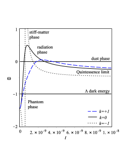
It worths to mention that the FLU model shares the quintessence models an important result, a dynamical EoS. In addition, the theory predicts similar evolutions at early time in the three models . Moreover, it forces the flat/non-flat models to have identical behaviours at a later time. Thus, the FLU model succeeds to describe an effectively flat solution without imposing a global vanishing sectional curvature by taking .
4.3 Conservative universe
As mentioned in the introduction of the present Section that we extract a scale factor (22) and an (24) as solutions of two assumptions (20) and (21) of the FLU model, not directly from Friedmann equations as usual. We examine the validity of the Friedmann equations for this model. Actually, the case of the cosmological constant with a fixed EoS parameter () that is required to describe the accelerating universe, one cannot get an evolutionary scenario for this dark component. In addition, its continuity equation
| (26) |
shows that , i.e. density is constant. Nevertheless, the density should decreases as universe expands. This conflict implies a continuous creation of matter in order to keep the density of the expanding universe constant. This case is similar to the steady state cosmology which breaks the conservation principle. This problem vanishes as a consequence of assuming a dynamical EoS as in our case here of the FLU model. In this theory, we use one fluid component to describe the evolution of the universe, with a negative pressure matter dominating most of different epochs during the early time evolution. Moreover, we get a conservative universe. This can be obtained by substituting from (22) and (24) into (15) and (16), which shows that the continuity equation is always verified up to any order of expansion of (24).
We summarize the results of Section 4 as follows: The FLU model (i) is consistent with inflationary scenario universe, (ii) has dynamical EoS parameter allows cosmic evolution, and (iii) satisfies the continuity equation so Friedmann. It is well known that the scalar field plays the key role in the quintessence models to interpret the inflation stage at early universe. On the other hand, the torsion plays the main role in the teleparallel geometry. We next consider the role of the torsion as added value quality of the spacetime when formed by a scalar field and its role at the early universe time.
5 Torsion Potential
In order to get the idea of the torsion potential, we first discuss the physical meaning of the connection coefficients as the displacement field. So we use (4) to reexpress the Weitzenböck connection (1) as
| (27) |
By careful look to the above expression of the new displacement field, it consists of two terms. The first is the Levi-Civita connection which consists of the gravitational potential (metric coefficients, ) and its first derivatives w.r.t. the coordinates. Where the second term is the contortion which consists of the tetrad field and its first derivatives w.r.t. the coordinates. In this sense we find the first term contributes to the displacement field as the usual attractive force of gravity, while the second term contributes as a force too. While equation of motion tells that this force is repulsive W2012 . Now we can see how teleparallel geometry adds a new quality (torsion or contortion) to the spacetime allowing repulsive side of gravity to showup.
5.1 Torsion potential of a scalar field
We consider here the physical approach to construct the torsion from a scalar field . In the view of the above discussion, we can treat the contortion in the Weitzenböck connection (27) as a force. Accordingly, it is required to construct the contortion (or torsion) from a tensor and it first-order derivatives. Then, this tensor now plays the role of the potential of the torsion. We follow the approach that has been proposed by XSH96 , by introducing sixteen fields that are called torsion potential. These fields form a quadruplet basis vectors, so we write the following linear transformation:
the torsion potential and its inverse are satisfying the conditions:
Finally, this enables to express the torsion as XSH96
| (28) |
The torsion potential can be reformed by a physical scalar, vector or tensor fields. This may have a great interest in physical applications. Now we take the case when the torsion potential is formed by a scalar field by taking
| (29) |
where is a non-vanishing scalar field. Then the torsion and the contortion (4) can be reexpressed respectively as
| (30) | |||||
| (31) |
where . The above expressions have been used in order to formulate a theory of the electromagnetism minimally coupled to torsion and satisfies gauge invariance and minimal coupling principles R74 ; HRR78 ; H90 ; HO01 . Using (6), (30) and (31), the teleparallel torsion scalar (5) can be written in terms of the scalar field as
| (32) |
The above treatment shows that the torsion acquires dynamical properties and it propagates through space. It worths to mention that the energy momentum tensor of a free scalar field represents a source of the dynamical torsion in the teleparallel description of gravity AP98 , which is not in agreement with the common belief that the spin matter only can produce torsion H76 . One should mention here that same results can be achieved by combining the conformal transformation of the tetrad fields and in addition to the so-called Einstein -transformation (projective transformation) of the connection coefficients E55 ; FRM13 as
| (33) |
Actually, this approach, indeed, has a geometrical framework as well. Where the connection is assumed to be a semi-symmetric one, this case has been studied by many authors, c.f. NA2005 .
5.2 Gravitational quintessence model
It is well known that the cosmic inflation is powered by a scalar field . On the other hand, the cosmological applications of gravity show strong evidences of a cosmic inflation. So there must be a link between these two descriptions, we see that equation (32) provides this link as the teleparallel torsion scalar appears as a gradient of a scalar field. So it acquires dynamical properties and propagates through space. Also, equation (32) enables us to map the density and pressure contributions in the Friedmann equations into the scalar field (, ). This leads to reformulate the Friedmann equations of the torsion contribution as an inflationary background in terms of the scalar field . As mentioned before the FLU model provides does not reduce to TEGR theory of the ordinary matter. This is in agreement with the inflationary epoch where the matter contribution can be negligible. Accordingly, we consider the Lagrangian density of a homogeneous (real) scalar field in potential
| (34) |
where the first expression in (34) represents the kinetic term of the scalar field, as usual, while represents the potential of the scalar field. The variation of the action w.r.t. the metric enables to define the energy momentum tensor as
The variation w.r.t. the scalar field reads the scalar field density and pressure respectively as
| (35) |
The Friedmann equation (15) of the non-flat models in absence of matter becomes
Using (35) it is an easy task to show that continuity equation (26) reduces to the Klein-Gordon equation of homogeneous scalar field in the expanding FRW universe
where the prime denotes the derivative w.r.t. the scalar field . In conclusion, equation (32) enables to define a scalar field sensitive to the vierbein field, i.e. the spacetime symmetry. In addition, equation (35) enables to evaluate an effective potential from the adopted gravity theory. The mapping from the torsion contribution to scalar field fulfills the Friedmann and Klein-Gordon equations. So the treatment meets the requirements to reformulate the torsion contribution in terms of a scalar field without attempting a conformal transformation.
5.3 Generalized Starobinsky potential by
In the following treatment, we take the simple case of the flat space universe in order to compare the obtained results to the standard treatment of the scalar field theory in cosmology. Using (23), (32) we get
| (36) |
where is as given in Subsection 3.2. Integrating the above equation we write the scalar field as
| (37) |
and is a constant of integration. The above equation allows to express the time mathematically in terms of the scalar field . So all the dynamical expressions can be expressed in terms of the scalar field.
The relation between the scalar fields and has to be investigated. Using (23) and (37) we can express the torsion scalar field in terms of the scalar field as
| (38) |
As is well known at the strong coupling condition the inflaton field is related to the canonical scalar field by KLR214
| (39) |
Comparing the above equation with the teleparallel torsion (38) we get the transformation where the constant can be absorbed in the coefficient . This indicates that the teleparallel torsion scalar might play a role similar to the canonical scalar field normally used in scalar-tensor theories of gravitation. Also, using (22) and (24), the pressure (16) can be reexpressed in terms of the scalar field as
| (40) |
where are known constant coefficients. Similarly, we can evaluate the scalar field density (35). With simple calculations one can find that the continuity equation of the scalar field still valid. Substituting from (36) and (40) into (35), we evaluate the potential of the scalar field as
| (41) |
where . The higher orders contribution in (41) are due to the order of expansion of the which allow different potential types of slow-roll inflation models. So we find that both kinetic and potential energies are formed from the teleparallel torsion and gravity, respectively. It is well known that the scalar field potential of the cosmic inflation has many different forms according to the assumed model, e.g. polynomial chaotic, power law, natural, intermediate, … etc. In this work, we provide another approach to construct the potential from the gravity theory. According to the order of expansion of the potential (41), this gives either Starobinsky-like inflation model St80 , where the potential blows up at and inflation can occur only at , or it gives a quadratic-like inflation model where the potential allows inflation to occur at both and . This will be discussed in more details as below.
5.4 Classified torsion scalar potentials
In the previous Subsection we applied a new technique to induce the scalar potential (41) by the gravity (24). In this theory we obtained a power series potential of where represents the inflaton field. So the theory may cover different classes of inflationary models. We next examine the potentials correspond to the order of the expansion of (24). In this way, and with the help of the evaluated EoS induced by the fluid (15) and (16), we might be able to compare these potentials to the already known inflaton potentials. The triple (24), EoS and (41) would enable us to give a physical classification of these potentials.
5.4.1 The -model
The modified Friedmann equations (15) and (16) of the gravity theories pay attention to the choice of as it acts perfectly as the cosmological constant. This is exactly the case here, when assuming the zeroth order of (24) solution. We first evaluate the above mentioned triple as
| (42) | |||||
| (43) | |||||
| (44) |
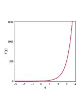
where . It is clear that acts perfectly as cosmological constant DE (DE) with EoS . A generic potential of this type can be obtained by adding a constant to exponential potential (power law inflation), see Figure 21(a). We will see later this potential pattern is recommended to perform and modes of the power spectrum polarization. The first term in (44) is the vacuum energy density (cosmological constant) of the false vacuum spacetime, while the second term associated to the vacuum potential represents a phase transition potential dragging the universe away from false vacuum ( state) to a true vacuum ( state) at its minimum effective potential. However, the EoS still during the whole stage. Now, we investigate the phase transition potential in (44). Using the relation (39) we write the potential in terms the canonical scalar field as
which gives an inverse square law potential. This type of potentials represents the original class of quintessence fields. Indeed, the later expression shows a minimum effective potential only at or with a potential barrier at , while (44) allows the full range . But as the inflation occurs only in a single plateau, then the two expression are identical at .
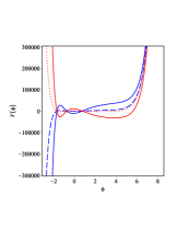
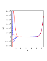
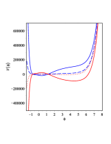
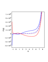
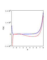
5.4.2 The -model
We take the expansions up to the first order giving the triple
| (45) | |||||
| (46) | |||||
| (47) |
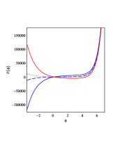
The which is usually used to identify the CDM. In this model, the additional terms of the potential , given by (47), contribute to decrease the potential relative to the kinetic energy. This allows the EoS to evolve above the DE value by , i.e. , which is in agreement with the previous results of Subsection 4.2. Moreover, the potential reduces to where . However, the nonvanishing values of show interesting patterns, there plots appear in Figure 21(b), they predict similar behaviours at where the potentials are nearly flat at the false vacuum () slowly rolls to its effective minimum at the true vacuum (). At , the potentials predict different behaviours according to the value of . At very small negative or positive values of the potentials are nearly flat. The large positive produces Starobinsky-like model where the potential blows up exponentially. Nevertheless, the large negative turns the potential to a quadratic-like model.
5.4.3 The -model
With higher order expansion we have these triple
| (48) | |||||
| (49) | |||||
| (50) | |||||
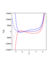
This case still in the quintessence range where . The potential reduces to at the limit where the kinetic dominates over the potential. On the other hand, reduces to the original Starobinsky potential where kinetic energy is negligible during the inflation. The Starobinsky pattern is clear in Figure 21(c) in the case where the potential is dominant. The non-vanishing values of produce almost the same behaviour at , while they produce different behaviours at . In contrast to the , the large negative allows Starobinsky-like model to dominate the epoch while the large positive turns the potential to a quadratic-like model, see Figure 21(c), at . Its plot shows two different minima allowing inflation in both .
5.4.4 The -model
We study one more case where the triple are given by
| (51) | |||||
| (52) | |||||
The evolution of the EoS for this case has been studied in this work in Subsection 4.2. The interest in this case is motivated by the study of the so-called “tracker field" when assuming the inflation ends at ZWS98 . The potential reduces to when vanishes, its nonvanshing values show general behaviours similar to . Whereas, Figure 21(d) shows that, in particular for large negative , the false vacuum is separated by a broad barrier. However, the top of the barrier is quite flat. The decay of the false vacuum is followed by slow-roll inflation allowing a tunneling event from the high energy false vacuum. We find this model fulfills the requirements of BHS13 to perform well fitting both -mode and -mode polarizations.
5.4.5 The -models
For the -model we find it similar to -model but with strong flat plateau at of the false vacuum. At the symmetry of negative and positive large values of no longer valid, see plots of Figure 21(e). The -models, the symmetry of large holds again but they alter their roles, see plots of Figure 21(f)-1(h). Moreover, the asymptotic EoS goes to increase by with a radiation limit for while gives stiff matter, all higher order expansions give unknown matter, so far, with . In order to check the consistency of the results which are obtained by the gravity and by the scalar field of the FRW model, we use equations (36)-(41) to evaluate the dynamical EoS of the scalar field, , according to the order of expansion. The calculations show that the EoS of the model predict a cosmological constant like DE . While the additional terms of the series of in (41) diminishes the effective potential gradually allowing the kinetic energy to showup effectively as the order of expansion increases so that the EoS approaches different asymptotic values with arithmetic sequence respectively. So the rushing of the EoS towards is powered by the kinetic energy of the scalar field. When the higher orders of expansion of (41) are taken into consideration, the kinetic energy is enough to end the cosmic inflation allowing the EoS to crossover to enter a matter dominant universe epoch. It is clear that the scalar field analysis is in agreement with the results of the treatment in Subsection 4.2.
Now back to the plots of Figure 2, the overall picture shows similar behaviours for all the models at while they interpolate between Starobinsky and polynomial potentials at with different details as mentioned above. It is known that the -mode polarization excludes the small tensor-to-scalar ratio models such as Starobinsky model BICEP2 . In contrast, the Planck data restricts the tensor-to-scalar ratio to be small so it excludes inflationary models such as large-field inflation models with a single monomial term Pl1 ; Pl2 . In this theory, we find that the inflationary potential interpolates between these two different classes of inflation. These results lead us to investigate the inflationary parameters within this theory.
6 Single-scalar Field with Double Slowly-rolling Solutions
Assuming that the inflation epoch is dominated by the scalar field potential only. The slow-roll models define two parameters as
| (54) |
These parameters are called slow-roll parameters. Consequently, the slow-roll inflation is valid where and when the potential is dominating. While the end of inflation is characterized by as the kinetic term contribution becomes more effective. The slow-roll parameters define two observable parameters
| (55) |
where and are called the tensor-to-scalar ratio and scalar tilt, respectively. Recent observations by Planck and BICEP2 measure almost the same scalar tilt parameters . However, Planck puts an upper limit which supports models with small . While BICEP2 sets a lower limit on the which supports inflationary models with large . We devote this Section to investigate the capability of the slow-roll models to perform both Planck and BICEP2.
6.1 Construct a potential from Planck and BICEP2
It is clear that Planck and BICEP2 observations agree on the scalar tilt parameter value , while they give different tensor-to-scalar ratios . In order to construct a scalar potential performing Planck and BICEP2 data, we found that if the slow-roll parameters (54) satisfy the proportionality relation , this gives a chance to find two values of performing the same but two different values of . Consequently, two values of . This can be achieved as follows: using (55) and the proportionality relation we have
| (56) |
where is a constant coefficient and are due to the discriminant. It is clear that there are possibly two different values of the parameter for a single scalar tilt parameter . Accordingly, we have which provides double values of for each . More concretely, assuming the scalar tilt parameter Pl2 and substituting into (6.1), for a particular choice of the constant ; then we calculate two possible values of as
-
(i)
The first solution has a positive value of which gives .
-
(ii)
The second solution of has a negative value of which leads to .
Surely both positive and negative values of give the same scalar tilt . Nevertheless, we can get two simultaneous tensor-to-scalar ratios: the first is , while the other is smaller . We conclude that the slow-roll inflationary models which are characterized by the proportionality can perform both -mode and -mode polarizations BHS13 , when a negative value of is observed near the peak of , it would need to be offset by a positive value of at some later time over a comparable field range in order to get to be small again during the period of observable inflation. Generally, at low values of the model predicts one small value of in addition to another higher value as required by the -mode polarization inflationary models. Interestingly, at large values of the model predicts a single value of the tensor-to-scalar parameter which agrees with the upper Plank limit at CL.
Moreover, we can investigate the potential pattern which is characterized by the proportionality relation . Recalling (54), this relation provides a simple differential equation with a solution
| (57) |
where and are constants of integration. In this way, we found that Starobinsky model might be reconstructed naturally from observations if we want our model to perform -mode and -mode polarizations.
6.2 The slow-roll parameters of the model
We calculate the slow roll parameters of the -model to investigate its capability to predict a vaiable inflation. It can be shown that the potential (44) coincides with the potential constructed from Plank and BICEP2 observations (57). Using (44) and (54), we evaluate the slow-roll parameters
| (58) | |||||
| (59) |
From the slow-roll parameters (58) and (59) of the -model, it can be shown that the model satisfies the proportionality , where the proportionality constant . This relation is not only independent of the values of but also it allows a vanishing cosmological constant to exist without affecting the generality of the proportionality relation. Similar relation has been obtained in the literature when studying the leading term behaviour of the Starobinsky inflation as a special case of the -models CGP14 . The number -folds from the end of inflation to the time of horizon crossing for observable scales
| (60) | |||||
where is the value of at the end of inflation. Using (58)-(60) we can reexpress the slow-roll parameters as functions of . At the end of inflation, i.e. Max(, )=1, for the allowed range of the observable cosmological wavelengths exit the Hubble radius for a minimum and maximum inflationary scale we have . In the following steps we show the capability of the models to predict two tensor-to-scalar ratios for a single spectral tilt at different -folds. Using (60) we evaluate the spectral scalar tilt of the -model as a function of . Substituting into (56) we evaluate two values and , for each we have two possible values and , respectively. Finally, we have two tensor-to-scalar ratios , while the two expected spectral scalar tilt are identical, i.e. . This procedure enables to draw the plots of Figure 3. The plots represent the evolution of the observable parameters vs the -folding number. As is clear the spectral scalar tilt has a single pattern represented by plot, while the tensor-to-scalar ratio has two distinguished patterns represented by and plots. The has a lower limit which is in agreement with the -mode polarization models. On the other hand, the plot has an upper limit which is in agreement with the -mode polarization models.
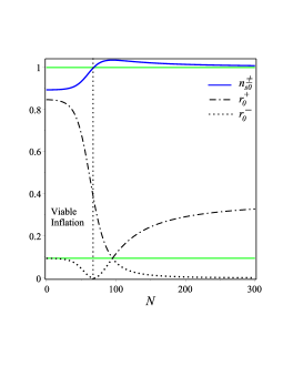
In Figure 3, the viable inflation is characterized by region. The region with exceeding unity is Max, although this small deviation from the scale invariance of the scalar power spectrum is acceptable at the level of theoretical predictions, it can be excluded as it appears beyond the acceptable range of the -folds . Interestingly, at large -folding number the spectral scalar tilt goes again below unity so that . We highlight some results in Table 1 showing that the -model can predict large tensor-to-scalar ratios of the -mode polarization as well as small ratios as required by the -mode polarization.
Similar procedure can be applied to the -model where the relation still valid with larger proportionality constant . Accordingly, the tensor-to-scalar ratios can be achieved, e.g. at we have (, , ) = (, , ) where the scalar tilt in this case always . Also, this procedure can be used to put constraints on the choice of conformal weight in the power law and Starobinsky inflation models from the CMB observations444This work is in progress now..
7 Discussions and Final Remarks
We investigate a special class of gravity governed by FLU assumptions. In this model, we assume the vanishing of the coefficient of the sectional curvature in the modified Friedmann equations. This enables to identify a particular class of gravity, usually hidden by the SFU assumption, cannot be covered by TEGR theory. The FLU model, at large Hubble regime, is consistent with the cosmic inflation scenario. Also, it enables to evaluate a dynamical EoS of the cosmic fluid. In a particular case , the fluid can evolve from phantom initial phase crossing the phantom divided line () to radiation and possibly stiff-matter with a quintessence fate. As a matter of fact, the dynamical EoS avoids the usual problems of the cosmological constant DE models. In addition, there is no need to assume a large cosmological constant at early universe.
We provide an alternative approach to study inflation by considering the case when the torsion is made of a scalar field . This approach allows the to predict the inflationary observable parameters. We show that the teleparallel torsion scalar can couple to the kinetic energy of the scalar field, while its potential can be induced by the gravity. In this case, we define a scalar field sensitive to the spacetime symmetry with a potential induced exactly from extended teleparallel gravity. This leads finally to a gravitational quintessence model governed by Friedmann and Klein-Gordon equations.
The obtained quintessence model covers different inflationary models according to the expansion limit. In this study, we give more attention to the -model. It has been shown that the model relates the slow-roll parameters by the proportionality which in agreement with the model constructed from Planck and BICEP2 data. The model can be classified as power law inflation which has been shown that is capable of performing two tensor-to-scalar ratios consistent with both and modes of polarization, while it predicted scalar spectral index still unique. In particular, the observable parameters evolution with the -folding can be shown in Figure 3 and Table 1. We just highlighted some results of the other models, while further studies are left for future work. Higher orders potentials interpolate between Starobinsky and quadratic like inflations.
Finally, we would like to mention that at large the model predicts a single tensor-to-scalar parameter in agreement with Planck observations limit. This result can be used to constrain the choice of the conformal weight in power law and Starobinsky models to the observable parameters of the cosmic inflation epoch.
Acknowledgments
The authors would like to thank the anonymous Referee for her/his valuable comments which, indeed, help to improve the work. This article is partially supported by the Egyptian Ministry of Scientific Research under project No. 24-2-12.
References
- (1) A. G. Riess, A. V. Filippenko, P. C. et. al., Astrophys. J. 116, 1009 (1998), astro-ph/9805201
- (2) R. Aldrovandi, J. G. Pereira, Teleparallel Gravity: An Introduction, vol. 173 of Fundamental Theories of Physics (Springer, Springer Dordrecht Heidelberg New York London, 2013)
- (3) B. Li, T. P. Sotiriou, J. D. Barrow, Phys. Rev. D 83, 6, 064035 (2011), 1010.1041
- (4) T. P. Sotiriou, B. Li, J. D. Barrow, Phys. Rev. D 83, 10, 104030 (2011), 1012.4039
- (5) A. Einstein, Riemann-Geometrie mit Aufrechterhaltung des Begriffes des Fernparallelismus, 217 – 221, Phys.-math. Klasse (Preussische Akademie der Wissenschaften, Sitzungsberichte, 1928)
- (6) F. I. Mikhail, Relativistic cosmology and some related problems in general relativity, Ph. D. Thesis, University of London (1952)
- (7) W. H. McCrea, F. I. Mikhail, Royal Society of London Proceedings Series A 235, 11 (1956)
- (8) F. Mikhail, Al Nuovo Cimento series X, 32, 886 (1964)
- (9) F. I. Mikhail, M. I. Wanas, Royal Society of London Proceedings Series A 356, 471 (1977)
- (10) C. Møller, K. Dan. Vidensk. Selsk. Mat. Fys. Skr. 89, 13 (1978)
- (11) K. Hayashi, T. Shirafuji, Phys. Rev. D 19, 3524 (1979)
- (12) R. Utiyama, Physical Rev. 101, 5, 1597 (1956)
- (13) T. W. B. Kibble, J. Math. Phys. 2, 2, 212 (1961)
- (14) D. W. Sciama, Rev. Mod. Phys. 463–469 (1964)
- (15) F. W. Hehl, P. von der Heyde, G. D. Kerlick, et al., Reviews of Modern Physics 48, 393 (1976)
- (16) R. Utiyama, Progress of Theoretical Physics 64, 2207 (1980)
- (17) N. L. Youssef, A. M. Sid-Ahmed, Reports on Mathematical Physics 60, 39 (2007), 0604111
- (18) N. L. Youssef, W. A. Elsayed, Reports on Mathematical Physics 72, 1 (2013), 1209.1379
- (19) M. I. Wanas, Modern Physics Letters A 24, 1749 (2009), %****␣1409.7199.bbl␣Line␣75␣****0801.1132
- (20) M. I. Wanas, M. M. Kamal, Modern Physics Letters A 26, 2065 (2011), 1103.4121
- (21) N. L. Youssef, A. M. Sid-Ahmed, E. H. Taha, Int. J. Geom. Meth. Mod. Phys. 10, 7, 1350029 (2013), 1206.4505
- (22) R. Ferraro, F. Fiorini, Phys. Rev. D 75, 8, 084031 (2007), gr-qc/0610067
- (23) R. Ferraro, F. Fiorini, Phys. Rev. D 78, 12, 124019 (2008), gr-qc/0812.1981
- (24) G. R. Bengochea, R. Ferraro, Phys. Rev. D 79, 12, 124019 (2009), 0812.1205
- (25) E. V. Linder, Phys. Rev. D 81, 12, 127301 (2010), 1005.3039
- (26) K. Bamba, C.-Q. Geng, C.-C. Lee, ArXiv e-prints (2010), 1008.4036
- (27) K. Bamba, C.-Q. Geng, C.-C. Lee, et al., JCAP 1, 021 (2011), 1011.0508
- (28) R.-J. Yang, EPL (Europhysics Letters) 93, 60001 (2011), 1010.1376
- (29) S.-H. Chen, J. B. Dent, S. Dutta, et al., Phys. Rev. D 83, 2, 023508 (2011), 1008.1250
- (30) R. Ferraro, F. Fiorini, Phys. Rev. D 84, 8, 083518 (2011), 1109.4209
- (31) R. Ferraro, F. Fiorini, Phys. Lett. B 702, 75 (2011), 1103.0824
- (32) L. Iorio, E. N. Saridakis, Mon. Not. R. Astron. Soc. 427, 1555 (2012), 1203.5781
- (33) S. Capozziello, P. A. González, E. N. Saridakis, et al., JHEP 2, 39 (2013), 1210.1098
- (34) G. G. L. Nashed, Phys. Rev. D 88, 10, 104034 (2013), 1311.3131
- (35) G. G. L. Nashed, General Relativity and Gravitation 45, 1887 (2013), 1502.05219
- (36) M. E. Rodrigues, M. J. S. Houndjo, J. Tossa, et al., JCAP 11, 024 (2013), 1306.2280
- (37) G. G. L. Nashed, EPL (Europhysics Letters) 105, 10001 (2014), 1501.00974
- (38) C. Bejarano, R. Ferraro, M. J. Guzmán, Eur. Phys. J. C 75, 77 (2015), 1412.0641
- (39) G. G. L. Nashed, Journal of the Physical Society of Japan 84, 4, 044006 (2015)
- (40) G. G. L. Nashed, International Journal of Modern Physics D 24, 1550007 (2015)
- (41) K. Bamba, S. Capozziello, S. Nojiri, et al., Astrophysics and Space Science 342, 155 (2012), 1205.3421
- (42) K. Bamba, S. Nojiri, S. D. Odintsov, Phys. Lett. 257–264 (2014), 1401.7378
- (43) K. Bamba, S. D. Odintsov, ArXiv: 1402.7114 (2014), 1402.7114
- (44) M. Jamil, D. Momeni, R. Myrzakulov, International Journal of Theoretical Physics (2014), 1309.3269
- (45) T. Harko, F. S. N. Lobo, G. Otalora, et al., Phys. Rev. D 89, 12, 124036 (2014), 1404.6212
- (46) G. G. L. Nashed, W. El Hanafy, European Physical Journal C 74, 10, 3099 (2014), arXiv: 1403.0913, 1403.0913
- (47) M. I. Wanas, H. A. Hassan, International Journal of Theoretical Physics 53, 3901 (2014)
- (48) W. El Hanafy, G. G. L. Nashed (2014), 1410.2467
- (49) Y. Wu, Z.-C. Chen, J. Wang, et al., ArXiv e-prints (2015), 1503.05281
- (50) E. L. B. Junior, M. E. Rodrigues, M. J. S. Houndjo, ArXiv e-prints (2015), 1503.07427
- (51) Y.-F. Cai, S.-H. Chen, J. B. Dent, et al., Classical and Quantum Gravity 28, 21, 215011 (2011), 1104.4349
- (52) Y.-F. Cai, J. Quintin, E. N. Saridakis, et al., JCAP 7, 033 (2014), 1404.4364
- (53) G. Nashed, W. El Hanafy, S. Ibrahim (2014), 1411.3293
- (54) G. Kofinas, E. N. Saridakis, Phys. Rev. D 90, 8, 084044 (2014), 1404.2249
- (55) G. Kofinas, E. N. Saridakis, Phys. Rev. D 90, 8, 084045 (2014), 1408.0107
- (56) G. Kofinas, G. Leon, E. N. Saridakis, Classical and Quantum Gravity 31, 17, 175011 (2014), 1404.7100
- (57) Planck Collaboration, P. A. R. Ade, N. Aghanim, et al., Astronomy & Astrophysics 571 (2014), 1303.5082
- (58) Planck Collaboration, P. A. R. Ade, N. Aghanim, et al., Astronomy & Astrophysics 571 (2014), 1303.5076
- (59) BICEP2 Collaboration, P. A. R. Ade, et al., Physical Review Letters 112, 24, 241101 (2014), 1403.3985
- (60) J. W. Maluf, Annalen der Physik 525, 339 (2013), 1303.3897
- (61) H. P. Robertson, Ann. Math. 33, 496 (1932)
- (62) O. Farooq, D. Mania, B. Ratra, Astrophysics and Space Science 357, 11 (2015)
- (63) J. N. Dossett, M. Ishak, Phys. Rev. D 86, 10, 103008 (2012), 1205.2422
- (64) J.-F. Zhang, M.-M. Zhao, J.-L. Cui, et al., European Physical Journal C 74, 3178 (2014), 1409.6078
- (65) V. Sahni, Classical and Quantum Gravity 19, 3435 (2002), astro-ph/0202076
- (66) M. I. Wanas, Adv. High Energy Phys. 2012, Article ID 752613, 10 pages (2012)
- (67) H.-j. Xie, T. Shirafuji (1996), 9603006
- (68) V. E. Rochev, Theoretical and Mathematical Physics 18, 160 (1974)
- (69) S. Hojman, M. Rosenbaum, M. P. Ryan, et al., Phys. Rev. D 17, 3141 (1978)
- (70) R. T. Hammond, Classical and Quantum Gravity 7, 2107 (1990)
- (71) F. W. Hehl, Y. N. Obukhov, in C. Lämmerzahl, C. W. F. Everitt, F. W. Hehl, eds., Gyros, Clocks, Interferometers …: Testing Relativistic Gravity in Space, vol. 562 of Lecture Notes in Physics, Berlin Springer Verlag, 479 (2001), gr-qc/0001010
- (72) V. C. de Andrade, J. G. Pereira, General Relativity and Gravitation 30, 263 (1998), 9706070
- (73) A. Einstein, The meaning of relativity, 5th edn. (the Princeton University Press, 1955)
- (74) J. B. Fonseca-Neto, C. Romero, S. P. G. Martinez, General Relativity and Gravitation 45, 1579 (2013), 1211.1557
- (75) L. Y. Nabil, A. M. Sid-Ahmed, in M. Wanas, ed., The international conference on developing and extending Einstein’s ideas, 19–21, Egyptian Relativity Group (NART, Cairo, Egypt, 2005)
- (76) R. Kallosh, A. Linde, D. Roest, JHEP 8, 52 (2014), 1405.3646
- (77) A. A. Starobinsky, Phys. Lett. B 91, 99 (1980)
- (78) I. Zlatev, L. Wang, P. J. Steinhardt, Physical Review Letters 82, 896 (1999), astro-ph/9807002
- (79) R. Bousso, D. Harlow, L. Senatore, Phys.Rev. D 91, 8, 083527 (2015), 1309.4060
- (80) Y.-F. Cai, J.-O. Gong, S. Pi, Phys. Lett. B 738, 20 (2014), 1404.2560