Nonminimal torsion-matter coupling extension of $f(T)$ gravity

Abstract

We construct an extension of $f(T)$ gravity with the inclusion of a non-minimal torsion-matter coupling in the action. The resulting theory is a novel gravitational modification, since it is different from both $f(T)$ gravity, as well as from the nonminimal curvature-matter-coupled theory. The cosmological application of this new theory proves to be very interesting. In particular, we obtain an effective dark energy sector whose equation-of-state parameter can be quintessence- or phantom-like, or exhibit the phantom-divide crossing, while for a large range of the model parameters the universe results in a de Sitter, dark-energy-dominated, accelerating phase. Additionally, we can obtain early-time inflationary solutions too, and thus provide a unified description of the cosmological history.

I Introduction

The recent observational advances in cosmology have provided a large amount of high-precision cosmological data, which has posed new challenges for the understanding of the basic physical properties of the Universe, and of the gravitational interaction that dominates its dynamics and evolution. The observation of the accelerated expansion of the Universe Riess1 has raised the fundamental issue of the cause of this acceleration, which is usually attributed to a mysterious and yet not directly detected dominant component of the Universe, called dark energy Copeland:2006wr . In this context, the recently released Planck satellite data of the 2.7 degree Cosmic Microwave Background (CMB) full sky survey Planckresults have generally confirmed the standard $\Lambda$ Cold Dark Matter ($\Lambda$CDM) cosmological model. On the other hand, the measurement of the tensor modes from large angle CMB B-mode polarisation by BICEP2 BICEP2 , implying a tensor-to-scalar ratio $r=0.2^{+0.07}_{-0.05}$, has provided a very convincing evidence for the inflationary scenario, since the generation of gravitational wave fluctuations is a generic prediction of the early de Sitter exponential expansion. However, the BICEP2 result is in tension with Planck limits on standard inflationary models Mar , and thus alternative explanations may be required. In principle, magnetic fields generated during inflation can produce the required B-mode, for a suitable range of energy scales of inflation Mar . Moreover, the existence of the fluctuations of cosmological birefringence can give rise to CMB B-mode polarization that fits BICEP2 data with $r<0.11$, and no running of the scalar spectral index Lee .

The above major observational advances require some good theoretical explanations, with the role of giving a firm foundation to cosmology, and the underlying theory of gravity. However, up to now, no convincing theoretical model, supported by observational evidence that could clearly explain the nature of dark energy, has been proposed. Moreover, not only the recent accelerated expansion of the Universe, but also observations at the galactic (galaxy rotation curves) and extra-galactic scale (virial mass discrepancy in galaxy clusters) Str suggest the existence of another mysterious and yet undetected major component of the Universe, the so-called dark matter. From all these observations one can conclude that the standard general relativistic gravitational field equations, obtained from the classic Einstein-Hilbert action $S=\int{\left(R/2+L_{m}\right)\sqrt{-g}d^{4}x}$, where $R$ is the scalar curvature, and $L_{m}$ is the matter Lagrangian density, in which matter is minimally coupled to the geometry, cannot give an appropriate quantitative description of the Universe at astrophysical scales going beyond the boundary of the Solar System. To explain dark energy and dark matter in a cosmological context requires the ad hoc introduction of the dark matter and dark energy components into the total energy-momentum tensor of the Universe, in addition to the ordinary baryonic matter.

From a historical point of view, in going beyond the Einstein-Hilbert action, the first steps were taken in the direction of generalizing the geometric part of the standard gravitational action. An extension of the Einstein-Hilbert action, in which the Ricci scalar invariant $R$ is substituted with an arbitrary function of the scalar invariant, $f(R)$, has been extensively explored in the literature rev . Such a modification of the gravitational action can explain the late acceleration of the Universe, and may also provide a geometric explanation for dark matter, which can be described as a manifestation of geometry itself Boehm . Furthermore, quadratic Lagrangians, constructed from second order curvature invariants such as $R^{2}$, $R_{\mu\nu}R^{\mu\nu}$, $R_{\alpha\beta\mu\nu}R^{\alpha\beta\mu\nu}$, $\varepsilon^{\alpha\beta\mu\nu}R_{\alpha\beta\gamma\delta}R_{\mu\nu}^{\gamma\delta}$, $C_{\alpha\beta\mu\nu}C^{\alpha\beta\mu\nu}$, etc., have also been considered as candidates for a more general gravitational actions Lobo:2008sg , which can successfully explain dark matter and the late-time cosmic acceleration. Alternatively, the interest for extra-dimensions, which goes back to the unified field theory of Kaluza and Klein, led to the development of the braneworld models Maartens1 . In braneworld models, gravitational effects due to the extra dimensions dominate at high energies, but important new effects, which can successfully explain both dark energy and dark matter, also appear at low energies.

Most of the modifications of the Einstein-Hilbert Lagrangian involve a change in the geometric part of the action only, and assume that the matter Lagrangian plays a subordinate and passive role, which is implemented by the minimal coupling of matter to geometry. However, a general theoretical principle forbidding an arbitrary coupling between matter and geometry does not exist a priori. If theoretical models, in which matter is considered on an equal footing with geometry, are allowed, gravitational theories with many interesting and novel features can be constructed.

A theory with an explicit coupling between an arbitrary function of the scalar curvature and the Lagrangian density of matter was proposed in Bertolami:2007gv . The gravitational action of the latter model is of the form $S=\int{\left\{f_{1}(R)+\left[1+\lambda f_{2}(R)\right]L_{m}\right\}\sqrt{-g}d^{4}x}$. In these models an extra force acting on massive test particles arises, and the motion is no longer geodesic. Moreover, in this framework, one can also explain dark matter Bertolami:2009ic . The early “linear” geometry-matter coupling Bertolami:2007gv was extended in Harko:2008qz and a maximal extension of the Einstein-Hilbert action with geometry-matter coupling, of the form $S=\int d^{4}x\sqrt{-g}f\left(R,L_{m}\right)$ was considered in Harko:2010mv . An alternative model to $f(R,L_{m})$ gravity is the $f(R,\mathcal{T})$ theory Harko:2011kv , where $\mathcal{T}$ is the trace of the matter energy-momentum tensor $T_{\mu\nu}$, and the corresponding action given by $S=\int{\left[f\left(R,\mathcal{T}\right)/2+L_{m}\right]\sqrt{-g}d^{4}x}$. The dependence of the gravitational action on $\mathcal{T}$ may be due to the presence of quantum effects (conformal anomaly), or of some exotic imperfect fluids. When the trace of the energy-momentum tensor $\mathcal{T}$ is zero, $\mathcal{T}=0$, which is the case for the electromagnetic radiation, the field equations of $f(R,T)$ theory reduce to those of $f(R)$ gravity.

However, the $f(R,L_{m})$ or $f(R,\mathcal{T})$ gravitational models are not the most general Lagrangians with nonminimal geometry-matter couplings. One could further obtain interesting gravity models by introducing a term of the form $R_{\mu\nu}T^{\mu\nu}$ into the Lagrangian fRT ; Od . Such couplings appear in Einstein-Born-Infeld theories deser , when one expands the square root in the Lagrangian. The presence of the $R_{\mu\nu}T^{\mu\nu}$ coupling term has the advantage of entailing a nonminimal coupling of geometry to the electromagnetic field.

All the above gravitational modifications are based on the Einstein-Hilbert action, namely on the curvature description of gravity. However, an interesting and rich class of modified gravity can arise if one modifies the action of the equivalent torsional formulation of General Relativity. As it is well known, Einstein also constructed the “Teleparallel Equivalent of General Relativity” (TEGR) Unzicker:2005in ; TEGR ; Hayashi:1979qx ; JGPereira ; Maluf:2013gaa , replacing the torsion-less Levi-Civita connection by the curvature-less Weitzenböck one, and using the vierbein instead of the metric as the fundamental field. In this formulation, instead of the curvature (Riemann) tensor one has the torsion tensor, and the Lagrangian of the theory, namely the torsion scalar $T$, is constructed by contractions of the torsion tensor. Thus, if one desires to modify gravity in this formulation, the simplest thing is to extend $T$ to an arbitrary function$f(T)$ Ferraro:2006jd ; Linder:2010py . An interesting aspect of this extension is that although TEGR coincides with General Relativity at the level of equations, $f(T)$ is different than $f(R)$, that is they belong to different modification classes. Additionally, although in $f(R)$ theory the field equations are fourth order, in $f(T)$ gravity they are second order, which is a great advantage. $f(T)$ gravity models have been extensively applied to cosmology, and amongst other applications it is able to explain the late-time accelerating expansion of the Universe without the need for dark energy Linder:2010py ; Chen:2010va ; Bengochea001 . Furthermore, following these lines, and inspired by the higher-curvature modifications of General Relativity, one can construct gravitational modifications based on higher-order torsion invariants, such is the $f(T,T_{G})$ gravity Kofinas:2014owa , which also proves to have interesting cosmological implications.

Another gravitational modification based on the teleparallel formulation is the generalization of TEGR to the case of a Weyl-Cartan space-time, in which the Weitzenböck condition of the vanishing of the curvature is also imposed (Weyl-Cartan-Weitzenböck (WCW) gravity), with the addition of a kinetic term for the torsion in the gravitational action WC1 . In this framework the late-time acceleration of the Universe can be naturally obtained, determined by the intrinsic geometry of the space-time. A further extension of the WCW gravity, in which the Weitzenböck condition in a Weyl-Cartan geometry is inserted into the gravitational action via a Lagrange multiplier, was analyzed in WC2 . In the weak field limit the gravitational potential explicitly depends on the Lagrange multiplier and on the Weyl vector, leading to an interesting cosmological behavior.

In the work, we are interested in proposing a novel gravitational modification based on the torsional formulation, by allowing the possibility of a nonminimal torsion-matter coupling in the gravitational action. In particular, for the torsion-matter coupling we adopt the “linear” model introduced in the case of $f(R)$ gravity in Bertolami:2007gv . Hence, the gravitational field can be described in terms of two arbitrary functions of the torsion scalar $T$, namely $f_{1}(T)$ and $f_{2}(T)$, with the function $f_{2}(T)$ linearly coupled to the matter Lagrangian. This new coupling induces a supplementary term $\left[1+\lambda f_{2}(T)\right]L_{m}$ in the standard $f(T)$ action, with $\lambda$ an arbitrary coupling constant. When $\lambda=0$, the model reduces to the usual $f(T)$ gravity. We investigate in detail the cosmological implications of the torsion-matter coupling for two particular choices of the functions $f_{1}(T)$ and $f_{2}(T)$. For both choices the Universe evolution is in agreement with the observed behavior, and moreover it ends in a de Sitter type vacuum state, with zero matter energy density. The details of the transition depend on the numerical values of the free parameters that appear in the functions $f_{1}(T)$ and $f_{2}(T)$.

The paper is organized as follows. In Section II we briefly describe the basics of the $f(T)$ gravity model. The field equations of the $f(T)$ theory with linear nonminimal torsion-matter coupling are obtained in Section III. The cosmological implications of the theory are analyzed in Section IV. Finally, we conclude and discuss our results in Section V.

II $f(T)$ gravity and Cosmology

In this Section, we briefly review the $f(T)$ gravitational paradigm. We use the notation where Greek indices run over the coordinate space-time and Latin indices run over the tangent space-time. As we mentioned in the Introduction, the dynamical variables are the vierbein fields ${\mathbf{e}_{A}(x^{\mu})}$, which at each point $x^{\mu}$ of the manifold form an orthonormal basis for the tangent space, that is $\mathbf{e}_{A}\cdot\mathbf{e}_{B}=\eta_{AB}$, with $\eta_{AB}={\rm diag}(1,-1,-1,-1)$. Additionally, they can be expressed in terms of the components $e_{A}^{\mu}$ in the coordinate basis as $\mathbf{e}_{A}=e^{\mu}_{A}\partial_{\mu}$. Hence, the metric is obtained from the dual vierbein through

$$g_{\mu\nu}(x)=\eta_{AB}\,e^{A}_{\mu}(x)\,e^{B}_{\nu}(x).$$ (1)

In this formulation, instead of the Levi-Civita connection one uses the Weitzenböck one: $\overset{\mathbf{w}}{\Gamma}^{\lambda}_{\nu\mu}\equiv e^{\lambda}_{A}\>\partial_{\mu}e^{A}_{\nu}$ Weitzenb23 , and thus instead of curvature we acquire the torsion tensor

$${T}^{\lambda}_{\>\mu\nu}=\overset{\mathbf{w}}{\Gamma}^{\lambda}_{\nu\mu}-\overset{\mathbf{w}}{\Gamma}^{\lambda}_{\mu\nu}=e^{\lambda}_{A}\>(\partial_{\mu}e^{A}_{\nu}-\partial_{\nu}e^{A}_{\mu}).$$ (2)

It proves convenient to define the contorsion tensor $K^{\mu\nu}{}_{\rho}\equiv-\frac{1}{2}\Big{(}T^{\mu\nu}{}_{\rho}-T^{\nu\mu}{}_{\rho}-T_{\rho}{}^{\mu\nu}\Big{)}$, as well as the tensor $S_{\rho}{}^{\mu\nu}\equiv\frac{1}{2}\Big{(}K^{\mu\nu}{}_{\rho}+\delta^{\mu}_{\rho}\>T^{\alpha\nu}{}_{\alpha}-\delta^{\nu}_{\rho}\>T^{\alpha\mu}{}_{\alpha}\Big{)}$. Using these one can write down the teleparallel Lagrangian (torsion scalar) TEGR ; Hayashi:1979qx ; JGPereira ; Maluf:2013gaa ; Maluf:1994ji

$$T\equiv\frac{1}{4}T^{\rho\mu\nu}T_{\rho\mu\nu}+\frac{1}{2}T^{\rho\mu\nu}T_{\nu\mu\rho}-T_{\rho\mu}{}^{\rho}T^{\nu\mu}{}_{\nu},$$ (3)

which used in the action and varied in terms of the vierbeins gives rise to the same equations with General Relativity. That is why such a theory is called “Teleparallel Equivalent of General Relativity” (TEGR).

One can be based on the above torsional formulation of General Relativity, in order to construct classes of modified gravity. The simplest one is to extend $T$ to a function $T+f(T)$, that is writing an action of the form

$$S=\frac{1}{16\pi G}\int d^{4}xe\left[T+f(T)\right],$$ (4)

where $e=\text{det}(e_{\mu}^{A})=\sqrt{-g}$, $G$ is the gravitational constant, and we have used units where the speed of light is $c=1$. Note that TEGR and thus General Relativity is restored when $f(T)=0$. Moreover, we stress that although TEGR coincides with General Relativity at the level of equations, $f(T)$ is different than $f(R)$.

Let us now proceed to the cosmological application of $f(T)$ gravity. Introducing additionally the matter sector the total action becomes

$$S=\frac{1}{16\pi G}\int d^{4}xe\left[T+f(T)+L_{m}\right],$$ (5)

where the matter Lagrangian is assumed to correspond to a perfect fluid with energy density $\rho_{m}$ and pressure $p_{m}$ (for simplicity we neglect the radiation sector, although its inclusion is straightforward). Varying the action (5) with respect to the vierbeins we obtain the field equations

$$\left(1+f^{\prime}\right)\,\left[e^{-1}\partial_{\mu}(ee_{A}^{\rho}S_{\rho}{}^{\nu\mu})-e_{A}^{\lambda}T^{\rho}{}_{\mu\lambda}S_{\rho}{}^{\mu\nu}\right]$$

$$+e_{A}^{\rho}S_{\rho}{}^{\nu\mu}\partial_{\mu}{T}f^{\prime\prime}+\frac{1}{4}e_{A}^{\nu}[T+f]=4\pi Ge_{A}^{\rho}\overset{\mathbf{em}}{T}_{\rho}{}^{\nu},$$ (6)

where $f^{\prime}=\partial f/\partial T$, $f^{\prime\prime}=\partial^{2}f/\partial T^{2}$, and $\overset{\mathbf{em}}{T}_{\rho}{}^{\nu}$ denotes the usual energy-momentum tensor.

Proceeding forward, we impose the standard homogeneous and isotropic geometry, that is we consider

$$e_{\mu}^{A}={\rm diag}(1,a(t),a(t),a(t)),$$ (7)

which corresponds to a flat Friedmann-Robertson-Walker (FRW) universe with metric

$$ds^{2}=dt^{2}-a^{2}(t)\,\delta_{ij}dx^{i}dx^{j},$$ (8)

where $a(t)$ is the scale factor.

In summary, inserting the vierbein ansantz (7) into the equations of motion (II) we extract the modified Friedmann equations as

$$H^{2}=\frac{8\pi G}{3}\rho_{m}-\frac{f}{6}-2H^{2}f^{\prime}$$ (9)

$$\dot{H}=-\frac{4\pi G(\rho_{m}+p_{m})}{1+f^{\prime}-12H^{2}f^{\prime\prime}},$$ (10)

with $H\equiv\dot{a}/a$ the Hubble parameter, and dots denoting derivatives with respect to $t$. Note that we have also used the relation

$$T=-6H^{2},$$ (11)

which arises immediately for an FRW geometry using Eq. (3).

III $f(T)$ gravity with nonminimal torsion-matter coupling

Having presented the $f(T)$ modified gravity in the previous section, in this section we extend it, allowing for a nonminimal coupling between the torsion scalar and the matter Lagrangian. In particular, we consider the action

$$S=\frac{1}{16\pi G}\,\int d^{4}x\,e\,\left\{T+f_{1}(T)+\left[1+\lambda\,f_{2}(T)\right]\,L_{m}\right\},$$ (12)

where $f_{i}(T)$ (with $i=1,2$) are arbitrary functions of the torsion scalar $T$ and $\lambda$ is a coupling constant with units of ${\rm mass}^{-2}$. Varying the action with respect to the tetrad $e^{A}_{\rho}$ yields the field equations

$$\left(1+f_{1}^{\prime}+\lambda f_{2}^{\prime}L_{m}\right)\left[e^{-1}\partial_{\mu}{(ee^{\alpha}_{A}S_{\alpha}{}^{\rho\mu})}-e^{\alpha}_{A}T^{\mu}{}_{\nu\alpha}S_{\mu}{}^{\nu\rho}\right]$$

$$\ \ \ \ \ +\left(f_{1}^{\prime\prime}+\lambda f_{2}^{\prime\prime}L_{m}\right)\partial_{\mu}{T}e^{\alpha}_{A}S_{\alpha}{}^{\rho\mu}+e_{A}^{\rho}\left(\frac{f_{1}+T}{4}\right)$$

$$\ \ \ \ \ -\frac{1}{4}\lambda f_{2}^{\prime}\,\partial_{\mu}{T}e^{\alpha}_{A}\overset{\mathbf{em}}{S}_{\alpha}{}^{\rho\mu}+\lambda f_{2}^{\prime}\,e^{\alpha}_{A}S_{\alpha}{}^{\rho\mu}\,\partial_{\mu}{L_{m}}$$

$$\ \ \ \ \ =4\pi G\left(1+\lambda f_{2}\right)e^{\alpha}_{A}\overset{\mathbf{em}}{T}_{\alpha}{}^{\rho},$$ (13)

where we have defined

$$\overset{\mathbf{em}}{S}_{A}{}^{\rho\mu}=\frac{\partial{L_{m}}}{\partial{\partial_{\mu}{e^{A}_{\rho}}}},$$ (14)

and the prime denotes differentiation with respect to the torsion scalar. As expected Eq. (13) reduces to Eq. (II) when $\lambda=0$.

Since the Lagrangian density of a perfect fluid is the energy scalar, representing the energy in a local rest frame for the fluid, a possible “natural choice” for the matter Lagrangian density is $L_{m}/(16\pi G)=-\rho_{m}$ GroenHervik ; BPHL . In this case, we have $\overset{\mathbf{em}}{S}_{A}{}^{\rho\mu}=0$, and also the usual form of the energy momentum tensor for the perfect fluid $\overset{\mathbf{em}}{T}_{\mu\nu}=(\rho_{m}+p_{m})u_{\mu}u_{\nu}-p_{m}g_{\mu\nu}$.

In summary, inserting the flat FRW vierbein choice (7) and the above matter Lagrangian density, into the field equations (13), we obtain the modified Friedmann equations

$$H^{2}=\frac{8\pi G}{3}\left[1+\lambda\left(f_{2}+12H^{2}f_{2}^{\prime}\right)\right]\rho_{m}-\frac{1}{6}\left(f_{1}+12H^{2}f_{1}^{\prime}\right),$$ (15)

$$\dot{H}=-\frac{4\pi G\left(\rho_{m}+p_{m}\right)\left[1+\lambda\left(f_{2}+12H^{2}f_{2}^{\prime}\right)\right]}{1+f_{1}^{\prime}-12H^{2}f_{1}^{\prime\prime}-16\pi G\lambda\rho_{m}\left(f_{2}^{\prime}-12H^{2}f_{2}^{\prime\prime}\right)}.$$ (16)

In the limit $\lambda=0$, $f_{1}(T)\equiv f(T)$, and $f_{2}(T)\equiv 0$, Eqs. (15) and (16) reduce to Eqs. (9) and (10), respectively. The generalized Friedmann equations can be rewritten as

$$3H^{2} = 8\pi G\left(\rho_{DE}+\rho_{m}\right),$$ (17)

$$2\dot{H}+3H^{2} = -8\pi G\left(p_{DE}+p_{m}\right),$$ (18)

where the effective energy density and effective pressure of the dark energy sector are defined as

$$\rho_{DE}:=-\frac{1}{16\pi G}\left(f_{1}+12H^{2}f_{1}^{\prime}\right)+\lambda\rho_{m}\left(f_{2}+12H^{2}f_{2}^{\prime}\right),$$ (19)

$$p_{DE}:=\left(\rho_{m}+p_{m}\right)\times$$

$$\left[\frac{1+\lambda\left(f_{2}+12H^{2}f_{2}^{\prime}\right)}{1+f_{1}^{\prime}-12H^{2}f_{1}^{\prime\prime}-16\pi G\lambda\rho_{m}\left(f_{2}^{\prime}-12H^{2}f_{2}^{\prime\prime}\right)}-1\right]$$

$$+\frac{1}{16\pi G}\left(f_{1}+12H^{2}f_{1}^{\prime}\right)-\lambda\rho_{m}\left(f_{2}+12H^{2}f_{2}^{\prime}\right).$$ (20)

Furthermore, we can define the dark-energy equation-of-state parameter in the standard form

$$w_{DE}:=\frac{p_{DE}}{\rho_{DE}}.$$ (21)

One can easily verify that the above affective dark energy density and pressure satisfy the usual evolution equation

$$\dot{\rho}_{DE}+\dot{\rho}_{m}+3H\left(\rho_{DE}+\rho_{m}+p_{DE}+p_{m}\right)=0.$$ (22)

Finally, we can introduce the deceleration parameter $q$, given by

$$q=\frac{d}{dt}\left(\frac{1}{H}\right)-1,$$ (23)

whose sign indicates the decelerating/accelerating nature of the cosmological expansion. Cosmological models with $q<0$ are accelerating, while those having $q>0$ experience a decelerating evolution.

IV Cosmological implications

Since we have extracted the basic background equations of motion of the $f(T)$ gravity model with a nonminimal matter-torsion coupling, we are now able to investigate its phenomenological implications. Due to the relation (11), for convenience in the following we will change the $T$-dependence to the $H$-dependence in the involved expressions, so that $f_{1}(T)\equiv f_{1}(H)$, and $f_{2}(T)\equiv f_{2}(H)$. For the derivatives of the functions $f_{1}(T)$ and $f_{2}(T)$ we obtain $f_{i}^{\prime}(H)\equiv\left.f_{i}^{\prime}(T)\right|_{T\rightarrow-6H^{2}}$, and $f_{i}^{\prime\prime}(H)\equiv\left.f_{i}^{\prime\prime}(T)\right|_{T\rightarrow-6H^{2}}$, $i=1,2$, respectively. Finally, in the following we fully adopt the natural system of units by taking $8\pi G=c=1$.

The basic cosmological equations describing the time evolution of the nonminimally-coupled $f(T)$ gravity are given by Eqs. (15) and (16). From Eq. (15) we can express the matter density as

$$\rho_{m}(t)=\frac{3H^{2}+\left[f_{1}(H)+12H^{2}\left.f_{1}^{\prime}(T)\right|_{T\rightarrow-6H^{2}}\right]/2}{1+\lambda\left[f_{2}(H)+12H^{2}\left.f_{2}^{\prime}(T)\right|_{T\rightarrow-6H^{2}}\right]}.$$ (24)

By substituting the matter density $\rho_{m}$ into Eq. (16) we obtain the basic equation describing the cosmological dynamics in nonminimally matter-coupled $f(T)$ gravity as

$$2\dot{H}=-\frac{\left\{1+\lambda\left[f_{2}(H)+12H^{2}\left.f_{2}^{\prime}(T)\right|_{T\rightarrow-6H^{2}}\right]\right\}\left\{\frac{\left[f_{1}(H)+12H^{2}\left.f_{1}^{\prime}(T)\right|_{T\rightarrow-6H^{2}}\right]/2+3H^{2}}{1+\lambda\left[f_{2}(H)+12H^{2}\left.f_{2}^{\prime}(T)\right|_{T\rightarrow-6H^{2}}\right]}+p_{m}\right\}}{1+\left.f_{1}^{\prime}(T)\right|_{T\rightarrow-6H^{2}}-12H^{2}\left.f_{1}^{\prime\prime}(T)\right|_{T\rightarrow-6H^{2}}-\frac{2\lambda\left\{\left[f_{1}(H)+12H^{2}\left.f_{1}^{\prime}(T)\right|_{T\rightarrow-6H^{2}}\right]/2+3H^{2}\right\}\left[\left.f_{2}^{\prime}(T)\right|_{T\rightarrow-6H^{2}}-12H^{2}\left.f_{2}^{\prime\prime}(T)\right|_{T\rightarrow-6H^{2}}\right]}{1+\lambda\left[f_{2}(H)+12H^{2}\left.f_{2}^{\prime}(T)\right|_{T\rightarrow-6H^{2}}\right]}}.$$ (25)

Once the functions $f_{1}(T)$ and $f_{2}(T)$ are fixed, Eqs. (24) and (25) become a system of two ordinary differential equations for three unknowns, $\left(H,\rho_{m},p_{m}\right)$. In order to close the system of equations, the matter equation of state $p_{m}=p_{m}\left(\rho_{m}\right)$ must also be given. Finally, the deceleration parameter is given by

$$q=-\frac{\dot{H}}{H^{2}}-1,$$ (26)

while the dark energy equation-of-state parameter can be expressed as

$$\!w_{DE}=-\frac{2\dot{H}}{\rho_{DE}}-\frac{\rho_{m}+p_{m}}{\rho_{DE}}-1=-\frac{2\dot{H}+3H^{2}+p_{m}}{3H^{2}-\rho_{m}}.$$ (27)

In the following we will investigate the system of Eqs. (24) and (25), for different functional forms of $f_{1}(T)$ and $f_{2}(T)$.

IV.1 $f_{1}(T)=-\Lambda+\alpha_{1}T^{2}$ and $f_{2}(T)=\beta_{1}T^{2}$

As a first example, we examine the case where $f_{1}(T)=-\Lambda+\alpha_{1}T^{2}$ and $f_{2}(T)=\beta_{1}T^{2}$, where $\alpha_{1}$ and $\beta_{1}$ are constants, since these are the first non-trivial corrections to TEGR, that is to General Relativity. As we mentioned above, it proves convenient to express the involved functions in terms of $H$. In particular, in terms of $H$ the functional dependencies of $f_{1}$ and $f_{2}$ are given by $f_{1}(H)=-\Lambda+\alpha H^{4}$ and $f_{2}(H)=\beta H^{4}$, respectively, with $\alpha=36\alpha_{1}$, $\beta=36\beta_{1}$. For the derivatives of the functions $f_{1}$ and $f_{2}$ we obtain $f_{1}^{\prime}(H)=-\alpha H^{2}/3$, $f_{2}^{\prime}(H)=-\beta H^{2}/3$, $f_{1}^{\prime\prime}(H)=\alpha/18$, $f_{2}^{\prime\prime}(H)=\beta/18$. Moreover, we restrict our analysis to the case of dust matter, that is we take $p_{m}=0$.

In this case the gravitational field equations (24) and (25) become

$$\rho_{m}(t)=\frac{3\alpha H^{4}-6H^{2}+\Lambda}{6\beta\lambda H^{4}-2},$$ (28)

and

$$\dot{H}(t)=\frac{\left(3\alpha H^{4}-6H^{2}+\Lambda\right)\left(3\beta\lambda H^{4}-1\right)}{4H^{2}\left(\alpha+\beta\lambda\Lambda-3\beta\lambda H^{2}\right)-4},$$ (29)

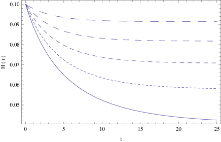
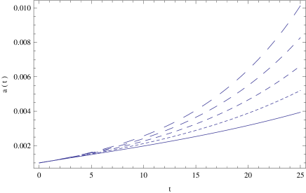
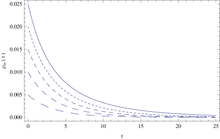
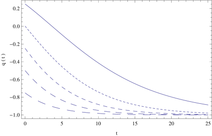
respectively. The time variation of the Hubble function $H$, of the scale factor $a$, of the matter energy density $\rho_{m}$, and of the deceleration parameter $q$, obtained by numerically integrating Eqs. (28) and (29) are represented, for different numerical values of the free parameters $\Lambda$, $\alpha$, $\beta$ and $\lambda$, in Figs. 1-5.

Figure 1: Time variation of the Hubble function $H(t)$ for the nonminimally matter coupled $f(T)$ gravity model with $f_{1}(T)=-\Lambda+\alpha_{1}T^{2}$ and $f_{2}(T)=\beta_{1}T^{2}$, or equivalently $f_{1}(H)=-\Lambda+\alpha H^{4}$ and $f_{2}(H)=\beta H^{4}$ with $\alpha=36\alpha_{1}$, $\beta=36\beta_{1}$, for five different choices of the parameters $\Lambda$, $\alpha$, $\beta$, and $\lambda$: $\Lambda=0.01$, $\alpha=0.16$, $\beta=0.1$, and $\lambda=1$ (solid curve), $\Lambda=0.02$, $\alpha=0.18$, $\beta=0.3$, and $\lambda=1.2$ (dotted curve), $\Lambda=0.03$, $\alpha=0.20$, $\beta=0.35$, and $\lambda=1.4$ (short-dashed curve), $\Lambda=0.04$, $\alpha=0.30$, $\beta=0.45$, and $\lambda=1.6$ (dashed curve), and $\Lambda=0.05$, $\alpha=0.40$, $\beta=0.55$, and $\lambda=1.8$ (long-dashed curve), respectively. The initial value for $H$ used to numerically integrate Eq. (29) is $H(0)=0.1$.

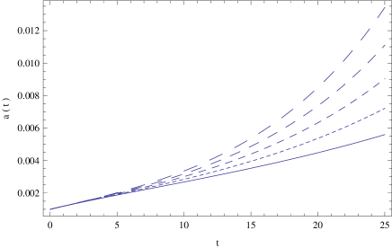
Figure 2: Time variation of of the scale factor $a(t)$ for the nonminimally matter coupled $f(T)$ gravity model with $f_{1}(T)=-\Lambda+\alpha_{1}T^{2}$ and $f_{2}(T)=\beta_{1}T^{2}$, or equivalently $f_{1}(H)=-\Lambda+\alpha H^{4}$ and $f_{2}(H)=\beta H^{4}$ with $\alpha=36\alpha_{1}$, $\beta=36\beta_{1}$, for five different choices of the parameters $\Lambda$, $\alpha$, $\beta$, and $\lambda$: $\Lambda=0.01$, $\alpha=0.16$, $\beta=0.1$, and $\lambda=1$ (solid curve), $\Lambda=0.02$, $\alpha=0.18$, $\beta=0.3$, and $\lambda=1.2$ (dotted curve), $\Lambda=0.03$, $\alpha=0.20$, $\beta=0.35$, and $\lambda=1.4$ (short-dashed curve), $\Lambda=0.04$, $\alpha=0.30$, $\beta=0.45$, and $\lambda=1.6$ (dashed curve), and $\Lambda=0.05$, $\alpha=0.40$, $\beta=0.55$, and $\lambda=1.8$ (long-dashed curve), respectively. The initial values for $a$ and $\dot{a}$ used to numerically integrate Eq. (29) are $a(0)=10^{-3}$ and $\dot{a}(0)=10^{-4}$, respectively.

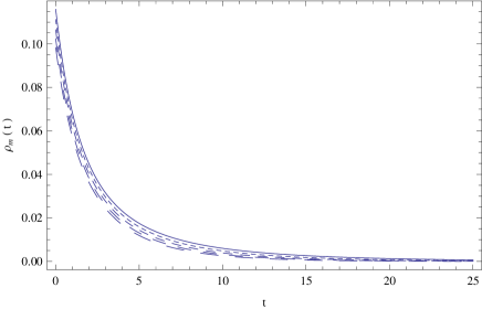
Figure 3: Time variation of the matter energy density $\rho_{m}(t)$ for the nonminimally matter coupled $f(T)$ gravity model with $f_{1}(T)=-\Lambda+\alpha_{1}T^{2}$ and $f_{2}(T)=\beta_{1}T^{2}$, or equivalently $f_{1}(H)=-\Lambda+\alpha H^{4}$ and $f_{2}(H)=\beta H^{4}$ with $\alpha=36\alpha_{1}$, $\beta=36\beta_{1}$, for five different choices of the parameters$\Lambda$, $\alpha$, $\beta$, and $\lambda$: $\Lambda=0.01$, $\alpha=0.16$, $\beta=0.1$, and $\lambda=1$ (solid curve), $\Lambda=0.02$, $\alpha=0.18$, $\beta=0.3$, and $\lambda=1.2$ (dotted curve), $\Lambda=0.03$, $\alpha=0.20$, $\beta=0.35$, and $\lambda=1.4$ (short-dashed curve), $\Lambda=0.04$, $\alpha=0.30$, $\beta=0.45$, and $\lambda=1.6$ (dashed curve), and $\Lambda=0.05$, $\alpha=0.40$, $\beta=0.55$, and $\lambda=1.8$ (long-dashed curve), respectively. The initial value for $H$ used to numerically integrate Eq. (29) is $H(0)=0.1$.

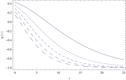
Figure 4: Time variation of the deceleration parameter $q(t)$ for the nonminimally matter coupled $f(T)$ gravity model with $f_{1}(T)=-\Lambda+\alpha_{1}T^{2}$ and $f_{2}(T)=\beta_{1}T^{2}$, or equivalently $f_{1}(H)=-\Lambda+\alpha H^{4}$ and $f_{2}(H)=\beta H^{4}$ with $\alpha=36\alpha_{1}$, $\beta=36\beta_{1}$, for five different choices of the parameters $\Lambda$, $\alpha$, $\beta$, and $\lambda$: $\Lambda=0.01$, $\alpha=0.16$, $\beta=0.1$, and $\lambda=1$ (solid curve), $\Lambda=0.02$, $\alpha=0.18$, $\beta=0.3$, and $\lambda=1.2$ (dotted curve), $\Lambda=0.03$, $\alpha=0.20$, $\beta=0.35$, and $\lambda=1.4$ (short-dashed curve), $\Lambda=0.04$, $\alpha=0.30$, $\beta=0.45$, and $\lambda=1.6$ (dashed curve), and $\Lambda=0.05$, $\alpha=0.40$, $\beta=0.55$, and $\lambda=1.8$ (long-dashed curve), respectively. The initial value for $H$ used to numerically integrate Eq. (29) is $H(0)=0.1$.

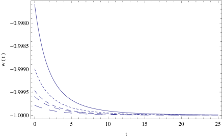
Figure 5: Time variation of the dark energy equation-of-state parameter $w_{DE}$ for the nonminimally matter coupled $f(T)$ gravity model with $f_{1}(T)=-\Lambda+\alpha_{1}T^{2}$ and $f_{2}(T)=\beta_{1}T^{2}$, or equivalently $f_{1}(H)=-\Lambda+\alpha H^{4}$ and $f_{2}(H)=\beta H^{4}$ with $\alpha=36\alpha_{1}$, $\beta=36\beta_{1}$, for five different choices of the parameters $\Lambda$, $\alpha$, $\beta$, and $\lambda$: $\Lambda=0.01$, $\alpha=0.16$, $\beta=0.1$, and $\lambda=1$ (solid curve), $\Lambda=0.02$, $\alpha=0.18$, $\beta=0.3$, and $\lambda=1.2$ (dotted curve), $\Lambda=0.03$, $\alpha=0.20$, $\beta=0.35$, and $\lambda=1.4$ (short dashed curve), $\Lambda=0.04$, $\alpha=0.30$, $\beta=0.45$, and $\lambda=1.6$ (dashed curve), and $\Lambda=0.05$, $\alpha=0.40$, $\beta=0.55$, and $\lambda=1.8$ (long dashed curve), respectively. The initial value for $H$ used to numerically integrate Eq. (29) is $H(0)=0.1$.

As depicted in Fig. 1, the Hubble function is a monotonically decreasing function of time for all $t>0$. In the limit of large times the Hubble function tends to a constant value, $\lim_{t\rightarrow\infty}H(t)=h_{0}={\rm constant}$. Hence, for the considered range of values of the free parameters, in the $f(T)$ model with torsion-matter coupling, the Universe ends its evolution in an accelerating, de Sitter-type phase. The scale factor $a$, shown in Fig. 2, indicates a monotonically time increase of the size of the Universe, and hence an expansionary behavior. The matter energy density, depicted in Fig. 3, tends progressively to zero. Furthermore, the deceleration parameter $q$, presented in Fig. 4, indicates a large variety of dynamical behaviors of the $f(T)$ model with matter-torsion coupling. In particular, for some values of the free parameters the Universe starts its evolution in the matter-dominated phase from a decelerating phase, and ends in a de Sitter-type accelerated behavior. Other values of the parameters produce Universe models starting from a marginally accelerating phase ($q=0$), and ending in a de Sitter state. Finally, for other parameter choices at the beginning of the matter dominated phase the Universe is already in an accelerating phase, that is with $q<0$. Lastly, as depicted in Fig. 5, for these specific choices of the parameters, the dark energy equation-of-state parameter $w_{DE}$ is very close to the value $-1$, to which it rigorously tends in the large time limits. This is an advantage, since in this model the effective torsion-matter coupling can successfully mimic the cosmological constant, in agreement with observations.

After the above numerical elaboration, we examine whether we can obtain analytical expressions in various limits. In particular, we analyze the properties of the equations in the limit of small and large $H(t)$, respectively.

IV.1.1 The limit of small $H$

In the limit of small $H(t)$, that is at the late phases of the cosmological evolution, Eq. (29) becomes

$$\dot{H}=\frac{1}{4}\left(\alpha\Lambda+\beta\lambda\Lambda^{2}-6\right)H^{2}+\frac{\Lambda}{4}$$ (30)

yielding the following solution

$$H(t)=\sqrt{H_{1}}\tan\left[\tan^{-1}\left(\frac{H_{0}}{\sqrt{H_{1}}}\right)+\frac{\Lambda}{4\sqrt{H_{1}}}\left(t-t_{0}\right)\right],$$ (31)

with $H_{1}=\Lambda/\left[\Lambda(\alpha+\beta\lambda\Lambda)-6\right]$, and where we have used the initial condition $H\left(t_{0}\right)=H_{0}$. Thus, the scale factor evolves according to

$$a(t)=a_{0}\cos^{-\frac{4H_{1}}{\Lambda}}\left[\tan^{-1}\left(\frac{H_{0}}{\sqrt{H_{1}}}\right)+\frac{\Lambda}{4\sqrt{H_{1}}}\left(t-t_{0}\right)\right],$$ (32)

where $a_{0}$ is an arbitrary constant of integration.

Similarly, the deceleration parameter (26) becomes

$$q(t)=-\frac{\Lambda\csc^{2}\left[\tan^{-1}\left(\frac{H_{0}}{\sqrt{H_{1}}}\right)+\frac{\Lambda\left(t-t_{0}\right)}{4\sqrt{H_{1}}}\right]}{4H_{1}}-1.$$ (33)

Additionally, the matter energy-density (28) can be approximated as

$$\rho_{m}(t)=3H(t)^{2}-\frac{\Lambda}{2},$$ (34)

and using Eq. (31) its explicit time dependence acquires the form

$$\rho_{m}(t)=3H_{1}\tan^{2}\left[\tan^{-1}\left(\frac{H_{0}}{\sqrt{H_{1}}}\right)+\frac{\Lambda\left(t-t_{0}\right)}{4\sqrt{H_{1}}}\right]-\frac{\Lambda}{2}.$$ (35)

Finally, the dark-energy equation-of-state parameter from (27), becomes

$$w_{DE}(t)=-1-(\alpha+\beta\lambda\Lambda)H(t)^{2},$$ (36)

that is

$$w_{DE}(t) = -1-(\alpha+\beta\lambda\Lambda)H_{1}\times$$ (37)

$$\!\!\times\tan^{2}\left[\tan^{-1}\left(\frac{H_{0}}{\sqrt{H_{1}}}\right)+\frac{\Lambda\left(t-t_{0}\right)}{4\sqrt{H_{1}}}\right].$$

Interestingly enough, we observe that according to the parameter values, $w_{DE}$ can be either above or below $-1$, that is the effective dark-energy sector can be quintessence-like or phantom-like. This feature, which is expected to happen in modified gravity Nojiri:2013ru , is an additional advantage of the scenario at hand.

Lastly, we mention that in the large-time limit the Hubble function (31) becomes almost constant, implying that a de Sitter-type evolution is possible in the framework of the present model.

IV.1.2 The limit of large $H$

In the limit of large $H$, corresponding to the early phases of the cosmological evolution, in the first order approximation the differential equation (29) describing the cosmological dynamics of the Hubble function becomes

$$\dot{H}=-\frac{3}{4}\alpha H^{4},$$ (38)

with the general solution given by

$$H(t)=\frac{2^{2/3}H_{0}}{\left[4+9H_{0}^{3}\alpha\left(t-t_{0}\right)\right]^{1/3}}.$$ (39)

The behavior of the scale factor can then be described by the equation

$$a(t)=\exp\left\{\frac{1}{{3\sqrt[3]{2}\alpha}}\left[\frac{4}{H_{0}^{3}}+9\alpha\left(t-t_{0}\right)\right]^{2/3}\right\},$$ (40)

that is, it is determined solely by the parameter $\alpha$. Similarly, the deceleration parameter (26) is given by

$$q(t)=\frac{3\alpha H_{0}^{2}}{\left[8+18\alpha H_{0}^{3}\left(t-t_{0}\right)\right]^{2/3}}-1.$$ (41)

Moreover, for the matter energy density (28) we obtain

$$\rho_{m}(t)=\frac{\alpha}{2\beta\lambda},$$ (42)

showing that during the time interval for which this approximation is valid the energy density of the matter is approximately constant. Finally, the dark-energy equation-of-state parameter from (27), becomes

$$w_{DE}(t)=-\frac{\alpha}{2}H(t)^{2}=-\frac{\alpha}{2}\frac{2^{4/3}H_{0}^{2}}{\left[4+9H_{0}^{3}\alpha\left(t-t_{0}\right)\right]^{2/3}}.$$ (43)

Again, we mention that according to the parameter choice, $w_{DE}$ can be either above or below $-1$, that is the effective dark-energy sector can be quintessence-like or phantom-like.

IV.2 $f_{1}(T)=-\Lambda$ and $f_{2}(T)=\alpha_{1}T+\beta_{1}T^{2}$

As a second example, we examine the case where $f_{1}(T)=-\Lambda$ and $f_{2}(T)=\alpha_{1}T+\beta_{1}T^{2}$, where $\Lambda>0$, $\alpha_{1}$ and $\beta_{1}$ are constants, since this scenario is also the first non-trivial correction to TEGR, that is to General Relativity. Equivalently, we impose $f_{1}(H)=-\Lambda$ and $f_{2}(H)=\alpha H^{2}+\beta H^{4}$, with $\alpha=-6\alpha_{1}$ and $\beta=36\beta_{1}$. For the derivatives of the functions $f_{1}(T)$ and $f_{2}(T)$ we obtain $f_{1}^{\prime}(T)=f_{1}^{\prime\prime}(T)=0$, $f_{2}^{\prime}(H)=-\alpha/6-\beta H^{2}/3$, and $f_{2}^{\prime\prime}(H)=\beta/18$. The basic evolution equations (24) and (25) in this case become

$$\rho_{m}(t)=\frac{\Lambda-6H^{2}}{2\alpha\lambda H^{2}+6\beta\lambda H^{4}-2},$$ (44)

and

$$\dot{H}(t)=\frac{3\left(\Lambda-6H^{2}\right)\left(\alpha\lambda H^{2}+3\beta\lambda H^{4}-1\right)}{2\left(\alpha\lambda\Lambda+6\beta\lambda H^{2}\left(\Lambda-3H^{2}\right)-6\right)},$$ (45)

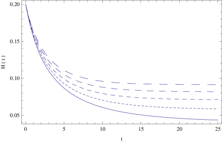
respectively. The time variation of the Hubble function $H$, of the scale factor $a$, of the matter density $\rho_{m}$, and of the deceleration parameter, obtained by numerically elaborating the system of Eqs. (44) and (45) for different values of the free parameters and assuming the matter to be dust ($w_{m}=0$), are presented in Figs. 6-10, respectively.

Figure 6: Time variation of the Hubble function $H(t)$ for the nonminimally matter coupled $f(T)$ gravity model with $f_{1}(T)=-\Lambda$ and $f_{2}(T)=\alpha_{1}T+\beta_{1}T^{2}$, or equivalently $f_{1}(H)=-\Lambda$ and $f_{2}(H)=\alpha H^{2}+\beta H^{4}$ with $\alpha=-6\alpha_{1}$, $\beta=36\beta_{1}$, for five different choices of the parameters $\Lambda$, $\alpha$, $\beta$, and $\lambda$: $\Lambda=0.01$, $\alpha=0.16$, $\beta=0.1$, and $\lambda=1$ (solid curve), $\Lambda=0.02$, $\alpha=0.18$, $\beta=0.3$, and $\lambda=1.2$ (dotted curve), $\Lambda=0.03$, $\alpha=0.20$, $\beta=0.35$, and $\lambda=1.4$ (short-dashed curve), $\Lambda=0.04$, $\alpha=0.30$, $\beta=0.45$, and $\lambda=1.6$ (dashed curve), and $\Lambda=0.05$, $\alpha=0.40$, $\beta=0.55$, and $\lambda=1.8$ (long-dashed curve), respectively. The initial value for $H$ used to numerically integrate Eq. (45) is $H(0)=0.2$.

Figure 7: Time variation of the scale factor $a(t)$ of the Universe for the nonminimally matter coupled $f(T)$ gravity model with $f_{1}(T)=-\Lambda$ and $f_{2}(T)=\alpha_{1}T+\beta_{1}T^{2}$, or equivalently $f_{1}(H)=-\Lambda$ and $f_{2}(H)=\alpha H^{2}+\beta H^{4}$ with $\alpha=-6\alpha_{1}$, $\beta=36\beta_{1}$, for five different choices of the parameters $\Lambda$, $\alpha$, $\beta$, and $\lambda$: $\Lambda=0.01$, $\alpha=0.16$, $\beta=0.1$, and $\lambda=1$ (solid curve), $\Lambda=0.02$, $\alpha=0.18$, $\beta=0.3$, and $\lambda=1.2$ (dotted curve), $\Lambda=0.03$, $\alpha=0.20$, $\beta=0.35$, and $\lambda=1.4$ (short-dashed curve), $\Lambda=0.04$, $\alpha=0.30$, $\beta=0.45$, and $\lambda=1.6$ (dashed curve), and $\Lambda=0.05$, $\alpha=0.40$, $\beta=0.55$, and $\lambda=1.8$ (long-dashed curve), respectively. The initial values for $a$ and $\dot{a}$ used to numerically integrate Eq. (45) are $a(0)=10^{-3}$ and $\dot{a}(0)=2\times 10^{-4}$, respectively.

Figure 8: Time variation of the matter energy density $\rho_{m}(t)$ of the Universe for the nonminimally matter coupled $f(T)$ gravity model with $f_{1}(T)=-\Lambda$ and $f_{2}(T)=\alpha_{1}T+\beta_{1}T^{2}$, or equivalently $f_{1}(H)=-\Lambda$ and $f_{2}(H)=\alpha H^{2}+\beta H^{4}$ with $\alpha=-6\alpha_{1}$, $\beta=36\beta_{1}$, for five different choices of the parameters $\Lambda$, $\alpha$, $\beta$, and $\lambda$: $\Lambda=0.01$, $\alpha=0.16$, $\beta=0.1$, and $\lambda=1$ (solid curve), $\Lambda=0.02$, $\alpha=0.18$, $\beta=0.3$, and $\lambda=1.2$ (dotted curve), $\Lambda=0.03$, $\alpha=0.20$, $\beta=0.35$, and $\lambda=1.4$ (short dashed curve), $\Lambda=0.04$, $\alpha=0.30$, $\beta=0.45$, and $\lambda=1.6$ (dashed curve), and $\Lambda=0.05$, $\alpha=0.40$, $\beta=0.55$, and $\lambda=1.8$ (long dashed curve), respectively. The initial value for $H$ used to numerically integrate Eq. (45) is $H(0)=0.2$.

Figure 9: Time variation of the deceleration parameter $q(t)$ of the Universe for the nonminimally matter coupled $f(T)$ gravity model with $f_{1}(T)=-\Lambda$ and $f_{2}(T)=\alpha_{1}T+\beta_{1}T^{2}$, or equivalently $f_{1}(H)=-\Lambda$ and $f_{2}(H)=\alpha H^{2}+\beta H^{4}$ with $\alpha=-6\alpha_{1}$, $\beta=36\beta_{1}$, for five different choices of the parameters $\Lambda$, $\alpha$, $\beta$, and $\lambda$: $\Lambda=0.01$, $\alpha=0.16$, $\beta=0.1$, and $\lambda=1$ (solid curve), $\Lambda=0.02$, $\alpha=0.18$, $\beta=0.3$, and $\lambda=1.2$ (dotted curve), $\Lambda=0.03$, $\alpha=0.20$, $\beta=0.35$, and $\lambda=1.4$ (short dashed curve), $\Lambda=0.04$, $\alpha=0.30$, $\beta=0.45$, and $\lambda=1.6$ (dashed curve), and $\Lambda=0.05$, $\alpha=0.40$, $\beta=0.55$, and $\lambda=1.8$ (long dashed curve), respectively. The initial value for $H$ used to numerically integrate Eq. (45) is $H(0)=0.2$.

Figure 10: Time variation of the dark energy equation of state parameter $w_{DE}$ of the Universe for the nonminimally matter coupled $f(T)$ gravity model with $f_{1}(T)=-\Lambda$ and $f_{2}(T)=\alpha_{1}T+\beta_{1}T^{2}$, or equivalently $f_{1}(H)=-\Lambda$ and $f_{2}(H)=\alpha H^{2}+\beta H^{4}$ with $\alpha=-6\alpha_{1}$, $\beta=36\beta_{1}$, for five different choices of the parameters $\Lambda$, $\alpha$, $\beta$, and $\lambda$: $\Lambda=0.01$, $\alpha=0.16$, $\beta=0.1$, and $\lambda=1$ (solid curve), $\Lambda=0.02$, $\alpha=0.18$, $\beta=0.3$, and $\lambda=1.2$ (dotted curve), $\Lambda=0.03$, $\alpha=0.20$, $\beta=0.35$, and $\lambda=1.4$ (short dashed curve), $\Lambda=0.04$, $\alpha=0.30$, $\beta=0.45$, and $\lambda=1.6$ (dashed curve), and $\Lambda=0.05$, $\alpha=0.40$, $\beta=0.55$, and $\lambda=1.8$ (long dashed curve), respectively. The initial value for $H$ used to numerically integrate Eq. (45) is $H(0)=0.2$.

The Hubble function, presented in Fig. 6, decreases monotonically in time, and tends to a constant value in the large-time limit. Therefore, for all the parameter choices the Universe ends in a de Sitter phase. The time variation of the scale factor, depicted in Fig. (7), indicates that all considered models are expanding. The matter energy density, shown in Fig. 8, monotonically decreases in time as expected. In the large-time limit the Universe ends in a vacuum state, with negligible matter density, and thus being completely dominated by the effective dark energy sector. The deceleration parameter, presented in Fig. 9 indicates a very strong dependence of the dynamical behavior of the Universe on the model parameters. For the considered values, in all cases at the beginning of the matter-dominated phase, the Universe is in a decelerating phase, with $q>0$. After a finite time $t_{a}$, determined by the condition $q\left(t_{a}\right)=0$, the Universe enters in an accelerated phase, with $q(t)<0,\forall t>t_{a}$. Similarly to the model of the previous subsection, the Universe always ends in a de Sitter phase, with $q=-1$. Finally, as depicted in Fig. 10, in the large time limit the dark energy equation-of-state parameter $w_{DE}$ tends to the value $-1$, namely $\lim_{t\rightarrow\infty}w_{DE}(t)=-1$, thus showing that this choice of the functions $f_{1}(T)$ and $f_{2}(T)$ can also successfully mimic an effective cosmological constant. Note however, that for these specific parameter choices $w_{DE}$ lies in the phantom regime, which is an advantage of the scenario at hand, revealing its capabilities.

After this numerical elaboration, we examine whether we can obtain analytical expressions in various limits. In particular, we examine the properties of the equations in the limit of small and large $H(t)$, respectively.

IV.2.1 The limit of small $H$

In the limit of small values of the Hubble function $H$, that is at late times, Eq. (45) can be approximated as

$$\dot{H}=\frac{3\Lambda}{2\left(6-\alpha\lambda\Lambda\right)}+\frac{3\left(\alpha^{2}\lambda^{2}\Lambda^{2}+6\beta\lambda\Lambda^{2}-36\right)}{2\left(6-\alpha\lambda\Lambda\right)^{2}}H^{2},$$ (46)

with the general solution given by

$$H(t)=\sqrt{H_{2}}\tan\left[\tan^{-1}\left(\frac{H_{0}}{\sqrt{H_{2}}}\right)+\frac{3\Lambda\left(t-t_{0}\right)}{2\left(6-\alpha\lambda\Lambda\right)\sqrt{H_{2}}}\right]$$ (47)

with $H_{2}=\Lambda(6-\alpha\lambda\Lambda)/\left(\alpha^{2}\lambda^{2}\Lambda^{2}+6\beta\lambda\Lambda^{2}-36\right)$, and where we have used the initial condition $H\left(t_{0}\right)=H_{0}$. The scale factor then becomes

$$a(t) = a_{0}\cos^{-\frac{2H_{2}(6-\alpha\lambda\Lambda)}{3\Lambda}}\times$$ (48)

$$\!\!\times\left[\tan^{-1}\left(\frac{H_{0}}{\sqrt{H_{2}}}\right)+\frac{3\Lambda\left(t-t_{0}\right)}{2\left(6-\alpha\lambda\Lambda\right)\sqrt{H_{2}}}\right],$$

where $a_{0}$ is an arbitrary constant of integration, while the deceleration parameter (26) behaves as

$$q(t)=-\frac{3\Lambda\csc^{2}\left[\tan^{-1}\left(\frac{H_{0}}{\sqrt{H_{2}}}\right)+\frac{3\Lambda\left(t-t_{0}\right)}{2\left(6-\alpha\lambda\Lambda\right)\sqrt{H_{2}}}\right]}{2\left(6-\alpha\lambda\Lambda\right)H_{2}}-1.$$ (49)

Note that in the limit of large $t$ the deceleration parameter tends to $-1$, $\lim_{t\rightarrow\infty}q(t)=-1$. Additionally, the matter density (44) becomes

$$\rho_{m}(t)=\left(3-\frac{\alpha\lambda\Lambda}{2}\right)H(t)^{2}-\frac{\Lambda}{2},$$ (50)

and using (47) we acquire

$$\rho_{m}(t) = -\frac{\Lambda}{2}+\left(3-\frac{\alpha\lambda\Lambda}{2}\right)H_{2}\times$$ (51)

$$\times\tan^{2}\left[\tan^{-1}\left(\frac{H_{0}}{\sqrt{H_{2}}}\right)+\frac{3\Lambda\left(t-t_{0}\right)}{2\left(6-\alpha\lambda\Lambda\right)\sqrt{H_{2}}}\right].$$

Finally, the dark-energy equation-of-state parameter from (27), becomes

$$w_{DE}(t) = -1+\frac{\alpha\lambda\Lambda}{\alpha\lambda\Lambda-6}-\frac{18\left(\alpha^{2}\lambda^{2}\Lambda+2\beta\lambda\Lambda-6\alpha\lambda\right)}{\left(6-\alpha\lambda\Lambda\right)^{2}}H^{2}$$ (52)

$$= -1+\frac{\alpha\lambda\Lambda}{\alpha\lambda\Lambda-6}-\frac{18\left(\alpha^{2}\lambda^{2}\Lambda+2\beta\lambda\Lambda-6\alpha\lambda\right)}{\left(6-\alpha\lambda\Lambda\right)^{2}}H_{2}$$

$$\times\tan^{2}\left[\tan^{-1}\left(\frac{H_{0}}{\sqrt{H_{2}}}\right)+\frac{3\Lambda\left(t-t_{0}\right)}{2\left(6-\alpha\lambda\Lambda\right)\sqrt{H_{2}}}\right].$$

which can lie both in the quintessence as well as in the phantom regime, depending on the specific choices of the free parameters of the model, namely on $\alpha$, $\beta$, $\lambda$ and $\Lambda$, respectively.

IV.2.2 The limit of large $H$

In the opposite limit of large $H$, that is at early times, at first order approximation Eq. (45) becomes

$$\dot{H}-\frac{3}{2}H^{2}=0,$$ (53)

with $H\left(t_{0}\right)=H_{0}$, and thus the general solution is given by

$$H(t)=\frac{2H_{0}}{2-3H_{0}\left(t-t_{0}\right)}.$$ (54)

The scale factor then reads

$$a(t)=a_{0}\left[\frac{2}{2-3H_{0}\left(t-t_{0}\right)}\right]^{2/3},$$ (55)

while the deceleration parameter is obtained as $q=-5/2$, that is the universe at early times always starts with acceleration, which corresponds to an inflationary stage. Finally, for the time variation of the matter energy density in the large-$H$ regime we find $\rho_{m}(t)\approx 0$, which is consistent with the interpretation of this stage as inflationary.

We mention that the above expressions for $H$, $a$, $q$ and $\rho_{m}$ at first order approximation, are independent on the free parameters of the model $\alpha$, $\beta$, $\lambda$ and $\Lambda$, respectively, and are determined only by the initial value of $H$ at $t=t_{0}$.

V Discussions and final remarks

In the present paper, we have considered an extension of the $f(T)$ gravity model by introducing a nonminimal coupling between torsion and matter. The geometric part of the action was extended through the introduction of two independent functions of the torsion scalar $T$, namely $f_{1}(T)$ and $f_{2}(T)$, respectively, with the function $f_{2}(T)$ being nonminimally coupled to the matter Lagrangian $L_{m}$. The resulting gravitational model presents some formal analogies with the nonminimally geometry-matter coupling introduced in Bertolami:2007gv . However, the resulting equations, as well as its physical and geometrical interpretations, are very different. The theory of nonminimal torsion-matter coupling is therefore a novel class of gravitational modification.

From the physical point of view, in this theory, matter is not just a passive component in the space-time continuum, but it plays an active role in the overall gravitational dynamics, which is strongly modified due to the supplementary interaction between matter and geometry. Moreover, the major advantage of the $f(T)$-type models, namely that the field equations are second order, is not modified by the torsion-matter coupling.

As an application of the nonminimal torsion-matter coupling scenario we have considered the dynamical evolution of a flat FRW universe. We have investigated the time dependence of the cosmologically relevant physical parameters, for two different choices of the functions $f_{1}(T)$ and $f_{2}(T)$, corresponding to the simplest departures from General Relativity. In these specific models the dynamics of the Universe is determined by the free parameters which appear in the functions $f_{1}(T)$ and $f_{2}(T)$, as well as by the matter-torsion coupling constant. Depending on the numerical values of these parameters a large number of cosmological behaviors can be obtained. In our analysis we have considered the matter dominated phase of the Universe evolution, that is, we neglected the matter pressure. More general models with $p_{m}$ can be easily constructed and analyzed.

We restricted our analysis in expanding evolutions, although contracting or bouncing solutions can be easily obtained as well. We have found a universe evolution in agreement with observations, that is a matter-dominated era followed by an accelerating phase. Additionally, the effective dark-energy equation-of-state parameter can lie in the quintessence or phantom regime, which reveals the capabilities of the scenario. Furthermore, a general and common property of the considered models is that they all end in a de Sitter phase, with zero matter density, that is to complete dark-energy domination. Finally, these models also accept solutions with almost constant Hubble function, which can describe the inflationary regime. Thus, the scenario of nonminimal torsion-matter coupling can offer a unified description of the universe evolution, from its inflationary to the late-time accelerated phases.

Apart from the exact numerical elaboration, we have extracted approximate analytical expressions in the limit of a small Hubble parameter, that is corresponding to the large-time limit, as well as for large Hubble parameters, that is corresponding to the beginning of the cosmological expansion. These expressions verify the above physical features that were extracted through the numerical analysis.

In conclusion, based on the torsional formulation of gravity, we have proposed a novel modified gravitational scenario which contains an arbitrary coupling between the torsion scalar and the matter Lagrangian. The cosmological implications of this theory proves to be very interesting. However, in order for the present scenario to be considered as a good candidate for the description of Nature, additional investigations should be performed, such as the detailed comparison with cosmological observations, the complete perturbation analysis, etc. These necessary studies lie beyond the scope of the present work and are left for future projects.

References

• (1) A. G. Riess et al., Astron. J.  116, 1009 (1998); S. Perlmutter et al., Astrophys. J.  517, 565 (1999).
• (2) E. J. Copeland, M. Sami and S. Tsujikawa, Int. J. Mod. Phys. D 15, 1753 (2006).
• (3) P. A. R. Ade et al. [Planck Collaboration], arXiv:1303.5062 [astro-ph.CO]; P. A. R. Ade et al. [Planck Collaboration], arXiv:1303.5076 [astro-ph.CO].
• (4) P. A. R Ade et al. [BICEP2 Collaboration], arXiv:1403.3985 [astro-ph.CO] (2014).
• (5) C. Bonvin, R. Durrer and R. Maartens, arXiv:1403.6768 [astro-ph.CO].
• (6) S. Lee, G. -C. Liu and K. -W. Ng, arXiv:1403.5585 [astro-ph.CO].
• (7) L. E. Strigari, Physics Reports 531, 1 (2013).
• (8) T. P. Sotiriou and V. Faraoni, Rev. Mod. Phys.  82, 451 (2010); A. De Felice and S. Tsujikawa, Living Rev. Rel. 13, 3 (2010); S. Nojiri and S. D. Odintsov, Phys. Rept. 505, 59 (2011).
• (9) C. G. Boehmer, T. Harko and F. S. N. Lobo, Astropart. Phys.  29, 386 (2008); C. G. Boehmer, T. Harko and F. S. N. Lobo, JCAP 0803, 024 (2008).
• (10) F. S. N. Lobo, Dark Energy-Current Advances and Ideas, 173-204, Research Signpost, ISBN 978 (2009) [arXiv:0807.1640 [gr-qc]].
• (11) R. Maartens, Living Rev. Rel.  7, 7 (2004).
• (12) O. Bertolami, C. G. Boehmer, T. Harko and F. S. N. Lobo, Phys. Rev. D 75, 104016 (2007).
• (13) O. Bertolami and J. Paramos, JCAP 1003, 009 (2010).
• (14) T. Harko, Phys. Lett. B 669, 376 (2008).
• (15) T. Harko and F. S. N. Lobo, Eur. Phys. J. C 70, 373 (2010).
• (16) T. Harko, F. S. N. Lobo, S. ’i. Nojiri and S. D. Odintsov, Phys. Rev. D 84, 024020 (2011).
• (17) Z. Haghani, T. Harko, F. S. N. Lobo, H. R. Sepangi, and S. Shahidi, Phys. Rev. D 88, 044023 (2013).
• (18) S. D. Odintsov and D. Sa´´a{\rm\acute{a}}ez-Gómez, Phys. Lett. B 725, 437 (2013).
• (19) S. Deser and G. W. Gibbons, Class. Quantum Grav. 15, L35 (1998).
• (20) A. Einstein 1928, Sitz. Preuss. Akad. Wiss. p. 217; ibid p. 224; A. Unzicker and T. Case, [physics/0503046].
• (21) C. Möller, Mat. Fys. Skr. Dan. Vid. Selsk. 1, 10 (1961); C. Pellegrini and J. Plebanski, Mat. Fys. Skr. Dan. Vid. Selsk. 2, 4 (1963).
• (22) K. Hayashi and T. Shirafuji, Phys. Rev.  D 19, 3524 (1979).
• (23) J. W. Maluf, Annalen Phys.  525, 339 (2013).
• (24) R. Aldrovandi and J. G. Pereira, Teleparallel Gravity: An Introduction (Springer, Dordrecht, 2013). J. G. Pereira, Teleparallelism: a new insight into gravitation, in Springer Handbook of Spacetime, ed. by A. Ashtekar and V. Petkov (Springer, Dordrecht, 2013).
• (25) R. Ferraro and F. Fiorini, Phys. Rev. D 75, 084031 (2007); G. R. Bengochea, & R. Ferraro, Phys. Rev. D, 79, 124019, (2009).
• (26) E. V. Linder, Phys. Rev. D 81, 127301 (2010).
• (27) S. H. Chen, J. B. Dent, S. Dutta and E. N. Saridakis, Phys. Rev. D 83, 023508 (2011); P. Wu, H. W. Yu, Phys. Lett. B693, 415 (2010); J. B. Dent, S. Dutta, E. N. Saridakis, JCAP 1101, 009 (2011); R. Zheng and Q. G. Huang, JCAP 1103, 002 (2011); K. Bamba, C. Q. Geng, C. C. Lee and L. W. Luo, JCAP 1101, 021 (2011); Y. -F. Cai, S. -H. Chen, J. B. Dent, S. Dutta, E. N. Saridakis, Class. Quant. Grav.  28, 2150011 (2011); M. Sharif, S. Rani, Mod. Phys. Lett.  A26, 1657 (2011); M. Li, R. X. Miao and Y. G. Miao, JHEP 1107, 108 (2011); S. Capozziello, V. F. Cardone, H. Farajollahi and A. Ravanpak, Phys. Rev.  D 84, 043527 (2011); M. H. Daouda, M. E. Rodrigues and M. J. S. Houndjo, Eur. Phys. J. C 72, 1890 (2012); Y. P. Wu and C. Q. Geng, Phys. Rev. D 86, 104058 (2012); H. Wei, X. J. Guo and L. F. Wang, Phys. Lett.  B 707, 298 (2012); K. Atazadeh and F. Darabi, Eur.Phys.J. C72 (2012) 2016; H. Farajollahi, A. Ravanpak and P. Wu, Astrophys. Space Sci.  338, 23 (2012); K. Karami and A. Abdolmaleki, JCAP 1204 (2012) 007; L. Iorio and E. N. Saridakis, Mon.Not.Roy.Astron.Soc. 427 (2012) 1555; V. F. Cardone, N. Radicella and S. Camera, Phys. Rev. D 85, 124007 (2012); M. Jamil, D. Momeni and R. Myrzakulov, Eur. Phys. J. C 72, 2267 (2012); Y. C. Ong, K. Izumi, J. M. Nester and P. Chen, Phys. Rev. D 88 (2013) 2, 024019; J. Amoros, J. de Haro and S. D. Odintsov, Phys. Rev. D 87, 104037 (2013); S. Nesseris, S. Basilakos, E. N. Saridakis and L. Perivolaropoulos, Phys. Rev. D 88, 103010 (2013); K. Bamba, S. Capozziello, M. De Laurentis, S. ’i. Nojiri and D. Sáez-Gómez, Phys. Lett. B 727, 194 (2013); S. Basilakos, S. Capozziello, M. De Laurentis, A. Paliathanasis and M. Tsamparlis, Phys. Rev. D 88, 103526 (2013); G. Otalora, arXiv:1402.2256 [gr-qc]; A. Paliathanasis, S. Basilakos, E. N. Saridakis, S. Capozziello, K. Atazadeh, F. Darabi and M. Tsamparlis, arXiv:1402.5935 [gr-qc]; G. G. L. Nashed, arXiv:1403.6937 [gr-qc]. Y. Kucukakca, Eur. Phys. J. C 73, 2327 (2013) H. M. Sadjadi, Phys. Rev. D 87, no. 6, 064028 (2013)
• (28) G. R. Bengochea, Phys. Lett.  B695, 405 (2011); T. Wang, Phys. Rev.  D84, 024042 (2011); R. -X. Miao, M. Li and Y. -G. Miao, JCAP 1111, 033 (2011); C. G. Boehmer, A. Mussa and N. Tamanini, Class. Quant. Grav.  28, 245020 (2011); M. H. Daouda, M. E. Rodrigues and M. J. S. Houndjo, Eur. Phys. J. C 71, 1817 (2011); R. Ferraro, F. Fiorini, Phys. Rev. D 84, 083518 (2011); P. A. Gonzalez, E. N. Saridakis and Y. Vasquez, JHEP 1207, 053 (2012); S. Capozziello, P. A. Gonzalez, E. N. Saridakis and Y. Vasquez, JHEP 1302 (2013) 039; K. Atazadeh and M. Mousavi, Eur. Phys. J. C 72, 2272 (2012).
• (29) G. Kofinas and E. N. Saridakis, arXiv:1404.2249 [gr-qc].
• (30) Z. Haghani, T. Harko, H. R. Sepangi, and S. Shahidi, JCAP 10, 061 (2012).
• (31) Z. Haghani, T. Harko, H. R. Sepangi, and S. Shahidi, Phys. Rev. D 88, 044024 (2013).
• (32) Weitzenböck R., Invarianten Theorie, Nordhoff, Groningen (1923).
• (33) J. W. Maluf, J. Math. Phys. 35 (1994) 335; H. I. Arcos and J. G. Pereira, Int. J. Mod. Phys. D 13, 2193 (2004).
• (34) C. -Q. Geng, C. -C. Lee, E. N. Saridakis, Y. -P. Wu, Phys. Lett.  B704, 384 (2011); H. Wei, Phys. Lett. B 712, 430 (2012); C. -Q. Geng, C. -C. Lee, E. N. Saridakis, JCAP 1201, 002 (2012); C. Xu, E. N. Saridakis and G. Leon, JCAP 1207, 005 (2012); G. Otalora, Phys. Rev. D 88, 063505 (2013); C. -Q. Geng, J. -A. Gu and C. -C. Lee, Phys. Rev. D 88, 024030 (2013); G. Otalora, JCAP 1307, 044 (2013).
• (35) Oeyvind Groen and Sigbjorn Hervik, Einstein’s general theory of relativity, New York, USA: Springer (2007).
• (36) O. Bertolami, F. S. N. Lobo and J. Paramos, Phys. Rev. D 78, 064036 (2008); O. Bertolami, J. Paramos, T. Harko and F. S. N. Lobo, arXiv:0811.2876 [gr-qc].
• (37) S. ’i. Nojiri and E. N. Saridakis, Astrophys. Space Sci.  1, 2013 (347).