Planck 2013 results. XVI. Cosmological parameters

Abstract: This paper presents the first cosmological results based on Planck measurements of the cosmic microwave background (CMB) temperature and lensing-potential power spectra. We find that the Planck spectra at high multipoles ($\ell\mathrel{\raise 1.72218pt\hbox{\hbox to0.0pt{$>$\hss}\lower 5.16663pt\hbox{$\sim$}}}40$) are extremely well described by the standard spatially-flat six-parameter $\Lambda$CDM cosmology with a power-law spectrum of adiabatic scalar perturbations. Within the context of this cosmology, the Planck data determine the cosmological parameters to high precision: the angular size of the sound horizon at recombination, the physical densities of baryons and cold dark matter, and the scalar spectral index are estimated to be $\theta_{\ast}=(1.04147\pm 0.00062)\times 10^{-2}$, $\Omega_{\rm b}h^{2}=0.02205\pm 0.00028$, $\Omega_{\rm c}h^{2}=0.1199\pm 0.0027$, and $n_{\rm s}=0.9603\pm 0.0073$, respectively (Note that in this abstract we quote 68% errors on measured parameters and 95% upper limits on other parameters.) For this cosmology, we find a low value of the Hubble constant, $H_{0}=(67.3\pm 1.2)\thinspace{\rm km}\thinspace{\rm s}^{-1}\thinspace{\rm Mpc}^{-1}$, and a high value of the matter density parameter, $\Omega_{\rm m}=0.315\pm 0.017$. These values are in tension with recent direct measurements of $H_{0}$ and the magnitude-redshift relation for Type Ia supernovae, but are in excellent agreement with geometrical constraints from baryon acoustic oscillation (BAO) surveys. Including curvature, we find that the Universe is consistent with spatial flatness to percent level precision using Planck CMB data alone. We use high-resolution CMB data together with Planck to provide greater control on extragalactic foreground components in an investigation of extensions to the six-parameter $\Lambda$CDM model. We present selected results from a large grid of cosmological models, using a range of additional astrophysical data sets in addition to Planck and high-resolution CMB data. None of these models are favoured over the standard six-parameter $\Lambda$CDM cosmology. The deviation of the scalar spectral index from unity is insensitive to the addition of tensor modes and to changes in the matter content of the Universe. We find an upper limit of $r_{0.002}<0.11$ on the tensor-to-scalar ratio. There is no evidence for additional neutrino-like relativistic particles beyond the three families of neutrinos in the standard model. Using BAO and CMB data, we find $N_{\rm eff}=3.30\pm 0.27$ for the effective number of relativistic degrees of freedom, and an upper limit of $0.23\thinspace{\rm eV}$ for the sum of neutrino masses. Our results are in excellent agreement with big bang nucleosynthesis and the standard value of $N_{\rm eff}=3.046$. We find no evidence for dynamical dark energy; using BAO and CMB data, the dark energy equation of state parameter is constrained to be $w=-1.13^{+0.13}_{-0.10}$. We also use the Planck data to set limits on a possible variation of the fine-structure constant, dark matter annihilation and primordial magnetic fields. Despite the success of the six-parameter $\Lambda$CDM model in describing the Planck data at high multipoles, we note that this cosmology does not provide a good fit to the temperature power spectrum at low multipoles. The unusual shape of the spectrum in the multipole range $20\la\ell\la 40$ was seen previously in the WMAP data and is a real feature of the primordial CMB anisotropies. The poor fit to the spectrum at low multipoles is not of decisive significance, but is an “anomaly” in an otherwise self-consistent analysis of the Planck temperature data.

1 Introduction

The discovery of the cosmic microwave background (CMB) by Penzias & Wilson (1965) established the modern paradigm of the hot big bang cosmology. Almost immediately after this seminal discovery, searches began for anisotropies in the CMB – the primordial signatures of the fluctuations that grew to form the structure that we see today. After a number of earlier detections, convincing evidence for a dipole anisotropy was reported by Smoot et al. (1977), but despite many attempts, the detection of higher-order anisotropies proved elusive until the first results from the Cosmic Background Explorer (COBE; Smoot et al. 1992). The COBE results established the existence of a nearly scale-invariant spectrum of primordial fluctuations on angular scales larger than $7^{\circ}$, consistent with the predictions of inflationary cosmology, and stimulated a new generation of precision measurements of the CMB of which this set of papers forms a part.

CMB anisotropies are widely recognized as one of the most powerful probes of cosmology and early-Universe physics. Given a set of initial conditions and assumptions concerning the background cosmology, the angular power spectrum of the CMB anisotropies can be computed numerically to high precision using linear perturbation theory (see Sect. 2). The combination of precise experimental measurements and accurate theoretical predictions can be used to set tight constraints on cosmological parameters. The influential results from the Wilkinson Microwave Anisotropy Probe (WMAP) satellite (Bennett et al. 2003; Spergel et al. 2003), following on from earlier ground-based and sub-orbital experiments, demonstrated the power of this approach, which has been followed by all subsequent CMB experiments.

Figure 1: Planck foreground-subtracted temperature power spectrum (with foreground and other “nuisance” parameters fixed to their best-fit values for the base $\Lambda$CDM model). The power spectrum at low multipoles ($\ell=2$–$49$, plotted on a logarithmic multipole scale) is determined by the Commander algorithm applied to the Planck maps in the frequency range $30$–$353$ GHz over 91% of the sky. This is used to construct a low-multipole temperature likelihood using a Blackwell-Rao estimator, as described in Planck Collaboration XV (2014). The asymmetric error bars show 68% confidence limits and include the contribution from uncertainties in foreground subtraction. At multipoles $50\leq\ell\leq 2500$ (plotted on a linear multipole scale) we show the best-fit The CMB spectrum computed from the CamSpec likelihood (see Planck Collaboration XV 2014) after removal of unresolved foreground components. This spectrum is averaged over the frequency range $100$–$217\thinspace{\rm GHz}$ using frequency-dependent diffuse sky cuts (retaining 58% of the sky at 100 GHz and 37% of the sky at $143$ and $217\thinspace{\rm GHz}$) and is sample-variance limited to $\ell\sim 1600$. The light grey points show the power spectrum multipole-by-multipole. The blue points show averages in bands of width $\Delta\ell\approx 31$ together with $1\thinspace\sigma$ errors computed from the diagonal components of the band-averaged covariance matrix (which includes contributions from beam and foreground uncertainties). The red line shows the temperature spectrum for the best-fit base $\Lambda$CDM cosmology. The lower panel shows the power spectrum residuals with respect to this theoretical model. The green lines show the $\pm 1\thinspace\sigma$ errors on the individual power spectrum estimates at high multipoles computed from the CamSpec covariance matrix. Note the change in vertical scale in the lower panel at $\ell=50$.

Planck is the third-generation space mission, following COBE and WMAP, dedicated to measurements of the CMB anistropies. The primary aim of Planck (Planck Collaboration 2005) is to measure the temperature and polarization anisotropies with micro-Kelvin sensitivity per resolution element over the entire sky. The wide frequency coverage of Planck (30–857 GHz) was chosen to provide accurate discrimination of Galactic emission from the primordial anisotropies and to enable a broad range of ancilliary science, such as detections of galaxy clusters, extragalactic point sources and the properties of Galactic dust emission. This paper, one of a set associated with the 2013 release of data from the Planck mission (Planck Collaboration I 2014), describes the first cosmological parameter results from the Planck temperature power spectrum.

The results from WMAP (see Bennett et al. 2012 and Hinshaw et al. 2012 for the final nine-year WMAP results) together with those from high-resolution ground-based CMB experiments (e.g., Reichardt et al. 2012; Story et al. 2012; Sievers et al. 2013) are remarkably consistent with the predictions of a “standard” cosmological model. This model is based upon a spatially-flat, expanding Universe whose dynamics are governed by General Relativity and whose constituents are dominated by cold dark matter (CDM) and a cosmological constant ($\Lambda$) at late times. The primordial seeds of structure formation are Gaussian-distributed adiabatic fluctuations with an almost scale-invariant spectrum. This model (which will be referred to as the base $\Lambda$CDM model in this paper) is described by only six key parameters. Despite its simplicity, the base $\Lambda$CDM model has proved to be successful in describing a wide range of cosmological data in addition to the CMB, including the Type Ia supernovae magnitude-distance relation, baryon acoustic oscillation measurements, the large-scale clustering of galaxies and cosmic shear (as reviewed in Sect. 5).

Nevertheless, there have been some suggestions of new physics beyond that assumed in the base $\Lambda$CDM model. Examples include various large-angle “anomalies” in the CMB (as reviewed by the WMAP team in Bennett et al. 2011) and hints of new physics, such as additional relativistic particles, that might steepen the high multipole “damping tail” of the CMB temperature power spectrum (Dunkley et al. 2011; Hou et al. 2012). Furthermore, developments in early-Universe cosmology over the last 20 years or so have led to a rich phenomenology (see e.g., Baumann 2009 for a review). It is easy to construct models that preserve the main features of simple single-field inflationary models, but lead to distinctive observational signatures such as non-Gaussianity, isocurvature modes or topological defects.

A major goal of the Planck experiment is to test the $\Lambda$CDM model to high precision and identify areas of tension. From previous CMB experiments and other cosmological probes, we know that any departures from the standard six-parameter $\Lambda$CDM cosmology are likely to be small and challenging to detect. Planck, with its combination of high sensitivity, wide frequency range and all-sky coverage, is uniquely well-suited to this challenge.

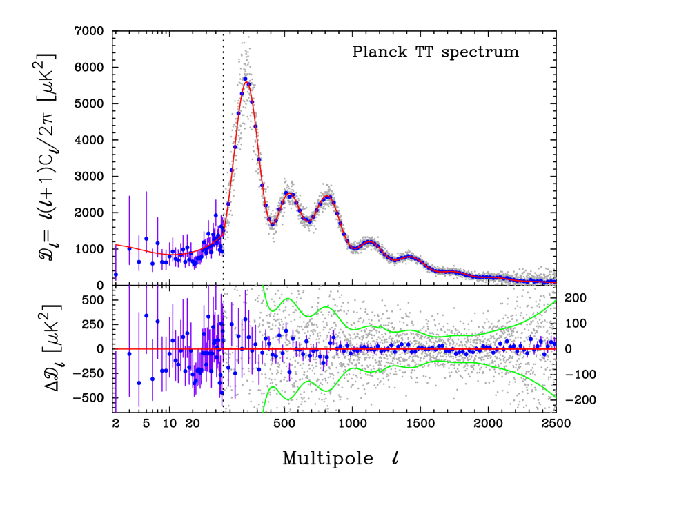
The focus of this paper is to investigate cosmological constraints from the temperature power spectrum measured by Planck. Figure 1 summarizes some important aspects of the Planck temperature power spectrum; we plot this as ${\cal D}_{\ell}\equiv\ell(\ell+1)C_{\ell}/2\pi$ (a notation we will use throughout this paper) versus multipole $\ell$. The temperature likelihood used in this paper is a hybrid: over the multipole range $\ell=2$–$49$, the likelihood is based on a component-separation algorithm applied to 91% of the sky (Planck Collaboration XII 2014; Planck Collaboration XV 2014). The likelihood at higher multipoles is constructed from cross-spectra over the frequency range 100–217 GHz, as discussed in Planck Collaboration XV (2014). It is important to recognize that unresolved foregrounds (and other factors such as beams and calibration uncertainties) need to be modelled to high precision to achieve the science goals of this paper. There is therefore no unique “Planck primordial temperature spectrum”. Figure 1 is based on a full likelihood solution for foreground and other “nuisance” parameters assuming a cosmological model. A change in the cosmology will lead to small changes in the Planck primordial CMB power spectrum because of differences in the foreground solution. Neverthess, Fig. 1 provides a good illustration of the precision achieved by Planck. The precision is so high that conventional power spectrum plots (shown in the upper panel of Fig. 1) are usually uninformative. We therefore place high weight in this paper on plots of residuals with respect to the best-fit model (shown in the lower panel). Figure 1 also serves to illustrate the highly interconnected nature of this series of papers. The temperature likelihood used in this paper utilizes data from both the Planck Low Frequency Instrument (LFI) and High Frequency Instrument (HFI). The data-processing chains for these two instruments and beam calibrations are described in Planck Collaboration II (2014), Planck Collaboration VI (2014), and associated papers (Planck Collaboration III 2014; Planck Collaboration IV 2014; Planck Collaboration V 2014; Planck Collaboration VII 2014; Planck Collaboration VIII 2014; Planck Collaboration IX 2014; Planck Collaboration X 2014). Component separation is described in Planck Collaboration XII (2014) and the temperature power spectrum and likelihood, as used in this paper, are described in Planck Collaboration XV (2014). Planck Collaboration XV (2014) also presents a detailed analysis of the robustness of the likelihood to various choices, such as frequency ranges and sky masks (and also compares the likelihood to results from an independent likelihood code based on different assumptions, see also Appendix C). Consistency of the Planck maps across frequencies is demonstrated in Planck Collaboration XXXI (2014), and the level of consistency with WMAP is assessed.

This paper is closely linked to other papers reporting cosmological results in this series. We make heavy use of the gravitational lensing power spectrum and likelihood estimated from an analysis of the 4-point function of the Planck maps (Planck Collaboration XVII 2014). The present paper concentrates on simple parameterizations of the spectrum of primordial fluctuations. Tests of specific models of inflation, isocurvature modes, broken scale-invariance etc. are discussed in Planck Collaboration XXII (2014). Here, we assume throughout that the initial fluctuations are Gaussian and statistically isotropic. Precision tests of non-Gaussianity, from Planck estimates of the 3- and 4-point functions of the temperature anisotropies, are presented in Planck Collaboration XXIV (2014). Tests of isotropy and additional tests of non-Gaussianity using Planck data are discussed in Planck Collaboration XXIII (2014) and Planck Collaboration XXVI (2014).

The outline of the paper is as follows. In Sect. 2 we define our notation and cosmological parameter choices. This section also summarizes aspects of the Markov chain Monte Carlo (MCMC) sampler used in this paper and of the CMB Boltzmann code used to predict theoretical temperature power spectra. Section 3 presents results on cosmological parameters using Planck data alone. For this data release we do not use Planck polarization data in the likelihood, and we therefore rely on WMAP polarization data at low multipoles to constrain the optical depth, $\tau$, from reionization. An interesting aspect of Sect. 3 is to assess whether CMB gravitational lensing measurements from Planck can be used to constrain the optical depth without the use of WMAP polarization measurements.

Section 4 introduces additional CMB temperature data from high-resolution experiments. This section presents a detailed description of how we have modified the Planck model for unresolved foreground and “nuisance” parameters introduced in Planck Collaboration XV (2014) to enable the Planck spectra to be used together with those from other CMB experiments. Combining high-resolution CMB experiments with Planck mitigates the effects of unresolved foregrounds which, as we will show, can affect cosmological parameters (particularly for extensions to the base $\Lambda$CDM model) if the foreground parameters are allowed too much freedom. Section 4 ends with a detailed analysis of whether the base $\Lambda$CDM model provides an acceptable fit to the CMB temperature power spectra from Planck and other experiments.

It is well known that certain cosmological parameter combinations are highly degenerate using CMB power spectrum measurements alone (Zaldarriaga et al. 1997; Efstathiou & Bond 1999; Howlett et al. 2012). These degeneracies can be broken by combining with other cosmological data (though the Planck lensing analysis does help to break the principal “geometrical” degeneracy, as discussed in Sect. 5.1). Section 5 discusses additional “astrophysical” data that are used in combination with Planck. Since the Planck temperature data are so precise, we have been selective in the additional data sets that we have chosen to use. Section 5 discusses our rationale for making these choices.

Having made a thorough investigation of the base $\Lambda$CDM model, Sect. 6 describes extended models, including models with non-power-law spectral indices, tensor modes, curvature, additional relativistic species, neutrino masses and dynamical dark energy. This section also discusses constraints on models with annihilating dark matter, primordial magnetic fields and a time-variable fine-structure constant.

Finally, we present our conclusions in Sect. 7. Appendix A compares the Planck and WMAP base $\Lambda$CDM cosmologies. Appendix B contrasts the Planck best-fit $\Lambda$CDM cosmology with that determined recently by combining data from the South Pole Telescope with WMAP (Story et al. 2012). Appendix C discusses the dependence of our results for extended models on foreground modelling and likelihood choices, building on the discussion in Planck Collaboration XV (2014) for the base $\Lambda$CDM model.

Since the appearance of the first draft of this paper, there have been a number of developments that affect both the Planck data and some of the constraints from supplementary astrophysical data used in this paper.

The primary developments are as follows. [1] After the submission of this paper, we discovered a minor error in the ordering of the beam transfer functions applied to each of the CamSpec $217\times 217\thinspace{\rm GHz}$ cross-spectra before their coaddition to form a single spectrum. Correcting for this error changes the mean $217\times 217\thinspace{\rm GHz}$ spectrum by a smooth function with an amplitude of a few $(\mu\rm{K})^{2}$. An extensive analysis of a revised likelihood showed that this error has negligible impact on cosmological parameters and that it is absorbed by small shifts in the foreground parameters. Since the effect is so minor, we have decided not to change any of the numbers in this paper and not to revise the public version of the CamSpec likelihood. [2] The foreground-corrected $217\times 217\thinspace{\rm GHz}$ spectrum shows a small negative residual (or “dip”) with respect to the best-fit base $\rm{\Lambda CDM}$ theoretical model at multipoles $\ell\approx 1800$. This can be seen most clearly in Fig. 7 in this paper. After submission of this paper we found evidence that this feature is a residual systematic in the data associated with incomplete 4 K line removal (see Planck Collaboration VI 2014 for a discussion of the 4 K line removal algorithm). The 4 K lines, at specific frequencies in the detector timelines, are caused by an electromagnetic-interference/electromagnetic-compatibility (EMI-EMC) problem between the ${}^{4}{\rm He}$ Joule-Thomson (4 K) cooler drive electronics and the read-out electronics. This interference is time-variable. Tests in which we have applied more stringent flagging of 4 K lines show that the $\ell=1800$ feature is reduced to negligible levels in all sky surveys, including Survey 1 in which the effect is strongest. The 2014 Planck data release will include improvements in the 4 K line removal. It is important to emphasise that this systematic is a small effect. Analysis of cosmological parameters, removing the multipole range around $\ell=1800$ (and also analysis of the full mission data, where the effect is diluted by the additional sky surveys) shows that the impact of this feature on cosmological parameters is small (i.e., less than half a standard deviation) even for extensions to the base $\rm{\Lambda CDM}$ cosmology. Some quantitiative tests of the impact of this systematic on cosmology are summarized in Appendix C. [3] An error was found in the dark energy model used for theoretical predictions with equation of state $w\neq-1$, leading to few-percent $C_{\ell}$ errors at very low multipoles in extreme models with $w\mathrel{\raise 1.72218pt\hbox{\hbox to0.0pt{$>$\hss}\lower 5.16663pt\hbox{$\sim$}}}-0.5$. We have checked, using the corrected October 2013 camb version, that this propagates to only a very small error on marginalized parameters and that the results presented in this paper are consistent to within the stated numerical accuracy. [4] After this paper was submitted, Humphreys et al. (2013) presented the final results of a long-term campaign to establish a new geometric maser distance to NGC4258. Their revised distance of $(7.60\pm 0.23)\thinspace{\rm Mpc}$ leads to a lowering of the Hubble constant, based on the Cepheid distance scale, to $H_{0}=(72.0\pm 3.0)\thinspace{\rm km}\thinspace{\rm s}^{-1}\thinspace{\rm Mpc}^{-1}$, partially alleviating the tension between the Riess et al. (2011) results and the Planck results on $H_{0}$ discussed in Sect. 5.3 and subsequent sections. [5] In a recent paper, Betoule et al. (2013) present results from an extensive programme that improves the photometric calibrations of the SDSS and SNLS supernovae surveys. An analysis of the SDSS-II and SNLS supernovae samples, including revisions to the photometric calibrations, favours a higher value of $\Omega_{\rm m}=0.295\pm 0.034$ for the base $\rm{\Lambda CDM}$ model, consistent with the Planck results discussed in Sect. 5.4 (Betoule et al. 2014).

A detailed discussion of the impact of the changes discussed here on cosmology will be deferred until the Planck 2014 data release, which will include improvements to the low-level data processing and, by which time, improved complementary astrophysical data sets (such as a revised SNLS compilation) should be available to us. In revising this paper, we have taken the view that this, and other Planck papers in this 2013 release, should be regarded as a snapshot of the Planck analysis as it was in early 2013. We have therefore kept revisions to a minimum. Nevertheless, readers of this paper, and users of products from the Planck Legacy Archive (such as parameter tables and MCMC chains), should be aware of developments since the first submission of this paper.

2 Model, parameters, and methodology

Table 1: Cosmological parameters used in our analysis. For each, we give the symbol, prior range, value taken in the base $\Lambda$CDM cosmology (where appropriate), and summary definition (see text for details). The top block contains parameters with uniform priors that are varied in the MCMC chains. The ranges of these priors are listed in square brackets. The lower blocks define various derived parameters.

Parameter Prior range       Baseline       Definition $$\omega_{\mathrm{b}}\equiv\Omega_{\mathrm{b}}h^{2} [0.005,0.1] \ldots \omega_{\mathrm{c}}\equiv\Omega_{\mathrm{c}}h^{2} [0.001,0.99] \ldots 100\theta_{\mathrm{MC}} [0.5,10.0] \ldots 100\thinspace{\times} r_{\ast}/D_{\rm A} \tau [0.01,0.8] \ldots \Omega_{K} [-0.3,0.3] \Omega_{\mathrm{tot}}=1-\Omega_{K} \sum m_{\nu} [0,5] 0.06 m_{\nu,\thinspace\mathrm{sterile}}^{\mathrm{eff}} [0,3] w_{0} [-3.0,-0.3] -1 w(a)=w_{0}+(1-a)w_{a} w_{a} [-2,2] N_{\rm eff} [0.05,10.0] Y_{\text{P}} [0.1,0.5] A_{\rm L} [0,10] n_{\rm s} [0.9,1.1] \ldots k_{0}=0.05\text{Mpc}^{-1} n_{\rm t} n_{\rm t}=-r_{0.05}/8 k_{0}=0.05\text{Mpc}^{-1} dn_{\rm s}/d\ln k [-1,1] \ln(10^{10}A_{\rm s}) [2.7,4.0] \ldots k_{0}=0.05\thinspace\text{Mpc}^{-1} r_{0.05} [0,2] k_{0}=0.05\thinspace\text{Mpc}^{-1} \Omega_{\Lambda} \ldots t_{0} \ldots \Omega_{\mathrm{m}} \ldots \sigma_{8} \ldots z_{\text{re}} \ldots H_{0} \ldots \rm{km}\thinspace\rm{s}^{-1}\text{Mpc}^{-1} r_{0.002} k_{0}=0.002\thinspace\text{Mpc}^{-1} 10^{9}A_{\rm s} \ldots 10^{9}\thinspace\times k_{0}=0.05\thinspace\text{Mpc}^{-1} \omega_{\mathrm{m}}\equiv\Omega_{\mathrm{m}}h^{2} \ldots z_{\ast} \ldots r_{\ast}=r_{\rm s}(z_{\ast}) \ldots z=z_{\ast} 100\theta_{\ast} \ldots 100\thinspace\times z=z_{\ast} r_{\ast}/D_{\rm A}) z_{\rm drag} \ldots r_{\rm drag}=r_{\rm s}(z_{\rm drag}) \ldots z=z_{\rm drag} k_{\rm D} \ldots \text{Mpc}^{-1} 100\theta_{\rm D} \ldots 100\thinspace\times z_{\text{eq}} \ldots 100\theta_{\rm eq} \ldots 100\thinspace\times r_{\rm drag}/D_{\mathrm{V}}(0.57) \ldots z=0.57$$.              Baryon density today .              Cold dark matter density today .               approximation to (CosmoMC) .              Thomson scattering optical depth due to reionization .       0       Curvature parameter today with .              The sum of neutrino masses in eV .       0       Effective mass of sterile neutrino in eV .              Dark energy equation of state^a, .       0       As above (perturbations modelled using PPF) .       3.046       Effective number of neutrino-like relativistic degrees of freedom (see text) .       BBN       Fraction of baryonic mass in helium .       1       Amplitude of the lensing power relative to the physical value .              Scalar spectrum power-law index () .       Inflation       Tensor spectrum power-law index () .       0       Running of the spectral index .              Log power of the primordial curvature perturbations () .       0       Ratio of tensor primordial power to curvature power at .              Dark energy density divided by the critical density today .              Age of the Universe today (in Gyr) .              Matter density (inc. massive neutrinos) today divided by the critical density .              RMS matter fluctuations today in linear theory .              Redshift at which Universe is half reionized . [20,100]              Current expansion rate in .       0       Ratio of tensor primordial power to curvature power at .               dimensionless curvature power spectrum at .              Total matter density today (inc. massive neutrinos) .              Redshift for which the optical depth equals unity (see text) .              Comoving size of the sound horizon at .               angular size of sound horizon at ( .              Redshift at which baryon-drag optical depth equals unity (see text) .              Comoving size of the sound horizon at .              Characteristic damping comoving wavenumber () .               angular extent of photon diffusion at last scattering (see text) .              Redshift of matter-radiation equality (massless neutrinos) .               angular size of the comoving horizon at matter-radiation equality .              BAO distance ratio at (see Sect. 5.2)

$${}^{\textit{a}} w w_{0}$$For dynamical dark energy models with constant equation of state, we denote the equation of state by and adopt the same prior as for .

2.1 Theoretical model

We shall treat anisotropies in the CMB as small fluctuations about a Friedmann-Robertson-Walker metric whose evolution is described by General Relativity. We shall not consider modified gravity scenarios or “active” sources of fluctuations such as cosmic defects. The latter are discussed in  Planck Collaboration XXV (2014). Under our assumptions, the evolution of the perturbations can be computed accurately using a CMB Boltzmann code once the initial conditions, ionization history and constituents of the Universe are specified. We discuss each of these in this section, establishing our notation. Our conventions are consistent with those most commonly adopted in the field and in particular with those used in the camb Boltzmann code (Lewis et al. 2000), which is the default code used in this paper.

2.1.1 Matter and radiation content

We adopt the usual convention of writing the Hubble constant at the present day as $H_{0}=100\thinspace h\thinspace{\rm km}\thinspace{\rm s}^{-1}\thinspace{\rm Mpc}^{-1}$. For our baseline model, we assume that the cold dark matter is pressureless, stable and non-interacting, with a physical density $\omega_{\rm c}\equiv\Omega_{\mathrm{c}}h^{2}$. The baryons, with density $\omega_{\rm b}\equiv\Omega_{\mathrm{b}}h^{2}$, are assumed to consist almost entirely of hydrogen and helium; we parameterize the mass fraction in helium by $Y_{\text{P}}$. The process of standard big bang nucleosynthesis (BBN) can be accurately modelled, and gives a predicted relation between $Y_{\text{P}}$, the photon-baryon ratio, and the expansion rate (which depends on the number of relativistic degrees of freedom). By default we use interpolated results from the PArthENoPE BBN code (Pisanti et al. 2008) to set $Y_{\text{P}}$, following Hamann et al. (2011), which for the Planck best-fitting base model (assuming no additional relativistic components and negligible neutrino degeneracy) gives $Y_{\text{P}}=0.2477$. We shall compare our results with the predictions of BBN in Sect. 6.4.

The photon temperature today is well measured to be $T_{0}=2.7255\pm 0.0006\thinspace\mathrm{K}$ (Fixsen 2009); we adopt $T_{0}=2.7255\thinspace\mathrm{K}$ as our fiducial value. We assume full thermal equilibrium prior to neutrino decoupling. The decoupling of the neutrinos is nearly, but not entirely, complete by the time of electron-positron annihilation. This leads to a slight heating of the neutrinos in addition to that expected for the photons and hence to a small departure from the thermal equilibrium prediction $T_{\gamma}=(11/4)^{1/3}T_{\nu}$ between the photon temperature $T_{\gamma}$ and the neutrino temperature $T_{\nu}$. We account for the additional energy density in neutrinos by assuming that they have a thermal distribution with an effective energy density

$$\rho_{\nu}=N_{\rm eff}\thinspace\frac{7}{8}\left(\frac{4}{11}\right)^{4/3}\rho_{\gamma},$$ (1)

with $N_{\rm eff}=3.046$ in the baseline model (Mangano et al. 2002, 2005). This density is divided equally between three neutrino species while they remain relativistic.

In our baseline model we assume a minimal-mass normal hierarchy for the neutrino masses, accurately approximated for current cosmological data as a single massive eigenstate with $m_{\nu}=0.06\thinspace\thinspace\text{eV}$ ($\Omega_{\nu}h^{2}\approx\sum m_{\nu}/93.04\thinspace\thinspace\text{eV}\approx 0.0006$; corrections and uncertainties at the ${\rm meV}$ level are well below the accuracy required here). This is consistent with global fits to recent oscillation and other data (Forero et al. 2012), but is not the only possibility. We discuss more general neutrino mass constraints in Sect. 6.3.

We shall also consider the possibility of extra radiation, beyond that included in the Standard Model. We model this as additional massless neutrinos contributing to the total $N_{\rm eff}$ determining the radiation density as in Eq. (1). We keep the mass model and heating consistent with the baseline model at $N_{\rm eff}=3.046$, so there is one massive neutrino with $N_{\rm eff}^{(\rm massive)}=3.046/3\approx 1.015$, and massless neutrinos with $N_{\rm eff}^{(\rm massless)}=N_{\rm eff}-1.015$. In the case where $N_{\rm eff}<1.015$ we use one massive eigenstate with reduced temperature.

2.1.2 Ionization history

To make accurate predictions for the CMB power spectra, the background ionization history has to be calculated to high accuracy. Although the main processes that lead to recombination at $z\approx 1090$ are well understood, cosmological parameters from Planck can be sensitive to sub-percent differences in the ionization fraction $x_{\rm e}$ (Hu et al. 1995; Lewis et al. 2006; Rubino-Martin et al. 2009; Shaw & Chluba 2011). The process of recombination takes the Universe from a state of fully ionized hydrogen and helium in the early Universe, through to the completion of recombination with residual fraction $x_{\rm e}\sim 10^{-4}$. Sensitivity of the CMB power spectrum to $x_{\rm e}$ enters through changes to the sound horizon at recombination, from changes in the timing of recombination, and to the detailed shape of the recombination transition, which affects the thickness of the last-scattering surface and hence the amount of small-scale diffusion (Silk) damping, polarization, and line-of-sight averaging of the perturbations.

Since the pioneering work of Peebles (1968) and Zeldovich et al. (1969), which identified the main physical processes involved in recombination, there has been significant progress in numerically modelling the many relevant atomic transitions and processes that can affect the details of the recombination process (Hu et al. 1995; Seager et al. 2000; Wong et al. 2008; Hirata & Switzer 2008; Switzer & Hirata 2008; Rubino-Martin et al. 2009; Grin & Hirata 2010; Chluba & Thomas 2011; Ali-Haimoud et al. 2010; Ali-Haimoud & Hirata 2011). In recent years a consensus has emerged between the results of two multi-level atom codes HyRec (Switzer & Hirata 2008; Hirata 2008; Ali-Haimoud & Hirata 2011), and CosmoRec (Chluba et al. 2010; Chluba & Thomas 2011), demonstrating agreement at a level better than that required for Planck (differences less that $4\times 10^{-4}$ in the predicted temperature power spectra on small scales).

These recombination codes are remarkably fast, given the complexity of the calculation. However, the recombination history can be computed even more rapidly by using the simple effective three-level atom model developed by Seager et al. (2000) and implemented in the recfast code, with appropriately chosen small correction functions calibrated to the full numerical results (Wong et al. 2008; Rubino-Martin et al. 2009; Shaw & Chluba 2011). We use recfast in our baseline parameter analysis, with correction functions adjusted so that the predicted power spectra $C_{\ell}$ agree with those from the latest versions of HyRec (January 2012) and CosmoRec (v2) to better than $0.05\%$. We have confirmed, using importance sampling, that cosmological parameter constraints using recfast are consistent with those using CosmoRec at the $0.05\thinspace\sigma$ level. Since the results of the Planck parameter analysis are crucially dependent on the accuracy of the recombination history, we have also checked, following Lewis et al. (2006), that there is no strong evidence for simple deviations from the assumed history. However, we note that any deviation from the assumed history could significantly shift parameters compared to the results presented here and we have not performed a detailed sensitivity analysis.

The background recombination model should accurately capture the ionization history until the Universe is reionized at late times via ultra-violet photons from stars and/or active galactic nuclei. We approximate reionization as being relatively sharp, with the mid-point parameterized by a redshift $z_{\text{re}}$ (where $x_{\rm e}=f/2$) and width parameter $\Delta z_{\rm re}=0.5$. Hydrogen reionization and the first reionization of helium are assumed to occur simultaneously, so that when reionization is complete $x_{\rm e}=f\equiv 1+f_{\rm{He}}\approx 1.08$ (Lewis 2008), where $f_{\rm He}$ is the helium-to-hydrogen ratio by number. In this parameterization, the optical depth is almost independent of $\Delta z_{\rm re}$ and the only impact of the specific functional form on cosmological parameters comes from very small changes to the shape of the polarization power spectrum on large angular scales. The second reionization of helium (i.e., ${\rm He}^{+}\to{\rm He}^{++}$) produces very small changes to the power spectra ($\Delta\tau\sim 0.001$, where $\tau$ is the optical depth to Thomson scattering) and does not need to be modelled in detail. We include the second reionization of helium at a fixed redshift of $z=3.5$ (consistent with observations of Lyman-$\alpha$ forest lines in quasar spectra, e.g., Becker et al. 2011), which is sufficiently accurate for the parameter analyses described in this paper.

2.1.3 Initial conditions

In our baseline model we assume purely adiabatic scalar perturbations at very early times, with a (dimensionless) curvature power spectrum parameterized by

$$\mathcal{P}_{\mathcal{R}}(k)=A_{\rm s}\left(\frac{k}{k_{0}}\right)^{n_{\rm s}-1+(1/2)(dn_{\rm s}/d\ln k)\ln(k/k_{0})},$$ (2)

with $n_{\rm s}$ and $dn_{\rm s}/d\ln k$ taken to be constant. For most of this paper we shall assume no “running”, i.e., a power-law spectrum with $dn_{\rm s}/d\ln k=0$. The pivot scale, $k_{0}$, is chosen to be $k_{0}=0.05\thinspace\text{Mpc}^{-1}$, roughly in the middle of the logarithmic range of scales probed by Planck. With this choice, $n_{\rm s}$ is not strongly degenerate with the amplitude parameter $A_{\rm s}$.

The amplitude of the small-scale linear CMB power spectrum is proportional to $e^{-2\tau}A_{\rm s}$. Because Planck measures this amplitude very accurately there is a tight linear constraint between $\tau$ and $\ln A_{\rm s}$ (see Sect. 3.4). For this reason we usually use $\ln A_{\rm s}$ as a base parameter with a flat prior, which has a significantly more Gaussian posterior than $A_{\rm s}$. A linear parameter redefinition then also allows the degeneracy between $\tau$ and $A_{\rm s}$ to be explored efficiently. (The degeneracy between $\tau$ and $A_{\rm s}$ is broken by the relative amplitudes of large-scale temperature and polarization CMB anisotropies and by the non-linear effect of CMB lensing.)

We shall also consider extended models with a significant amplitude of primordial gravitational waves (tensor modes). Throughout this paper, the (dimensionless) tensor mode spectrum is parameterized as a power-law with

$$\mathcal{P}_{\rm t}(k)=A_{\rm t}\left(\frac{k}{k_{0}}\right)^{n_{\rm t}}.$$ (3)

We define $r_{0.05}\equiv A_{\rm t}/A_{\rm s}$, the primordial tensor-to-scalar ratio at $k=k_{0}$. Our constraints are only weakly sensitive to the tensor spectral index, $n_{\rm t}$ (which is assumed to be close to zero), and we adopt the theoretically motivated single-field inflation consistency relation $n_{\rm t}=-r_{0.05}/8$, rather than varying $n_{\rm t}$ independently. We put a flat prior on $r_{0.05}$, but also report the constraint at $k=0.002\thinspace\text{Mpc}^{-1}$ (denoted $r_{0.002}$), which is closer to the scale at which there is some sensitivity to tensor modes in the large-angle temperature power spectrum. Most previous CMB experiments have reported constraints on $r_{0.002}$. For further discussion of the tensor-to-scalar ratio and its implications for inflationary models see Planck Collaboration XXII (2014).

2.1.4 Dark energy

In our baseline model we assume that the dark energy is a cosmological constant with current density parameter $\Omega_{\Lambda}$. When considering a dynamical dark energy component, we parameterize the equation of state either as a constant $w$ or as a function of the cosmological scale factor, $a$, with

$$w(a)\equiv\frac{p}{\rho}=w_{0}+(1-a)w_{a},$$ (4)

and assume that the dark energy does not interact with other constituents other than through gravity. Since this model allows the equation of state to cross below $-1$, a single-fluid model cannot be used self-consistently. We therefore use the parameterized post-Friedmann (PPF) model of Fang et al. (2008a). For models with $w>-1$, the PPF model agrees with fluid models to significantly better accuracy than required for the results reported in this paper.

2.1.5 Power spectra

Over the last decades there has been significant progress in improving the accuracy, speed and generality of the numerical calculation of the CMB power spectra given an ionization history and set of cosmological parameters (see e.g., Bond & Efstathiou 1987; Sugiyama 1995; Ma & Bertschinger 1995; Hu et al. 1995; Seljak & Zaldarriaga 1996; Hu & White 1997; Zaldarriaga et al. 1998; Lewis et al. 2000; Lesgourgues & Tram 2011). Our baseline numerical Boltzmann code is camb (March 2013; Lewis et al. 2000), a parallelized line-of-sight code developed from cmbfast (Seljak & Zaldarriaga 1996) and Cosmics (Bertschinger 1995; Ma & Bertschinger 1995), which calculates the lensed CMB temperature and polarization power spectra. The code has been publicly available for over a decade and has been very well tested (and improved) by the community. Numerical stability and accuracy of the calculation at the sensitivity of Planck has been explored in detail (Hamann et al. 2009; Lesgourgues 2011b; Howlett et al. 2012), demonstrating that the raw numerical precision is sufficient for numerical errors on parameter constraints from Planck to be less than $10\%$ of the statistical error around the assumed cosmological model. (For the high multipole CMB data at $\ell>2000$ introduced in Sect. 4, the default camb settings are adequate because the power spectra of these experiments are dominated by unresolved foregrounds and have large errors at high multipoles.) To test the potential impact of camb errors, we importance-sample a subset of samples from the posterior parameter space using higher accuracy settings. This confirms that differences purely due to numerical error in the theory prediction are less than $10\%$ of the statistical error for all parameters, both with and without inclusion of CMB data at high multipoles. We also performed additional tests of the robustness and accuracy of our results by reproducing a fraction of them with the independent Boltzmann code class (Lesgourgues 2011a; Blas et al. 2011).

In the parameter analysis, information from CMB lensing enters in two ways. Firstly, all the CMB power spectra are modelled using the lensed spectra, which includes the approximately 5% smoothing effect on the acoustic peaks due to lensing. Secondly, for some results we include the Planck lensing likelihood, which encapsulates the lensing information in the (mostly squeezed-shape) CMB trispectrum via a lensing potential power spectrum (Planck Collaboration XVII 2014). The theoretical predictions for the lensing potential power spectrum are calculated by camb, optionally with corrections for the non-linear matter power spectrum, along with the (non-linear) lensed CMB power spectra. For the Planck temperature power spectrum, corrections to the lensing effect due to non-linear structure growth can be neglected, however the impact on the lensing potential reconstruction is important. We use the halofit model (Smith et al. 2003) as updated by Takahashi et al. (2012) to model the impact of non-linear growth on the theoretical prediction for the lensing potential power.

2.2 Parameter choices

2.2.1 Base parameters

The first section of Table 1 lists our base parameters that have flat priors when they are varied, along with their default values in the baseline model. When parameters are varied, unless otherwise stated, prior ranges are chosen to be much larger than the posterior, and hence do not affect the results of parameter estimation. In addition to these priors, we impose a “hard” prior on the Hubble constant of $[20,100]\ {\rm km}\thinspace{\rm s}^{-1}\thinspace{\rm Mpc}^{-1}$.

2.2.2 Derived parameters

Matter-radiation equality $z_{\text{eq}}$ is defined as the redshift at which $\rho_{\gamma}+\rho_{\nu}=\rho_{\rm c}+\rho_{\rm b}$ (where $\rho_{\nu}$ approximates massive neutrinos as massless).

The redshift of last-scattering, $z_{\ast}$, is defined so that the optical depth to Thomson scattering from $z=0$ (conformal time $\eta=\eta_{0}$) to $z=z_{\ast}$ is unity, assuming no reionization. The optical depth is given by

$$\tau(\eta)\equiv\int_{\eta_{0}}^{\eta}\dot{\tau}\ d\eta^{\prime},$$ (5)

where $\dot{\tau}=-an_{\rm e}\sigma_{\rm T}$ (and $n_{\rm e}$ is the density of free electrons and $\sigma_{\rm T}$ is the Thomson cross section). We define the angular scale of the sound horizon at last-scattering, $\theta_{\ast}=r_{\rm s}(z_{\ast})/D_{\rm A}(z_{\ast})$, where $r_{\rm s}$ is the sound horizon

$$r_{\rm s}(z)=\int_{0}^{\eta(z)}\frac{d\eta^{\prime}}{\sqrt{3(1+R)}},$$ (6)

with $R\equiv 3\rho_{\rm b}/(4\rho_{\gamma})$. The parameter $\theta_{\mathrm{MC}}$ in Table 1 is an approximation to $\theta_{\ast}$ that is used in CosmoMC and is based on fitting formulae given in Hu & Sugiyama (1996).

Baryon velocities decouple from the photon dipole when Compton drag balances the gravitational force, which happens at $\tau_{\rm d}\sim 1$, where (Hu & Sugiyama 1996)

$$\tau_{\rm d}(\eta)\equiv\int^{\eta}_{\eta_{0}}\dot{\tau}\ d\eta^{\prime}/R.$$ (7)

Here, again, $\tau$ is from recombination only, without reionization contributions. We define a drag redshift $z_{\rm drag}$, so that $\tau_{\rm d}(\eta(z_{\rm drag}))=1$. The sound horizon at the drag epoch is an important scale that is often used in studies of baryon acoustic oscillations; we denote this as $r_{\rm drag}=r_{\rm s}(z_{\rm drag})$. We compute $z_{\rm drag}$ and $r_{\rm drag}$ numerically from camb (see Sect. 5.2 for details of application to BAO data).

The characteristic wavenumber for damping, $k_{\rm D}$, is given by

$$k_{\rm D}^{-2}(\eta)=-\frac{1}{6}\int_{0}^{\eta}d\eta^{\prime}\ \frac{1}{\dot{\tau}}\ \frac{R^{2}+16(1+R)/15}{\left(1+R\right)^{2}}.$$ (8)

We define the angular damping scale, $\theta_{\rm D}=\pi/(k_{\rm D}D_{\rm A})$, where $D_{\rm A}$ is the comoving angular diameter distance to $z_{\ast}$.

For our purposes, the normalization of the power spectrum is most conveniently given by $A_{\rm s}$. However, the alternative measure $\sigma_{8}$ is often used in the literature, particularly in studies of large-scale structure. By definition, $\sigma_{8}$ is the rms fluctuation in total matter (baryons + CDM + massive neutrinos) in $8\thinspace h^{-1}$ Mpc spheres at $z=0$, computed in linear theory. It is related to the dimensionless matter power spectrum, $\mathcal{P}_{\rm m}$, by

$$\sigma_{R}^{2}=\int\frac{dk}{k}\ \mathcal{P}_{\rm m}(k)\left[\frac{3j_{1}(kR)}{kR}\right]^{2},$$ (9)

where $R=8\thinspace h^{-1}$Mpc and $j_{1}$ is the spherical Bessel function of order 1.

In addition, we compute $\Omega_{\rm m}h^{3}$ (a well-determined combination orthogonal to the acoustic scale degeneracy in flat models; see e.g., Percival et al. 2002 and Howlett et al. 2012), $10^{9}A_{\rm s}e^{-2\tau}$ (which determines the small-scale linear CMB anisotropy power), $r_{0.002}$ (the ratio of the tensor to primordial curvature power at $k=0.002\ {\rm Mpc}^{-1}$), $\Omega_{\nu}h^{2}$ (the physical density in massive neutrinos), and the value of $Y_{\text{P}}$ from the BBN consistency condition.

2.3 Likelihood

Planck Collaboration XV (2014) describes the Planck temperature likelihood in detail. Briefly, at high multipoles ($\ell\geq 50$) we use the $100$, $143$ and $217$ GHz temperature maps (constructed using HEALPix Górski et al. 2005) to form a high multipole likelihood following the CamSpec methodology described in Planck Collaboration XV (2014). Apodized Galactic masks, including an apodized point source mask, are applied to individual detector/detector-set maps at each frequency. The masks are carefully chosen to limit contamination from diffuse Galactic emission to low levels (less than $20\thinspace\mu{\rm K}^{2}$ at all multipoles used in the likelihood) before correction for Galactic dust emission. Thus we retain $57.8\%$ of the sky at $100$ GHz and $37.3\%$ of the sky at $143$ and $217$ GHz. Mask-deconvolved and beam-corrected cross-spectra (following Hivon et al. 2002) are computed for all detector/detector-set combinations and compressed to form averaged $100\times 100$, $143\times 143$, $143\times 217$ and $217\times 217$ pseudo-spectra (note that we do not retain the $100\times 143$ and $100\times 217$ cross-spectra in the likelihood). Semi-analytic covariance matrices for these pseudo-spectra (Efstathiou 2004) are used to form a high-multipole likelihood in a fiducial Gaussian likelihood approximation (Bond et al. 2000; Hamimeche & Lewis 2008).

At low multipoles ($2\leq\ell\leq 49$) the temperature likelihood is based on a Blackwell-Rao estimator applied to Gibbs samples computed by the Commander algorithm (Eriksen et al. 2008) from Planck maps in the frequency range $30$–$353$ GHz over 91% of the sky. The likelihood at low multipoles therefore accounts for errors in foreground cleaning.

Detailed consistency tests of both the high- and low-multipole components of the temperature likelihood are presented in Planck Collaboration XV (2014). The high-multipole Planck likelihood requires a number of additional parameters to describe unresolved foreground components and other “nuisance” parameters (such as beam eigenmodes). The model adopted for Planck is described in Planck Collaboration XV (2014). A self-contained account is given in Sect. 4 which generalizes the model to allow matching of the Planck likelihood to the likelihoods from high-resolution CMB experiments. A complete list of the foreground and nuisance parameters is given in Table 4.

2.4 Sampling and confidence intervals

We sample from the space of possible cosmological parameters with Markov Chain Monte Carlo (MCMC) exploration using CosmoMC (Lewis & Bridle 2002). This uses a Metropolis-Hastings algorithm to generate chains of samples for a set of cosmological parameters, and also allows for importance sampling of results to explore the impact of small changes in the analysis. The set of parameters is internally orthogonalized to allow efficient exploration of parameter degeneracies, and the baseline cosmological parameters are chosen following Kosowsky et al. (2002), so that the linear orthogonalisation allows efficient exploration of the main geometric degeneracy (Bond et al. 1997). The code has been thoroughly tested by the community and has recently been extended to sample efficiently large numbers of “fast” parameters by use of a speed-ordered Cholesky parameter rotation and a fast-parameter “dragging” scheme described by Neal (2005) and Lewis (2013).

For our main cosmological parameter runs we execute eight chains until they are converged, and the tails of the distribution are well enough explored for the confidence intervals for each parameter to be evaluated consistently in the last half of each chain. We check that the spread in the means between chains is small compared to the standard deviation, using the standard Gelman and Rubin (Gelman & Rubin 1992) criterion $R-1<0.01$ in the least-converged orthogonalized parameter. This is sufficient for reliable importance sampling in most cases. We perform separate runs when the posterior volumes differ enough that importance sampling is unreliable. Importance-sampled and extended data-combination chains used for this paper satisfy $R-1<0.1$, and in almost all cases are closer to 0.01. We discard the first $30\%$ of each chain as burn in, where the chains may be still converging and the sampling may be significantly non-Markovian. This is due to the way CosmoMC learns an accurate orthogonalisation and proposal distribution for the parameters from the sample covariance of previous samples.

From the samples, we generate estimates of the posterior mean of each parameter of interest, along with a confidence interval. We generally quote $68\%$ limits in the case of two-tail limits, so that $32\%$ of samples are outside the limit range, and there are $16\%$ of samples in each tail. For parameters where the tails are significantly different shapes, we instead quote the interval between extremal points with approximately equal marginalized probability density. For parameters with prior bounds we either quote one-tail limits or no constraint, depending on whether the posterior is significantly non-zero at the prior boundary. Our one-tail limits are always $95\%$ limits. For parameters with nearly symmetric distribution we sometimes quote the mean and standard deviation ($\pm 1\thinspace\sigma$). The samples can also be used to estimate one, two and three-dimensional marginalized parameter posteriors. We use variable-width Gaussian kernel density estimates in all cases.

We have also performed an alternative analysis to the one described above, using an independent statistical method based on frequentist profile likelihoods (Wilks 1938). This gives fits and error bars for the baseline cosmological parameters in excellent agreement for both Planck and Planck combined with high-resolution CMB experiments, consistent with the Gaussian form of the posteriors found from full parameter space sampling.

In addition to posterior means, we also quote maximum-likelihood parameter values. These are generated using the BOBYQA bounded minimization routine. Precision is limited by stability of the convergence, and values quoted are typically reliable to within $\Delta\chi^{2}\sim 0.6$, which is the same order as differences arising from numerical errors in the theory calculation. For poorly constrained parameters the actual value of the best-fit parameters is not very numerically stable and should not be over-interpreted; in particular, highly degenerate parameters in extended models and the foreground model can give many apparently different solutions within this level of accuracy. The best-fit values should be interpreted as giving typical theory and foreground power spectra that fit the data well, but are generally non-unique at the numerical precision used; they are however generally significantly better fits than any of the samples in the parameter chains. Best-fit values are useful for assessing residuals, and differences between the best-fit and posterior means also help to give an indication of the effect of asymmetries, parameter-volume and prior-range effects on the posterior samples. We have cross-checked a small subset of the best-fits with the widely used MINUIT software (James 2004), which can give somewhat more stable results.

Figure 2: Comparison of the base $\rm{\Lambda CDM}$ model parameters for Planck+lensing only (colour-coded samples), and the 68% and 95% constraint contours adding WMAP low-$\ell$ polarization (WP; red contours), compared to WMAP-9 (Bennett et al. 2012; grey contours).

3 Constraints on the parameters of the base $\Lambda$CDM model from Planck 

In this section we discuss parameter constraints from Planck alone in the $\Lambda$CDM model. Planck provides a precision measurement of seven acoustic peaks in the CMB temperature power spectrum. The range of scales probed by Planck is sufficiently large that many parameters can be determined accurately without using low-$\ell$ polarization information to constrain the optical depth, or indeed without using any other astrophysical data.

However, because the data are reaching the limit of astrophysical confusion, interpretation of the peaks at higher multipoles requires a reliable model for unresolved foregrounds. We model these here parametrically, as described in Planck Collaboration XV (2014), and marginalize over the parameters with wide priors. We give a detailed discussion of consistency of the foreground model in Sect. 4, making use of other high-$\ell$ CMB observations, although as we shall see the parameters of the base $\Lambda$CDM model have a weak sensitivity to foregrounds.

As foreground modelling is not especially critical for the base $\Lambda$CDM model, we have decided to present the Planck constraints early in this paper, ahead of the detailed descriptions of the foreground model, supplementary high-resolution CMB data sets, and additional astrophysical data sets. The reader can therefore gain a feel for some of the key Planck results before being exposed to the lengthier discussions of Sects. 4 and 5, which are essential for the analysis of extensions to the base $\Lambda$CDM cosmology presented in Sect. 6.

In addition to the temperature power spectrum measurement, the Planck lensing reconstruction (discussed in more detail in Sect. 5.1 and Planck Collaboration XVII 2014) provides a different probe of the perturbation amplitudes and geometry at late times. CMB lensing can break degeneracies inherent in the temperature data alone, especially the geometric degeneracy in non-flat models, providing a strong constraint on spatial curvature using only CMB data. The lensing reconstruction constrains the matter fluctuation amplitude, and hence the accurate measurement of the temperature anisotropy power can be used together with the lensing reconstruction to infer the relative suppression of the temperature anisotropies due to the finite optical depth to reionization. The large-scale polarization from nine years of WMAP observations (Bennett et al. 2012) gives a constraint on the optical depth consistent with the Planck temperature and lensing spectra. Nevertheless, the WMAP polarization constraint is somewhat tighter, so by including it we can further improve constraints on some parameters.

We therefore also consider the combination of the Planck temperature power spectrum with a WMAP polarization low-multipole likelihood (Bennett et al. 2012) at $\ell\leq 23$ (denoted WP), as discussed in Planck Collaboration XV (2014). We refer to this CMB data combination as Planck+WP.

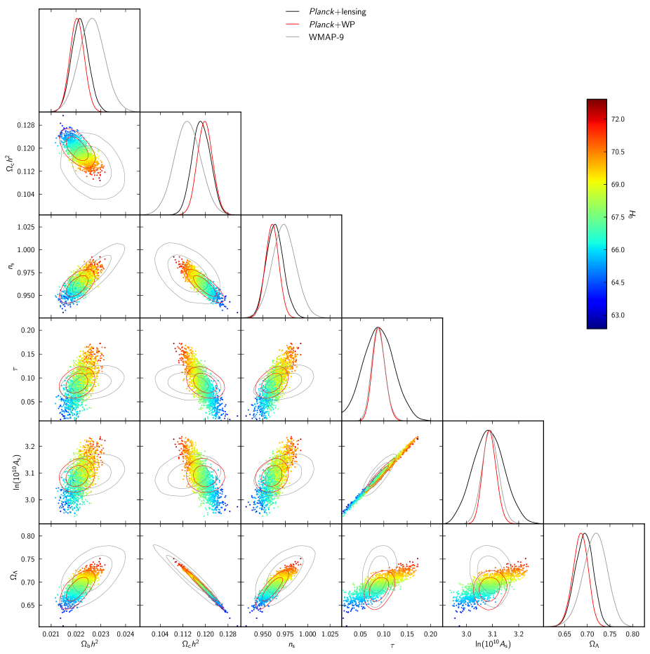
Table 2 summarizes our constraints on cosmological parameters from the Planck temperature power spectrum alone (labelled “Planck”), from Planck in combination with Planck lensing (Planck+lensing) and with WMAP low-$\ell$ polarization (Planck+WP). Figure 2 shows a selection of corresponding constraints on pairs of parameters and fully marginalized one-parameter constraints compared to the final results from WMAP (Bennett et al. 2012).

Table 2: Cosmological parameter values for the six-parameter base $\rm{\Lambda CDM}$ model. Columns 2 and 3 give results for the Planck temperature power spectrum data alone. Columns 4 and 5 combine the Planck temperature data with Planck lensing, and columns 6 and 7 include WMAP polarization at low multipoles. We give best fit parameters (i.e. the parameters that maximise the overall likelihood for each data combination) as well as $68\%$ confidence limits for constrained parameters. The first six parameters have flat priors. The remainder are derived parameters as discussed in Sect. 2. Beam, calibration parameters, and foreground parameters (see Sect. 4) are not listed for brevity. Constraints on foreground parameters for Planck+WP are given later in Table 5.

Planck Planck+lensing Planck+WP

Parameter Best fit 68% limits Best fit 68% limits Best fit 68% limits

$$\Omega_{\mathrm{b}}h^{2}$$.

.

.

.

.

.

.

.

.

.

.

.

.

.

.

.

.

.

.

.

.

.

.

.

.

.

3.1 Acoustic scale

The characteristic angular size of the fluctuations in the CMB is called the acoustic scale. It is determined by the comoving size of the sound horizon at the time of last-scattering, $r_{\rm s}(z_{\ast})$, and the angular diameter distance at which we are observing the fluctuations, $D_{\rm A}(z_{\ast})$. With accurate measurement of seven acoustic peaks, Planck determines the observed angular size $\theta_{\ast}=r_{\rm s}/D_{\rm A}$ to better than $0.1\%$ precision at $1\thinspace\sigma$:

$$\theta_{\ast}=(1.04148\pm 0.00066)\times 10^{-2}=0.596724^{\circ}\pm 0.00038^{\circ}.$$ (10)

Since this parameter is constrained by the positions of the peaks but not their amplitudes, it is quite robust; the measurement is very stable to changes in data combinations and the assumed cosmology. Foregrounds, beam uncertainties, or any systematic effects which only contribute a smooth component to the observed spectrum will not substantially affect the frequency of the oscillations, and hence this determination is likely to be Planck’s most robust precision measurement. The situation is analogous to baryon acoustic oscillations measurements in large-scale structure surveys (see Sect. 5.2), but the CMB acoustic measurement has the advantage that it is based on observations of the Universe when the fluctuations were very accurately linear, so second and higher-order effects are expected to be negligible.

The tight constraint on $\theta_{\ast}$ also implies tight constraints on some combinations of the cosmological parameters that determine $D_{\rm A}$ and $r_{\rm s}$. The sound horizon $r_{\rm s}$ depends on the physical matter density parameters, and $D_{\rm A}$ depends on the late-time evolution and geometry. Parameter combinations that fit the Planck data must be constrained to be close to a surface of constant $\theta_{\ast}$. This surface depends on the model that is assumed. For the base $\rm{\Lambda CDM}$ model, the main parameter dependence is approximately described by a $0.3\%$ constraint in the three-dimensional $\Omega_{\mathrm{m}}$–$h$–$\Omega_{\mathrm{b}}h^{2}$ subspace:

$$\Omega_{\mathrm{m}}h^{3.2}(\Omega_{\mathrm{b}}h^{2})^{-0.54}=0.695\pm 0.002\quad\mbox{(68\%; {Planck})}.$$ (11)

Reducing further to a two-dimensional subspace gives a $0.6\%$ constraint on the combination

$$\Omega_{\mathrm{m}}h^{3}=0.0959\pm 0.0006\quad\mbox{(68\%; {Planck})}.$$ (12)

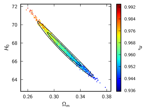
The principle component analysis direction is actually $\Omega_{\mathrm{m}}h^{2.93}$ but this is conveniently close to $\Omega_{\mathrm{m}}h^{3}$ and gives a similar constraint. The simple form is a coincidence of the $\rm{\Lambda CDM}$ cosmology, error model, and particular parameter values of the model (Percival et al. 2002; Howlett et al. 2012). The degeneracy between $H_{0}$ and $\Omega_{\mathrm{m}}$ is illustrated in Fig. 3: parameters are constrained to lie in a narrow strip where $\Omega_{\mathrm{m}}h^{3}$ is nearly constant, but the orthogonal direction is much more poorly constrained. The degeneracy direction involves consistent changes in the $H_{0}$, $\Omega_{\mathrm{m}}$, and $\Omega_{\mathrm{b}}h^{2}$ parameters, so that the ratio of the sound horizon and angular diameter distance remains nearly constant. Changes in the density parameters, however, also have other effects on the power spectrum and the spectral index $n_{\rm s}$ also changes to compensate. The degeneracy is not exact; its extent is much more sensitive to other details of the power spectrum shape. Additional data can help further to restrict the degeneracy. Figure 3 shows that adding WMAP polarization has almost no effect on the $\Omega_{\mathrm{m}}h^{3}$ measurement, but shrinks the orthogonal direction slightly from $\Omega_{\mathrm{m}}h^{-3}=1.03\pm 0.13$ to $\Omega_{\mathrm{m}}h^{-3}=1.04\pm 0.11$.

Figure 3: Constraints in the $\Omega_{\rm m}$–$H_{0}$ plane. Points show samples from the Planck-only posterior, coloured by the corresponding value of the spectral index $n_{\rm s}$. The contours (68% and 95%) show the improved constraint from Planck+lensing+WP. The degeneracy direction is significantly shortened by including WP, but the well-constrained direction of constant $\Omega_{\mathrm{m}}h^{3}$ (set by the acoustic scale), is determined almost equally accurately from Planck alone.

3.2 Hubble parameter and dark energy density

The Hubble constant, $H_{0}$, and matter density parameter, $\Omega_{\mathrm{m}}$, are only tightly constrained in the combination $\Omega_{\mathrm{m}}h^{3}$ discussed above, but the extent of the degeneracy is limited by the effect of $\Omega_{\mathrm{m}}h^{2}$ on the relative heights of the acoustic peaks. The projection of the constraint ellipse shown in Fig. 3 onto the axes therefore yields useful marginalized constraints on $H_{0}$ and $\Omega_{\mathrm{m}}$ (or equivalently $\Omega_{\Lambda}$) separately. We find the $2\%$ constraint on $H_{0}$:

$$H_{0}=(67.4\pm 1.4)\thinspace{\rm km}\thinspace{\rm s}^{-1}\thinspace{\rm Mpc}^{-1}\quad\mbox{(68\%; {Planck})}.$$ (13)

The corresponding constraint on the dark energy density parameter is

$$\Omega_{\Lambda}=0.686\pm 0.020\quad\mbox{(68\%; {Planck})},$$ (14)

and for the physical matter density we find

$$\Omega_{\mathrm{m}}h^{2}=0.1423\pm 0.0029\quad\mbox{(68\%; {Planck})}.$$ (15)

Note that these indirect constraints are highly model dependent. The data only measure accurately the acoustic scale, and the relation to underlying expansion parameters (e.g., via the angular-diameter distance) depends on the assumed cosmology, including the shape of the primordial fluctuation spectrum. Even small changes in model assumptions can change $H_{0}$ noticeably; for example, if we neglect the $0.06\thinspace\text{eV}$ neutrino mass expected in the minimal hierarchy, and instead take $\sum m_{\nu}=0$, the Hubble parameter constraint shifts to

$$H_{0}=(68.0\pm 1.4)\thinspace{\rm km}\thinspace{\rm s}^{-1}\thinspace{\rm Mpc}^{-1}\thinspace\thinspace\thinspace\mbox{(68\%; {Planck}, $\sum m_{\nu}=0$)}.$$ (16)

3.3 Matter densities

Planck can measure the matter densities in baryons and dark matter from the relative heights of the acoustic peaks. However, as discussed above, there is a partial degeneracy with the spectral index and other parameters that limits the precision of the determination. With Planck there are now enough well measured peaks that the extent of the degeneracy is limited, giving $\Omega_{\mathrm{b}}h^{2}$ to an accuracy of $1.5\%$ without any additional data:

$$\Omega_{\mathrm{b}}h^{2}=0.02207\pm 0.00033\quad\mbox{(68\%; {Planck})}.$$ (17)

Adding WMAP polarization information shrinks the errors by only $10\%$.

The dark matter density is slightly less accurately measured at around 3%:

$$\Omega_{\mathrm{c}}h^{2}=0.1196\pm 0.0031\quad\mbox{(68\%; {Planck})}.$$ (18)

3.4 Optical depth

Figure 4: Marginalized constraints on parameters of the base $\rm{\Lambda CDM}$ model for various data combinations.

Small-scale fluctuations in the CMB are damped by Thomson scattering from free electrons produced at reionization. This scattering suppresses the amplitude of the acoustic peaks by $e^{-2\tau}$ on scales that correspond to perturbation modes with wavelength smaller than the Hubble radius at reionization. Planck measures the small-scale power spectrum with high precision, and hence accurately constrains the damped amplitude $e^{-2\tau}A_{\rm s}$. With only unlensed temperature power spectrum data, there is a large degeneracy between $\tau$ and $A_{\rm s}$, which is weakly broken only by the power in large-scale modes that were still super-Hubble scale at reionization. However, lensing depends on the actual amplitude of the matter fluctuations along the line of sight. Planck accurately measures many acoustic peaks in the lensed temperature power spectrum, where the amount of lensing smoothing depends on the fluctuation amplitude. Furthermore Planck’s lensing potential reconstruction provides a more direct measurement of the amplitude, independently of the optical depth. The combination of the temperature data and Planck’s lensing reconstruction can therefore determine the optical depth $\tau$ relatively well. The combination gives

$$\tau=0.089\pm 0.032\quad\mbox{(68\%; {Planck}+lensing)}.$$ (19)

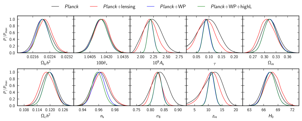
As shown in Fig. 4 this provides marginal confirmation (just under $2\thinspace\sigma$) that the total optical depth is significantly higher than would be obtained from sudden reionization at $z\sim 6$, and is consistent with the WMAP-9 constraint, $\tau=0.089\pm 0.014$, from large-scale polarization (Bennett et al. 2012). The large-scale $E$-mode polarization measurement is very challenging because it is a small signal relative to polarized Galactic emission on large scales, so this Planck polarization-free result is a valuable cross-check. The posterior for the Planck temperature power spectrum measurement alone also consistently peaks at $\tau\sim 0.1$, where the constraint on the optical depth is coming from the amplitude of the lensing smoothing effect and (to a lesser extent) the relative power between small and large scales.

Since lensing constrains the underlying fluctuation amplitude, the matter density perturbation power is also well determined:

$$\sigma_{8}=0.823\pm 0.018\quad\mbox{(68\%; {Planck}+lensing)}.$$ (20)

Much of the residual uncertainty is caused by the degeneracy with the optical depth. Since the small-scale temperature power spectrum more directly fixes $\sigma_{8}e^{-\tau}$, this combination is tightly constrained:

$$\sigma_{8}e^{-\tau}=0.753\pm 0.011\quad\mbox{(68\%; {Planck}+lensing)}.$$ (21)

The estimate of $\sigma_{8}$ is significantly improved to $\sigma_{8}=0.829\pm 0.012$ by using the WMAP polarization data to constrain the optical depth, and is not strongly degenerate with $\Omega_{\mathrm{m}}$. (We shall see in Sect. 5.5 that the Planck results are discrepant with recent estimates of combinations of $\sigma_{8}$ and $\Omega_{\mathrm{m}}$ from cosmic shear measurements and counts of rich clusters of galaxies.)

3.5 Spectral index

The scalar spectral index defined in Eq. (2) is measured by Planck data alone to 1% accuracy:

$$n_{\rm s}=0.9616\pm 0.0094\quad\mbox{(68\%; {Planck})}.$$ (22)

Since the optical depth $\tau$ affects the relative power between large scales (that are unaffected by scattering at reionization) and intermediate and small scales (that have their power suppressed by $e^{-2\tau}$), there is a partial degeneracy with $n_{\rm s}$. Breaking the degeneracy between $\tau$ and $n_{s}$ using WMAP polarization leads to a small improvement in the constraint:

$$n_{\rm s}=0.9603\pm 0.0073\quad\mbox{(68\%; {Planck}+WP)}.$$ (23)

Comparing Eqs. (22) and (23), it is evident that the Planck temperature spectrum spans a wide enough range of multipoles to give a highly significant detection of a deviation of the scalar spectral index from exact scale invariance (at least in the base $\Lambda$CDM cosmology) independent of WMAP polarization information.

One might worry that the spectral index parameter is degenerate with foreground parameters, since these act to increase smoothly the amplitudes of the temperature power spectra at high multipoles. The spectral index is therefore liable to potential systematic errors if the foreground model is poorly constrained. Figure 4 shows the marginalized constraints on the $\rm{\Lambda CDM}$ parameters for various combinations of data, including adding high-resolution CMB measurements. As will be discussed in Sect. 4, the use of high-resolution CMB provides tighter constraints on the foreground parameters (particularly “minor” foreground components) than from Planck data alone. However, the small shifts in the means and widths of the distributions shown in Fig. 4 indicate that, for the base $\Lambda$CDM cosmology, the errors on the cosmological parameters are not limited by foreground uncertainties when considering Planck alone. The effects of foreground modelling assumptions and likelihood choices on constraints on $n_{\rm s}$ are discussed in Appendix C.

4 Planck combined with high-resolution CMB experiments: the base $\Lambda$CDM model

Table 3: Summary of the CMB temperature data sets used in this analysis.

      Frequency       Area       $$\ell_{\rm min} \ell_{\rm max} S_{\rm cut}^{\mbox{\scriptsize{\it a}}} \nu_{\rm CMB} \nu_{\rm tSZ} \nu_{\rm Radio} \nu_{\rm IR} \ldots \ldots \ldots \ldots \ldots \ldots \ldots \ldots$$                                           Experiment       [GHz]       [deg²]       [mJy]       [GHz]       [GHz]       [GHz]       [GHz] Planck.       100       23846       50       1200              100.0       103.1               Planck.       143       15378       50       2000              143.0       145.1              146.3 Planck.       217       15378       500       2500              217.0                     225.7 ACT (D13).       148       600       540       9440       15.0       148.4       146.9       147.6       149.7 ACT (D13).       218       600       1540       9440       15.0       218.3       220.2       217.6       219.6 SPT-high (R12).       95       800       2000       10000       6.4       95.0       97.6       95.3       97.9 SPT-high (R12).       150       800       2000       10000       6.4       150.0       152.9       150.2       153.8 SPT-high (R12).       220       800       2000       10000       6.4       220.0       218.1       214.1       219.6

$${}^{\textit{a}}$$Flux-density cut applied to the map by the point-source mask. For Planck the point-source mask is based on a composite of sources identified in the 100–353 GHz maps, so there is no simple flux cut.

The previous section adopted a foreground model with relatively loose priors on its parameters. As discussed there and in Planck Collaboration XV (2014), for the base $\Lambda$CDM model, the cosmological parameters are relatively weakly correlated with the parameters of the foreground model and so we expect that the cosmological results reported in Sect. 3 are robust. Fortunately, we can get an additional handle on unresolved foregrounds, particularly “minor” components such as the kinetic SZ effect, by combining the Planck data with data from high-resolution CMB experiments. The consistency of results obtained with Planck data alone and Planck data combined with high-resolution CMB data gives added confidence to our cosmological results, particularly when we come to investigate extensions to the base $\Lambda$CDM cosmology (Sect. 6). In this section, we review the high-resolution CMB data (hereafter, usually denoted highL) that we combine with Planck and then discuss how the foreground model is adapted (with additional “nuisance” parameters) to handle multiple CMB data sets. We then discuss the results of an MCMC analysis of the base $\Lambda$CDM model combining Planck data with the high-$\ell$ data.

4.1 Overview of the high-$\ell$ CMB data sets

The Atacama Cosmology Telescope (ACT) mapped the sky from 2007 to 2010 in two distinct regions, the equatorial stripe (ACTe) along the celestial equator, and the southern stripe (ACTs) along declination $-55^{\circ}$, observing in total about $600\thinspace\mathrm{deg}^{2}$. The ACT data sets at $148$ and $218\thinspace\mathrm{GHz}$ are presented in Das et al. (2013, hereafter D13) and cover the angular scales $540<\ell<9440$ at $148\thinspace\mathrm{GHz}$ and $1540<\ell<9440$ at $218\thinspace\mathrm{GHz}$. Beam errors are included in the released covariance matrix. We include the ACT $148\times 148$ spectra for $\ell\geq 1000$, and the ACT $148\times 218$ and $218\times 218$ spectra for $\ell\geq 1500$. The inclusion of ACT spectra to $\ell=1000$ improves the accuracy of the inter-calibration parameters between the high-$\ell$ experiments and Planck.

The South Pole Telescope observed a region of sky over the period 2007–10. Spectra are reported in Keisler et al. (2011, hereafter K11) and Story et al. (2012, hereafter S12) for angular scales $650<\ell<3000$ at $150\thinspace\mathrm{GHz}$, and in Reichardt et al. (2012, hereafter R12) for angular scales $2000<\ell<10000$ at 95, 150 and $220\thinspace\mathrm{GHz}$. Beam errors are included in the released covariance matrices used to form the SPT likelihood. The parameters of the base $\Lambda$CDM cosmology derived from the WMAP-7+S12 data and (to a lesser extent) from K11 are in tension with Planck. Since the S12 spectra have provided the strongest CMB constraints on cosmological parameters prior to Planck, this discrepancy merits a more detailed analysis, which is presented in appendix B. The S12 and K11 data are not used in combination with Planck in this paper. Since the primary purpose of including high-$\ell$ CMB data is to provide stronger constraints on foregrounds, we use only the R12 SPT data at $\ell>2000$ in combination with Planck. We ignore any correlations between ACT/SPT and Planck spectra over the overlapping multipole ranges.

Table 3 summarizes some key features of the CMB data sets used in this paper.

Figure 5: Top: Planck spectra at $100$, $143$ and $217\thinspace\mathrm{GHz}$ without subtraction of foregrounds. Middle: SPT spectra from R12 at 95, 150 and $220\thinspace\mathrm{GHz}$, recalibrated to Planck using the best-fit calibration, as discussed in the text. The S12 SPT spectrum at $150\thinspace\mathrm{GHz}$ is also shown, but without any calibration correction. This spectrum is discussed in detail in Appendix B, but is not used elsewhere in this paper. Bottom: ACT spectra (weighted averages of the equatorial and southern fields) from D13 at $148$ and $220\thinspace\mathrm{GHz}$, and the $148\times 220\thinspace\mathrm{GHz}$ cross-spectrum, with no extragalactic foreground corrections, recalibrated to the Planck spectra as discussed in the text. The solid line in each panel shows the best-fit base $\Lambda$CDM model from the combined Planck+WP+highL fits listed in Table 5.

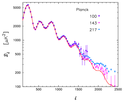
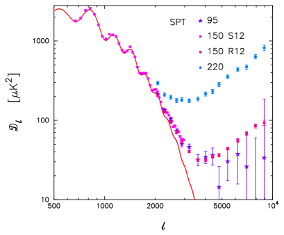
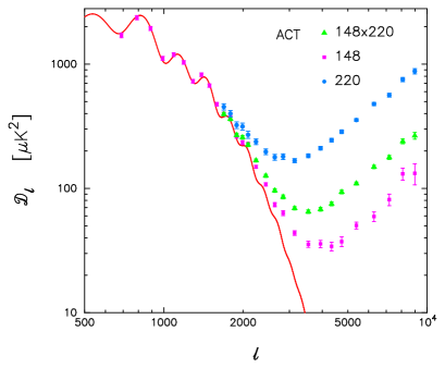
4.2 Model of unresolved foregrounds and “nuisance” parameters

The model for unresolved foregrounds used in the Planck likelihood is described in detail in Planck Collaboration XV (2014). Briefly, the model includes power spectrum templates for clustered extragalactic point sources (the cosmic infra-red background, hereafter CIB), thermal (tSZ) and kinetic (kSZ) Sunyaev-Zeldovich contributions, and the cross-correlation (tSZ$\times$CIB) between infra-red galaxies and the thermal Sunyaev-Zeldovich effect. The model also includes amplitudes for the Poisson contributions from radio and infra-red galaxies. The templates are described in Planck Collaboration XV (2014) and are kept fixed here. (Appendix C discusses briefly a few tests showing the impact of varying some aspects of the foreground model.) The model for unresolved foregrounds is similar to the models developed by the ACT and the SPT teams (e.g., R12; Dunkley et al. 2013). The main difference is in the treatment of the Poisson contribution from radio and infra-red galaxies. In the ACT and SPT analyses, spectral models are assumed for radio and infra-red galaxies. The Poisson point source contributions can then be described by an amplitude for each population, assuming either fixed spectral parameters or solving for them. In addition, one can add additional parameters to describe the decorrelation of the point source amplitudes with frequency (see e.g., Millea et al. 2012). The Planck model assumes free amplitudes for the point sources at each frequency, together with appropriate correlation coefficients between frequencies. The model is adapted to handle the ACT and SPT data as discussed later in this section.

Figure 5 illustrates the importance of unresolved foregrounds in interpreting the power spectra of the three CMB data sets. The upper panel of Fig. 5 shows the Planck temperature spectra at $100$, $143$, and $217\thinspace\mathrm{GHz}$, without corrections for unresolved foregrounds (to avoid overcrowding, we have not plotted the $143\times 217$ spectrum). The solid (red) lines show the best-fit base $\Lambda$CDM CMB spectrum corresponding to the combined Planck+ACT+SPT+WMAP polarization likelihood analysis, with parameters listed in Table 5. The middle panel shows the SPT spectra at $95$, $150$ and $220\thinspace\mathrm{GHz}$ from S12 and R12. In this figure, we have recalibrated the R12 power spectra to match Planck using calibration parameters derived from a full likelihood analysis of the base $\Lambda$CDM model. The S12 spectrum plotted is exactly as tabulated in S12, i.e., we have not recalibrated this spectrum to Planck. (The consistency of the S12 spectrum with the theoretical model is discussed in further detail in Appendix B.) The lower panel of Fig. 5 shows the ACT spectra from D13, recalibrated to Planck with calibration coefficients determined from a joint likelihood analysis. The power spectra plotted are an average of the ACTe and ACTs spectra, and include the small Galactic dust corrections described in D13.

The small-scale SPT (R12) and ACT (D13) data are dominated by the extragalactic foregrounds and hence are highly effective in constraining the multi-parameter foreground model. In contrast, Planck has limited angular resolution and therefore limited ability to constrain unresolved foregrounds. Planck is sensitive to the Poisson point source contribution at each frequency and to the CIB contribution at $217\thinspace\mathrm{GHz}$. Planck has some limited sensitivity to the tSZ amplitude from the $100\thinspace\mathrm{GHz}$ channel (and almost no sensitivity at $143\thinspace\mathrm{GHz}$). The remaining foreground contributions are poorly constrained by Planck and highly degenerate with each other in a Planck-alone analysis. The main gain in combining Planck with the high-resolution ACT and SPT data is in breaking some of the degeneracies between foreground parameters which are poorly determined from Planck data alone.

An important extension of the foreground parameterization described here over that developed in Planck Collaboration XV (2014) concerns the use of effective frequencies. Different experiments (and different detectors within a frequency band) have non-identical bandpasses (Planck Collaboration IX 2014) and this needs to be taken into account in the foreground modelling. Consider, for example, the amplitude of the CIB template at $217\thinspace\mathrm{GHz}$, $A^{\rm CIB}_{217}$, introduced in Planck Collaboration XV (2014). The effective frequency for a dust-like component for the averaged $217\thinspace\mathrm{GHz}$ spectrum used in the Planck likelihood is $225.7\thinspace\mathrm{GHz}$. To avoid cumbersome notation, we solve for the CIB amplitude $A^{\rm CIB}_{217}$ at the CMB effective frequency of $217\thinspace\mathrm{GHz}$. The actual amplitude measured in the Planck $217\thinspace\mathrm{GHz}$ band is $1.33A^{\rm CIB}_{217}$, reflecting the different effective frequencies of a dust-like component compared to the blackbody primordial CMB (see Eq. 30 below). With appropriate effective frequencies, the single amplitude $A^{\rm CIB}_{217}$ can be used to parameterize the CIB contributions to the ACT and SPT power spectra in their respective $218$ and $220\thinspace\mathrm{GHz}$ bands. A similar methodology is applied to match the tSZ amplitudes for each experiment.

The relevant effective frequencies for the foreground parameterization discussed below are listed in Table 3. For the high resolution experiments, these are as quoted in R12 and Dunkley et al. (2013). For Planck these effective frequencies were computed from the individual HFI bandpass measurements (Planck Collaboration IX 2014), and vary by a few percent from detector to detector. The numbers quoted in Table 3 are based on an approximate average of the individual detector bandpasses using the weighting scheme for individual detectors/detector-sets applied in the CamSpec likelihood. (The resulting bandpass correction factors for the tSZ and CIB amplitudes should be accurate to better than $5\%$.) Note that all temperatures in this section are in thermodynamic units.

The ingredients of the foreground model and associated “nuisance” parameters are summarized in the following paragraphs.

Calibration factors:

To combine the Planck, ACT and SPT likelihoods it is important to incorporate relative calibration factors, since the absolute calibrations of ACT and SPT have large errors (e.g., around $3.5\%$ in power for the SPT $150\thinspace\mathrm{GHz}$ channel). We introduce three map calibration parameters $y^{\rm SPT}_{95}$, $y^{\rm SPT}_{150}$ and $y^{\rm SPT}_{220}$ to rescale the R12 SPT spectra. These factors rescale the cross-spectra at frequencies $\nu_{i}$ and $\nu_{j}$ as

$$C_{\ell}^{\nu_{i}\times\nu_{j}}\rightarrow y_{\nu_{i}}^{{\rm SPT}}y_{\nu_{j}}^{{\rm SPT}}C_{\ell}^{\nu_{i}\times\nu_{j}}.$$ (24)

In the analysis of ACT, we solve for different map calibration factors for the ACTe and ACTs spectra, $y^{\mathrm{ACTe}}_{148}$, $y^{\mathrm{ACTs}}_{148}$, $y^{\mathrm{ACTe}}_{218}$, and $y^{\mathrm{ACTs}}_{218}$. In addition, we solve for the $100\times 100$ and $217\times 217$ Planck power-spectrum calibration factors $c_{100}$ and $c_{217}$, with priors as described in Planck Collaboration XV (2014); see also Table 4. (The use of map calibration factors for ACT and SPT follows the conventions adopted by the ACT and SPT teams, while for the Planck power spectrum analysis we have consistently used power-spectrum calibration factors.)

In a joint parameter analysis of Planck+ACT+SPT, the inclusion of these calibration parameters leads to recalibrations that match the ACT, SPT and Planck $100\thinspace\mathrm{GHz}$ and $217\thinspace\mathrm{GHz}$ channels to the calibration of the Planck $143\times 143$ spectrum (which, in turn, is linked to the calibration of the HFI 143-5 detector, as described in Planck Collaboration XV 2014). It is worth mentioning here that the Planck $143\times 143\thinspace\mathrm{GHz}$ spectrum is 2.5% lower than the WMAP-9 combined V+W power spectrum (Hinshaw et al. 2012). This calibration offset between Planck HFI channels and WMAP is discussed in more detail in  Planck Collaboration XXXI (2014) and in Appendix A.

Poisson point source amplitudes:

To avoid any possible biases in modelling a mixed population of sources (synchrotron+dusty galaxies) with differing spectra, we solve for each of the Poisson point source amplitudes as free parameters. Thus, for Planck we solve for $A^{\rm PS}_{100}$, $A^{\rm PS}_{143}$, and $A^{\rm PS}_{217}$, giving the amplitude of the Poisson point source contributions to ${\cal D}_{3000}$ for the $100\times 100$, $143\times 143$, and $217\times 217$ spectra. The units of $A^{\rm PS}_{\nu}$ are therefore $\mu{\rm K}^{2}$. The Poisson point source contribution to the $143\times 217$ spectrum is expressed as a correlation coefficient, $r^{\rm PS}_{143\times 217}$:

$${\cal D}^{143\times 217}_{3000}=r^{\rm PS}_{143\times 217}\sqrt{A^{\rm PS}_{143}A^{\rm PS}_{217}}.$$ (25)

Note that we do not use the Planck $100\times 143$ and $100\times 217$ spectra in the likelihood, and so we do not include correlation coefficients $r^{\rm PS}_{100\times 143}$ or $r^{\rm PS}_{100\times 217}$. (These spectra carry little additional information on the primordial CMB, but would require additional foreground parameters had we included them in the likelihood.)

In an analogous way, the point source amplitudes for ACT and SPT are characterized by the amplitudes $A^{\rm PS,ACT}_{148}$, $A^{\rm PS,ACT}_{217}$, $A^{\rm PS,SPT}_{95}$, $A^{\rm PS,SPT}_{150}$, and $A^{\rm PS,SPT}_{220}$ (all in units of $\mu{\rm K}^{2}$) and three correlation coefficients $r^{\rm PS}_{95\times 150}$, $r^{\rm PS}_{95\times 220}$, and $r^{\rm PS}_{150\times 220}$. The last of these correlation coefficients is common to ACT and SPT.

Kinetic SZ:

The kSZ template used here is from Trac et al. (2011). We solve for the amplitude $A^{\rm kSZ}$ (in units of $\mu{\rm K}^{2}$):

$${\cal D}^{\rm kSZ}_{\ell}=A^{\rm kSZ}{{\cal D}^{\rm kSZ\thinspace template}_{\ell}\over{\cal D}^{\rm kSZ\thinspace template}_{3000}}.$$ (26)

Thermal SZ:

We use the $\epsilon=0.5$ tSZ template from Efstathiou & Migliaccio (2012) normalized to a frequency of $143\thinspace$GHz.

For cross-spectra between frequencies $\nu_{i}$ and $\nu_{j}$, the tSZ template is normalized as

$${\cal D}_{\ell}^{\mathrm{tSZ}_{\nu_{i}\times\nu_{j}}}=A^{\rm tSZ}_{143}\frac{f(\nu_{i})f(\nu_{j})}{f^{2}(\nu_{0})}{{\cal D}_{\ell}^{\rm{tSZ\thinspace template}}\over{\cal D}_{3000}^{\rm{tSZ\thinspace template}}},$$ (27)

where $\nu_{0}$ is the reference frequency of $143\thinspace\mathrm{GHz}$, ${\cal D}_{\ell}^{\rm{tSZ\ template}}$ is the template spectrum at $143\thinspace\mathrm{GHz}$, and

$$f(\nu)=\left(x{e^{x}+1\over e^{x}-1}-4\right),\quad{\rm with}\ x={h\nu\over k_{\rm B}T_{\rm CMB}}.$$ (28)

The tSZ contribution is therefore characterized by the amplitude $A^{\rm tSZ}_{143}$ in units of $\mu{\rm K}^{2}$.

We neglect the tSZ contribution for any spectra involving the Planck $217\thinspace$GHz, ACT $218\thinspace$GHz, and SPT $220\thinspace$GHz channels, since the tSZ effect has a null point at $\nu=217\thinspace{\rm GHz}$. (For Planck the bandpasses of the $217\thinspace$GHz detectors see less than $0.1\%$ of the $143\thinspace$GHz tSZ power.)

Cosmic infrared background:

The CIB contributions are neglected in the Planck $100\thinspace$GHz and SPT $95\thinspace$GHz bands and in any cross-spectra involving these frequencies. The CIB power spectra at higher frequencies are characterized by three amplitude parameters and a spectral index,

$${\cal D}^{{\rm CIB}_{143\times 143}}_{\ell} = A^{\rm CIB}_{143}\left({\ell\over 3000}\right)^{\gamma^{\rm CIB}},$$ (29a)

$${\cal D}^{{\rm CIB}_{217\times 217}}_{\ell} = A^{\rm CIB}_{217}\left({\ell\over 3000}\right)^{\gamma^{\rm CIB}},$$ (29b)

$${\cal D}^{{\rm CIB}_{143\times 217}}_{\ell} = r^{\rm CIB}_{143\times 217}\sqrt{A^{\rm CIB}_{143}A^{\rm CIB}_{217}}\left({\ell\over 3000}\right)^{\gamma^{\rm CIB}},$$ (29c)

where $A^{\rm CIB}_{143}$ and $A^{\rm CIB}_{143}$ are expressed in $\mu{\rm K}^{2}$. As explained above, we define these amplitudes at the Planck CMB frequencies of $143$ and $217\thinspace$GHz and compute scalings to adjust these amplitudes to the effective frequencies for a dust-like spectrum for each experiment. The scalings are

$${\cal D}^{{\rm CIB}_{\nu_{i}\times\nu_{j}}}_{\ell}={\cal D}^{{\rm CIB}_{{\nu_{i0}\times\nu_{\!j0}}}}_{3000}\left({g(\nu_{i})g(\nu_{j})\over g(\nu_{i0})g(\nu_{j0})}\right)\left(\frac{\nu_{i}\nu_{j}}{\nu_{i0}\nu_{j0}}\right)^{\beta_{\rm d}}\frac{B_{\nu_{i}}(T_{\rm d})}{B_{\nu_{i0}}(T_{\rm d})}\frac{B_{\nu_{j}}(T_{\rm d})}{B_{\nu_{j0}}(T_{\rm d})},$$

(30)

where $B_{\nu}(T_{\rm d})$ is the Planck function at a frequency $\nu$,

$$g(\nu)=\left[\partial B_{\nu}(T)/\partial T\right]^{-1}|_{T_{\rm CMB}}$$ (31)

converts antenna temperature to thermodynamic temperature, $\nu_{i}$ and $\nu_{j}$ refer to the Planck/ACT/SPT dust effective frequencies, and $\nu_{i0}$ and $\nu_{j0}$ refer to the corresponding reference CMB Planck frequencies. In the analysis presented here, the parameters of the CIB spectrum are fixed to $\beta_{\rm d}=2.20$ and $T_{\rm d}=9.7\thinspace$K, as discussed in Addison et al. (2012a). The model of Eq. (30) then relates the Planck reference amplitudes of Eqs.  (29b–29c) to the neighbouring Planck, ACT, and SPT effective frequencies, assuming that the CIB is perfectly correlated over these small frequency ranges.

It has been common practice in recent CMB parameter studies to fix the slope of the CIB spectrum to $\gamma^{\rm CIB}=0.8$ (e.g., Story et al. 2012; Dunkley et al. 2013). In fact, the shape of the CIB spectrum is poorly constrained at frequencies below $353\thinspace$GHz and we have decided to reflect this uncertainty by allowing the slope $\gamma^{\rm CIB}$ to vary. We adopt a Gaussian prior on $\gamma^{\rm CIB}$ with a mean of $0.7$ and a dispersion of $0.2$. In reality, the CIB spectrum is likely to have some degree of curvature reflecting the transition between linear (two-halo) and non-linear (one-halo) clustering (see e.g., Cooray & Sheth 2002; Planck Collaboration XVIII 2011; Amblard et al. 2011; Thacker et al. 2012). However, a single power law is an adequate approximation within the restricted multipole range ($500\la\ell\la 3000$) over which the CIB contributes significantly to the Planck/ACT/SPT high-frequency spectra (as judged by the foreground-corrected power spectrum residuals shown in Figs. 7, 8 and 9 below). The prior on $\gamma^{\rm CIB}$ is motivated, in part, by the map-based Planck CIB analysis discussed in  Planck Collaboration XXX (2014) (see also Planck Collaboration XVIII 2014). Appendix C explores different parameterizations of the CIB power spectrum.

Table 4: Astrophysical parameters used to model foregrounds in our analysis, plus instrumental calibration and beam parameters. We include the symbol for each parameter, the prior range adopted for the MCMC analysis and a summary definition (see text for details). Square brackets denote hard priors, parentheses indicate Gaussian priors. Note that the beam eigenmode amplitudes require a correlation matrix to describe fully their joint prior, and that all but $\beta^{1}_{1}$ are internally marginalized over rather than sampled over for the main MCMC runs. The bottom two blocks are only used in the analysis including the ACT and SPT high-$\ell$ CMB data.

Parameter Prior range Definition $$A^{\mathrm{PS}}_{100} [0,360] \mathcal{D}^{100\times 100}_{3000} \mu\mathrm{K}^{2} A^{\mathrm{PS}}_{143} [0,270] A^{\mathrm{PS}}_{100} 143\thinspace A^{\mathrm{PS}}_{217} [0,450] A^{\mathrm{PS}}_{100} 217\thinspace r^{\mathrm{PS}}_{143\times 217} [0,1] 143 217\thinspace A^{\mathrm{CIB}}_{143} [0,20] \mathcal{D}^{143\times 143}_{3000} 143\thinspace \mu\mathrm{K}^{2} A^{\mathrm{CIB}}_{217} [0,80] A^{\mathrm{CIB}}_{143} 217\thinspace r^{\mathrm{CIB}}_{143\times 217} [0,1] 143 217\thinspace \gamma^{\mathrm{CIB}} [-2,2]\thinspace(0.7\pm 0.2) \mathcal{D}_{\ell}\propto\ell^{\gamma^{\mathrm{CIB}}} A^{\mathrm{tSZ}} [0,10] \mathcal{D}_{3000}^{143\times 143} 143\thinspace \mu\mathrm{K}^{2} A^{\mathrm{kSZ}} [0,10] \mathcal{D}_{3000} \mu\mathrm{K}^{2} \xi^{\mbox{\scriptsize{tSZ$\times$CIB}}} [0,1] c_{100} [0.98,1.02]\thinspace(1.0006\pm 0.0004) 100\thinspace 143\thinspace c_{217} [0.95,1.05]\thinspace(0.9966\pm 0.0015) 217\thinspace 143\thinspace \beta^{i}_{j} (0\pm 1) j j=1 i i=1 A^{\mathrm{PS},\thinspace\mathrm{ACT}}_{148} [0,30] \mathcal{D}^{148\times 148}_{3000} \mu\mathrm{K}^{2} A^{\mathrm{PS},\thinspace\mathrm{ACT}}_{218} [0,200] A^{\mathrm{PS},\thinspace\mathrm{ACT}}_{148} 218\thinspace r^{\mathrm{PS}}_{150\times 220} [0,1] 150 220\thinspace A^{\mathrm{ACTe}}_{\mathrm{dust}} [0,5]\thinspace(0.8\pm 0.2) \mathcal{D}_{3000} 150\thinspace \mu\mathrm{K}^{2} A^{\mathrm{ACTs}}_{\mathrm{dust}} [0,5]\thinspace(0.4\pm 0.2) A^{\mathrm{ACTe}}_{\mathrm{dust}} y^{\mathrm{ACTe}}_{148} [0.8,1.3] 148\thinspace 143\thinspace y^{\mathrm{ACTe}}_{217} [0.8,1.3] y^{\mathrm{ACTe}}_{148} 217\thinspace y^{\mathrm{ACTs}}_{148} [0.8,1.3] 148\thinspace 143\thinspace y^{\mathrm{ACTs}}_{217} [0.8,1.3] y^{\mathrm{ACTs}}_{148} 217\thinspace A^{\mathrm{PS},\thinspace\mathrm{SPT}}_{95} [0,30] \mathcal{D}^{95\times 95}_{3000} \mu\mathrm{K}^{2} A^{\mathrm{PS},\thinspace\mathrm{SPT}}_{150} [0,30] A^{\mathrm{PS},\thinspace\mathrm{SPT}}_{95} 150\thinspace A^{\mathrm{PS},\thinspace\mathrm{SPT}}_{220} [0,200] A^{\mathrm{PS},\thinspace\mathrm{SPT}}_{95} 220\thinspace r^{\mathrm{PS}}_{95\times 150} [0,1] 95 150\thinspace r^{\mathrm{PS}}_{95\times 220} [0,1] r^{\mathrm{PS}}_{95\times 150} 95 220\thinspace y^{\mathrm{SPT}}_{95} [0.8,1.3] 95\thinspace 143\thinspace y^{\mathrm{SPT}}_{150} [0.8,1.3] y^{\mathrm{SPT}}_{95} 150\thinspace y^{\mathrm{SPT}}_{220} [0.8,1.3] y^{\mathrm{SPT}}_{95} 220\thinspace$$. Contribution of Poisson point-source power to for Planck (in ) . As for , but at GHz . As for , but at GHz . Point-source correlation coefficient for Planck between and GHz . Contribution of CIB power to at the Planck CMB frequency for GHz (in ) . As for , but for GHz . CIB correlation coefficient between and GHz . Spectral index of the CIB angular power () . Contribution of tSZ to at GHz (in ) . Contribution of kSZ to (in ) . Correlation coefficient between the CIB and tSZ (see text) . Relative power spectrum calibration for Planck between GHz and GHz . Relative power spectrum calibration for Planck between GHz and GHz . Amplitude of the th beam eigenmode (–5) for the th cross-spectrum (–4) . Contribution of Poisson point-source power to for ACT (in ) . As for , but at GHz . Point-source correlation coefficient between and GHz (for ACT and SPT) . Contribution from Galactic cirrus to at GHz for ACTe (in ) . As , but for ACTs . Map-level calibration of ACTe at GHz relative to Planck GHz . As , but at GHz . Map-level calibration of ACTs at GHz relative to Planck GHz . As , but at GHz . Contribution of Poisson point-source power to for SPT (in ) . As for , but at GHz . As for , but at GHz . Point-source correlation coefficient between and GHz for SPT . As , but between and GHz . Map-level calibration of SPT at GHz relative to Planck GHz . As for , but at GHz . As for , but at GHz

Thermal-SZ/CIB cross-correlation:

The cross-correlation between dust emission from CIB galaxies and SZ emission from clusters (tSZ$\times$CIB) is expected to be non-zero. Because of uncertainties in the modelling of the CIB, it is difficult to compute this correlation with a high degree of precision. Addison et al. (2012b) present a halo-model approach to model this term and conclude that anti-correlations of around 10–20% are plausible between the clustered CIB components and the SZ at $150$ GHz. The tSZ$\times$CIB correlation is therefore expected to make a minor contribution to the unresolved foreground emission, but it is nevertheless worth including to determine how it might interact with other sub-dominant components, in particular the kSZ contribution. We use the Addison et al. (2012b) template spectrum in this paper and model the frequency dependence of the power spectrum as follows:

$${\cal D}_{\ell}^{{\mbox{\scriptsize{tSZ$\times$CIB}}}_{\nu_{i}\times\nu_{j}}} = -\xi^{{\mbox{\scriptsize{tSZ$\times$CIB}}}}{\cal D}_{\ell}^{{\mbox{\scriptsize{tSZ$\times$CIB}}}\thinspace\mathrm{template}}$$ (32)

$$\times\left(\sqrt{{\cal D}^{{\rm CIB}_{\nu_{i}\times\nu_{i}}}_{3000}{\cal D}^{{\rm tSZ}_{\nu_{j}\times\nu_{j}}}_{3000}}+\sqrt{{\cal D}^{{\rm CIB}_{\nu_{j}\times\nu_{j}}}_{3000}{\cal D}^{{\rm tSZ}_{\nu_{i}\times\nu_{i}}}_{3000}}\right),$$

where ${\cal D}_{\ell}^{{\mbox{\scriptsize{tSZ$\times$CIB}}}\thinspace\mathrm{template}}$ is the Addison et al. (2012b) template spectrum normalized to unity at $\ell=3000$ and ${\cal D}_{\ell}^{{\rm CIB}_{\nu_{i}\times\nu_{i}}}$ and ${\cal D}_{\ell}^{{\rm tSZ}_{\nu_{i}\times\nu_{i}}}$ are given by Eqs. (27) and (31). The tSZ$\times$CIB contribution is therefore characterized by the dimensionless cross-correlation coefficient $\xi^{{\mbox{\scriptsize{tSZ$\times$CIB}}}}$. With the definition of Eq. (32), a positive value of $\xi^{{\mbox{\scriptsize{tSZ$\times$CIB}}}}$ corresponds to an anti-correlation between the CIB and the tSZ signals.

Galactic dust:

For the masks used in the Planck CamSpec likelihood, Galactic dust makes a small contribution to ${\cal D}_{3000}$ of around $5\thinspace{\mu}{\rm K}^{2}$ to the $217\times 217$ power spectrum, $1.5\thinspace{\mu}{\rm K}^{2}$ to the $143\times 217$ spectrum, and around $0.5\thinspace{\mu}{\rm K}^{2}$ to the $143\times 143$ spectrum. We subtract the Galactic dust contributions from these power spectra using a “universal” dust template spectrum (at high multipoles this is accurately represented by a power law $\mathcal{D}^{\rm dust}_{\ell}\propto\ell^{-0.6}$). The template spectrum is based on an analysis of the $857\thinspace$GHz Planck maps described in  Planck Collaboration XV (2014), which uses mask-differenced power spectra to separate Galactic dust from an isotropic extragalactic CIB contribution. This Galactic dust correction is kept fixed with an amplitude determined by template fitting the $217$ and $143\thinspace$GHz Planck maps to the $857\thinspace$GHz map, as described in  Planck Collaboration XV (2014). Galactic dust contamination is ignored in the $100\times 100$ spectrum. The Galactic dust template spectrum is actually a good fit to the dust contamination at low multipoles, $\ell\ll 1000$; however, we limit the effects of any inaccuracies in dust subtraction at low multipoles by truncating the $217\times 217$ and $143\times 217$ spectra at a minimum multipole of $\ell_{\rm min}=500$. (At multipoles $\ell\la 1000$, the Planck temperature power spectra are signal dominated, so the $100\times 100$ and $143\times 143$ spectra contain essentially all of the information on cosmology.)

Figure 6: Comparison of the posterior distributions of the foreground parameters for Planck+WP (red) and Planck+WP+highL (black).

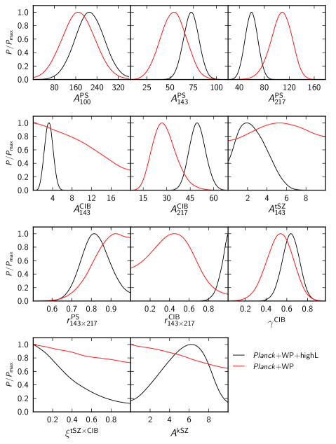
Compared to the contribution of Poisson point sources and the CIB, Galactic dust is a minor foreground component at $217\thinspace$GHz within our default mask, which retains 37% of the sky. However, the contribution of Galactic dust emission rises rapidly as more sky area is used. Extending the sky mask to $65\%$ of the sky (Planck Collaboration XV 2014, using the sequence of masks described in [), Galactic dust contributes to ${\cal D}_{3000}$ around $50\thinspace\mu{\rm K}^{2}$ at $217\thinspace$GHz (rising to around $200\thinspace\mu{\rm K}^{2}$ on the scale of the first acoustic peak) and becomes a major foreground component, with an amplitude close to the net contribution of Poisson point sources and the clustered CIB. There is therefore a trade-off between limiting the signal-to-noise at $143$ and $217\thinspace$GHz, by restricting the sky area, and potential systematic errors associated with modelling Galactic dust over a large area of sky (i.e., sensitivity to the assumption of a “universal” dust template spectrum). We have chosen to be conservative in this first cosmological analysis of Planck by limiting the sky area at $143$ and $217\thinspace\mathrm{GHz}$ so that dust contamination is a minor foreground at high multipoles. As a further test of the importance of Galactic dust, we have analysed a Planck likelihood that retains only $24.7\%$ of the sky (see Planck Collaboration XV 2014) at $217\thinspace$GHz. Within this mask the CIB dominates over Galactic dust at multipoles $\ell\ga 500$. There is a signal-to-noise penalty in using such a small area of sky at $217\thinspace$GHz, but otherwise the results from this likelihood are in good agreement with the results presented here. With the conservative choices adopted in this paper, Galactic dust has no significant impact on our cosmological results.

We follow R12 and subtract a small-scale dust contribution of ${\cal D}_{\ell}^{\rm dust}=2.19\thinspace\mu\mathrm{K}^{2}(\ell/3000)^{-1.2}$ from the R12 $220\thinspace$GHz spectrum. This correction was determined by cross-correlating the SPT data with model 8 of Finkbeiner et al. (1999). For the ACT data we marginalize over a residual Galactic dust component ${\cal D}^{\rm dust}_{\ell}=A^{\mathrm{ACTe/s}}_{\mathrm{dust}}(\ell/3000)^{-0.7}$, with different amplitudes for the southern and equatorial spectra, imposing Gaussian priors and frequency scaling as described in Dunkley et al. (2013).

Notice that the spectral index of the SPT dust correction is significantly steeper than the dust correction applied to the Planck spectra. In future analyses it would be useful to derive more accurate dust corrections for the high-resolution CMB data by cross-correlating the SPT and ACT maps with the Planck 545 and $857\thinspace$GHz maps. Since the dust corrections are relatively small for the high-resolution data used here, we adopt the correction described above in this paper.

In application of the likelihood to Planck data alone, the model for unresolved foregrounds and relative calibrations contains 13 parameters. In addition, we can solve for up to 20 beam eigenmode amplitudes (five amplitudes for each of the four spectra used in the Planck likelihood; see  Planck Collaboration XV 2014). In practice, we find that (usually) only the first beam eigenmode for the $100\times 100$ spectrum, $\beta^{1}_{1}$, has a posterior distribution that differs perceptibly from the prior, and we obtain nearly identical results on both foreground and cosmological parameters if we treat only the amplitude of this eigenmode as a parameter and analytically marginalize over the rest. This is the default adopted in this paper. (The analytic marginalization improves stability of the minimisation for best-fit searches, and makes the Planck likelihood less cumbersome for the user.)

The addition of ACT and SPT data introduces 17 extra parameters. We provide a summary of the 50 foreground and nuisance parameters in Table 4, including the prior ranges adopted in our MCMC analysis. The choice of priors for many of these parameters is, to a large extent, subjective. They were chosen at an early stage in the Planck analysis to reflect “theoretically plausible” allowed ranges of the foreground parameters and to be broad compared to the results from high-resolution CMB experiments (which evolved over the course of this analysis as results from more ACT and SPT data were published). The foreground parameters from ACT and SPT depend on the assumptions of the underlying cosmology, and hence it is possible to introduce biases in the solutions for extensions to the base $\Lambda$CDM cosmology if overly restrictive foreground priors are imposed on the Planck data. Using the priors summarized in Table 4, the consistency between the Planck-alone results and the solutions for Planck combined with ACT and SPT provides a crude (but informative) measure of the sensitivity of cosmological results on the foreground model. Appendix C discusses the effects on extended $\Lambda$CDM models of varying the priors on minor foreground components.

4.3 The base $\Lambda$CDM model

Table 5: Best-fit values and $68\%$ confidence limits for the base $\Lambda$CDM model. Beam and calibration parameters, and additional nuisance parameters for “highL” data sets are not listed for brevity but may be found in the Explanatory Supplement (Planck Collaboration 2013b).

Planck+WP Planck+WP+highL Planck+lensing+WP+highL Planck+WP+highL+BAO

Parameter Best fit 68% limits Best fit 68% limits Best fit 68% limits Best fit 68% limits

$$\Omega_{\mathrm{b}}h^{2}$$.

.

.

.

.

.

.

.

.

.

.

.

.

.

.

.

.

.

.

.

.

.

.

.

Cosmological and foreground parameters for the base six-parameter $\Lambda$CDM model are listed in Table 5, which gives best-fit values and 68% confidence limits. The first two columns list the parameters derived from the Planck+WP analysis discussed in Sect. 3, and are repeated here for easy reference. The next two columns list the results of combining the Planck+WP likelihoods with the ACT and SPT likelihoods following the model described above. We refer to this combination as “Planck+WP+highL” in this paper. The remaining columns list the parameter constraints combining the Planck+WP+highL likelihood with the Planck lensing and BAO likelihoods (see Sect. 5). Table 5 lists the cosmological parameters for the base $\Lambda$CDM model and a selection of derived cosmological parameters. These parameters are remarkably stable for such data combinations. We also list the values of the parameters describing the Planck foregrounds. A full list of all parameter values, including nuisance parameters, is given in the Explanatory Supplement (Planck Collaboration 2013b).

A comparison of the foreground parameter constraints from Planck+WP and Planck+WP+highL is shown in Fig. 6; the corresponding cosmological parameter constraints are shown in Fig. 4.

We can draw the following general conclusions.

• The cosmological parameters for the base $\Lambda$CDM model are extremely insensitive to the foreground model described in the previous subsection. The addition of the ACT and SPT data causes the posterior distributions of cosmological parameters to shift by much less than one standard deviation.

• With Planck data alone, the CIB amplitude at $217\thinspace$GHz is strongly degenerate with the $217\thinspace$GHz Poisson point source amplitude. This degeneracy is broken by the addition of the high-resolution CMB data. This degeneracy must be borne in mind when interpreting Planck-only solutions for CIB parameters; the sum of the Poisson point source and CIB contributions are well constrained by Planck at $217\thinspace$GHz (and in good agreement with the map-based CIB Planck analysis reported in Planck Collaboration 2013a), whereas the individual contributions are not. Another feature of the CIB parameters is that we typically find smaller values of the CIB spectral index, $\gamma^{\rm CIB}$, in Planck-alone solutions compared to Planck+highL solutions (which can be seen in Fig. 6). This provided additional motivation to treat $\gamma^{\rm CIB}$ as a parameter in the Planck likelihood rather than fixing it to a particular value. There is evidence from the Planck spectra (most clearly seen by differencing the $217\times 217$ and $143\times 143$ spectra) that the CIB spectrum at $217\thinspace$GHz flattens in slope over the multipole range $500\la\ell\la 1000$. This will be explored in further detail in future papers (see also Appendix C).

• The addition of the ACT and SPT data constrains the thermal SZ amplitude, which is poorly determined by Planck alone. In the Planck-alone analysis, the tSZ amplitude is strongly degenerate with the Poisson point source amplitude at $100\thinspace$GHz. This degeneracy is broken when the high-resolution CMB data are added to Planck.

The last two points are demonstrated clearly in Fig. 7, which shows the residuals of the Planck spectra with respect to the best-fit cosmology for the Planck+WP analysis compared to the Planck+WP+highL fits. The addition of high-resolution CMB data also strongly constrains the net contribution from the kSZ and tSZ$\times$CIB components (dotted lines), though these components are degenerate with each other (and tend to cancel).

Although the foreground parameters for the Planck+WP fits can differ substantially from those for Planck+WP+highL, the total foreground spectra are insensitive to the addition of the high-resolution CMB data. For example, for the $217\times 217$ spectrum, the differences in the total foreground solution are less than $10\thinspace\mu\mathrm{K}^{2}$ at $\ell=2500$. The net residuals after subtracting both the foregrounds and CMB spectrum (shown in the lower panels of each sub-plot in Fig. 7) are similarly insensitive to the addition of the high-resolution CMB data. The foreground model is sufficiently complex that it has a high “absorptive capacity” to any smoothly-varying frequency-dependent differences between spectra (including beam errors).

Figure 7: Power spectrum residual plots illustrating the accuracy of the foreground modelling. For each cross-spectrum, there are two sub-figures. The upper sub-figures show the residuals with respect to the Planck+WP best-fit solution (from Table 5). The lowers sub-figure show the residuals with respect to the Planck+WP+highL solution The upper panel in each sub-figure shows the residual between the measured power spectrum and the best-fit (lensed) CMB power spectrum. The lower panels show the residuals after further removing the best-fit foreground model. The lines in the upper panels show the various foreground components. Major foreground components are shown by the solid lines, colour coded as follows: total foreground spectrum (red); Poisson point sources (orange); clustered CIB (blue); thermal SZ (green); and Galactic dust (purple). Minor foreground components are shown by the dotted lines colour coded as follows: kinetic SZ (green); tSZ$\times$CIB cross-correlation (purple). We also show residuals for the two spectra $100\times 143$ and $100\times 217$ that are not used in the Planck likelihood. For these, we have assumed Poisson point-source correlation coefficients of unity. The $\chi^{2}$ values of the residuals, and the number of bandpowers, are listed in the lower panels.

Figure 8: SPT power spectra at high multipoles using the foreground model developed in this paper. The SPT R12 power spectra for each frequency combination are shown by the blue points, together with $1\thinspace\sigma$ error bars. The foreground components, determined from the Planck+WP+highL analysis of $\Lambda$CDM models, are shown in the upper panels using the same colour coding as in Fig. 7. Here, the spectrum of the best-fit CMB is shown in red and the total spectra are the upper green curves. The lower panel in each sub-figure shows the residuals with respect to the best-fit base $\Lambda$CDM cosmology+foreground model. The $\chi^{2}$ values of the residuals, and the number of SPT bandpowers, are listed in the lower panels.

Figure 9: As Fig. 8, but for the ACT south and ACT equatorial power spectra.

Table 6: Goodness-of-fit tests for the Planck spectra. The quantity $\Delta\chi^{2}=\chi^{2}-N_{\ell}$ is the difference in $\chi^{2}$ from the expected value if the model is correct. The sixth column expresses $\Delta\chi^{2}$ in units of the expected dispersion, $\sqrt{2N_{\ell}}$, and the last column lists the probability to exceed (PTE) the tabulated value of $\chi^{2}$.

Spectrum $$\ell_{\rm min}$$ PTE

50 1200 1158 1.01 0.14

50 2000 1883 0.97

500 2500 2079 1.04 1.23

500 2500 1930 0.96

All 50 2500 2564 1.05 1.62

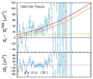
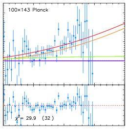
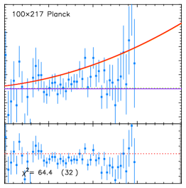
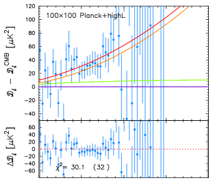
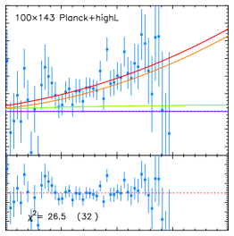
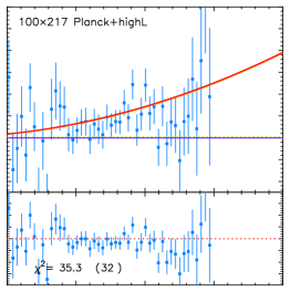
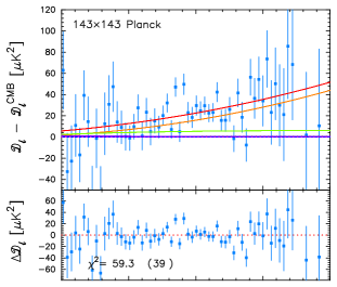
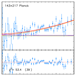
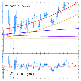
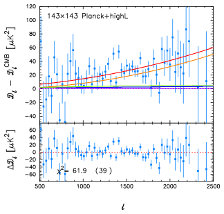
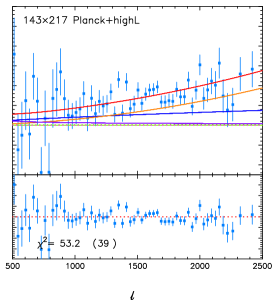
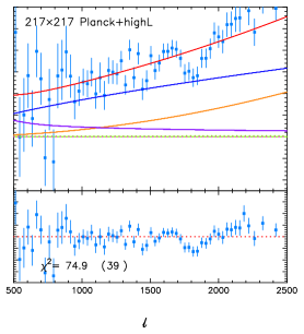
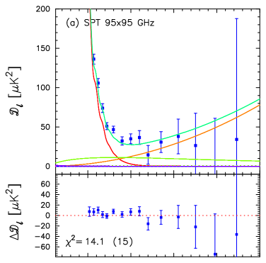
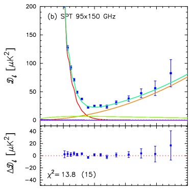
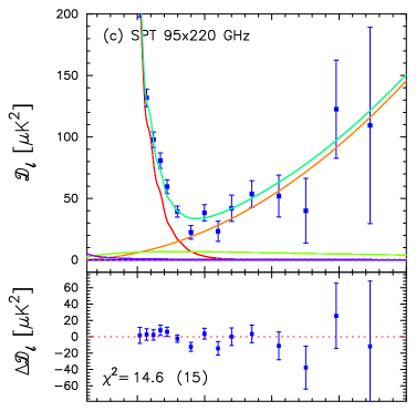
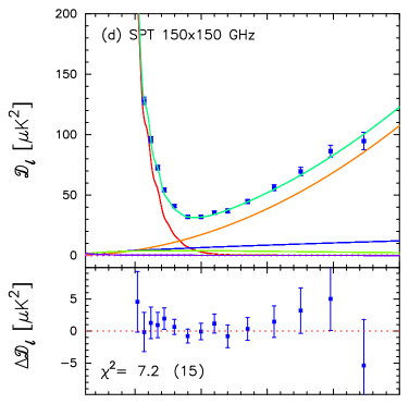
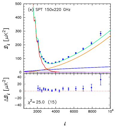
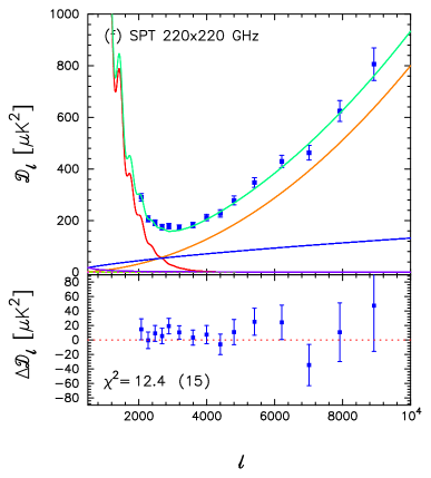
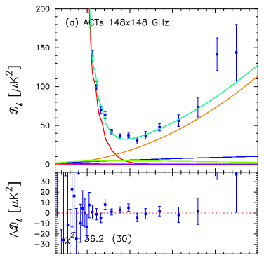
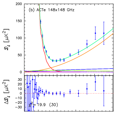
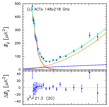
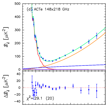
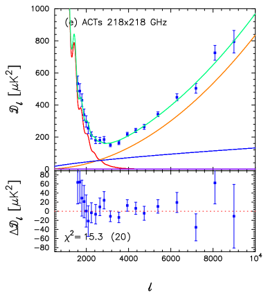
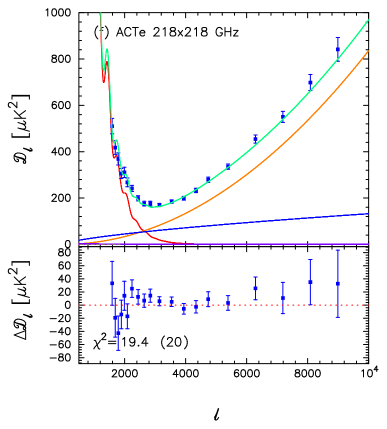
To quantify the consistency of the model fits shown in Fig. 7 for Planck we compute the $\chi^{2}$ statistic

$$\chi^{2}=\sum_{\ell\ell^{\prime}}(C_{\ell}^{\rm data}-C_{\ell}^{\rm CMB}-C_{\ell}^{\rm fg}){\cal M}^{-1}_{\ell\ell^{\prime}}(C_{\ell^{\prime}}^{\rm data}-C_{\ell^{\prime}}^{\rm CMB}-C_{\ell^{\prime}}^{\rm fg}),$$ (33)

for each of the spectra, where the sums extend over the multipole ranges $\ell_{\rm min}$ and $\ell_{\rm max}$ used in the likelihood, ${\cal M}_{\ell\ell^{\prime}}$ is the covariance matrix for the spectrum $C^{\rm data}_{\ell}$ (including corrections for beam eigenmodes and calibrations), $C_{\ell}^{\rm CMB}$ is the best-fit primordial CMB spectrum and $C_{\ell}^{\rm fg}$ is the best-fit foreground model appropriate to the data spectrum. We expect $\chi^{2}$ to be approximately Gaussian distributed with a mean of $N_{\ell}=\ell_{\rm max}-\ell_{\rm min}+1$ and dispersion $\sqrt{2N_{\ell}}$. Results are summarized in Table 6 for the Planck+WP+highL best-fit parameters of Table 5. (The $\chi^{2}$ values for the Planck+WP  fit are almost identical.) Each of the spectra gives an acceptable global fit to the model, quantifying the high degree of consistency of these spectra described in Planck Collaboration XV (2014). (Note that Planck Collaboration XV 2014 presents an alternative way of investigating consistency between these spectra via power spectrum differences.)

Figures 8 and 9 show the fits and residuals with respect to the best-fit Planck+WP+highL model of Table 5, for each of the SPT and ACT spectra. The SPT and ACT spectra are reported as band-powers, with associated window functions $[W^{\rm SPT}_{b}(\ell)/\ell]$ and $W^{\rm ACT}_{b}(\ell)$. The definitions of these window functions differ between the two experiments.

For SPT, the contribution of the CMB and foreground spectra in each band is

$${\cal D}_{b}=\sum_{\ell}[W_{b}^{\rm SPT}(\ell)/\ell]{\ell(\ell+1/2)\over 2\pi}\left(C^{\rm CMB}_{\ell}+C^{\rm fg}_{\ell}\right).$$ (34)

(Note that this differs from the equations given in R12 and S12.)

For ACT, the window functions operate on the power spectra:

$$C_{b}=\sum_{\ell}W_{b}^{\rm ACT}(\ell)\left(C^{\rm CMB}_{\ell}+C^{\rm fg}_{\ell}\right).$$ (35)

In Fig. 9. we plot ${\cal D}_{b}=\ell_{b}(\ell_{b}+1)C_{b}/(2\pi)$, where $\ell_{b}$ is the effective multipole for band $b$.

The upper panels of each of the sub-plots in Figs. 8 and 9 show the spectra of the best-fit CMB, and the total CMB+foreground, as well as the individual contributions of the foreground components using the same colour codings as in Fig. 7. The lower panel in each sub-plot shows the residuals with respect to the best-fit cosmology+foreground model. For each spectrum, we list the value of $\chi^{2}$, neglecting correlations between the (broad) ACT and SPT bands, together with the number of data points. The quality of the fits is generally very good. For SPT, the residuals are very similar to those inferred from Fig. 3 of R12. The SPT $150\times 220$ spectrum has the largest $\chi^{2}$ (approximately a $1.8\thinspace\sigma$ excess). This spectrum shows systematic positive residuals of a few ${\mu}{\rm K}^{2}$ over the entire multipole range. For ACT, the residuals and $\chi^{2}$ values are close to those plotted in Fig. 4 of Dunkley et al. (2013). All of the ACT spectra plotted in Fig. 9 are well fit by the model (except for some residuals at multipoles $\ell\la 2000$, which are also seen by Dunkley et al. 2013).

Figure 10: Planck $TT$ power spectrum. The points in the upper panel show the maximum-likelihood estimates of the primary CMB spectrum computed as described in the text for the best-fit foreground and nuisance parameters of the Planck+WP+highL fit listed in Table 5. The red line shows the best-fit base $\Lambda$CDM spectrum. The lower panel shows the residuals with respect to the theoretical model. The error bars are computed from the full covariance matrix, appropriately weighted across each band (see Eqs. 36a and 36b) and include beam uncertainties and uncertainties in the foreground model parameters.

Figure 11: Planck $TE$ (left) and $EE$ spectra (right) computed as described in the text. The red lines show the polarization spectra from the base $\Lambda$CDM Planck+WP+highL model, which is fitted to the TT data only.

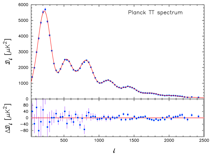
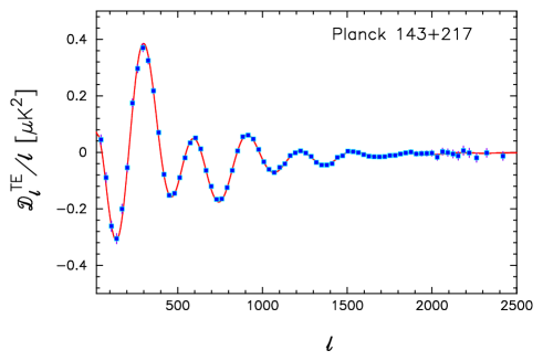
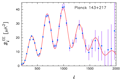
Having determined a solution for the best-fit foreground and other “nuisance” parameters, we can correct the four spectra used in the Planck likelihood and combine them to reconstruct a “best-fit” primary CMB spectrum and covariance matrix as described in  Planck Collaboration XV (2014). This best-fit Planck CMB spectrum is plotted in the upper panels of Figs. 1 and 10 for Planck+WP+highL foreground parameters. The spectrum in Fig. 10 has been band-averaged in bins of width $\Delta\ell\sim 31$ using a window function $W_{b}(l)$:

$$\hat{\cal D}_{b}=\sum_{\ell}W_{b}(\ell)\hat{\cal D}_{\ell},$$ (36a)

$$W_{b}(\ell)=\left\{\begin{array}[]{ll}(\hat{\cal M}^{\cal D}_{\ell\ell})^{-1}/\sum_{\ell=\ell^{b}_{\rm min}}^{\ell^{b}_{\rm max}}(\hat{\cal M}^{\cal D}_{\ell\ell})^{-1},&\ell^{b}_{\rm min}\leq\ell<\ell^{b}_{\rm max},\\ 0,&\mbox{otherwise}.\end{array}\right.$$ (36b)

Here, $\ell^{b}_{\rm min}$ and $\ell^{b}_{\rm max}$ denote the minimum and maximum multipole ranges of band $b$, and $\hat{\cal M}^{\cal D}_{\ell\ell^{\prime}}$ is the covariance matrix of the best-fit spectrum $\hat{\cal D}_{\ell}$, computed as described in Planck Collaboration XV (2014), and to which we have added corrections for beam and foreground errors (using the curvature matrix of the foreground model parameters from the MCMC chains). The solid lines in the upper panels of Figs. 1 and 10 show the spectrum for the best-fit $\Lambda$CDM cosmology. The residuals with respect to this cosmology are plotted in the lower panel. To assess the goodness-of-fit, we compute $\chi^{2}$:

$$\chi^{2}=\sum_{\ell\ell^{\prime}}(\hat{C}_{\ell}^{\rm data}-C_{\ell}^{\rm CMB})\hat{\cal M}^{-1}_{\ell\ell^{\prime}}(\hat{C}_{\ell^{\prime}}^{\rm data}-C_{\ell^{\prime}}^{\rm CMB}),$$ (37)

using the covariance matrix for the best-fit data spectrum (including foreground and beam errors). The results are given in the last line of Table 6 labelled “All.” The lower panel of Fig. 10 shows the residuals with respect to the best-fit cosmology (on an expanded scale compared to Fig. 1). There are some visually striking residuals in this plot, particularly in the regions $\ell\sim 800$ and $\ell\sim 1300$–$1500$ (where we see “oscillatory” behaviour). As discussed in detail in Planck Collaboration XV (2014), these residuals are reproducible to high accuracy across Planck detectors and across Planck frequencies; see also Fig. 7. There is therefore strong evidence that the residuals at these multipoles, which are in the largely signal dominated region of the spectrum, are real features of the primordial CMB sky. These features are compatible with statistical fluctuations of a Gaussian $\Lambda$CDM model, and are described accurately by the covariance matrix used in the Planck likelihood. As judged by the $\chi^{2}$ statistic listed in Table 6, the best fit reconstructed Planck spectrum is compatible with the base $\Lambda$CDM cosmology to within $1.6\thinspace\sigma$

To the extremely high accuracy afforded by the Planck data, the power spectrum at high multipoles is compatible with the predictions of the base six parameter $\Lambda$CDM cosmology. This is the main result of this paper. Fig. 1 does, however, suggest that the power spectrum of the best-fit base $\Lambda$CDM cosmology has a higher amplitude than the observed power spectrum at multipoles $\ell\la 30$. We will return to this point in Sect. 7.

Finally, Fig. 11 shows examples of Planck $TE$ and $EE$ spectra. These are computed by performing a straight average of the (scalar) beam-corrected $143\times 143$, $143\times 217$, and $217\times 217$ cross-spectra (ignoring auto-spectra). There are $32$ $TE$ and $ET$ cross-spectra contributing to the mean $TE$ spectrum plotted in Fig. 11, and six $EE$ spectra contributing to the mean $EE$ spectrum. Planck polarization data, including LFI and $353\thinspace$GHz data not shown here, will be analysed in detail, and incorporated into a Planck likelihood, following this data release. The purpose of presenting these figures here is twofold: first, to demonstrate the potential of Planck to deliver high quality polarization maps and spectra, as described in the Planck “blue-book” (Planck Collaboration 2005); and, second, to show the consistency of these polarization spectra with the temperature spectrum shown in Fig. 10. As discussed in Planck Collaboration VI (2014) and Planck Collaboration XV (2014), at present, the HFI polarization spectra at low multipoles ($\ell\la 200$) are affected by systematic errors that cause biases. For the HFI channels used in Fig. 11, there are two primary sources of systematic error arising from non-linear gain-like variations, and residual bandpass mismatches between detectors. However, these systematics rapidly become unimportant at higher multipoles.

The errors on the mean $TE$ and $EE$ spectra shown in Fig. 11 are computed from the analytic formulae given in Efstathiou (2006), using an effective beam-width adjusted to reproduce the observed scatter in the polarization spectra at high multipoles. The spectra are then band-averaged as in Eq. (37). The error bars shown in Fig. 11 are computed from the diagonal components of the band-averaged covariance matrices.

The solid lines in the upper panels of Fig. 11 show the theoretical $TE$ and $EE$ spectra expected in the best-fit Planck+WP+highL $\Lambda$CDM  model (i.e., the model used to compute the theory $TT$ spectrum plotted in Fig. 10). These theoretical spectra are determined entirely from the $TT$ analysis and make no use of the Planck polarization data. As with the $TT$ spectra, the $\Lambda$CDM model provides an extremely good match to the polarization spectra. Furthermore, polarized foreground emission is expected to be unimportant at high multipoles (e.g., Tucci & Toffolatti 2012) and so no foreground corrections have been made to the spectra in Fig. 11. The agreement between the polarization spectra and the theoretical spectra therefore provides strong evidence that the best-fit cosmological parameters listed in Table 5 are not strongly affected by the modelling of unresolved foregrounds in the $TT$ analysis.

5 Comparison of the Planck base $\Lambda$CDM model with other astrophysical data sets

Unlike CMB data, traditional astrophysical data sets – e.g., measurements of the Hubble parameter, type Ia supernovae (SNe Ia), and galaxy redshift surveys – involve complex physical systems that are not understood at a fundamental level. Astronomers are therefore reliant on internal consistency tests and empirical calibrations to limit the possible impact of systematic effects. Examples include calibrating the metallicity dependence of the Cepheid period luminosity relation, calibrating the colour-decline-rate-luminosity relation of Type Ia supernovae, or quantifying the relationship between the spatial distributions of galaxies and dark matter. In addition, there are more mundane potential sources of error, which can affect certain types of astrophysical observations (e.g., establishing consistent photometric calibration systems). We must be open to the possibility that unknown, or poorly quantified, systematic errors may be present in the astrophysical data, especially when used in combination with the high precision data from Planck.

We have seen in the previous section that the base $\Lambda$CDM model provides an acceptable fit to the Planck $TT$ power spectra (and the Planck $TE$ and $EE$ spectra) and also to the ACT and SPT temperature power spectra. The cosmological parameters of this model are determined to high precision. We therefore review whether these parameters provide acceptable fits to other astrophysical data. If they do not, then we need to assess whether the discrepancy is a pointer to new physics, or evidence of some type of poorly understood systematic effect. Unless stated otherwise, we use the Planck+WP+highL parameters listed in Table 5 as the default “Planck” parameters for the base $\Lambda$CDM  model.

5.1 CMB lensing measured by Planck

Figure 12: Planck measurements of the lensing power spectrum compared to the prediction for the best-fitting Planck+WP+highL $\rm{\Lambda CDM}$ model parameters. In the top panel, the data points are the measured bandpowers and $\pm 1\thinspace\sigma$ error ranges from the diagonal of the covariance matrix. The measured bandpowers are compared to the $C_{\ell}^{\phi\phi}$ in the best-fit model (black line). The grey region shows the $1\thinspace\sigma$ range in $C_{\ell}^{\phi\phi}$ due to $\rm{\Lambda CDM}$ parameter uncertainties. The lower panel shows the differences between the bandpower amplitudes $\hat{A}_{i}$ and the predictions for their expectation values in the best-fit model, $A_{i}^{\mbox{\scriptsize{theory}}}$.

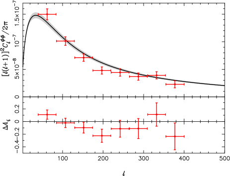
Weak gravitational lensing by large-scale structure subtly alters the statistics of the CMB anisotropies, encoding information about the late-time Universe which is otherwise degenerate in the primary anisotropies laid down at last-scattering (see Lewis & Challinor 2006 for a review). The lensing deflections are given by the gradient of the lensing potential $\phi(\hat{\@vec{n}})$, which corresponds to an integrated measure of the matter distribution along the line of sight with peak sensitivity to structures around redshift 2. The rms deflection is expected to be around $2.5\thinspace\mathrm{arcmin}$ and to be coherent over several degrees. We include the effect of lensing on the temperature power spectrum in all our parameter analysis, but for some results we also include the lensing information encoded in the non-Gaussian trispectrum (connected 4-point function) of the CMB. Lensing generates a non-zero trispectrum, which, at leading order, is proportional to the power spectrum $C_{\ell}^{\phi\phi}$ of the lensing potential (Hu 2001).

In Planck Collaboration XVII (2014), we present a detailed analysis of CMB lensing with Planck data, including estimation of $C_{\ell}^{\phi\phi}$ from the trispectrum computed from Planck’s maps. This paper also describes the construction of a lensing likelihood. Briefly, we first reconstruct an estimate of the lensing potential using near-optimal quadratic estimators, following Okamoto & Hu (2003), with various Galactic and point-source masks. The empirical power spectrum of this reconstruction, after subtraction of the Gaussian noise bias (i.e., the disconnected part of the 4-point function), is then used to estimate $C_{\ell}^{\phi\phi}$ in bandpowers. The associated bandpower errors are estimated from simulations. The lensing power spectrum is estimated from channel-coadded Planck maps at 100, 143 and 217 GHz in the multipole range $\ell=10$–$1000$, and also from a minimum-variance combination of the 143 and 217 GHz maps. An empirical correction for the shot-noise trispectrum of unresolved point sources is made to each spectrum, based on the measured amplitude of a generalized kurtosis of the appropriate maps. Additionally, the $N^{(1)}$ bias of Kesden et al. (2003), computed for a fiducial $\rm{\Lambda CDM}$ spectrum determined from a pre-publication analysis of the Planck data, is subtracted from each spectrum. This latter correction is proportional to $C_{\ell}^{\phi\phi}$ and accounts for sub-dominant couplings of the trispectrum, which mix lensing power over a range of scales into the power spectrum estimates. Excellent internal consistency of the various $C_{\ell}^{\phi\phi}$ estimates is found over the full multipole range.

The Planck lensing likelihood is based on reconstructions from the minimum-variance combination of the 143 and 217 GHz maps with 30% of the sky masked. Conservatively, only multipoles in the range $\ell=40$–$400$ are included, with a bandpower width $\Delta\ell=45$. The range $\ell=40$–$400$ captures 90% of the signal-to-noise on a measurement of the amplitude of a fiducial $C_{\ell}^{\phi\phi}$, while minimizing the impact of imperfections in modelling the effect of survey anisotropies on the large-scale $\phi$ reconstruction (the “mean-field” of Planck Collaboration XVII 2014), and the large Gaussian noise bias on small scales. Note, however, that by restricting the range of angular scales we do lose some ability to distinguish between scale-dependent modifications of $C_{\ell}^{\phi\phi}$, such as from massive neutrinos, and almost scale-independent modifications, such as from changes in the equation of state of unclustered dark energy or spatial curvature. Correlated uncertainties in the beam transfer functions, point-source corrections, and the cosmology dependence of the $N^{(1)}$ bias give very broad-band correlations between the bandpowers. These are modelled as a sum of rank-one corrections to the covariance matrix and induce bandpower correlations that are small, less than $4\%$, but very broad. Bandpower correlations induced by masking are estimated to be less than 5% for neighbouring bins and are neglected. The likelihood is modelled as a Gaussian in the bandpowers with a fiducial (i.e., parameter-independent) covariance. For verification of this approximation, see Schmittfull et al. (2013).

The connected four-point function is related to the fully-reduced trispectrum $\mathbb{T}^{\ell_{1}\ell_{2}}_{\ell_{3}\ell_{4}}(L)$ by

$$\langle T_{\ell_{1}m_{1}}T_{\ell_{2}m_{2}}T_{\ell_{3}m_{3}}T_{\ell_{4}m_{4}}\rangle_{\mathrm{c}} = \frac{1}{2}\sum_{LM}(-1)^{M}\left(\begin{array}[]{ccc}\ell_{1}&\ell_{2}&L\\ m_{1}&m_{2}&M\end{array}\right)$$ (43)

$$\mbox{}\times\left(\begin{array}[]{ccc}\ell_{3}&\ell_{4}&L\\ m_{3}&m_{4}&-M\end{array}\right)\mathbb{T}^{\ell_{1}\ell_{2}}_{\ell_{3}\ell_{4}}(L)+\mathrm{perms}\thinspace,$$

(Hu 2001). In the context of lensing reconstruction, the CMB trispectrum due to lensing takes the form

$$\mathbb{T}^{\ell_{1}\ell_{2}}_{\ell_{3}\ell_{4}}(L)\approx C_{L}^{\phi\phi}C_{\ell_{2}}^{TT}C_{\ell_{4}}^{TT}F_{\ell_{1}L\ell_{2}}F_{\ell_{3}L\ell_{4}}\thinspace,$$ (44)

where $C_{\ell}^{TT}$ is the lensed temperature power spectrum and $F_{\ell_{1}L\ell_{2}}$ is a geometric mode-coupling function (Hu 2001; Hanson et al. 2011). Our estimates of $C_{\ell}^{\phi\phi}$ derive from the measured trispectrum. They are normalized using the fiducial lensed power spectrum to account for the factors of $C_{\ell}^{TT}$ in Eq. (44). In the likelihood, we renormalize the parameter-dependent $C_{\ell}^{\phi\phi}$ to account for the mismatch between the parameter-dependent $C_{\ell}^{TT}$ and that in the fiducial model. Since the best-fit $\rm{\Lambda CDM}$ model we consider in this section has a lensed temperature power spectrum that is very close to that of the fiducial model, the renormalisation factor differs from unity by less than $0.25\%$.

The estimated lensing power spectrum $C_{\ell}^{\phi\phi}$ is not independent of the measured temperature power spectrum $C_{\ell}^{TT}$, but the dependence is very weak for Planck, and can be accurately ignored (Schmittfull et al. 2013; Planck Collaboration XVII 2014). As discussed in detail in Schmittfull et al. (2013), there are several effects to consider. First, the reconstruction noise in the estimated $\phi$ derives from chance correlations in the unlensed CMB. If, due to cosmic variance, the unlensed CMB fluctuates high at some scale, the noise in the reconstruction will generally increase over a broad range of scales. Over the scales relevant for Planck lensing reconstruction, the correlation between the measured $C_{\ell}^{\phi\phi}$ and $C_{\ell^{\prime}}^{TT}$ from this effect is less than $0.2\%$ and, moreover, is removed by a data-dependent Gaussian noise bias removal that we adopt following Hanson et al. (2011) and Namikawa et al. (2012). The second effect derives from cosmic variance of the lenses. If a lens on a given scale fluctuates high, the estimated $C_{\ell}^{\phi\phi}$ will fluctuate high at that scale. In tandem, there will be more smoothing of the acoustic peaks in the measured $C_{\ell^{\prime}}^{TT}$, giving broad-band correlations that are negative at acoustic peaks and positive at troughs. The maximum correlation is around $0.05\%$. If we consider estimating the amplitude of a fiducial lensing power spectrum independently from the smoothing effect of $C_{\ell}^{TT}$ and the measured $C_{\ell}^{\phi\phi}$ in the range $\ell=40$–$400$, the correlation between these estimates due to the cosmic variance of the lenses is only $4\%$. This amounts to a mis-estimation of the error on a lensing amplitude in a joint analysis of $C_{\ell}^{\phi\phi}$ and $C_{\ell}^{TT}$, treated as independent, of only $2\%$. For physical parameters, the mis-estimation of the errors is even smaller: Schmittfull et al. (2013) estimate around $0.5\%$ from a Fisher analysis. A third negligible effect is due to the $T$–$\phi$ correlation sourced by the late integrated Sachs-Wolfe effect (see Planck Collaboration XIX 2014). This produces only local correlations between the measured $C_{\ell}^{\phi\phi}$ and $C_{\ell}^{TT}$ which are less than $0.5\%$ by $\ell=40$ and fall rapidly on smaller scales. They produce a negligible correlation between lensing amplitude estimates for the multipole ranges considered here. The $T$–$\phi$ correlation is potentially a powerful probe of dark energy dynamics (e.g., Verde & Spergel 2002) and modified theories of gravity (e.g., Acquaviva et al. 2004). The power spectrum $C_{\ell}^{T\phi}$ can be measured from the Planck data using the CMB 3-point function (Planck Collaboration XXIV 2014) or, equivalently, by cross-correlating the $\phi$ reconstruction with the large-angle temperature anisotropies (Planck Collaboration XIX 2014) although the detection significance is only around $3\thinspace\sigma$. The power-spectrum based analysis in this paper discards the small amount of information in the $T$–$\phi$ correlation from Planck. In summary, we can safely treat the measured temperature and lensing power spectra as independent and simply multiply their respective likelihoods in a joint analysis.

We note that ACT (Das et al. 2011, 2013) and SPT (van Engelen et al. 2012) have both measured the lensing power spectrum with significances of $4.6\thinspace\sigma$ and $6.3\thinspace\sigma$, respectively, in the multipole ranges $\ell=75$–$2050$ and $\ell=100$–$1500$. The Planck measurements used here represent a $26\thinspace\sigma$ detection. We therefore do not expect the published lensing measurements from these other experiments to carry much statistical weight in a joint analysis with Planck, despite the complementary range of angular scales probed, and we choose not to include them in the analyses in this paper.

In the lensing likelihood, we characterize the estimates of $C_{\ell}^{\phi\phi}$ with a set of eight (dimensionless) amplitudes $\hat{A}_{i}$, where

$$\hat{A}_{i}=\sum_{\ell}\mathcal{B}^{\ell}_{i}\hat{C}_{\ell}^{\phi\phi}\thinspace.$$ (45)

Here, $\mathcal{B}^{\ell}_{i}$ is a binning operation with

$$\mathcal{B}^{\ell}_{i}=\frac{C_{\ell}^{\phi\phi,\thinspace\mathrm{fid}}V_{\ell}^{-1}}{\sum_{\ell^{\prime}=\ell_{\mathrm{min}}^{i}}^{\ell_{\mathrm{max}}^{i}}\left(C_{\ell^{\prime}}^{\phi\phi,\thinspace\mathrm{fid}}\right)^{2}V_{\ell^{\prime}}^{-1}}\thinspace,$$ (46)

for $\ell$ within the band defined by a minimum multipole $\ell_{\mathrm{min}}^{i}$ and a maximum $\ell_{\mathrm{max}}^{i}$. The inverse of the weighting function, $V_{\ell}$, is an approximation to the variance of the measured $\hat{C}_{\ell}^{\phi\phi}$ and $C_{\ell}^{\phi\phi,\thinspace\mathrm{fid}}$ is the lensing power spectrum of the fiducial model, which is used throughout the analysis. The $\hat{A}_{i}$ are therefore near-optimal estimates of the amplitude of the fiducial power spectrum within the appropriate multipole range, normalized to unity in the fiducial model. Given some parameter-dependent model $C_{\ell}^{\phi\phi}$, the expected values of the $\hat{A}_{i}$ are

$$\langle\hat{A}_{i}\rangle=A_{i}^{\mathrm{theory}}=\sum_{\ell}\mathcal{B}^{\ell}_{i}\left[1+\Delta^{\phi}(C_{\ell}^{TT})\right]^{2}C_{\ell}^{\phi\phi}\thinspace,$$ (47)

where the term involving $\Delta^{\phi}(C_{\ell}^{TT})$, which depends on the parameter-dependent $C_{\ell}^{TT}$, accounts for the renormalisation step described above. The lensing amplitudes $\hat{A}_{i}$ are compared to the $A_{i}^{\mbox{\scriptsize{theory}}}$ for the best-fitting $\rm{\Lambda CDM}$ model to the Planck+WP+highL data combination (i.e., not including the lensing likelihood) in Table 7. The differences between $\hat{A}_{i}$ and $A_{i}^{\mbox{\scriptsize{theory}}}$ are plotted in the bottom panel of Fig. 12 while in the top panel the bandpower estimates are compared to $C_{\ell}^{\phi\phi}$ in the best-fitting model. The Planck measurements of $C_{\ell}^{\phi\phi}$ are consistent with the prediction from the best-fit $\rm{\Lambda CDM}$ model to Planck+WP+highL. Using the full covariance matrix, we find $\chi^{2}=10.9$ with eight degrees of freedom, giving an acceptable probability to exceed of approximately $21\%$. It is worth recalling here that the parameters of the $\rm{\Lambda CDM}$ model are tightly constrained by the CMB 2-point function (as probed by our Planck+WP+highL data combination) which derives from physics at $z\approx 1100$ seen in angular projection. It is a significant further vindication of the $\rm{\Lambda CDM}$ model that its predictions for the evolution of structure and geometry at much lower redshifts (around $z=2$) fit so well with Planck’s CMB lensing measurements.

Table 7: Planck CMB lensing constraints. The $A_{i}^{\mbox{\scriptsize{theory}}}$ are renormalized power spectrum amplitudes in the best-fit $\rm{\Lambda CDM}$ model to Planck+WP+highL within the $i$th band (from $\ell_{\rm min}$ to $\ell_{\rm max}$). The errors $\sigma(A_{i})$ on the amplitudes are the square root of the diagonals of the $\hat{A}_{i}$ covariance matrix.

Band $$\ell_{\mathrm{min}}$$

1. 40 84 1.11 1.00 0.07

2. 85 129 0.97 0.99 0.07

3. 130 174 0.90 0.98 0.08

4. 175 219 0.77 0.98 0.10

5. 220 264 0.88 0.98 0.13

6. 265 309 0.88 0.98 0.16

7. 310 354 1.10 0.98 0.18

8. 355 400 0.75 0.98 0.21

The discussion above does not account for the small spread in the $C_{\ell}^{\phi\phi}$ predictions across the Planck+WP+highL $\rm{\Lambda CDM}$ posterior distribution. To address this, we introduce a parameter $A_{\rm L}^{\phi\phi}$ which, at any point in parameter space, scales the lensing trispectrum. Note that $A_{\rm L}^{\phi\phi}$ does not alter the lensed temperature power spectrum, so it can be used to assess directly how well the $\rm{\Lambda CDM}$ predictions from $C_{\ell}^{TT}$ agree with the lensing measurements; in $\rm{\Lambda CDM}$ we have $A_{\rm L}^{\phi\phi}=1$. The marginalized posterior distribution for $A_{\rm L}^{\phi\phi}$ in a joint analysis of Planck+WP+highL and the Planck lensing likelihood is given in Fig. 13. The agreement with $A_{\rm L}^{\phi\phi}=1$ is excellent, with

$$A_{\rm L}^{\phi\phi}=0.99\pm 0.05\quad(\mbox{68\%; {Planck}+lensing+WP+highL}).$$ (48)

The significance of the detection of lensing using $A_{\rm L}^{\phi\phi}$ in $\Lambda$CDM is a little less than the $26\thinspace\sigma$ detection of lensing power reported in Planck Collaboration XVII (2014), due to the small spread in $C_{\ell}^{\phi\phi}$ from $\Lambda$CDM parameter uncertainties.

Figure 13: Marginalized posterior distributions for $A_{\rm L}^{\phi\phi}$ (dashed) and $A_{\rm L}$ (solid). For $A_{\rm L}^{\phi\phi}$ we use the data combination Planck+lensing+WP+highL. For $A_{\rm L}$ we consider Planck+lensing+WP+highL (red), Planck+WP+highL (green), Planck+WP (blue) and Planck$-$lowL+highL+$\tau$prior (cyan; see text).

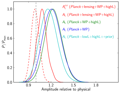
Lensing also affects the temperature power spectrum, primarily by smoothing the acoustic peaks and troughs on the scales relevant for Planck. The most significant detection of the lensing effect in the power spectrum to date is from SPT. Introducing a parameter $A_{\rm L}$ (Calabrese et al. 2008) which takes $C_{\ell}^{\phi\phi}\rightarrow A_{\rm L}C_{\ell}^{\phi\phi}$ when computing the lensed temperature power spectrum (we shall shortly extend the action of this parameter to include the computation of the lensing trispectrum), Story et al. (2012) report $A_{\rm L}=0.86^{+0.15}_{-0.13}$ (68%; SPT+WMAP-7). Results for $A_{\rm L}$ from Planck in combination with WMAP low-$\ell$ polarization and the high-$\ell$ power spectra from ACT and SPT are also shown in Fig. 13. Where we include the Planck lensing measurements, we define $A_{\rm L}$ to scale the explicit $C_{\ell}^{\phi\phi}$ in Eq. (44), as well as modulating the lensing effect in the temperature power spectrum. Figure 13 reveals a preference for $A_{\rm L}>1$ from the Planck temperature power spectrum (plus WMAP polarization). This is most significant when combining with the high-$\ell$ experiments for which we find

$$A_{\rm L}=1.23\pm 0.11\quad\mbox{(68\%; {Planck}+WP+highL)},$$ (49)

i.e., a $2\thinspace\sigma$ preference for $A_{\rm L}>1$. Including the lensing measurements, the posterior narrows but shifts to lower $A_{\rm L}$, becoming consistent with $A_{\rm L}=1$ at the $1\thinspace\sigma$ level as expected from the $A_{\rm L}^{\phi\phi}$ results.

Figure 14: Effect of allowing $A_{\rm L}$ to vary on the degeneracies between $\Omega_{\mathrm{b}}h^{2}$ and $n_{\rm s}$ (left) and $\Omega_{\mathrm{m}}h^{2}$ and $n_{\rm s}$ (right). In both panels the data combination is Planck+WP+highL. The contours enclose the $68\%$ and $95\%$ confidence regions in the base $\Lambda$CDM model with $A_{\rm L}=1$. The samples are from models with variable $A_{\rm L}$ and are colour-coded by the value of $A_{\rm L}$.

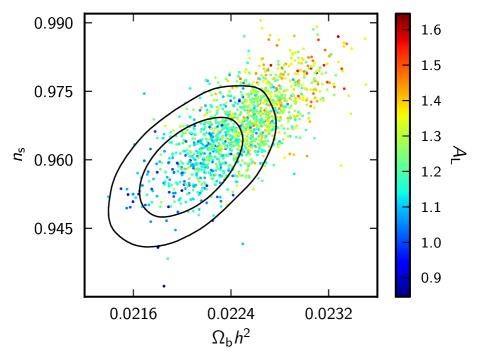
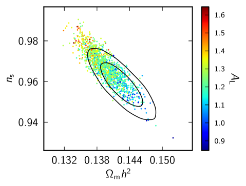
We do not yet have a full understanding of what is driving the preference for high $A_{\rm L}$ in the temperature power spectrum. As discussed in Appendix C, the general preference is stable to assumptions about foreground modelling and cuts of the Planck data in the likelihood. To gain some insight, we consider the range of multipoles that drive the preference for $A_{\rm L}>1$. For our favoured data combination of Planck+WP+highL, $\Delta\chi^{2}=-5.2$ going from the best-fit $A_{\rm L}=1$ model to the best-fit model with variable $A_{\rm L}$. The improvement in fit comes only from the low-$\ell$ temperature power spectrum ($\Delta\chi^{2}=-1.9$) and the ACT+SPT data ($\Delta\chi^{2}=-3.3$); for this data combination, there is no preference for high $A_{\rm L}$ from the Planck temperature data at intermediate and high multipoles ($\Delta\chi^{2}=+0.2$). The situation at low-$\ell$ is similar if we exclude the high-$\ell$ experiments, with $\Delta\chi^{2}=-1.6$ there, but there is then a preference for the high $A_{\rm L}$ best-fit from the Planck data on intermediate and small scales ($\Delta\chi^{2}=-3.4$). However, as discussed in Sect. 4, there is more freedom in the foreground model when we exclude the high-$\ell$ data, and this can offset smooth differences in the CMB power spectra such as the transfer of power from large to small scales by lensing that is enhanced for $A_{\rm L}>1$.

Since the low-$\ell$ temperature data seem to be partly responsible for pulling $A_{\rm L}$ high, we consider the effect of removing the low-$\ell$ likelihood from the analysis. In doing so, we also remove the WMAP large-angle polarization which we compensate by introducing a simple prior on the optical depth; we use a Gaussian with mean $0.09$ and standard deviation $0.013$, similar to the constraint from WMAP polarization (Hinshaw et al. 2012). We denote this data combination, including the high-$\ell$ experiments, by Planck$-$lowL+highL+$\tau$prior and show the posterior for $A_{\rm L}$ in Fig. 13. As anticipated, the peak of the posterior moves to lower $A_{\rm L}$ giving $A_{\rm L}=1.17^{+0.11}_{-0.13}$ (68% CL). The $\Delta\chi^{2}=+1.1$ between the best-fit model (now at $A_{\rm L}=1.18$) and the $A_{\rm L}=1$ model for the Planck data (i.e. no preference for the higher $A_{\rm L}$) while $\Delta\chi^{2}=-3.6$ for the high-$\ell$ experiments.

Since varying $A_{\rm L}$ alone does not alter the power spectrum on large scales, why should the low-$\ell$ data prefer higher $A_{\rm L}$? The reason is due to a chain of parameter degeneracies that are illustrated in Fig. 14, and the deficit of power in the measured $C_{\ell}$s on large scales compared to the best-fit $\Lambda$CDM model (see Fig. 1 and Sect. 7). In models with a power-law primordial spectrum, the temperature power spectrum on large scales can be reduced by increasing $n_{\rm s}$. The effect of an increase in $n_{\rm s}$ on the relative heights of the first few acoustic peaks can be compensated by increasing $\omega_{\mathrm{b}}$ and reducing $\omega_{\mathrm{m}}$, as shown by the contours in Fig. 14. However, on smaller scales, corresponding to modes that entered the sound horizon well before matter-radiation equality, the effects of baryons on the mid-point of the acoustic oscillations (which modulates the relative heights of even and odd peaks) is diminished since the gravitational potentials have pressure-damped away during the oscillations in the radiation-dominated phase (e.g., Hu & White 1996, 1997). Moreover, on such scales the radiation-driving at the onset of the oscillations that amplifies their amplitude happens early enough to be unaffected by small changes in the matter density. The net effect is that, in models with $A_{\rm L}=1$, the extent of the degeneracy involving $n_{\rm s}$, $\omega_{\mathrm{b}}$ and $\omega_{\mathrm{m}}$ is limited by the higher-order acoustic peaks, and there is little freedom to lower the large-scale temperature power spectrum by increasing $n_{\rm s}$ while preserving the good fit at intermediate and small scales. Allowing $A_{\rm L}$ to vary changes this picture, letting the degeneracy extend to higher $n_{\rm s}$, as shown by the samples in Fig. 14. The additional smoothing of the acoustic peaks due to an increase in $A_{\rm L}$ can mitigate the effect of increasing $n_{\rm s}$ around the fifth peak, where the signal-to-noise for Planck is still high. This allows one to decrease the spectrum at low $\ell$, while leaving it essentially unchanged on those smaller scales where Planck still has good sensitivity. Above $\ell\sim 2000$, the best-fit $A_{\rm L}$ model has a little more power than the base model (around $3\thinspace\mu\mathrm{K}^{2}$ at $\ell=2000$), while the Planck, ACT, and SPT data have excess power over the best-fit $A_{\rm L}=1$ $\Lambda$CDM+foreground model at the level of a few $\mu\mathrm{K}^{2}$ (see Sect. 4). It is plausible that this may drive the preference for high $A_{\rm L}$ in the $\chi^{2}$ of the high-$\ell$ experiments. We note that a similar $2\thinspace\sigma$ preference for $A_{\rm L}>1$ is also found combining ACT and WMAP data (Sievers et al. 2013) and, as we find here, this tension is reduced when the lensing power spectrum is included in the fit.

To summarize, there is no preference in the Planck lensing power spectrum for $A_{\rm L}>1$. The general preference for high $A_{\rm L}$ from the CMB power spectra in our favoured data combination (Planck+WP+highL) is mostly driven by two effects: the difficulty that $\Lambda$CDM models have in fitting the low-$\ell$ spectrum when calibrated from the smaller-scale spectrum; and, plausibly, from excess residuals at the $\mu\mathrm{K}^{2}$ level in the high-$\ell$ spectra relative to the best-fit $A_{\rm L}=1$ $\Lambda$CDM+foregrounds model on scales where extragalactic foreground modelling is critical.

5.2 Baryon acoustic oscillations

Baryon acoustic oscillations (BAO) in the matter power spectrum were first detected in analyses of the 2dF Galaxy Redshift Survey (Cole et al. 2005) and the SDSS redshift survey (Eisenstein et al. 2005). Since then, accurate BAO measurements have been made using a number of different galaxy redshift surveys, providing constraints on the distance luminosity relation spanning the redshift range $0.1\la z\la 0.7$. Here we use the results from four redshift surveys: the SDSS DR7 BAO measurements at effective redshifts $z_{\rm eff}=0.2$ and $z_{\rm eff}=0.35$, analysed by Percival et al. (2010); the $z=0.35$ SDSS DR7 measurement at $z_{\rm eff}=0.35$ reanalyzed by Padmanabhan et al. (2012); the WiggleZ measurements at $z_{\rm eff}=0.44$, $0.60$ and $0.73$ analysed by Blake et al. (2011); the BOSS DR9 measurement at $z_{\rm eff}=0.57$ analyzed by Anderson et al. (2012); and the 6dF Galaxy Survey measurement at $z=0.1$ discussed by Beutler et al. (2011).

BAO surveys measure the distance ratio

$$d_{z}={r_{\rm s}(z_{\rm drag})\over D_{\rm V}(z)},$$ (50)

where $r_{\rm s}(z_{\rm drag})$ is the comoving sound horizon at the baryon drag epoch (when baryons became dynamically decoupled from the photons) and $D_{\rm V}(z)$ is a combination of the angular-diameter distance, $D_{\rm A}(z)$, and the Hubble parameter, $H(z)$, appropriate for the analysis of spherically-averaged two-point statistics:

$$D_{\rm V}(z)=\left[(1+z)^{2}D^{2}_{\rm A}(z){cz\over H(z)}\right]^{1/3}.$$ (51)

In the $\rm{\Lambda CDM}$ cosmology (allowing for spatial curvature), the angular diameter distance to redshift $z$ is

$$D_{\rm A}(z) = {c\over H_{0}}\hat{D}_{\rm A}.$$ (52)

$$= {c\over H_{0}}{1\over|\Omega_{K}|^{1/2}(1+z)}{\rm sin}_{K}\left[|\Omega_{K}|^{1/2}x(z,\Omega_{\rm m},\Omega_{\Lambda})\right],$$

where

$$x(z,\Omega_{\rm m},\Omega_{\Lambda})=\int_{0}^{z}{dz^{\prime}\over[\Omega_{\rm m}(1+z^{\prime})^{3}+\Omega_{K}(1+z^{\prime})^{2}+\Omega_{\Lambda}]^{1/2}},$$ (53)

and ${\rm sin}_{K}={\rm sinh}$ for $\Omega_{K}>0$ and ${\rm sin}_{K}=\sin$ for $\Omega_{K}<0$. (The small effects of the $0.06\thinspace{\rm eV}$ massive neutrino in our base cosmology are ignored in Eq. 53.) Note that the luminosity distance, $D_{\rm L}$, relevant for the analysis of Type Ia supernovae (see Sect.  5.4) is related to the angular diameter distance via $D_{\rm L}=(c/H_{0})\hat{D}_{\rm L}=D_{\rm A}(1+z)^{2}$.

Figure 15: Acoustic-scale distance ratio $r_{\rm s}/D_{\rm V}(z)$ divided by the distance ratio of the Planck base $\rm{\Lambda CDM}$ model. The points are colour-coded as follows: green star (6dF); purple squares (SDSS DR7 as analyzed by Percival et al. 2010); black star (SDSS DR7 as analyzed by Padmanabhan et al. 2012); blue cross (BOSS DR9); and blue circles (WiggleZ). The grey band shows the approximate $\pm 1\thinspace\sigma$ range allowed by Planck (computed from the CosmoMC chains).

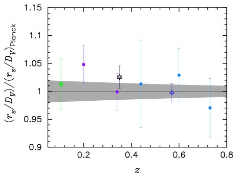
Different groups fit and characterize BAO features in different ways. For example, the WiggleZ team encode some shape information on the power spectrum to measure the acoustic parameter $A(z)$, introduced by Eisenstein et al. (2005),

$$A(z)={D_{\rm V}(z)\sqrt{\Omega_{\mathrm{m}}H_{0}^{2}}\over cz},$$ (54)

which is almost independent of $\omega_{\rm m}$. To simplify the presentation, Fig. 15 shows estimates of $r_{\rm s}/D_{\rm V}(z)$ and $1\thinspace\sigma$ errors, as quoted by each of the experimental groups, divided by the expected relation for the Planck  base $\rm{\Lambda CDM}$  parameters. Note that the experimental groups use the approximate formulae of Eisenstein & Hu (1998) to compute $z_{\rm drag}$ and $r_{\rm s}(z_{\rm drag})$, though they fit power spectra computed with Boltzmann codes, such as camb, generated for a set of fiducial-model parameters. The measurements have now become so precise that the small difference between the Eisenstein & Hu (1998) approximations and the accurate values of $z_{\rm drag}$ and $r_{\rm drag}=r_{\rm s}(z_{\rm drag})$ returned by camb need to be taken into account. In CosmoMC we multiply the accurate numerical value of $r_{\rm s}(z_{\rm drag})$ by a constant factor of $1.0275$ to match the Eisenstein-Hu approximation in the fiducial model. This correction is sufficiently accurate over the range of $\omega_{\rm m}$ and $\omega_{\rm b}$ allowed by the CMB in the base $\Lambda$CDM cosmology (see e.g. Mehta et al. 2012) and also for the extended $\Lambda$CDM models discussed in Sect. 6.

The Padmanabhan et al. (2012) result plotted in Fig. 15 is a reanalysis of the $z_{\rm eff}=0.35$ SDSS DR7 sample discussed by Percival et al. (2010). Padmanabhan et al. (2012) achieve a higher precision than Percival et al. (2010) by employing a reconstruction technique (Eisenstein et al. 2007) to correct (partially) the baryon oscillations for the smearing caused by galaxy peculiar velocities. The Padmanabhan et al. (2012) results are therefore strongly correlated with those of Percival et al. (2010). We refer to the Padmanabhan et al. (2012) “reconstruction-corrected” results as SDSS(R). A similar reconstruction technique was applied to the BOSS survey by Anderson et al. (2012) to achieve $1.6\%$ precision in $D_{\rm V}(z=0.57)/r_{\rm s}$, the most precise determination of the acoustic oscillation scale to date.

All of the BAO measurements are compatible with the base $\rm{\Lambda CDM}$ parameters from Planck. The grey band in Fig. 15 shows the $\pm 1\thinspace\sigma$ range in the acoustic-scale distance ratio computed from the Planck+WP+highL  CosmoMC chains for the base $\Lambda$CDM model. To get a qualitative feel for how the BAO measurements constrain parameters in the base $\Lambda$CDM model, we form $\chi^{2}$,

$$\chi_{\rm BAO}^{2}=({\mbox{\boldmath{$x$}}}-{\mbox{\boldmath{$x$}}}^{\Lambda{\rm CDM}})^{T}\@tens{C}_{\rm BAO}^{-1}({\mbox{\boldmath{$x$}}}-{\mbox{\boldmath{$x$}}}^{\Lambda{\rm CDM}}),$$ (55)

where $x$ is the data vector, ${\mbox{\boldmath{$x$}}}^{\Lambda{\rm CDM}}$ denotes the theoretical prediction for the $\rm{\Lambda CDM}$ model and $\@tens{C}_{\rm BAO}^{-1}$ is the inverse covariance matrix for the data vector $x$. The data vector is as follows: $D_{\rm V}(0.106)=(457\pm 27)\thinspace{\rm Mpc}$ (6dF); $r_{\rm s}/D_{\rm V}(0.20)=0.1905\pm 0.0061$, $r_{\rm s}/D_{\rm V}(0.35)=0.1097\pm 0.0036$ (SDSS); $A(0.44)=0.474\pm 0.034$, $A(0.60)=0.442\pm 0.020$, $A(0.73)=0.424\pm 0.021$ (WiggleZ); $D_{\rm V}(0.35)/r_{\rm s}=8.88\pm 0.17$ (SDSS(R)); and $D_{\rm V}(0.57)/r_{\rm s}=13.67\pm 0.22$, (BOSS). The off-diagonal components of $\@tens{C}_{\rm BAO}^{-1}$ for the SDSS and WiggleZ results are given in Percival et al. (2010) and Blake et al. (2011). We ignore any covariances between surveys. Since the SDSS and SDSS(R) results are based on the same survey, we include either one set of results or the other in the analysis described below, but not both together.

The Eisenstein-Hu values of $r_{\rm s}$ for the Planck and WMAP-9 base $\rm{\Lambda CDM}$ parameters differ by only $0.9\%$, significantly smaller than the errors in the BAO measurements. We can obtain an approximate idea of the complementary information provided by BAO measurements by minimizing Eq. (55) with respect to either $\Omega_{\rm m}$ or $H_{0}$, fixing $\omega_{\rm m}$ and $\omega_{\rm b}$ to the CMB best-fit parameters. (We use the Planck+WP+highL parameters from Table 5.) The results are listed in Table 8.

Table 8: Approximate constraints with 68% errors on $\Omega_{\rm m}$ and $H_{0}$ (in units of ${\rm km}\thinspace{\rm s}^{-1}\thinspace{\rm Mpc}^{-1}$) from BAO, with $\omega_{\rm m}$ and $\omega_{\rm b}$ fixed to the best-fit Planck+WP+highL values for the base $\Lambda$CDM cosmology.

Sample       $$\Omega_{\rm m} H_{0} 0.305^{+0.032}_{-0.026} 68.3^{+3.2}_{-3.2} 0.295^{+0.019}_{-0.017} 69.5^{+2.2}_{-2.1} 0.293^{+0.015}_{-0.013} 69.6^{+1.7}_{-1.5} 0.309^{+0.041}_{-0.035} 67.8^{+4.1}_{-2.8} 0.315^{+0.015}_{-0.015} 67.2^{+1.6}_{-1.5} 0.307^{+0.010}_{-0.011} 68.1^{+1.1}_{-1.1} 0.305^{+0.009}_{-0.010} 68.4^{+1.0}_{-1.0} 0.305^{+0.009}_{-0.008} 68.4^{+1.0}_{-1.0}$$        6dF.               SDSS.               SDSS(R).               WiggleZ.               BOSS.               6dF+SDSS+BOSS+WiggleZ.               6dF+SDSS(R)+BOSS.               6dF+SDSS(R)+BOSS+WiggleZ.              

As can be seen, the results are very stable from survey to survey and are in excellent agreement with the base $\rm{\Lambda CDM}$ parameters listed in Tables 2 and 5. The values of $\chi^{2}_{\rm BAO}$ are also reasonable. For example, for the six data points of the 6dF+SDSS(R)+BOSS+WiggleZ combination, we find $\chi^{2}_{\rm BAO}=4.3$, evaluated for the Planck+WP+highL best-fit $\rm{\Lambda CDM}$ parameters.

The high value of $\Omega_{\mathrm{m}}$ is consistent with the parameter analysis described by Blake et al. (2011) and with the “tension” discussed by Anderson et al. (2012) between BAO distance measurements and direct determinations of $H_{0}$ (Riess et al. 2011; Freedman et al. 2012). Furthermore, if the errors on the BAO measurements are accurate, the constraints on $\Omega_{\mathrm{m}}$ and $H_{0}$ (for fixed $\omega_{\rm m}$ and $\omega_{\rm b}$) are of comparable accuracy to those from Planck.

The results of this section show that BAO measurements are an extremely valuable complementary data set to Planck. The measurements are basically geometrical and free from complex systematic effects that plague many other types of astrophysical measurements. The results are consistent from survey to survey and are of comparable precision to Planck. In addition, BAO measurements can be used to break parameter degeneracies that limit analyses based purely on CMB data. For example, from the excellent agreement with the base $\rm{\Lambda CDM}$ model evident in Fig. 15, we can infer that the combination of Planck and BAO measurements will lead to tight constraints favouring $\Omega_{K}=0$ (Sect. 6.2) and a dark energy equation-of-state parameter, $w=-1$ (Sect. 6.5). Since the BAO measurements are primarily geometrical, they are used in preference to more complex astrophysical datasets to break CMB parameter degeneracies in this paper.

Finally, we note that we choose to use the 6dF+SDSS(R)+BOSS data combination in the likelihood analysis of Sect. 6. This choice includes the two most accurate BAO measurements and, since the effective redshifts of these samples are widely separated, it should be a very good approximation to neglect correlations between the surveys.

5.3 The Hubble constant

Figure 16: Comparison of $H_{0}$ measurements, with estimates of $\pm 1\thinspace\sigma$ errors, from a number of techniques (see text for details). These are compared with the spatially-flat $\rm{\Lambda CDM}$ model constraints from Planck and WMAP-9.

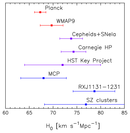
A striking result from the fits of the base $\rm{\Lambda CDM}$ model to Planck power spectra is the low value of the Hubble constant, which is tightly constrained by CMB data alone in this model. From the Planck+WP+highL  analysis we find

$$H_{0}=(67.3\pm 1.2)\thinspace{\rm km}\thinspace{\rm s}^{-1}\thinspace{\rm Mpc}^{-1}\quad\mbox{(68\%; {Planck}+WP+highL)}.$$ (56)

A low value of $H_{0}$ has been found in other CMB experiments, most notably from the recent WMAP-9 analysis. Fitting the base $\rm{\Lambda CDM}$ model, Hinshaw et al. (2012) find

$$H_{0}=(70.0\pm 2.2)\thinspace{\rm km}\thinspace{\rm s}^{-1}\thinspace{\rm Mpc}^{-1}\quad\mbox{(68\%; \ {WMAP}-9}),$$ (57)

consistent with Eq. (56) to within $1\thinspace\sigma$. We emphasize here that the CMB estimates are highly model dependent. It is important therefore to compare with astrophysical measurements of $H_{0}$, since any discrepancies could be a pointer to new physics.

Figure 17: MCMC samples and contours in the $r_{\ast}$–$\Omega_{\mathrm{m}}h^{2}$ plane (left) and the $D_{\rm A}(z_{\ast})$–$\Omega_{\mathrm{m}}h^{2}$ plane (right) for $\Lambda$CDM models analysed with Planck+WP+highL. The lines in these plots show the expected degeneracy directions in the base $\Lambda$CDM cosmology. Samples are colour-coded by the values of $\Omega_{\mathrm{b}}h^{2}$ (left) and $H_{0}$ (right).

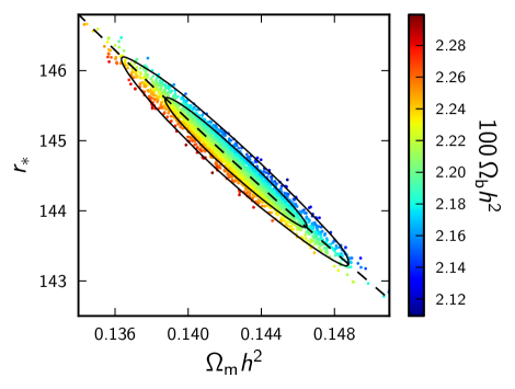
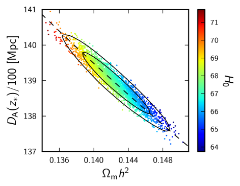
There have been remarkable improvements in the precision of the cosmic distance scale in the last decade or so. The final results of the Hubble Space Telescope (HST) Key Project (Freedman et al. 2001), which used Cepheid calibrations of secondary distance indicators, resulted in a Hubble constant of $H_{0}=(72\pm 8)\thinspace{\rm km}\thinspace{\rm s}^{-1}\thinspace{\rm Mpc}^{-1}$ (where the error includes estimates of both $1\thinspace\sigma$ random and systematic errors). This estimate has been used widely in combination with CMB observations and other cosmological data sets to constrain cosmological parameters (e.g., Spergel et al. 2003, 2007). It has also been recognized that an accurate measurement of $H_{0}$ with around 1% precision, when combined with CMB and other cosmological data, has the potential to reveal exotic new physics, for example, a time-varying dark energy equation of state, additional relativistic particles, or neutrino masses (see e.g., Suyu et al. 2012, and references therein). Establishing a more accurate cosmic distance scale is, of course, an important problem in its own right. The possibility of uncovering new fundamental physics provides an additional incentive.

Two recent analyses have greatly improved the precision of the cosmic distance scale. Riess et al. (2011) use HST observations of Cepheid variables in the host galaxies of eight SNe Ia to calibrate the supernova magnitude-redshift relation. Their “best estimate” of the Hubble constant, from fitting the calibrated SNe magnitude-redshift relation, is

$$H_{0}=(73.8\pm 2.4)\thinspace{\rm km}\thinspace{\rm s}^{-1}\thinspace{\rm Mpc}^{-1}\quad\mbox{(Cepheids+SNe Ia)},$$ (58)

where the error is $1\thinspace\sigma$ and includes known sources of systematic errors. At face value, this measurement is discrepant with the Planck  estimate in Eq. (56) at about the $2.5\thinspace\sigma$ level.

Freedman et al. (2012), as part of the Carnegie Hubble Program, use Spitzer Space Telescope mid-infrared observations to recalibrate secondary distance methods used in the HST Key Project. These authors find

$$H_{0} = [74.3\pm 1.5\thinspace\thinspace\mbox{(statistical)}\pm 2.1\thinspace\thinspace\mbox{(systematic)}]\thinspace{\rm km}\thinspace{\rm s}^{-1}\thinspace{\rm Mpc}^{-1}$$ (59)

$$\hskip 86.72267pt\mbox{(Carnegie HP)}.$$

We have added the two sources of error in quadrature in the error range shown in Fig. 16. This estimate agrees well with Eq. (58) and is also discordant with the Planck value (Eq. 16) at about the $2.5\thinspace\sigma$ level. The error analysis in Eq. (59) does not include a number of known sources of systematic error and is very likely an underestimate. For this reason, and because of the relatively good agreement between Eqs. (58) and (59), we do not use the estimate in Eq. (59) in the likelihood analyses described in Sect. 6.

The dominant source of error in the estimate in Eq. (58) comes from the first rung in the distance ladder. Using the megamaser-based distance to NGC4258, Riess et al. (2011) find $(74.8\pm 3.1)\thinspace{\rm km}\thinspace{\rm s}^{-1}\thinspace{\rm Mpc}^{-1}$. Using parallax measurements for 10 Milky Way Cepheids, they find $(75.7\pm 2.6)\thinspace{\rm km}\thinspace{\rm s}^{-1}\thinspace{\rm Mpc}^{-1}$, and using Cepheid observations and a revised distance to the Large Magellanic Cloud, they find $(71.3\pm 3.8)\thinspace{\rm km}\thinspace{\rm s}^{-1}\thinspace{\rm Mpc}^{-1}$. These estimates are consistent with each other, and the combined estimate in Eq. (58) uses all three calibrations. The fact that the error budget of measurement (58) is dominated by the “first-rung” calibrators is a point of concern. A mild underestimate of the distance errors to these calibrators could eliminate the tension with Planck.

Figure 16 includes three estimates of $H_{0}$ based on “geometrical” methods. The estimate labelled “MCP” shows the result $H_{0}=(68.0\pm 4.8)\thinspace{\rm km}\thinspace{\rm s}^{-1}\thinspace{\rm Mpc}^{-1}$ from the Megamaser Cosmology Project (Braatz et al. 2013) based on observations of megamasers in UGC 3789, NGC 6264 and Mrk 1419 (see also Reid et al. 2012, for a detailed analysis of UGC 3789). The point labelled “RXJ1131-1231” shows the estimate $H_{0}=78.7^{+4.3}_{-4.5}\thinspace{\rm km}\thinspace{\rm s}^{-1}\thinspace{\rm Mpc}^{-1}$ derived from gravitational lensing time delay measurements of the system RXJ1131-1231, observed as part of the “COSmological MOnitoring of GRAvitational Lenses” (COSMOGRAIL) project (Suyu et al. 2013, see also Courbin et al. 2011; Tewes et al. 2013). Finally, the point labelled SZ clusters shows the value $H_{0}=76.9^{+10.7}_{-8.7}\thinspace{\rm km}\thinspace{\rm s}^{-1}\thinspace{\rm Mpc}^{-1}$ (Bonamente et al. 2006), derived by combining tSZ and X-ray measurements of rich clusters of galaxies (see Carlstrom et al. 2002, and references therein). These geometrical methods bypass the need for local distance calibrators, but each has its own sources of systematic error that need to be controlled. The geometrical methods are consistent with the Cepheid-based methods, but at present, the errors on these methods are quite large. The COSMOGRAIL measurement (which involved a “blind” analysis to prevent experimenter bias) is discrepant at about $2.5\thinspace\sigma$ with the Planck value in Eq. (56). We note here a number of other direct measurements of $H_{0}$ (Jones et al. 2005; Sandage et al. 2006; Oguri 2007; Tammann & Reindl 2013) that give lower values than the measurements summarized in Fig. 16.

The tension between the CMB-based estimates and the astrophysical measurements of $H_{0}$ is intriguing and merits further discussion. In the base $\rm{\Lambda CDM}$ model, the sound horizon depends primarily on $\Omega_{\mathrm{m}}h^{2}$ (with a weaker dependence on $\Omega_{\mathrm{b}}h^{2}$). This is illustrated by the left-hand panel of Fig. 17, which shows samples from the Planck+WP+highL MCMC chains in the $r_{\ast}$–$\Omega_{\rm m}h^{2}$ plane colour coded according to $\Omega_{\rm b}h^{2}$. The acoustic scale parameter $\theta_{*}$ is tightly constrained by the CMB power spectrum, and so a change in $r_{\ast}$ must be matched by a corresponding shift in the angular diameter distance to the last scattering surface $D_{\rm A}(z_{\ast})$. In the base $\rm{\Lambda CDM}$ model, $D_{\rm A}$ depends on $H_{0}$ and $\Omega_{\rm m}h^{2}$, as shown in the right-hand panel of Fig. 17. The $2.7\thinspace{\rm km}\thinspace{\rm s}^{-1}\thinspace{\rm Mpc}^{-1}$ shift in $H_{0}$ between Planck and WMAP-9 is primarily a consequence of the slightly higher matter density determined by Planck ($\Omega_{\rm m}h^{2}=0.143\pm 0.003$) compared to WMAP-9 ($\Omega_{\rm m}h^{2}=0.136\pm 0.004$). A shift of around $7\thinspace{\rm km}\thinspace{\rm s}^{-1}\thinspace{\rm Mpc}^{-1}$, necessary to match the astrophysical measurements of $H_{0}$ would require an even larger change in $\Omega_{\rm m}h^{2}$, which is disfavoured by the Planck data. The tension between Planck and the direct measurements of $H_{0}$ cannot be easily resolved by varying the parameters of the base $\rm{\Lambda CDM}$ model. Section 6 will explore whether there are any extensions to the base $\rm{\Lambda CDM}$ model that can relieve this tension. In that section, results labelled “$H_{0}$” include a Gaussian prior on $H_{0}$ based on the Riess et al. (2011) measurement given in Eq. (58).

5.4 Type Ia supernovae

Figure 18: Magnitude residuals relative to the base $\Lambda$CDM model that best fits the SNLS combined sample (left) and the Union2.1 sample (right). The error bars show the $1\thinspace\sigma$ (diagonal) errors on $m_{B}$. The filled grey regions show the residuals between the expected magnitudes and the best-fit to the SNe sample as $\Omega_{\mathrm{m}}$ varies across the $\pm 2\thinspace\sigma$ range allowed by Planck+WP+highL in the base $\Lambda$CDM cosmology. The colour coding of the SNLS samples are as follows: low redshift (blue points); SDSS (green points); SNLS three-year sample (orange points); and HST high redshift (red points).

Table 9: Best-fit parameters for the SNLS compilations.

Data set       $$N_{\rm SNe}$$                                          

SNLS combined.       472                     1.425       3.256       0.227       407.8

SNLS SiFTO.       468                     1.352       3.375       0.223       414.9

SNLS SALT2.       473                     1.698       3.289       0.247       376.7

SNLS combined (CMB ).       472                     1.417       3.244       0.317       412.5

SNLS SiFTO (CMB ).       468                     1.339       3.351       0.317       420.1

SNLS SALT2 (CMB ).       473                     1.691       3.302       0.317       378.9

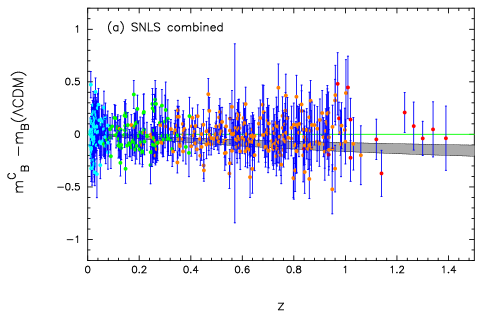
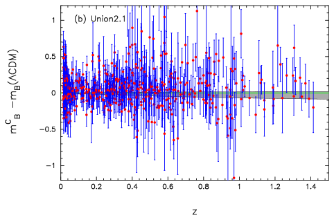
In this subsection, we analyse two SNe Ia samples: the sample of $473$ SNe as reprocessed by Conley et al. (2011), which we will refer to as the “SNLS” compilation; and the updated Union2.1 compilation of 580 SNe described by Suzuki et al. (2012).

5.4.1 The SNLS compilation

The SNLS “combined” compilation consists of $123$ SNe Ia at low redshifts, $242$ SNe Ia from the three-year Supernova Legacy Survey (SNLS; see Regnault et al. 2009; Guy et al. 2010; Conley et al. 2011), 93 intermediate redshift SNe Ia from the Sloan Digital Sky Survey (SDSS; Holtzman et al. 2008; Kessler et al. 2009) and 14 objects at high redshift observed with the Hubble Space Telescope (HST; Riess et al. 2007).

The “combined” sample of Conley et al. (2011) combines the results of two light-curve fitting codes, SiFTO (Conley et al. 2008) and SALT2 (Guy et al. 2007), to produce a peak apparent $B$-band magnitude, $m_{B}$, stretch parameter $s$ and colour ${\cal C}$ for each supernova. To explore the impact of light-curve fitting, we also analyse separately the SiFTO and SALT2 parameters. The SiFTO and SALT2 samples differ by a few SNe from the combined sample because of colour and stretch constraints imposed on the samples. We also use ancillary data, such as estimates of the stellar masses of the host galaxies and associated covariance matrices, as reported by Conley et al. (2011).

In this section, we focus exclusively on the base $\Lambda$CDM model (i.e., $w=-1$ and $\Omega_{K}=0$). For a flat Universe, the expected apparent magnitudes are then given by

$$m^{\Lambda{\rm CDM}}_{B}=5{\rm log}_{10}\hat{D}_{\rm L}(z_{\rm hel},z_{\rm CMB},\Omega_{\mathrm{m}})-\alpha(s-1)+\beta{\cal C}+{\cal M}_{B},$$ (60)

where $\hat{D}_{\rm L}$ is the dimensionless luminosity distance and ${\cal M}_{B}$ absorbs the Hubble constant. As in Sullivan et al. (2011), we express values of the parameter(s) ${\cal M}_{B}$ in terms of an effective absolute magnitude

$$M_{B}={\cal M}_{B}-5{\rm log}_{10}\left({c\over H_{0}}\right)-25,$$ (61)

for a value of $H_{0}=70\thinspace{\rm km}\thinspace{\rm s}^{-1}\thinspace{\rm Mpc}^{-1}$.

The likelihood for this sample is then constructed as in Conley et al. (2011) and Sullivan et al. (2011):

$$\chi_{\rm SNe}^{2}=({\mbox{\boldmath{$M$}}}_{B}-{\mbox{\boldmath{$M$}}}^{\Lambda{\rm CDM}}_{B})^{T}\@tens{C}_{\rm SNe}^{-1}({\mbox{\boldmath{$M$}}}_{B}-{\mbox{\boldmath{$M$}}}^{\Lambda{\rm CDM}}_{B}),$$ (62)

where ${\mbox{\boldmath{$M$}}}_{B}$ is the vector of effective absolute magnitudes and $\@tens{C}_{\rm SNe}$ is the sum of the non-sparse covariance matrices of Conley et al. (2011) quantifying statistical and systematic errors. As in Sullivan et al. (2011), we divide the sample according to the estimated stellar mass of the host galaxy and solve for two parameters, $M^{1}_{B}$ for $M_{\rm host}<10^{10}{\rm M}_{\odot}$ and $M^{2}_{B}$ for $M_{\rm host}\geq 10^{10}{\rm M}_{\odot}$. We adopt the estimates of the “intrinsic” scatter in $m_{B}$ for each SNe sample given in Table 4 of Conley et al. (2011).

Fits to the SNLS combined sample are shown in the left-hand panel of Fig. 18. The best-fit parameters for the combined, SiFTO and SALT2 samples are given in Table 9. In the base $\Lambda$CDM model, the SNe data provide a constraint on $\Omega_{\mathrm{m}}$, independent of the CMB. As can be seen from Table 9 (and also in the analyses of Conley et al. 2011 and Sullivan et al. 2011), the SNLS combined compilation favours a lower value of $\Omega_{\mathrm{m}}$ than we find from the CMB. The key question, of course, is whether the SNe data are statistically compatible with the Planck data. The last three rows of Table 9 give the best-fit SNe parameters constraining $\Omega_{\mathrm{m}}$ to the Planck+WP+highL best-fit value $\Omega_{\mathrm{m}}=0.317$. The grey bands in Fig. 18 show the magnitude residuals expected for a $\pm 2\thinspace\sigma$ variation in the value of $\Omega_{\mathrm{m}}$ allowed by the CMB data. The CMB band lies systematically low by about $0.1$ magnitude over most of the redshift range shown in Fig. 18a.

Table 9 also lists the $\chi^{2}$ values for the $\Omega_{\mathrm{m}}=0.317$ fits. The likelihood ratio for the SiFTO fits is

$${{\cal L}_{\rm SNe}\over{\cal L}_{\rm SNe+CMB\;\Omega_{\mathrm{m}}}}={\rm exp}\left({1\over 2}(\chi^{2}_{\rm SNe}-\chi^{2}_{\rm SNe+CMB\;\Omega_{\mathrm{m}}})\right)\approx 0.074.$$ (63)

This is almost a $2\thinspace\sigma$ discrepancy. (The discrepancy would appear to be much more significant if only the diagonal statistical errors were included in the covariance matrix in Eq. 62). The likelihood ratio for the combined sample is slightly larger ($0.095$) and is larger still for the SALT2 sample ($0.33$). In summary, there is some tension between the SNLS compilations and the base $\Lambda$CDM value of $\Omega_{\mathrm{m}}$ derived from Planck. The degree of tension depends on the light-curve fitter and is stronger for the SiFTO and combined SNLS compilations.

5.4.2 The Union2.1 compilation

The Union2.1 compilation (Suzuki et al. 2012) is the latest application of a scheme for combining multiple SNe data sets described by Kowalski et al. (2008). The Union2.1 compilation contains 19 data sets and includes early high-redshift SNe data (e.g., Riess et al. 1998; Perlmutter et al. 1999) as well as recent data from the HST Cluster Supernova Survey (Amanullah et al. 2010; Suzuki et al. 2012). The SNLS and Union2.1 compilations contain $256$ SNe in common and are therefore not independent.

The SALT2 model (Guy et al. 2007) is used to fit the light curves returning a $B$-band magnitude at maximum light, a light-curve shape parameter and a colour correction. (Note that the version of SALT2 used in the Union2.1 analysis is not exactly the same as that used in the SNLS analysis.) As in Eq. (60), the theoretically-predicted magnitudes include nuisance parameters $\alpha$ and $\beta$ multiplying the shape and colour corrections, and an additional nuisance parameter $\delta$ describing the variation of SNe luminosity with host galaxy mass (see Eq. 3 of Suzuki et al. 2012). The CosmoMC module associated with the Union2.1 sample holds the nuisance parameters fixed ($\alpha=0.1218$, $\beta=2.4657$, and $\delta=-0.03634$) and computes a $\chi^{2}$ via Eq. (62) using a fixed covariance matrix that includes a model for systematic errors. An analysis of the base $\Lambda$CDM  model then requires minimization with respect to only two parameters, $\Omega_{\mathrm{m}}$ and ${\cal M}_{B}$ (or equivalently, $M_{B}$).

Maximizing the Union2.1 likelihood, we find best-fit parameters of $\Omega_{\mathrm{m}}=0.296$ and $M_{B}=-19.272$ (defined as in Eq. 61 for a value of $H_{0}=70\thinspace{\rm km}\thinspace{\rm s}^{-1}\thinspace{\rm Mpc}^{-1}$) and $\chi^{2}_{\rm Union2.1}=545.11$ (580 SNe). The magnitude residuals with respect to this fit are shown in the right-hand panel of Fig. 18. Notice that the scatter in this plot is significantly larger than the scatter of the SNLS compilation (left-hand panel) reflecting the more diverse range of data and the lower precision of some of the earlier SNe data used in the Union2.1 compilation. Nevertheless, the Union2.1 best-fit is close to (and clearly compatible with) the Planck base $\Lambda$CDM value of $\Omega_{\mathrm{m}}$.

5.4.3 SNe: Summary

Figure 19: Posterior distributions for $\Omega_{\rm m}$ (assuming a flat cosmology) for the SNe compilations described in the text. The posterior distribution for $\Omega_{\rm m}$ from the Planck+WP+highL fits to the base $\Lambda$CDM model is shown by the solid green line.

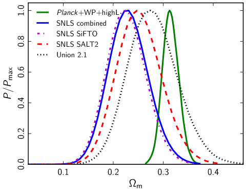
The results of this subsection are summarized in Fig. 19. This shows the posterior distributions for $\Omega_{\mathrm{m}}$ in the base $\Lambda$CDM cosmology, marginalized over nuisance parameters, for each of the SNe samples. These distributions are broad (with the Union2.1 distribution somewhat broader than the SNLS distributions) and show substantial overlap. There is no obvious inconsistency between the SNe samples. The posterior distribution for $\Omega_{\mathrm{m}}$ in the base $\Lambda$CDM model fit to Planck+WP+highL is shown by the narrow green curve. This is consistent with the Union2.1 and SNLS SALT2 results, but is in some tension with the distributions from the SNLS combined and SNLS SiFTO samples. As we will see in Sect. 6, Planck combined with Planck lensing and BAO measurements overwhelm SNe data for most of the extensions of the $\Lambda$CDM model considered in this paper. However, the results presented here suggest that there could be residual systematic errors in the SNe data that are not properly accounted for in the covariance matrices. Hints of new physics based on combining CMB and SNe data should therefore be treated with caution.

5.5 Additional data

In this subsection we review a number of other astrophysical data sets that have sometimes been combined with CMB data. These data sets are not used with Planck in this paper, either because they are statistically less powerful than the data reviewed in previous subsections and/or they involve complex physics (such as the behaviour of intra-cluster gas in rich clusters of galaxies) which is not yet well understood.

5.5.1 Shape information on the galaxy/matter power spectrum

Figure 20: Band-power estimates of the halo power spectrum, $P_{\rm halo}(k)$, from Reid et al. (2010) together with $1\thinspace\sigma$ errors. (Note that these data points are strongly correlated.) The line shows the predicted spectrum for the best-fit Planck+WP+highL base $\Lambda$CDM parameters.

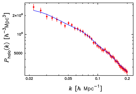
Reid et al. (2010) present an estimate of the dark matter halo power spectrum, $P_{\rm halo}(k)$, derived from $110{,}756$ luminous red galaxies (LRGs) from the SDSS 7th data release (Abazajian et al. 2009). The sample extends to redshifts $z\approx 0.5$, and is processed to identify LRGs occupying the same dark matter halo, reducing the impact of redshift-space distortions and recovering an approximation to the halo density field. The power spectrum $P_{\rm halo}(k)$ is reported in $45$ bands, covering the wavenumber range $0.02\thinspace h\thinspace{\rm Mpc}^{-1}<k<0.2\thinspace h\thinspace{\rm Mpc}^{-1}$. The window functions, covariance matrix and CosmoMC likelihood module are available on the NASA LAMBDA web site.

The halo power spectrum is plotted in Fig. 20. The blue line shows the predicted halo power spectrum from our best-fit base $\Lambda$CDM parameters convolved with the Reid et al. (2010) window functions. Here we show the predicted halo power spectrum for the best-fit values of the “nuisance” parameters $b_{0}$ (halo bias), $a_{1}$, and $a_{2}$ (defined in Eq. 15 of Reid et al. 2010) which relate the halo power spectrum to the dark matter power spectrum (computed using camb). The Planck model gives $\chi^{2}_{\rm LRG}=40.4$, very close to the value $\chi^{2}_{\rm LRG}=40.0$ of the best-fit model of Reid et al. (2010).

Figure 20 shows that the Planck parameters provide a good match to the shape of the halo power spectrum. However, we do not use these data (in this form) in conjunction with Planck. The BAO scale derived from these and other data is used with Planck, as summarized in Sect. 5.2. As discussed by Reid et al. (2010, see their figure 5) there is little additional information on cosmology once the BAO features are filtered from the spectrum, and hence little to be gained by adding this information to Planck. The corrections for nonlinear evolution, though small in the wavenumber range $0.1$–$0.2\thinspace h\thinspace{\rm Mpc}^{-1}$, add to the complexity of using shape information from the halo power spectrum.

5.5.2 Cosmic shear

Another key cosmological observable is the distortion of distant galaxy images by the gravitational lensing of large-scale structure, often called cosmic shear. The shear probes the (non-linear) matter density projected along the line of sight with a broad kernel. It is thus sensitive to the geometry of the Universe and the growth of large-scale structure, with a strong sensitivity to the amplitude of the matter power spectrum.

The most recent, and largest, cosmic shear data sets are provided by the CFHTLenS survey (Heymans et al. 2012; Erben et al. 2013), which covers $154\thinspace{\rm deg}^{2}$ in five optical bands with accurate shear measurements and photometric redshifts. The CFHTLenS team has released several cosmic shear results that are relevant to this paper. Benjamin et al. (2013) present results from a two-bin tomographic analysis and Heymans et al. (2013) from a finely binned tomographic analysis. Kilbinger et al. (2013) present constraints from a 2D analysis. The constraints from all of the analyses show a high degree of consistency.

Heymans et al. (2013) estimate shear correlation functions associated with six redshift bins. Assuming a flat, $\Lambda$CDM model, from the weak lensing data alone they find $\sigma_{8}\left(\Omega_{\rm m}/0.27\right)^{0.46\pm 0.02}=0.774\pm 0.04$ (68% errors) which is consistent with the constraint found by Benjamin et al. (2013). For comparison, we find

$$\sigma_{8}\left(\Omega_{\rm m}/0.27\right)^{0.46}=0.89\pm 0.03\quad\mbox{(68\%; {Planck}+WP+highL)},$$

(64)

which is discrepant at about the $2\thinspace\sigma$ level. Combining the tomographic lensing data with CMB constraints from WMAP-7, Heymans et al. (2013) are able to constrain the individual parameters of the flat, $\Lambda$CDM model to be $\Omega_{\rm m}=0.255\pm 0.014$ and $h=0.717\pm 0.016$. The best-fit Planck value of $\Omega_{\rm m}$ is $4\thinspace\sigma$ away from this value, while $h$ is discrepant at nearly $3\thinspace\sigma$. As might be expected, given the good agreement between the Planck and BAO distance scales, the best-fit CFHTLenS $\Lambda$CDM cosmology is also discrepant with the BOSS data, predicting a distance ratio to $z=0.57$ which is 5% lower than measured by BOSS (Anderson et al. 2012). This is discrepant at approximately the $3\thinspace\sigma$ level, comparable to the discrepancy with the Planck values. The source of the discrepancies between Planck and the CFHTLenS tomographic analyses is at present unclear, and further work will be needed to resolve them.

Kilbinger et al. (2013) give a tight constraint in the $\sigma_{8}$–$\Omega_{\rm m}$ plane for flat $\Lambda$CDM models from their 2D (i.e., non-tomographic) analysis. They find $\sigma_{8}\left(\Omega_{\rm m}/0.27\right)^{0.6}=0.79\pm 0.03$, which, when combined with WMAP-7, gives $\Omega_{\rm m}=0.283\pm 0.010$ and $h=0.69\pm 0.01$. These results are still discrepant with the Planck best-fit, but with lower significance than the results reported by Heymans et al. (2013).

It is also worth noting that a recent analysis of galaxy-galaxy lensing in the SDSS survey (Mandelbaum et al. 2013) leads to the constraint $\sigma_{8}\left(\Omega_{\rm m}/0.25\right)^{0.57}=0.80\pm 0.05$ for the base $\rm{\Lambda CDM}$ cosmology. This is about $2.4\thinspace\sigma$ lower than expected from Planck.

5.5.3 Counts of rich clusters

For the base $\Lambda$CDM model we find $\sigma_{8}=0.828\pm 0.012$ from Planck+WP+highL. This value is in excellent agreement with the WMAP-9 value of $\sigma_{8}=0.821\pm 0.023$ (Hinshaw et al. 2012). There are other ways to probe the power spectrum normalization, in addition to the cosmic shear measurements discussed above. For example, the abundances of rich clusters of galaxies are particularly sensitive to the normalization (see e.g., Komatsu & Seljak 2002). Recently, a number of studies have used tSZ-cluster mass scaling relations to constrain combinations of $\sigma_{8}$ and $\Omega_{\mathrm{m}}$ (e.g., Benson et al. 2013; Reichardt et al. 2013; Hasselfield et al. 2013) including an analysis of a sample of Planck tSZ clusters (see Planck Collaboration XXVIII 2014; Planck Collaboration XXIX 2014) reported in this series of papers (Planck Collaboration XX 2014).

The Planck analysis uses a relation between cluster mass and tSZ signal based on comparisons with X-ray mass measurements. To take into account departures from hydrostatic equilibrium, X-ray temperature calibration, modelling of the selection function, uncertainties in scaling relations and analysis uncertainties, Planck Collaboration XX (2014) assume a “bias” between the X-ray derived masses and the true cluster masses. If the mass bias, $(1-b)$, is allowed to vary uniformly between $0.7$ and $1.0$, Planck Collaboration XX (2014) find $\sigma_{8}(\Omega_{\mathrm{m}}/0.27)^{0.3}=0.76\pm 0.03$ for the base $\Lambda$CDM model. In comparison, for the same model we find

$$\sigma_{8}\left(\Omega_{\rm m}/0.27\right)^{0.3}=0.87\pm 0.02\quad\mbox{(68\%; {Planck}+WP+highL)},$$

(65)

which is a significant (around $3\thinspace\sigma$) discrepancy that remains unexplained. Qualitatively similar results are found from analyses of SPT clusters [$\sigma_{8}(\Omega_{\mathrm{m}}/0.27)^{0.3}=0.77\pm 0.04$]. Key difficulties with this type of measurement, as discussed in Planck Collaboration XX (2014), include adequately modelling selection biases and calibrating cluster masses. These effects are discussed in the analysis of ACT clusters by Hasselfield et al. (2013), who adopt a number of approaches, including folding in dynamical mass measurements, to calibrate biases in clusters mass estimates. Some of these approaches give joint $\sigma_{8}$–$\Omega_{\mathrm{m}}$ constraints consistent with the base $\Lambda$CDM parameters reported here.

At this stage of our understanding of the biases and scatter in the cluster mass calibrations, we believe that for the purposes of this paper it is premature to use cluster counts together with CMB measurements to search for new physics. Planck Collaboration XX (2014) explore a number of possibilities for reducing the tension between Planck  CMB measurements and tSZ cluster counts, including non-zero neutrino masses.

6 Extensions to the base $\rm{\Lambda CDM}$ model

6.1 Grid of models

Figure 21: 68% and 95% confidence regions on one-parameter extensions of the base $\rm{\Lambda CDM}$ model for Planck+WP (red) and Planck+WP+BAO (blue). Horizontal dashed lines correspond to the fixed base model parameter value, and vertical dashed lines show the mean posterior value in the base model for Planck+WP.

Table 10: Constraints on one-parameter extensions to the base $\Lambda$CDM model. Data combinations all include Planck combined with WMAP polarization, and results are shown for combinations with high-$\ell$ CMB data and BAO. Note that we quote 95% limits here.

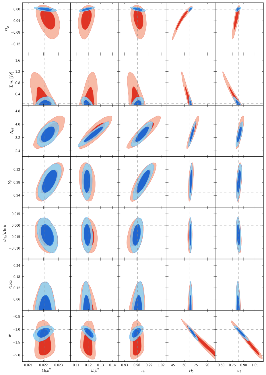
Planck+WP Planck+WP+BAO Planck+WP+highL Planck+WP+highL+BAO Parameter Best fit 95% limits Best fit 95% limits Best fit 95% limits Best fit 95% limits $$\Omega_{K} -0.0326 -0.037^{+0.043}_{-0.049} 0.0006 0.0000^{+0.0066}_{-0.0067} -0.0389 -0.042^{+0.043}_{-0.048} -0.0003 -0.0005^{+0.0065}_{-0.0066} \Sigma m_{\nu}\thinspace[\mathrm{eV}] 0.002 <0.933 0.000 <0.247 0.000 <0.663 0.001 <0.230 N_{\mathrm{eff}} 3.25 3.51^{+0.80}_{-0.74} 3.32 3.40^{+0.59}_{-0.57} 3.38 3.36^{+0.68}_{-0.64} 3.33 3.30^{+0.54}_{-0.51} Y_{\mathrm{P}} 0.2896 0.283^{+0.045}_{-0.048} 0.2889 0.283^{+0.043}_{-0.045} 0.2652 0.266^{+0.040}_{-0.042} 0.2701 0.267^{+0.038}_{-0.040} dn_{\mathrm{s}}/d\ln k -0.0125 -0.013^{+0.018}_{-0.018} -0.0097 -0.013^{+0.018}_{-0.018} -0.0146 -0.015^{+0.017}_{-0.017} -0.0143 -0.014^{+0.016}_{-0.017} r_{0.002} 0.000 <0.120 0.000 <0.122 0.000 <0.108 0.000 <0.111 w -1.94 -1.49^{+0.65}_{-0.57} -1.106 -1.13^{+0.24}_{-0.25} -1.94 -1.51^{+0.62}_{-0.53} -1.113 -1.13^{+0.23}_{-0.25}$$. . . . . . .  

To explore possible deviations from $\rm{\Lambda CDM}$ we have analysed an extensive grid of models that covers many well-motivated extensions of $\rm{\Lambda CDM}$. As in the exploration of the base $\rm{\Lambda CDM}$ cosmology, we have also considered a variety of data combinations for each model. For models involving more than one additional parameter we restrict ourselves to Planck+WP combinations in order to obtain tighter constraints by leveraging the relative amplitude of the power spectrum at very low $\ell$ and high $\ell$. Most models are run with Planck, Planck+WP, and Planck+WP+highL; additionally all are importance sampled with Planck lensing (Sect. 5.1), BAO (Sect. 5.2), SNe (Sect. 5.4), and the Riess et al. (2011) direct $H_{0}$ measurement (Sect. 5.3). For models where the non-CMB data give a large reduction in parameter volume (e.g. $\Omega_{K}$ models), we run separate chains instead of importance sampling.

These runs provide no compelling evidence for deviations from the base $\Lambda$CDM model, and indeed, as shown in Table 10 and Fig. 21, the posteriors for individual extra parameters generally overlap the fiducial model within one standard deviation. The inclusion of BAO data shrinks further the allowed scope for deviation. The parameters of the base $\rm{\Lambda CDM}$ model are relatively robust to inclusion of additional parameters, but the errors on some do broaden significantly when additional degeneracies open up, as can be seen in Fig. 21

The full grid results are available online. Here we summarize some of the key results, and also consider a few additional extensions.

6.2 Early-Universe physics

Inflationary cosmology offers elegant explanations of key features of our Universe, such as its large size and near spatially flat geometry. Within this scenario, the Universe underwent a brief period of accelerated expansion (Starobinsky 1979, 1982; Kazanas 1980; Guth 1981; Sato 1981; Linde 1982; Albrecht & Steinhardt 1982) during which quantum fluctuations were inflated in scale to become the classical fluctuations that we see today. In the simplest inflationary models, the primordial fluctuations are predicted to be adiabatic, nearly scale-invariant and Gaussian (Mukhanov & Chibisov 1981; Hawking 1982; Starobinsky 1982; Guth & Pi 1982; Bardeen et al. 1983), in good agreement with CMB observations and other probes of large-scale structure.

Despite this success, the fundamental physics behind inflation is not yet understood and there is no convincing evidence that rules out alternative scenarios for the early Universe. A large number of phenomenological models of inflation, some inspired by string theory, have been discussed in the literature (see Liddle & Lyth 2000; Bassett et al. 2006; Linde 2008, for reviews), as well as alternatives to inflation including pre-big bang scenarios (e.g., Gasperini & Veneziano 1993; Khoury et al. 2001; Boyle et al. 2004; Creminelli & Senatore 2007; Brandenberger 2012). Many of these models lead to distinctive signatures, such as departures from Gaussianity, isocurvature perturbations, or oscillatory features in the power spectrum, that are potentially observable. The detection of such signatures would offer valuable information on the physics of the early Universe and is one of the main science goals of Planck.

In this section we discuss basic aspects of the primordial power spectrum, such as the spectral index, departures from a pure power law, limits on tensor modes etc., and discuss the implications for inflationary cosmology. Tests of more complex models, such as multi-field inflation, are discussed in a separate paper (Planck Collaboration XXII 2014). In Planck Collaboration XXIV (2014), the Planck maps are used to constrain possible deviations from Gaussianity via measurements of the bispectrum and trispectrum. Planck Collaboration XXIII (2014) considers departures from statistical isotropy and additional tests of non-Gaussianity.

6.2.1 Scale dependence of primordial fluctuations

The primordial fluctuations in the base $\rm{\Lambda CDM}$ model are parameterized as a pure power law with a spectral index $n_{\rm s}$ (Eq. 2). Prior to Planck, CMB observations have favoured a power law index with slope $n_{\rm s}<1$, which is expected in simple single-field slow-roll inflationary models (see e.g., Mukhanov 2007 and Eq. 71a below). The final WMAP nine-year data give $n_{\rm s}=0.972\pm 0.013$ at 68% confidence (Hinshaw et al. 2012). Combining this with damping-tail measurements from ACT and SPT data gives $n_{\rm s}=0.968\pm 0.009$, indicating a departure from scale invariance at the 3$\thinspace\sigma$ level. The addition of BAO data has resulted in a stronger preference for $n_{\rm s}<1$ (Anderson et al. 2012; Hinshaw et al. 2012; Story et al. 2012; Sievers et al. 2013). These constraints assume the basic six-parameter $\rm{\Lambda CDM}$ cosmological model. Any new physics that affects the damping tail of the CMB spectrum, such as additional relativistic particles, can alter these constraints substantially and still allow a precisely scale-invariant spectrum.

With Planck, a robust detection of the deviation from scale invariance can now be made from a single set of CMB observations spanning three decades in scale from $\ell=2$ to $\ell=2500$. We find

$$n_{\rm s}=0.959\pm 0.007\quad\mbox{(68\%; {Planck}+WP+highL)},$$ (66)

for the base $\rm{\Lambda CDM}$ model, a roughly $6\thinspace\sigma$ departure from scale invariance. This is consistent with the results from previous CMB experiments cited above. The statistical significance of this result is high enough that the difference between a purely scale invariant spectrum can be seen easily in a plot of the power spectrum. Figure 22 shows the Planck spectrum of Fig. 10 plotted as $\ell^{2}{\cal D_{\ell}}$ compared to the base $\Lambda$CDM fit with $n_{\rm s}=0.96$ (red dashed line) and to the best-fit base $\Lambda$CDM cosmology with $n_{\rm s}=1$. The $n_{\rm s}=1$ model has more power at small scales and is strongly excluded by the Planck data.

Figure 22: The Planck power spectrum of Fig. 10 plotted as $\ell^{2}{\cal D_{\ell}}$ against multipole, compared to the best-fit base $\Lambda$CDM model with $n_{\rm s}=0.96$ (red dashed line). The best-fit base $\Lambda$CDM model with $n_{\rm s}$ constrained to unity is shown by the blue line.

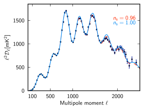
The unique contribution of Planck, compared to previous experiments, is that we are able to show that the departure from scale invariance is robust to changes in the underlying theoretical model. For example, Figs. 21 and 23 show that the departure from scale invariance is not sensitive to the parameterization of the primordial fluctuations. Even if we allow a possible running of the spectral index (the parameter $dn_{\rm s}/d\ln k$ defined in equation 2) and/or a component of tensor fluctuations, the Planck data favour a tilted spectrum at a high significance level.

Our extensive grid of models allows us to investigate correlations of the spectral index with a number of cosmological parameters beyond those of the base $\Lambda$CDM model (see Figs. 21 and 24). As expected, $n_{\rm s}$ is uncorrelated with parameters describing late-time physics, including the neutrino mass, geometry, and the equation of state of dark energy. The remaining correlations are with parameters that affect the evolution of the early Universe, including the number of relativistic species, or the helium fraction. This is illustrated in Fig. 24: modifying the standard model by increasing the number of neutrinos species, or the helium fraction, has the effect of damping the small-scale power spectrum. This can be partially compensated by an increase in the spectral index. However, an increase in the neutrino species must be accompanied by an increased matter density to maintain the peak positions. A measurement of the matter density from the BAO measurements helps to break this degeneracy. This is clearly seen in the upper panel of Fig. 24, which shows the improvement in the constraints when BAO measurements are added to the Planck+WP+highL likelihood. With the addition of BAO measurements we find more than a 3$\thinspace\sigma$ deviation from $n_{\rm s}=1$ even in this extended model, with a best-fit value of $n_{\rm s}=0.969\pm 0.010$ for varying relativistic species. As discussed in Sect. 6.3, we see no evidence from the Planck data for non-standard neutrino physics.

Figure 23: Upper: Posterior distribution for $n_{\rm s}$ for the base $\Lambda$CDM model (black) compared to the posterior when a tensor component and running scalar spectral index are added to the model (red) Middle: Constraints (68% and 95%) in the $n_{\rm s}$–$dn_{\rm s}/d\ln k$ plane for $\Lambda$CDM models with running (blue) and additionally with tensors (red). Lower: Constraints (68% and 95%) on $n_{\rm s}$ and the tensor-to-scalar ratio $r_{0.002}$ for $\Lambda$CDM models with tensors (blue) and additionally with running of the spectral index (red). The dotted line show the expected relation between $r$ and $n_{\rm s}$ for a $V(\phi)\propto\phi^{2}$ inflationary potential (Eqs. 71a and 71b); here $N$ is the number of inflationary e-foldings as defined in the text. The dotted line should be compared to the blue contours, since this model predicts negligible running. All of these results use the Planck+WP+highL data combination.

Figure 24: Constraints on $n_{\rm s}$ for $\Lambda$CDM models with non-standard relativistic species, $N_{\rm eff}$, (upper) and helium fraction, $Y_{\text{P}}$, (lower). We show 68% and 95% contours for various data combinations. Note the tightening of the constraints with the addition of BAO data.

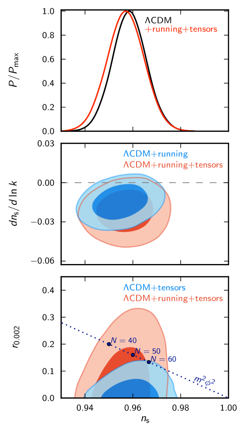
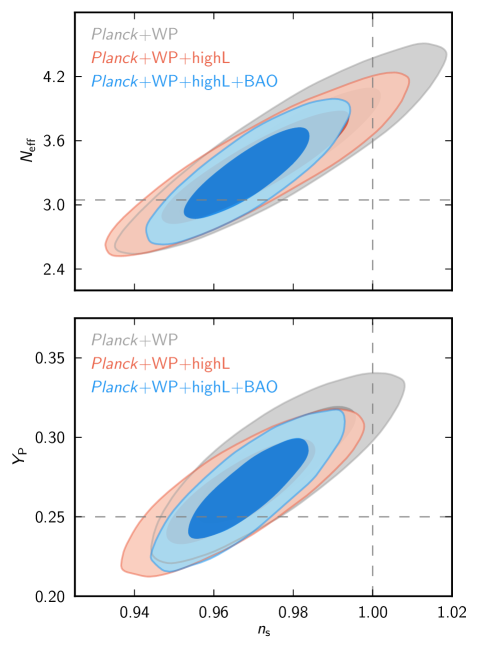
The simplest single-field inflationary models predict that the running of the spectral index should be of second order in inflationary slow-roll parameters and therefore small [$dn_{\rm s}/d\ln k\sim(n_{\rm s}-1)^{2}$], typically about an order of magnitude below the sensitivity limit of Planck (see e.g., Kosowsky & Turner 1995; Baumann et al. 2009). Nevertheless, it is easy to construct inflationary models that have a larger scale dependence (e.g., by adjusting the third derivative of the inflaton potential) and so it is instructive to use the Planck data to constrain $dn_{\rm s}/d\ln k$. A test for $dn_{\rm s}/d\ln k$ is of particularly interest given the results from previous CMB experiments.

Early results from WMAP suggested a preference for a negative running at the 1–2$\thinspace\sigma$ level. In the final 9-year WMAP analysis no significant running was seen using WMAP data alone, with $dn_{\rm s}/d\ln k=-0.019\pm 0.025$ (68% confidence; Hinshaw et al. 2012. Combining WMAP data with the first data releases from ACT and SPT, Hinshaw et al. (2012) found a negative running at nearly the $2\thinspace\sigma$ level with $dn_{\rm s}/d\ln k=-0.022\pm 0.012$ (see also Dunkley et al. 2011 and Keisler et al. 2011 for analysis of ACT and SPT with earlier data from WMAP). The ACT 3-year release, which incorporated a new region of sky, gave $dn_{\rm s}/d\ln k=-0.003\pm 0.013$ (Sievers et al. 2013) when combined with WMAP 7 year data. With the wide field SPT data at 150 GHz, a negative running was seen at just over the $2\thinspace\sigma$ level, $dn_{\rm s}/d\ln k=-0.024\pm 0.011$ (Hou et al. 2012).

The picture from previous CMB experiments is therefore mixed. The latest WMAP data show a $1\thinspace\sigma$ trend for a running, but when combined with the S12 SPT data, this trend is amplified to give a potentially interesting result. The latest ACT data go in the other direction, giving no support for a running spectral index when combined with WMAP.

The results from Planck data are as follows (see Figs. 21 and 23):

$$dn_{\rm s}/d\ln k = -0.013\pm 0.009\;\mbox{(68\%; {Planck}+WP)};$$ (67a)

$$dn_{\rm s}/d\ln k = -0.015\pm 0.009\;\mbox{(68\%; {Planck}+WP+highL)};$$ (67b)

$$dn_{\rm s}/d\ln k = -0.011\pm 0.008\;\mbox{(68\%; {Planck}+lensing}$$ (67c)

$$\hskip 116.6563pt\mbox{+WP+highL)}.$$

The consistency between (67a) and (67b) shows that these results are insensitive to modelling of unresolved foregrounds. The preferred solutions have a small negative running, but not at a high level of statistical significance. Closer inspection of the best-fits shows that the change in $\chi^{2}$ when $dn_{\rm s}/d\ln k$ is included as a parameter comes almost entirely from the low multipole temperature likelihood. (The fits to the high multipole Planck likelihood have a $\Delta\chi^{2}=-0.4$ when $dn_{\rm s}/d\ln k$ is included.) The slight preference for a negative running is therefore driven by the spectrum at low multipoles $\ell\la 50$. The tendency for negative running is partly mitigated by including the Planck lensing likelihood (Eq. 67c).

The constraints on $dn_{\rm s}/d\ln k$ are broadly similar if tensor fluctuations are allowed in addition to a running of the spectrum (Fig. 23) . Adding tensor fluctuations, the marginalized posterior distributions for $dn_{\rm s}/d\ln k$ give

$$dn_{\rm s}/d\ln k = -0.021\pm 0.011\;\mbox{(68\%; {Planck}+WP)},$$ (68a)

$$dn_{\rm s}/d\ln k = -0.022\pm 0.010\;\mbox{(68\%; {Planck}+WP+highL)},$$ (68b)

$$dn_{\rm s}/d\ln k = -0.019\pm 0.010\;\mbox{(68\%; {Planck}+lensing}$$ (68c)

$$\hskip 116.6563pt\mbox{+WP+highL)}.$$

As with Eqs. (67a)–(67c) the tendency to favour negative running is driven by the low multipole component of the temperature likelihood not by the Planck spectrum at high multipoles.

This is one of several examples discussed in this section where marginal evidence for extensions to the base $\Lambda$CDM model are favoured by the $TT$ spectrum at low multipoles. (The low multipole spectrum is also largely responsible for the pull of the lensing amplitude, $A_{\rm L}$, to values greater than unity discussed in Sect. 5.1). The mismatch between the best-fit base $\Lambda$CDM model and the $TT$ spectrum at multipoles $\ell\la 30$ is clearly visible in Fig. 1. The implications of this mismatch are discussed further in Sect. 7.

Beyond a simple running, various extended parameterizations have been developed by e.g., Bridle et al. (2003), Shafieloo & Souradeep (2008), Verde & Peiris (2008), and Hlozek et al. (2012), to test for deviations from a power-law spectrum of fluctuations. Similar techniques are applied to the Planck data in  Planck Collaboration XXII (2014).

6.2.2 Tensor fluctuations

In the base $\rm{\Lambda CDM}$ model, the fluctuations are assumed to be purely scalar modes. Primordial tensor fluctuations could also contribute to the temperature and polarization power spectra (e.g., Grishchuk 1975; Starobinsky 1979; Basko & Polnarev 1980; Crittenden et al. 1993, 1995). The most direct way of testing for a tensor contribution is to search for a magnetic-type parity signature via a large-scale $B$-mode pattern in CMB polarization (Seljak 1997; Zaldarriaga & Seljak 1997; Kamionkowski et al. 1997). Direct $B$-mode measurements are challenging as the expected signal is small; upper limits measured by BICEP and QUIET give $95\%$ upper limits of $r_{0.002}<0.73$ and $r_{0.002}<2.8$ respectively (Chiang et al. 2010; QUIET Collaboration et al. 2012).

Measurements of the temperature power spectrum can also be used to constrain the amplitude of tensor modes. Although such limits can appear to be much tighter than the limits from $B$-mode measurements, it should be borne in mind that such limits are indirect because they are derived within the context of a particular theoretical model. In the rest of this subsection, we will review temperature based limits on tensor modes and then present the results from Planck.

Adding a tensor component to the base $\rm{\Lambda CDM}$ model, the WMAP 9-year results constrain $r_{0.002}<0.38$ at 95% confidence (Hinshaw et al. 2012). Including small-scale ACT and SPT data this improves to $r_{0.002}<0.17$, and to $r_{0.002}<0.12$ with the addition of BAO data. These limits are degraded substantially, however, in models which allow running of the scalar spectral index in addition to tensors. For such models, the WMAP data give $r_{0.002}<0.50$, and this limit is not significantly improved by adding high resolution CMB and BAO data.

The precise determination of the fourth, fifth and sixth acoustic peaks by Planck now largely breaks the degeneracy between the primordial fluctuation parameters. For the Planck+WP+highL likelihood we find

$$r_{0.002} < 0.11\quad\mbox{(95\%; no running)},$$ (69a)

$$r_{0.002} < 0.26\quad\mbox{(95\%; including running)}.$$ (69b)

As shown in Figs. 21 and 23, the tensor amplitude is weakly correlated with the scalar spectral index; an increase in $n_{\rm s}$ that could match the first three peaks cannot fit the fourth and higher acoustic peak in the Planck spectrum. Likewise, the shape constraints from the fourth and higher acoustic peaks give a reduction in the correlations between a tensor mode and a running in the spectral index, leading to significantly tighter limits than from previous CMB experiments. These numbers in Eqs. (69a) and (69b) are driven by the temperature spectrum and change very little if we add non-CMB data such as BAO measurements. The Planck limits are largely decoupled from assumptions about the late-time evolution of the Universe and are close to the tightest possible limits achievable from the temperature power spectrum alone (Knox & Turner 1994; Knox 1995).

These limits on a tensor mode have profound implications for inflationary cosmology. The limits translate directly to an upper limit on the energy scale of inflation,

$$V_{*}=(1.94\times 10^{16}\ {\rm GeV})^{4}(r_{0.002}/0.12)$$ (70)

(Linde 1983; Lyth 1984), and to the parameters of “large-field” inflation models. Slow-roll inflation driven by a power law potential $V(\phi)\propto\phi^{\alpha}$ offers a simple example of large-field inflation. The field values in such a model must necessarily exceed the Planck scale $m_{\rm Pl}$ , and lead to a scalar spectral index and tensor amplitude of

$$1-n_{\rm s} \approx (\alpha+2)/2N,$$ (71a)

$$r \approx 4\alpha/N,$$ (71b)

where $N$ is the number of e-foldings between the end of inflation and the time that our present day Hubble scale crossed the inflationary horizon (see e.g., Lyth & Riotto 1999). The 95% confidence limits from the Planck data are now close to the predictions of $\alpha=2$ models for $N\approx 50$–60 e-folds (see Fig. 23). Large-field models with quartic potentials (e.g., Linde 1982) are now firmly excluded by CMB data. Planck constraints on power-law and on broader classes of inflationary models are discussed in detail in Planck Collaboration XXIV (2014). Improved limits on $B$-modes will be required to further constrain high field models of inflation.

Figure 25: The Planck+WP+highL data combination (samples; colour-coded by the value of $H_{0}$) partially breaks the geometric degeneracy between $\Omega_{\rm m}$ and $\Omega_{\Lambda}$ due to the effect of lensing in the temperature power spectrum. These limits are significantly improved by the inclusion of the Planck lensing reconstruction (black contours). Combining also with BAO (right; solid blue contours) tightly constrains the geometry to be nearly flat.

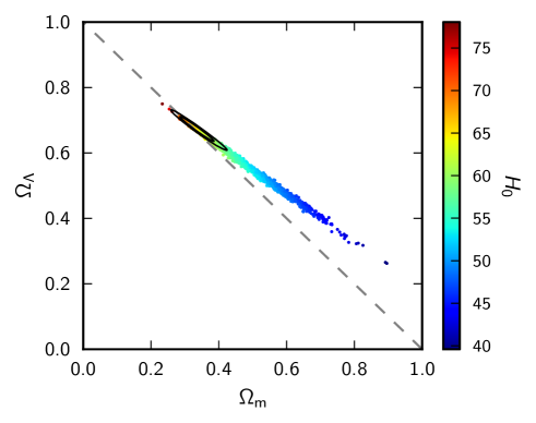
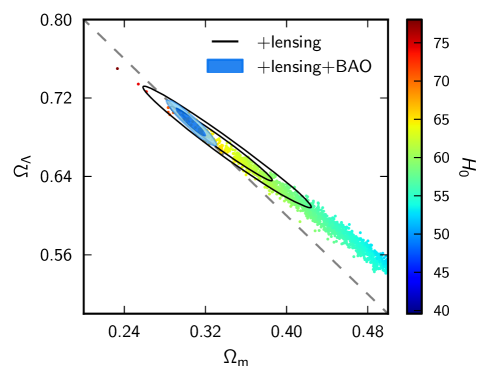
6.2.3 Curvature

An explanation of the near flatness of our observed Universe was one of the primary motivations for inflationary cosmology. Inflationary models that allow a large number of e-foldings predict that our Universe should be very accurately spatially flat. Nevertheless, by introducing fine tunings it is possible to construct inflation models with observationally interesting open geometries (e.g., Gott 1982; Linde 1995; Bucher et al. 1995; Linde 1999) or closed geometries (Linde 2003). Even more speculatively, there has been interest in models with open geometries from considerations of tunnelling events between metastable vacua within a “string landscape” (Freivogel et al. 2006). Observational limits on spatial curvature therefore offer important additional constraints on inflationary models and fundamental physics.

CMB temperature power spectrum measurements suffer from a well-known “geometrical degeneracy” (Bond et al. 1997; Zaldarriaga et al. 1997). Models with identical primordial spectra, physical matter densities and angular diameter distance to the last scattering surface, will have almost identical CMB temperature power spectra. This is a near perfect degeneracy (see Fig. 25) and is broken only via the integrated Sachs-Wolfe (ISW) effect on large angular scales and gravitational lensing of the CMB spectrum (Stompor & Efstathiou 1999). The geometrical degeneracy can also be broken with the addition of probes of late time physics, including BAO, Type Ia supernova, and measurement of the Hubble constant (e.g., Spergel et al. 2007).

Recently, the detection of the gravitational lensing of the CMB by ACT and SPT has been used to break the geometrical degeneracy, by measuring the integrated matter potential distribution. ACT constrained $\Omega_{\Lambda}=0.61\pm 0.29$ (68% CL) in Sherwin et al. (2011), with the updated analysis in Das et al. (2013) giving $\Omega_{K}=-0.031\pm 0.026$ (68% CL) (Sievers et al. 2013). The SPT lensing measurements combined with seven year WMAP temperature spectrum improved this limit to $\Omega_{K}=-0.0014\pm 0.017$ (68 % CL) (van Engelen et al. 2012).

With Planck we detect gravitational lensing at about $26\thinspace\sigma$ through the 4-point function (Sect. 5.1 and Planck Collaboration XVII 2014). This strong detection of gravitational lensing allows us to constrain the curvature to percent level precision using observations of the CMB alone:

$$100\Omega_{K} = -4.2^{+4.3}_{-4.8}\quad\mbox{(95\%; {Planck}+WP+highL});$$ (72a)

$$100\Omega_{K} = -1.0^{+1.8}_{-1.9}\quad\mbox{(95\%; {Planck}+lensing}$$ (72b)

$$\hskip 125.19212pt\mbox{+ WP+highL)}.$$

These constraints are improved substantially by the addition of BAO data. We then find

$$100\Omega_{K} = -0.05^{+0.65}_{-0.66}\ \ \mbox{(95\%; {Planck}+WP+highL+BAO}),$$ (73a)

$$100\Omega_{K} = -0.10^{+0.62}_{-0.65}\quad\mbox{(95\%; {Planck}+lensing+WP}$$ (73b)

$$\qquad\qquad\qquad\qquad\qquad\quad\quad\mbox{+highL+BAO)}.$$

These limits are consistent with (and slightly tighter than) the results reported by Hinshaw et al. (2012) from combining the nine-year WMAP data with high resolution CMB measurements and BAO data. We find broadly similar results to Eqs. (73a) and (73b) if the Riess et al. (2011) $H_{0}$ measurement, or either of the SNe compilations discussed in Sect. 5.4, are used in place of the BAO measurements.

In summary, there is no evidence from Planck for any departure from a spatially flat geometry. The results of Eqs. (73a) and (73b) suggest that our Universe is spatially flat to an accuracy of better than a percent.

6.3 Neutrino physics and constraints on relativistic components

A striking illustration of the interplay between cosmology and particle physics is the potential of CMB observations to constrain the properties of relic neutrinos, and possibly of additional light relic particles in the Universe (see e.g., Dodelson et al. 1996; Hu et al. 1995; Bashinsky & Seljak 2004; Ichikawa et al. 2005; Lesgourgues & Pastor 2006; Hannestad 2010). In the following subsections, we present Planck constraints on the mass of ordinary (active) neutrinos assuming no extra relics, on the density of light relics assuming they all have negligible masses, and finally on models with both light massive and massless relics.

6.3.1 Constraints on the total mass of active neutrinos

The detection of solar and atmospheric neutrino oscillations proves that neutrinos are massive, with at least two species being non-relativistic today. The measurement of the absolute neutrino mass scale is a challenge for both experimental particle physics and observational cosmology. The combination of CMB, large-scale structure and distance measurements already excludes a large range of masses compared to beta-decay experiments. Current limits on the total neutrino mass $\sum m_{\nu}$ (summed over the three neutrino families) from cosmology are rather model dependent and vary strongly with the data combination adopted. The tightest constraints for flat models with three families of neutrinos are typically around $0.3\thinspace\mathrm{eV}$ (95% CL; e.g., de Putter et al. 2012). Since $\sum m_{\nu}$ must be greater than approximately $0.06\thinspace\mathrm{eV}$ in the normal hierarchy scenario and $0.1\thinspace\mathrm{eV}$ in the degenerate hierarchy (Gonzalez-Garcia et al. 2012), the allowed neutrino mass window is already quite tight and could be closed further by current or forthcoming observations (Jimenez et al. 2010; Lesgourgues et al. 2013).

Cosmological models, with and without neutrino mass, have different primary CMB power spectra. For observationally-relevant masses, neutrinos are still relativistic at recombination and the unique effects of masses in the primary power spectra are small. The main effect is around the first acoustic peak and is due to the early integrated Sachs-Wolfe (ISW) effect; neutrino masses have an impact here even for a fixed redshift of matter–radiation equality (Lesgourgues & Pastor 2012; Hall & Challinor 2012; Hou et al. 2012; Lesgourgues et al. 2013). To date, this effect has been the dominant one in constraining the neutrino mass from CMB data, as demonstrated in Hou et al. (2012). As we shall see here, the Planck data move us into a new regime where the dominant effect is from gravitational lensing. Increasing neutrino mass, while adjusting other parameters to remain in a high-probability region of parameter space, increases the expansion rate at $z\ga 1$ and so suppresses clustering on scales smaller than the horizon size at the non-relativistic transition (Kaplinghat et al. 2003; Lesgourgues et al. 2006). The net effect for lensing is a suppression of the CMB lensing potential and, for orientation, by $\ell=1000$ the suppression is around $10\%$ in power for $\sum m_{\nu}=0.66\thinspace\mathrm{eV}$.

Here we report constraints assuming three species of degenerate massive neutrinos. At the level of sensitivity of Planck, the effect of mass splittings is negligible, and the degenerate model can be assumed without loss of generality.

Figure 26: Marginalized posterior distributions for $\sum m_{\nu}$ in flat models from CMB data. We show results for Planck+WP+highL without (solid black) and with (red) marginalization over $A_{\rm L}$, showing how the posterior is significantly broadened by removing the lensing information from the temperature anisotropy power spectrum. The effect of replacing the low-$\ell$ temperature and (WMAP) polarization data with a $\tau$ prior is shown in solid blue (Planck$-$lowL+highL+$\tau$prior) and of further removing the high-$\ell$ data in dot-dashed blue (Planck$-$lowL+$\tau$prior). We also show the result of including the lensing likelihood with Planck+WP+highL (dashed black) and Planck$-$lowL+highL+$\tau$prior (dashed blue).

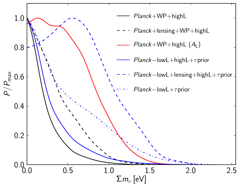
Combining the Planck+WP+highL data, we obtain an upper limit on the summed neutrino mass of

$$\sum m_{\nu}<0.66\thinspace\mathrm{eV}\quad\mbox{(95\%; {Planck}+WP+highL)}.$$ (74)

The posterior distribution is shown by the solid black curve in Fig. 26. To demonstrate that the dominant effect leading to the constraint is gravitational lensing, we remove the lensing information by marginalizing over $A_{\rm L}$. We see that the posterior broadens considerably (see the red curve in Fig. 26) to give

$$\sum m_{\nu}<1.08\thinspace\mathrm{eV}\quad\mbox{[95\%; {Planck}+WP+highL\ ($A_{\rm L}$)]},$$ (75)

taking us back close to the value of $1.3\thinspace\mathrm{eV}$ (for $A_{\rm L}=1$) from the nine-year WMAP data (Hinshaw et al. 2012), corresponding to the limit above which neutrinos become non-relativistic before recombination. (The resolution of WMAP gives very little sensitivity to lensing effects.)

As discussed in Sect. 5.1, the Planck+WP+highL data combination has a preference for high $A_{\rm L}$. Since massive neutrinos suppress the lensing power (like a low $A_{\rm L}$) there is a concern that the same tensions which drive $A_{\rm L}$ high may give artificially tight constraints on $\sum m_{\nu}$. We can investigate this issue by replacing the low-$\ell$ data with a prior on the optical depth (as in Sect. 5.1) and removing the high-$\ell$ data. Posterior distributions with the $\tau$ prior, and additionally without the high-$\ell$ data, are shown in Fig. 26 by the solid blue and dot-dashed blue curves, respectively. The constraint on $\sum m_{\nu}$ does not degrade much by replacing the low-$\ell$ data with the $\tau$ prior only, but the degradation is more severe when the high-$\ell$ data are also removed: $\sum m_{\nu}<1.31\thinspace\mathrm{eV}$ (95% CL).

Including the lensing likelihood (see Sect. 5.1) has a significant, but surprising, effect on our results. Adding the lensing likelihood to the Planck+WP+highL data combination weakens the limit on $\sum m_{\nu}$,

$$\sum m_{\nu}<0.85\thinspace\mathrm{eV}\quad\mbox{(95\%; {Planck}+lensing+WP+highL)},$$ (76)

as shown by the dashed black curve in Fig. 26. This is representative of a general trend that the Planck lensing likelihood favours larger $\sum m_{\nu}$ than the temperature power spectrum. Indeed, if we use the data combination Planck$-$lowL+highL+$\tau$prior, which gives a weaker constraint from the temperature power spectrum, adding lensing gives a best-fit away from zero ($\sum m_{\nu}=0.46\thinspace\mathrm{eV}$; dashed blue curve in Fig. 26). However, the total $\chi^{2}$ at the best-fit is very close to that for the best-fitting base model (which, recall, has one massive neutrino of mass $0.06\thinspace{\rm eV}$), with the improved fit to the lensing data ($\Delta\chi^{2}=-2.35$) being cancelled by the poorer fit to high-$\ell$ CMB data ($\Delta\chi^{2}=-2.15$). There are rather large shifts in other cosmological parameters between these best-fit solutions corresponding to shifts along the acoustic-scale degeneracy direction for the temperature power spectrum. Note that, as well as the change in $H_{0}$ (which falls to compensate the increase in $\sum m_{\nu}$ at fixed acoustic scale), $n_{\rm s}$, $\omega_{\mathrm{b}}$ and $\omega_{\mathrm{c}}$ change significantly keeping the lensed temperature spectrum almost constant. These latter shifts are similar to those discussed for $A_{\rm L}$ in Sect. 5.1, with non-zero $\sum m_{\nu}$ acting like $A_{\rm L}<1$. The lensing power spectrum $C_{\ell}^{\phi\phi}$ is lower by $5.4\%$ for the higher-mass best fit at $\ell=400$ and larger below $\ell\approx 45$ (e.g. by $0.6\%$ at $\ell=40$), which is a similar trend to the residuals from the best-fit minimal-mass model shown in the bottom panel of Fig. 12. Planck Collaboration XVII (2014) explores the robustness of the $C_{\ell}^{\phi\phi}$ estimates to various data cuts and foreground-cleaning methods. The first ($\ell=40$–$85$) bandpower is the least stable to these choices, although the variations are not statistically significant. We have checked that excluding this bandpower does not change the posterior for $\sum m_{\nu}$ significantly, as expected since most of the constraining power on $\sum m_{\nu}$ comes from the bandpowers on smaller scales. At this stage, it is unclear what to make of this mild preference for high masses from the 4-point function compared to the 2-point function. As noted in Planck Collaboration XVII (2014), the lensing measurements from ACT (Das et al. 2013) and SPT (van Engelen et al. 2012) show similar trends to those from Planck where they overlap in scale. With further Planck data (including polarization), and forthcoming measurements from the full $2500\thinspace\mathrm{deg}^{2}$ SPT temperature survey, we can expect more definitive results on this issue in the near future.

Apart from its impact on the early-ISW effect and lensing potential, the total neutrino mass affects the angular-diameter distance to last scattering, and can be constrained through the angular scale of the first acoustic peak. However, this effect is degenerate with $\Omega_{\Lambda}$ (and so the derived $H_{0}$) in flat models and with other late-time parameters such as $\Omega_{K}$ and $w$ in more general models (Howlett et al. 2012). Late-time geometric measurements help in reducing this “geometric” degeneracy. Increasing the neutrino masses at fixed $\theta_{\ast}$ increases the angular-diameter distance for $0\leq z\leq z_{\ast}$ and reduces the expansion rate at low redshift ($z\la 1$) but increases it at higher redshift. The spherically-averaged BAO distance $D_{\rm V}(z)$ therefore increases with increasing neutrino mass at fixed $\theta_{\ast}$, and the Hubble constant falls; see Fig. 8 of Hou et al. (2012). With the BAO data of Sect. 5.2, we find a significantly lower bound on the neutrino mass:

$$\sum m_{\nu}<0.23\thinspace\mathrm{eV}\quad\mbox{(95\%; {Planck}+WP+highL+BAO)}.$$ (77)

Following the philosophy of this paper, namely to give higher weight to the BAO data compared to more complex astrophysical data, we quote the result of Eq. (77) in the abstract as our most reliable limit on the neutrino mass. The $\Lambda$CDM model with minimal neutrino masses was shown in Sect. 5.3 to be in tension with recent direct measurements of $H_{0}$ which favour higher values. Increasing the neutrino mass will only make this tension worse and drive us to artificially tight constraints on $\sum m_{\nu}$. If we relax spatial flatness, the CMB geometric degeneracy becomes three-dimensional in models with massive neutrinos and the constraints on $\sum m_{\nu}$ weaken considerably to

$$\sum m_{\nu}<\left\{\begin{tabular}[]{ll}$0.98\thinspace\mathrm{eV}$&\mbox{(95\%; {Planck}+WP+highL)}\\ $0.32\thinspace\mathrm{eV}$&\mbox{(95\%; {Planck}+WP+highL+BAO}).\end{tabular}\right.$$ (78)

6.3.2 Constraints on $N_{\rm eff}$

As discussed in Sect. 2, the density of radiation in the Universe (besides photons) is usually parameterized by the effective neutrino number $N_{\rm eff}$. This parameter specifies the energy density when the species are relativistic in terms of the neutrino temperature assuming exactly three flavours and instantaneous decoupling. In the Standard Model, $N_{\rm eff}=3.046$, due to non-instantaneous decoupling corrections (Mangano et al. 2005).

However, there has been some mild preference for $N_{\rm eff}>3.046$ from recent CMB anisotropy measurements (Komatsu et al. 2011; Dunkley et al. 2011; Keisler et al. 2011; Archidiacono et al. 2011; Hinshaw et al. 2012; Hou et al. 2012). This is potentially interesting, since an excess could be caused by a neutrino/anti-neutrino asymmetry, sterile neutrinos, and/or any other light relics in the Universe. In this subsection we discuss the constraints on $N_{\rm eff}$ from Planck in scenarios where the extra relativistic degrees of freedom are effectively massless.

The physics of how $N_{\rm eff}$ is constrained by CMB anisotropies is explained in Bashinsky & Seljak (2004), Hou et al. (2011) and Lesgourgues et al. (2013). The main effect is that increasing the radiation density at fixed $\theta_{\ast}$ (to preserve the angular scales of the acoustic peaks) and fixed $z_{\text{eq}}$ (to preserve the early-ISW effect and so first-peak height) increases the expansion rate before recombination and reduces the age of the Universe at recombination. Since the diffusion length scales approximately as the square root of the age, while the sound horizon varies proportionately with the age, the angular scale of the photon diffusion length, $\theta_{\rm D}$, increases, thereby reducing power in the damping tail at a given multipole. Combining Planck, WMAP polarization and the high-$\ell$ experiments gives

$$N_{\rm eff}=3.36_{-0.64}^{+0.68}\quad\mbox{(95\%; {Planck}+WP+highL)}.$$ (79)

The marginalized posterior distribution is given in Fig. 27 (black curve). The result in Eq. (79) is consistent with the value of $N_{\rm eff}=3.046$ of the Standard Model, but it is important to aknowledge that it is difficult to constrain $N_{\rm eff}$ accurately using CMB temperature measurements alone. Evidently, the nominal mission data from Planck do not strongly rule out a value as high as $N_{\rm eff}=4$.

Figure 27: Marginalized posterior distribution of $N_{\rm eff}$ for Planck+WP+highL (black) and additionally BAO (blue), the $H_{0}$ measurement (red), and both BAO and $H_{0}$ (green).

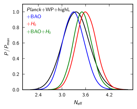
Increasing $N_{\rm eff}$ at fixed $\theta_{\ast}$ and $z_{\text{eq}}$ necessarily raises the expansion rate at low redshifts too. Combining CMB with distance measurements can therefore improve constraints (see Fig. 27) although for the BAO observable $r_{\rm drag}/D_{\rm V}(z)$ the reduction in both $r_{\rm drag}$ and $D_{\rm V}(z)$ with increasing $N_{\rm eff}$ partly cancel. With the BAO data of Sect. 5.2, the $N_{\rm eff}$ constraint is tightened to

$$N_{\rm eff}=3.30_{-0.51}^{+0.54}\quad\mbox{(95\%; {Planck}+WP+highL+BAO)}.$$ (80)

Our constraints from CMB alone and CMB+BAO are compatible with the standard value $N_{\rm eff}=3.046$ at the $1\thinspace\sigma$ level, giving no evidence for extra relativistic degrees of freedom.

Since $N_{\rm eff}$ is positively correlated with $H_{0}$, the tension between the Planck data and direct measurements of $H_{0}$ in the base $\Lambda$CDM model (Sect. 5.3) can be reduced at the expense of high $N_{\rm eff}$. The marginalized constraint is

$$N_{\rm eff}=3.62_{-0.48}^{+0.50}\quad\mbox{(95\%; {Planck}+WP+highL+$H_{0}$)}.$$ (81)

For this data combination, the $\chi^{2}$ for the best-fitting model allowing $N_{\rm eff}$ to vary is lower by $5.3$ than for the base $N_{\rm eff}=3.046$ model. The $H_{0}$ fit is much better, with $\Delta\chi^{2}=-4.4$, but there is no strong preference either way from the CMB. The low-$\ell$ temperature power spectrum does weakly favour the high $N_{\rm eff}$ model ($\Delta\chi^{2}=-1.4$) – since $N_{\rm eff}$ is positively correlated with $n_{\rm s}$ (see Fig. 24) and increasing $n_{\rm s}$ reduces power on large scales – as does the rest of the Planck power spectrum ($\Delta\chi^{2}=-1.8$). The high-$\ell$ experiments mildly disfavour high $N_{\rm eff}$ in our fits ($\Delta\chi^{2}=1.9$). Further including the BAO data pulls the central value downwards by around $0.5\thinspace\sigma$ (see Fig. 27):

$$N_{\rm eff}=3.52_{-0.45}^{+0.48}\quad\mbox{(95\%; {Planck}+WP+highL+$H_{0}$+BAO)}.$$ (82)

The $\chi^{2}$ at the best-fit for this data combination ($N_{\rm eff}=3.48$) is lower by $4.2$ than the best-fitting $N_{\rm eff}=3.046$ model. While the high $N_{\rm eff}$ best-fit is preferred by Planck+WP ($\Delta\chi^{2}=-3.1$) and the $H_{0}$ data ($\Delta\chi^{2}=-3.3$ giving an acceptable $\chi^{2}=1.8$ for this data point), it is disfavoured by the high-$\ell$ CMB data ($\Delta\chi^{2}=2.0$) and slightly by BAO ($\Delta\chi^{2}=0.5$). We conclude that the tension between direct $H_{0}$ measurements and the CMB and BAO data in the base $\Lambda$CDM can be relieved at the cost of additional neutrino-like physics, but there is no strong preference for this extension from the CMB damping tail.

Throughout this subsection, we have assumed that all the relativistic components parameterized by $N_{\rm eff}$ consist of ordinary free-streaming relativistic particles. Extra radiation components with a different sound speed or viscosity parameter (Hu 1998) can provide a good fit to pre-Planck CMB data (Archidiacono et al. 2013), but are not investigated in this paper.

6.3.3 Simultaneous constraints on $N_{\rm eff}$ and either $\sum m_{\nu}$ or $m_{\nu,\thinspace\mathrm{sterile}}^{\mathrm{eff}}$

It is interesting to investigate simultaneous contraints on $N_{\rm eff}$ and $\sum m_{\nu}$, since extra relics could coexist with neutrinos of sizeable mass, or could themselves have a mass in the eV range. Joint constraints on $N_{\rm eff}$ and $\sum m_{\nu}$ have been explored several times in the literature. These two parameters are known to be partially degenerate when large-scale structure data are used (Hannestad & Raffelt 2004; Crotty et al. 2004), but their impact in the CMB is different and does not lead to significant correlations.

Joint constraints on $N_{\rm eff}$ and $\sum m_{\nu}$ are always model-dependent: they vary strongly with assumptions about how the total mass is split between different species (and they would also be different for models in which massive species have chemical potentials or a non-thermal phase-space distribution). We present here Planck constraints for two different models and describe the scenarios that motivate them.

First, as in the previous subsection we assume that the three active neutrinos share a mass of $\sum m_{\nu}/3$, and may coexist with extra massless species contributing to $N_{\rm eff}$. In this model, when $N_{\rm eff}$ is greater than 3.046, $\Delta N_{\rm eff}=N_{\rm eff}-3.046$ gives the density of extra massless relics with arbitrary phase-space distribution. When $N_{\rm eff}<3.046$, the temperature of the three active neutrinos is reduced accordingly, and no additional relativistic species are assumed. In this case, the CMB constraint is

$$\left.\begin{array}[]{c}N_{\rm eff}=3.29_{-0.64}^{+0.67}\\ \sum m_{\nu}<0.60\thinspace{\rm eV}\end{array}\right\}\quad\mbox{(95\%; {Planck}+WP+highL)}.$$ (83)

These bounds tighten somewhat with the inclusion of BAO data, as illustrated in Fig. 28; we find

$$\left.\begin{array}[]{c}N_{\rm eff}=3.32_{-0.52}^{+0.54}\\ \sum m_{\nu}<0.28\thinspace{\rm eV}\end{array}\right\}\quad\mbox{(95\%; {Planck}+WP+highL+BAO)}.$$ (84)

We see that the joint constraints do not differ very much from the bounds obtained when introducing these parameters separately. The physical effects of neutrino masses and extra relativistic relics are sufficiently different to be resolved separately at the level of accuracy of Planck.

Figure 28: Left: 2D joint posterior distribution between $N_{\rm eff}$ and $\sum m_{\nu}$ (the summed mass of the three active neutrinos) in models with extra massless neutrino-like species. Right: Samples in the $N_{\rm eff}$–$m_{\nu,\thinspace\mathrm{sterile}}^{\mathrm{eff}}$ plane, colour-coded by $\Omega_{\rm c}h^{2}$, in models with one massive sterile neutrino family, with effective mass $m_{\nu,\thinspace\mathrm{sterile}}^{\mathrm{eff}}$, and the three active neutrinos as in the base $\Lambda$CDM model. The physical mass of the sterile neutrino in the thermal scenario, $m_{\rm sterile}^{\rm thermal}$, is constant along the grey dashed lines, with the indicated mass in $\mathrm{eV}$. The physical mass in the Dodelson-Widrow scenario, $m_{\rm sterile}^{\rm DW}$, is constant along the dotted lines (with the value indicated on the adjacent dashed lines). Note the pile up of points at low values of $N_{\rm eff}$, caused because the sterile neutrino component behaves like cold dark matter there, introducing a strong degeneracy between the two components, as described in the text.

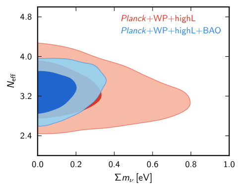
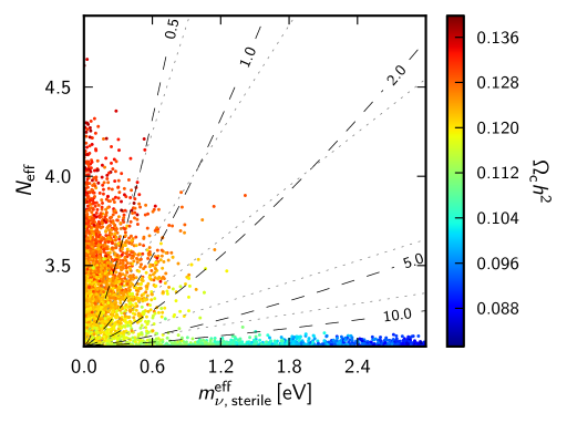
In the second model, we assume the existence of one massive sterile neutrino, in addition to the two massless and one massive active neutrino of the base model. The active neutrino mass is kept fixed at $0.06\thinspace\mathrm{eV}$. In particle physics, this assumption can be motivated in several ways. For example, there has recently been renewed interest in models with one light sterile neutrino in order to explain the MiniBoone anomaly reported in Aguilar-Arevalo et al. (2012), as well as reactor and Gallium anomalies (Giunti et al. 2013). The statistical significance of these results is marginal and they should not be over-interpreted. However, they do motivate investigating a model with three active neutrinos and one heavier sterile neutrino with mass $m_{\rm sterile}$. If the sterile neutrino were to thermalize with the same temperature as active neutrinos, this model would have $N_{\rm eff}\approx 4$.

Since we wish to be more general, we assume that the extra eigenstate is either: (i) thermally distributed with an arbitrary temperature $T_{\mathrm{s}}$; or (ii) distributed proportionally to active neutrinos with an arbitrary scaling factor $\chi_{\rm s}$ in which the scaling factor is a function of the active–sterile neutrino mixing angle. This second case corresponds the Dodelson-Widrow scenario (Dodelson & Widrow 1994). The two cases are in fact equivalent for cosmological observables and do not require separate analyses (Colombi et al. 1996; Lesgourgues et al. 2013). Sampling the posterior with flat priors on $N_{\rm eff}$ and $m_{\rm sterile}$ would not be efficient, since in the limit of small temperature $T_{\mathrm{s}}$, or small scaling factor $\chi_{\rm s}$, the mass would be unbounded. Hence we adopt a flat prior on the “effective sterile neutrino mass” defined as $m_{\nu,\thinspace\mathrm{sterile}}^{\mathrm{eff}}\equiv(94.1\omega_{\nu,\thinspace\mathrm{sterile}})\thinspace\mathrm{eV}$. In the case of a thermally-distributed sterile neutrino, this parameter is related to the true mass via

$$m_{\nu,\thinspace\mathrm{sterile}}^{\mathrm{eff}}=(T_{\mathrm{s}}/T_{\nu})^{3}m_{\rm sterile}^{\rm thermal}=(\Delta N_{\rm eff})^{3/4}m_{\rm sterile}^{\rm thermal}\thinspace.$$ (85)

Here, recall that $T_{\nu}=(4/11)^{1/3}T_{\gamma}$ is the active neutrino temperature in the instantaneous-decoupling limit and that the effective number is defined via the energy density, $\Delta N_{\rm eff}=(T_{\mathrm{s}}/T_{\nu})^{4}$. In the Dodelson-Widrow case the relation is given by

$$m_{\nu,\thinspace\mathrm{sterile}}^{\mathrm{eff}}=\chi_{\rm s}m_{\rm sterile}^{\rm DW}\thinspace,$$ (86)

with $\Delta N_{\rm eff}=\chi_{\rm s}$. For a thermalized sterile neutrino with temperature $T_{\nu}$ (i.e., the temperature the active neutrinos would have if there were no heating at electron-positron annihilation), corresponding to $\Delta N_{\rm eff}=1$, the three masses are equal to each other.

Assuming flat priors on $N_{\rm eff}$ and $m_{\nu,\thinspace\mathrm{sterile}}^{\mathrm{eff}}$ with $m_{\nu,\thinspace\mathrm{sterile}}^{\mathrm{eff}}<3\thinspace\mathrm{eV}$, we find the results shown in Fig. 28. The physical mass, $m_{\rm sterile}^{\rm thermal}$ in the thermal scenario is constant along the dashed lines in the figure and takes the indicated value in $\mathrm{eV}$. The physical mass, $m_{\rm sterile}^{\rm DW}$, in the Dodelson-Widrow scenario is constant on the dotted lines. For low $N_{\rm eff}$ the physical mass of the neutrinos becomes very large, so that they become non-relativistic well before recombination. In the limit in which the neutrinos become non-relativistic well before any relevant scales enter the horizon, they will behave exactly like cold dark matter, and hence are completely unconstrained within the overall total constraint on the dark matter density. For intermediate cases where the neutrinos become non-relativistic well before recombination they behave like warm dark matter. The approach to the massive limit gives the tail of allowed models with large $m_{\nu,\thinspace\mathrm{sterile}}^{\mathrm{eff}}$ and low $N_{\rm eff}$ shown in Fig. 28, with increasing $m_{\nu,\thinspace\mathrm{sterile}}^{\mathrm{eff}}$ being compensated by decreased $\Omega_{\mathrm{c}}h^{2}$ to maintain the total level required to give the correct shape to the CMB power spectrum.

For low $m_{\nu,\thinspace\mathrm{sterile}}^{\mathrm{eff}}$ and $\Delta N_{\rm eff}$ away from zero the physical neutrino mass is very light, and the constraint becomes similar to the massless case. The different limits are continuously connected, and given the complicated shape seen in Fig. 28 it is clearly not appropriate to quote fully marginalized parameter constraints that would depend strongly on the assumed upper limit on $m_{\nu,\thinspace\mathrm{sterile}}^{\mathrm{eff}}$. Instead we restrict attention to the case where the physical mass is $m_{\rm sterile}^{\rm thermal}<10\thinspace\mathrm{eV}$, which roughly defines the region where (for the CMB) the particles are distinct from cold or warm dark matter. Using the Planck+WP+highL (abbreviated to CMB below) data combination, this gives the marginalized one-parameter constraints

$$\left.\begin{array}[]{c}N_{\rm eff}<3.91\\ m_{\nu,\thinspace\mathrm{sterile}}^{\mathrm{eff}}<0.59\thinspace\mathrm{eV}\end{array}\right\}\quad\mbox{(95\%; CMB for $m_{\rm sterile}^{\rm thermal}<10\thinspace\mathrm{eV}$)}\thinspace.$$ (87)

Combining further with BAO these tighten to

$$\left.\begin{array}[]{c}N_{\rm eff}<3.80\\ m_{\nu,\thinspace\mathrm{sterile}}^{\mathrm{eff}}<0.42\thinspace\mathrm{eV}\end{array}\right\}\hskip 5.69054pt\mbox{(95\%; CMB+BAO for $m_{\rm sterile}^{\rm thermal}<10\thinspace\mathrm{eV}$)}\thinspace.$$ (90)

These bounds are only marginally compatible with a fully thermalized sterile neutrino ($N_{\rm eff}\approx 4$) with sub-eV mass $m_{\rm sterile}^{\rm thermal}\approx m_{\nu,\thinspace\mathrm{sterile}}^{\mathrm{eff}}<0.5\thinspace\mathrm{eV}$ that could explain the oscillation anomalies. The above contraints are also appropriate for the Dodelson-Widrow scenario, but for a physical mass cut of $m_{\rm sterile}^{\rm DW}<20\thinspace\mathrm{eV}$.

The thermal and Dodelson-Widrow scenarios considered here are representative of a large number of possible models that have recently been investigated in the literature (Hamann et al. 2011; Diamanti et al. 2012; Archidiacono et al. 2012; Hannestad et al. 2012).

6.4 Big bang nucleosynthesis

Observations of light elements abundances created during big bang nucleosynthesis (BBN) provided one of the earliest precision tests of cosmology and were critical in establishing the existence of a hot big bang. Up-to-date accounts of nucleosynthesis are given by Iocco et al. (2009) and Steigman (2012). In the standard BBN model, the abundance of light elements (parameterized by $Y_{\rm P}^{\rm BBN}\equiv 4n_{\mathrm{He}}/n_{\rm b}$ for helium-4 and $y_{\rm DP}^{\rm BBN}\equiv 10^{5}n_{\mathrm{\rm D}}/n_{\mathrm{\rm H}}$ for deuterium, where $n_{i}$ is the number density of species $i$) can be predicted as a function of the baryon density $\omega_{\rm b}$, the number of relativistic degrees of freedom parameterized by $N_{\mathrm{eff}}$, and of the lepton asymmetry in the electron neutrino sector. Throughout this subsection, we assume for simplicity that lepton asymmetry is too small to play a role at BBN. This is a reasonable assumption, since Planck data cannot improve existing constraints on the asymmetry. We also assume that there is no significant entropy increase between BBN and the present day, so that our CMB constraints on the baryon-to-photon ratio can be used to compute primordial abundances.

To calculate the dependence of $Y_{\rm P}^{\rm BBN}$ and $y_{\rm DP}^{\rm BBN}$ on the parameters $\omega_{\rm b}$ and $N_{\mathrm{eff}}$, we use the accurate public code PArthENoPE (Pisanti et al. 2008), which incorporates values of nuclear reaction rates, particle masses and fundamental constants, and an updated estimate of the neutron lifetime ($\tau_{\rm n}=880.1$ s; Beringer et al. 2012). Experimental uncertainties on each of these quantities lead to a theoretical error for $Y_{\rm P}^{\rm BBN}(\omega_{\rm b},N_{\mathrm{eff}})$ and $y_{\rm DP}^{\rm BBN}(\omega_{\rm b},N_{\mathrm{eff}})$. For helium, the error is dominated by the uncertainty in the neutron lifetime, leading to $\sigma(Y_{\rm P}^{\rm BBN})=0.0003$. For deuterium, the error is dominated by uncertainties in several nuclear rates, and is estimated to be $\sigma(y_{\rm DP}^{\rm BBN})=0.04$ (Serpico et al. 2004).

These predictions for the light elements can be confronted with measurements of their abundances, and also with CMB data (which is sensitive to $\omega_{\rm b}$, $N_{\mathrm{eff}}$, and $Y_{\rm P}$). We shall see below that for the base cosmological model with $N_{\mathrm{eff}}=3.046$ (or even for an extended scenario with free $N_{\mathrm{eff}}$) the CMB data predict the primordial abundances, under the assumption of standard BBN, with smaller uncertainties than those estimated for the measured abundances. Furthermore, the CMB predictions are consistent with direct abundance measurements.

6.4.1 Observational data on primordial abundances

The observational constraint on the primordial helium-4 fraction used in this paper is $Y_{\rm P}^{\rm BBN}=0.2534\pm 0.0083$ (68% CL) from the recent data compilation of Aver et al. (2012), based on spectroscopic observations of the chemical abundances in metal-poor H ii regions. The error on this measurement is dominated by systematic effects that will be difficult to resolve in the near future. It is reassuring that the independent and conservative method presented in Mangano & Serpico (2011) leads to an upper bound for $Y_{\rm P}^{\rm BBN}$ that is consistent with the above estimate. The recent measurement of the proto-Solar helium abundance by Serenelli & Basu (2010) provides an even more conservative upper bound, $Y_{\rm P}^{\rm BBN}<0.294$ at the $2\thinspace\sigma$ level.

For the primordial abundance of deuterium, data points show excess scatter above the statistical errors, indicative of systematic errors. The compilation presented in Iocco et al. (2009), based on data accumulated over several years, gives $y_{\rm DP}^{\rm BBN}=2.87\pm 0.22$ (68% CL). Pettini & Cooke (2012) report an accurate deuterium abundance measurement in the $z=3.04984$ low-metallicity damped Ly$\thinspace\alpha$ system in the spectrum of QSO SDSS J1419+0829, which they argue is particularly well suited to deuterium abundance measurements. These authors find $y_{\rm DP}^{\rm BBN}=2.535\pm 0.05$ (68% CL), a significantly tighter constraint than that from the Iocco et al. (2009) compilation. The Pettini-Cooke measurement is, however, a single data point, and it is important to acquire more observations of similar systems to assess whether their error estimate is consistent with possible sources of systematic error. We adopt a conservative position in this paper and compare both the Iocco et al. (2009) and the Pettini & Cooke (2012) measurements to the CMB predictions

We consider only the ⁴He and D abundances in this paper. We do not discuss measurements of ³He abundances since these provide only an upper bound on the true primordial ³He fraction. Likewise, we do not discuss lithium. There has been a long standing discrepancy between the low lithium abundances measured in metal-poor stars in our Galaxy and the predictions of BBN. At present it is not clear whether this discrepancy is caused by systematic errors in the abundance measurements, or has an “astrophysical” solution (e.g., destruction of primordial lithium) or is caused by new physics (see Fields 2011, for a recent review).

6.4.2 Planck predictions of primordial abundances in standard BBN

Figure 29: Predictions of standard BBN for the primordial abundance of ⁴He (top) and deuterium (bottom), as a function of the baryon density. The width of the green stripes corresponds to 68% uncertainties on nuclear reaction rates. The horizontal bands show observational bounds on primordial element abundances compiled by various authors, and the red vertical band shows the Planck+WP+highL bounds on $\omega_{\rm b}$ (all with 68% errors). BBN predictions and CMB results assume $N_{\mathrm{eff}}=3.046$ and no significant lepton asymmetry.

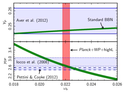
We first restrict ourselves to the base cosmological model, with no extra relativistic degrees of freedom beyond ordinary neutrinos (and a negligible lepton asymmetry), leading to $N_{\mathrm{eff}}=3.046$ (Mangano et al. 2005). Assuming that standard BBN holds, and that there is no entropy release after BBN, we can compute the spectrum of CMB anisotropies using the relation $Y_{\rm P}(\omega_{\rm b})$ given by PArthENoPE. This relation is used as the default in the grid of models discussed in this paper; we use the CosmoMC implementation developed by Hamann et al. (2008). The Planck+WP+highL  fits to the base $\Lambda$CDM  model gives the following estimate of the baryon density,

$$\omega_{\rm b}=0.02207\pm 0.00027\quad\mbox{(68\%; {Planck}+WP+highL)},$$ (92)

as listed in Table 5. In Fig. 29, we show this bound together with theoretical BBN predictions for $Y_{\rm P}^{\rm BBN}(\omega_{\rm b})$ and $y_{\rm DP}^{\rm BBN}(\omega_{\rm b})$. The bound of Eq. (92) leads to the predictions

$$Y_{\rm P}^{\rm BBN}(\omega_{\rm b}) = 0.24725\pm 0.00032,$$ (93a)

$$y_{\rm DP}^{\rm BBN}(\omega_{\rm b}) = 2.656\pm 0.067,$$ (93b)

where the errors here are 68% and include theoretical errors that are added in quadrature to those arising from uncertainties in $\omega_{\rm b}$. (The theoretical error dominates the total error in the case of $Y_{\rm P}$.) For helium, this prediction is in very good agreement with the data compilation of Aver et al. (2012), with an error that is 26 times smaller. For deuterium, the CMB+BBN prediction lies midway between the best-fit values of Iocco et al. (2009) and Pettini & Cooke (2012), but agrees with both at approximately the $1\thinspace\sigma$ level. These results strongly support standard BBN and show that within the framework of the base $\Lambda$CDM model, Planck  observations lead to extremely precise predictions of primordial abundances.

6.4.3 Estimating the helium abundance directly from Planck data

In the CMB analysis, instead of fixing $Y_{\rm P}$ to the BBN prediction, $Y_{\rm P}^{\rm BBN}(\omega_{\rm b})$, we can relax any BBN prior and let this parameter vary freely. The primordial helium fraction has an influence on the recombination history and affects CMB anisotropies mainly through the redshift of last scattering and the diffusion damping scale (Hu et al. 1995; Trotta & Hansen 2004; Ichikawa & Takahashi 2006; Hamann et al. 2008). Extending the base $\Lambda$CDM model by adding $Y_{\rm P}$ as a free parameter with a flat prior in the range $[0.1,0.5]$, we find

$$Y_{\rm P}=0.266\pm 0.021\quad\mbox{(68\%; {Planck}+WP+highL)}.$$ (94)

Constraints in the $Y_{\rm P}$–$\omega_{\mathrm{b}}$ plane are shown in Fig. 30. This figure shows that the CMB data have some sensitivity to the helium abundance. In fact, the error on the CMB estimate of $Y_{\rm P}$ is only $2.7$ times larger than the direct measurements of the primordial helium abundance by Aver et al. (2012). The CMB estimate of $Y_{\rm P}$ is consistent with the observational measurements adding further support in favour of standard BBN.

Figure 30: Constraints in the $\omega_{\mathrm{b}}$–$Y_{\rm P}$ plane from CMB and abundance measurements. The CMB constraints are for Planck+WP+highL (red 68% and 95% contours) in $\Lambda$CDM models with $Y_{\rm P}$ allowed to vary freely. The horizontal band shows observational bounds on ⁴He compiled by Aver et al. (2012) with 68% errors, while the grey region at the top of the figure delineates the conservative 95% upper bound inferred from Solar helium abundance by Serenelli & Basu (2010). The green stripe shows the predictions of standard BBN for the primordial abundance of ⁴He as a function of the baryon density (with 68% errors on nuclear reaction rates). Both BBN predictions and CMB results assume $N_{\mathrm{eff}}=3.046$ and no significant lepton asymmetry.

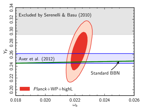
6.4.4 Extension to the case with extra relativistic relics

We now consider the effects of additional relativistic degrees of freedom on photons and ordinary neutrinos (obeying the standard model of neutrino decoupling) by adding $N_{\mathrm{eff}}$ as a free parameter. In the absence of lepton asymmetry, we can predict the BBN primordial abundances as a function of the two parameters $\omega_{\mathrm{b}}$ and $N_{\mathrm{eff}}$.

Figure 31: Constraints in the $\omega_{\mathrm{b}}$–$N_{\rm eff}$ plane from the CMB and abundance measurements. The blue stripes shows the 68% confidence regions from measurements of primordial element abundances assuming standard BBN: ⁴He bounds compiled by Aver et al. (2012); and deuterium bounds complied by Iocco et al. (2009) or measured by Pettini & Cooke (2012). We show for comparison the 68% and 95% contours inferred from Planck+WP+highL, when $N_{\mathrm{eff}}$ is left as a free parameter in the CMB analysis (and $Y_{\rm P}$ is fixed as a function of $\omega_{\rm b}$ and $N_{\mathrm{eff}}$ according to BBN predictions). These constraints assume no significant lepton asymmetry.

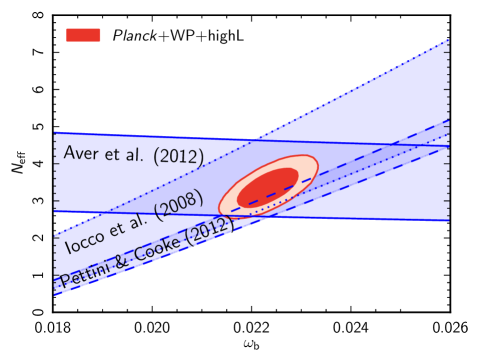
Figure 31 shows the regions in the $\omega_{\rm b}$–$N_{\mathrm{eff}}$ plane preferred by primordial abundance measurements, and by the CMB data if the standard BBN picture is correct. The regions allowed by the abundance measurements are defined by the $\chi^{2}$ statistic

$$\chi^{2}(\omega_{\rm b},N_{\mathrm{eff}})\equiv\frac{\left[y(\omega_{\rm b},N_{\mathrm{eff}})-y_{\mathrm{obs}}\right]^{2}}{\sigma_{\mathrm{obs}}^{2}+\sigma_{\mathrm{theory}}^{2}}\leavevmode\nobreak\ ,$$ (95)

where $y(\omega_{\rm b},N_{\mathrm{eff}})$ is the BBN prediction for either $Y^{\rm BBN}_{\rm P}$ or $y_{\rm DP}^{\rm BBN}$, the quantity $y_{\mathrm{obs}}$ is the observed abundance, and the two errors in the denominator are the observational and theoretical uncertainties. Figure 31 shows the edges of the 68% preferred regions in the $\omega_{\rm b}$–$N_{\mathrm{eff}}$ plane, given by $\chi^{2}=\chi^{2}_{\mathrm{min}}+2.3$.

For the CMB data, we fit a cosmological model with seven free parameters (the six parameters of the base $\Lambda$CDM model, plus $N_{\mathrm{eff}}$) to the Planck+WP+highL data, assuming that the primordial helium fraction is fixed by the standard BBN prediction $Y_{\rm P}^{\rm BBN}(\omega_{\rm b},N_{\mathrm{eff}})$. Figure 31 shows the joint 68% and 95% confidence contours in the $\omega_{\rm b}$–$N_{\mathrm{eff}}$ plane. The preferred regions in this plane from abundance measurements and the CMB agree remarkably well. The CMB gives approximately three times smaller error bars than primordial abundance data on both parameters.

We can derive constraints on $N_{\mathrm{eff}}$ from primordial element abundances and CMB data together by combining their likelihoods. The CMB-only confidence interval for $N_{\mathrm{eff}}$ is

$$N_{\mathrm{eff}}=3.36\pm 0.34\quad\mbox{(68\%; {Planck}+WP+highL)}.$$ (96)

When combined with the data reported respectively by Aver et al. (2012), Iocco et al. (2009), and Pettini & Cooke (2012), the 68% confidence interval becomes

$$N_{\mathrm{eff}}=\left\{\begin{tabular}[]{ll}$3.41\pm 0.30$,&$Y_{\rm P}$ (Aver et al.),\\ $3.43\pm 0.34$,&$y_{\rm DP}$ (Iocco et al.),\\ $3.02\pm 0.27$,&$y_{\rm DP}$ (Pettini and Cooke).\end{tabular}\right.$$ (97)

Since there is no significant tension between CMB and primordial element results, all these bounds are in agreement with the CMB-only analysis. The small error bar derived from combining the CMB with the Pettini & Cooke (2012) data point shows that further deuterium observations combined with Planck data have the potential to pin down the value of $N_{\mathrm{eff}}$ to high precision.

6.4.5 Simultaneous constraints on both $N_{\rm eff}$ and $Y_{\rm P}$

In this subsection, we discuss simultaneous constraints on both $N_{\rm eff}$ and $Y_{\rm P}$ by adding them to the six parameters of the base $\Lambda$CDM model. Both $N_{\rm eff}$ and $Y_{\rm P}$ have an impact on the damping tail of the CMB power spectrum by altering the ratio $k^{-1}_{\rm D}/r_{\ast}$, where $k^{-1}_{\rm D}$ is the photon diffusion length at last scattering and $r_{\ast}$ is the sound horizon there. There is thus an approximate degeneracy between these two parameters along which the ratio is nearly constant. The extent of the degeneracy is limited by the characteristic phase shift of the acoustic oscillations that arises due to the free streaming of the neutrinos (Bashinsky & Seljak 2004). As discussed by Hou et al. (2011), the early ISW effect also partly breaks the degeneracy, but this is less important than the effect of the phase shifts.

Figure 32: 2D joint posterior distribution for $N_{\rm eff}$ and $Y_{\rm P}$ with both parameters varying freely, determined from Planck+WP+highL data. Samples are colour-coded by the value of the angular ratio $\theta_{\rm D}/\theta_{\ast}$, which is constant along the degeneracy direction. The $N_{\rm eff}$–$Y_{\rm P}$ relation from BBN theory is shown by the dashed curve. The vertical line shows the standard value $N_{\rm eff}=3.046$. The region with $Y_{\rm P}>0.294$ is highlighted in grey, delineating the region that exceeds the $2\thinspace\sigma$ upper limit of the recent measurement of initial Solar helium abundance (Serenelli & Basu 2010), and the blue horizontal region is the 68% confidence region from the Aver et al. (2012) compilation of ⁴He measurements.

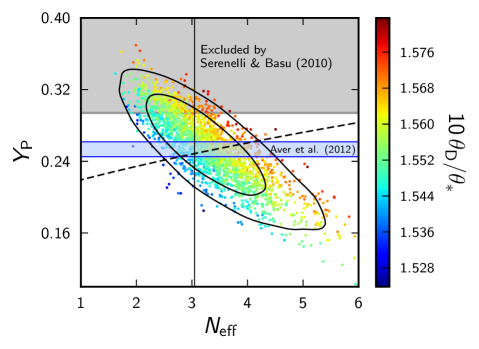
The joint posterior distribution for $N_{\rm eff}$ and $Y_{\rm P}$ from the Planck+WP+highL  likelihood is shown in Fig. 32, with each MCMC sample colour-coded by the value of the observationally-relevant angular ratio $\theta_{\rm D}/\theta_{\ast}\propto(k_{\rm D}r_{\ast})^{-1}$. The main constraint on $N_{\rm eff}$ and $Y_{\rm P}$ comes from the precise measurement of this ratio by the CMB, leaving the degeneracy along the constant $\theta_{\rm D}/\theta_{\ast}$ direction. The relation between $N_{\rm eff}$ and $Y_{\rm P}$ from BBN theory is shown in the figure by the dashed curve. The standard BBN prediction with $N_{\rm eff}=3.046$ is contained within the 68% confidence region. The grey region is for $Y_{\rm P}>0.294$ and is the $2\thinspace\sigma$ conservative upper bound on the primordial helium abundance from Serenelli & Basu (2010). Most of the samples are consistent with this bound. The inferred estimates of $N_{\rm eff}$ and $Y_{\rm P}$ from the Planck+WP+highL data are

$$N_{\rm eff} = 3.33_{-0.83}^{+0.59}\quad\hskip 0.56905pt\mbox{(68\%; {Planck}+WP+highL)},$$ (98a)

$$Y_{\rm P} = 0.254_{-0.033}^{+0.041}\quad\mbox{(68\%; {Planck}+WP+highL)}.$$ (98b)

Figure 33: 2D joint posterior distribution between $N_{\rm eff}$ and $\theta_{\ast}$ for $\Lambda$CDM models with variable $N_{\rm eff}$ (blue) and variable $N_{\rm eff}$ and $Y_{\rm P}$ (red). Both cases are for Planck+WP+highL  data.

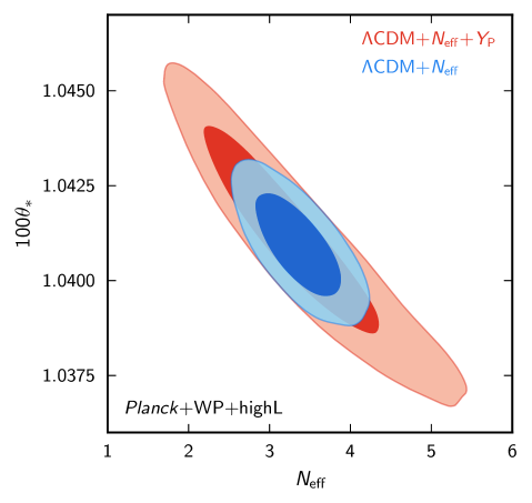
With $Y_{\rm P}$ allowed to vary, $N_{\rm eff}$ is no longer tightly constrained by the value of $\theta_{\rm D}/\theta_{\ast}$. Instead, it is constrained, at least in part, by the impact that varying $N_{\rm eff}$ has on the phase shifts of the acoustic oscillations. As discussed in Hou et al. (2012), this effect explains the observed correlation between $N_{\rm eff}$ and $\theta_{\ast}$, which is shown in Fig. 33. The correlation in the $\Lambda$CDM+$N_{\rm eff}$ model is also plotted in the figure showing that the $N_{\rm eff}$–$Y_{\rm P}$ degeneracy combines with the phase shifts to generate a larger dispersion in $\theta_{\ast}$ in such models.

6.5 Dark energy

A major challenge for cosmology is to elucidate the nature of the dark energy driving the accelerated expansion of the Universe. Perhaps the most straightforward explanation is that dark energy is a cosmological constant. An alternative is dynamical dark energy (Wetterich 1988; Ratra & Peebles 1988; Caldwell et al. 1998), usually based on a scalar field. In the simplest models, the field is very light, has a canonical kinetic energy term and is minimally coupled to gravity. In such models the dark energy sound speed equals the speed of light and it has zero anisotropic stress. It thus contributes very little to clustering. We shall only consider such models in this subsection.

A cosmological constant has an equation of state $w\equiv p/\rho=-1$, while scalar field models typically have time varying $w$ with $w\geq-1$. The analysis performed here is based on the “parameterized post-Friedmann” (PPF) framework of Hu & Sawicki (2007) and Hu (2008) as implemented in camb  (Fang et al. 2008b, a) and discussed earlier in Sect. 2. This allows us to investigate both regions of parameter space in which $w<-1$ (sometimes referred to as the “phantom” domain) and models in which $w$ changes with time.

Figure 34: Marginalized posterior distributions for the dark energy equation of state parameter $w$ (assumed constant), for Planck+WP alone (green) and in combination with SNe data (SNSL in blue and the Union2.1 compilation in red) or BAO data (black). A flat prior on $w$ from $-3$ to $-0.3$ was assumed and, importantly for the CMB-only constraints, the prior $[20,100]\thinspace{\rm km}\thinspace{\rm s}^{-1}\thinspace{\rm Mpc}^{-1}$ on $H_{0}$. The dashed grey line indicates the cosmological constant solution, $w=-1$.

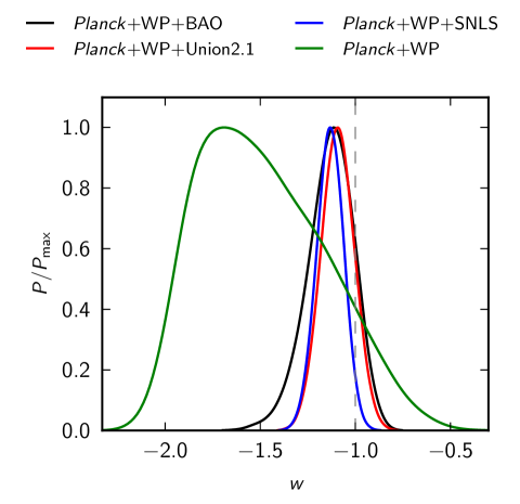
Figure 34 shows the marginalized posterior distributions for $w$ for an extension of the base $\Lambda$CDM cosmology to models with constant $w$. We present results for Planck+WP and in combination with SNe or BAO data. (Note that adding in the high-$\ell$ data from ACT and SPT results in little change to the posteriors shown in Fig. 34.) As expected, the CMB alone does not strongly constrain $w$, due to the two-dimensional geometric degeneracy in these models. We can break this degeneracy by combining the CMB data with lower redshift distance measures. Adding in BAO data tightens the constraints substantially, giving

$$w=-1.13^{+0.24}_{-0.25}\quad\mbox{(95\%; {Planck}+WP+BAO)},$$ (99)

in good agreement with a cosmological constant ($w=-1$). Using supernovae data leads to the constraints

$$w = -1.09\pm 0.17\quad\mbox{(95\%; {Planck}+WP+Union2.1)},$$ (100a)

$$w = -1.13^{+0.13}_{-0.14}\quad\quad\mbox{(95\%; {Planck}+WP+SNLS)},$$ (100b)

The combination with SNLS data favours the phantom domain ($w<-1$) at $2\thinspace\sigma$, while the Union2.1 compilation is more consistent with a cosmological constant.

If instead we combine Planck+WP with the Riess et al. (2011) measurement of $H_{0}$, we find

$$w=-1.24^{+0.18}_{-0.19}\quad\mbox{(95\%; {Planck}+WP+$H_{0}$)},$$ (101)

which is in tension with $w=-1$ at more than the $2\thinspace\sigma$ level.

The results in Eqs. (99–101) reflect the tensions between the supplementary data sets and the Planck base $\Lambda$CDM cosmology discussed in Sect. 5. The BAO data are in excellent agreement with the Planck base $\Lambda$CDM model, so there is no significant preference for $w\neq-1$ when combining BAO with Planck. In contrast, the addition of the $H_{0}$ measurement, or SNLS SNe data, to the CMB data favours models with exotic physics in the dark energy sector. These trends form a consistent theme throughout this section. The SNLS data favours a lower $\Omega_{\rm m}$ in the $\Lambda$CDM model than Planck, and hence larger dark energy density today. The tension can be relieved by making the dark energy fall away faster in the past than for a cosmological constant, i.e., $w<-1$.

The constant $w$ models are of limited physical interest. If $w\neq-1$ then it is likely to change with time. To investigate this we consider the simple linear relation in Eq. (4), $w(a)=w_{0}+w_{a}(1-a)$, which has often been used in the literature (Chevallier & Polarski 2001; Linder 2003). This parameterization approximately captures the low-redshift behaviour of light, slowly-rolling minimally-coupled scalar fields (as long as they do not contribute significantly to the total energy density at early times) and avoids the complexity of scanning a large number of possible potential shapes and initial conditions. The dynamical evolution of $w(a)$ can lead to distinctive imprints in the CMB (Caldwell et al. 1998) which would show up in the Planck data.

Figure 35: 2D marginalized posterior distribution for $w_{0}$ and $w_{a}$ for Planck+WP+BAO data. The contours are 68% and 95%, and the samples are colour-coded according to the value of $H_{0}$. Independent flat priors of $-3<w_{0}<-0.3$ and $-2<w_{a}<2$ are assumed. Dashed grey lines show the cosmological constant solution $w_{0}=-1$ and $w_{a}=0$.

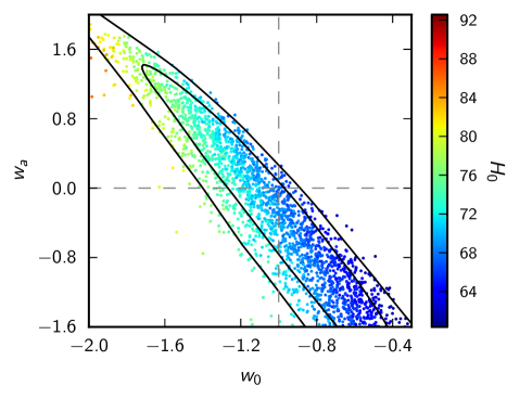
Figure 35 shows contours of the joint posterior distribution in the $w_{0}$–$w_{a}$ plane using Planck+WP+BAO data (colour-coded according to the value of $H_{0}$). The points are coloured by the value of $H_{0}$, which shows a clear variation with $w_{0}$ and $w_{a}$ revealing the three-dimensional nature of the geometric degeneracy in such models. The cosmological constant point $(w_{0},w_{a})=(-1,0)$ lies within the 68% contour and the marginalized posteriors for $w_{0}$ and $w_{a}$ are

$$w_{0} = -1.04^{+0.72}_{-0.69}\quad\mbox{(95\%; {Planck}+WP+BAO)},$$ (102a)

$$w_{a} < 1.32\hskip 34.1433pt\mbox{(95\%; {Planck}+WP+BAO)}.$$ (102b)

Including the $H_{0}$ measurement in place of the BAO data moves $(w_{0},w_{a})$ away from the cosmological constant solution towards negative $w_{a}$ at just under the $2\thinspace\sigma$ level.

Figure 36 shows likelihood contours for $(w_{0},w_{a})$, now adding SNe data to Planck. As discussed in detail in Sect. 5, there is a dependence of the base $\Lambda$CDM parameters on the choice of SNe data set, and this is reflected in Fig. 36. The results from the Planck+WP+Union2.1 data combination are in better agreement with a cosmological constant than those from the Planck+WP+SNLS combination. For the latter data combination, the cosmological constant solution lies on the $2\thinspace\sigma$ boundary of the $(w_{0},w_{a})$ distribution.

Figure 36: 2D marginalized posterior distributions for $w_{0}$ and $w_{a}$, for the data combinations Planck+WP+BAO (grey), Planck+WP+Union2.1 (red) and Planck+WP+SNLS (blue). The contours are 68% and 95%, and dashed grey lines show the cosmological constant solution.

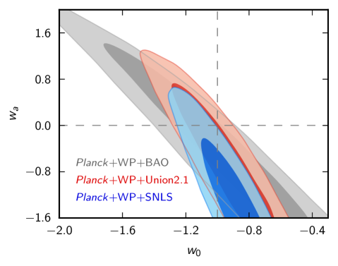
Dynamical dark energy models might also give a non-negligible contribution to the energy density of the Universe at early times. Such early dark energy (EDE; Wetterich 2004) models may be very close to $\Lambda$CDM recently, but have a non-zero dark energy density fraction, $\Omega_{\rm e}$, at early times. Such models complement the $(w_{0},w_{a})$ analysis by investigating how much dark energy can be present at high redshifts. EDE has two main effects: it reduces structure growth in the period after last scattering; and it changes the position and height of the peaks in the CMB spectrum.

The model we adopt here is that of Doran & Robbers (2006):

$$\Omega_{\rm de}(a)=\frac{\Omega_{\rm de}^{0}-\Omega_{\rm e}(1-a^{-3w_{0}})}{\Omega_{\rm de}^{0}+\Omega_{\rm m}^{0}a^{3w_{0}}}+\Omega_{\rm e}(1-a^{-3w_{0}})\thinspace\thinspace.$$ (103)

It requires two additional parameters to those of the base $\Lambda$CDM model: $\Omega_{\rm e}$, the dark energy density relative to the critical density at early times (assumed constant in this treatment); and the present-day dark energy equation of state parameter $w_{0}$. Here $\Omega_{\rm m}^{0}$ is the present matter density and $\Omega_{\rm de}^{0}=1-\Omega_{\rm m}^{0}$ is the present dark energy abundance (for a flat Universe). Note that the model of Eq. (103) has dark energy present over a large range of redshifts; the bounds on $\Omega_{\rm e}$ can be substantially weaker if dark energy is only present over a limited range of redshifts (Pettorino et al. 2013). The presence or absence of dark energy at the epoch of last scattering is the dominant effect on the CMB anisotropies and hence the constraints are insensitive to the addition of low redshift supplementary data such as BAO.

The most precise bounds on EDE arise from the analysis of CMB anisotropies (Doran et al. 2001; Caldwell et al. 2003; Calabrese et al. 2011; Reichardt et al. 2012; Sievers et al. 2013; Hou et al. 2012; Pettorino et al. 2013). Using Planck+WP+highL, we find

$$\Omega_{\rm e}<0.009\quad\mbox{(95\%; {Planck}+WP+highL)}.$$ (104)

(The limit for Planck+WP is very similar: $\Omega_{\rm e}<0.010$.) These bounds are consistent with and improve the recent ones of Hou et al. (2012), who give $\Omega_{e}<0.013$ at 95% CL, and Sievers et al. (2013), who find $\Omega_{e}<0.025$ at 95% CL.

In summary, the results on dynamical dark energy (except for those on early dark energy discussed above) are dependent on exactly what supplementary data are used in conjunction with the CMB data. (Planck lensing does not significantly improve the constraints on the models discussed here.) Using the direct measurement of $H_{0}$, or the SNLS SNe sample, together with Planck we see preferences for dynamical dark energy at about the $2\thinspace\sigma$ level reflecting the tensions between these data sets and Planck in the $\Lambda$CDM model. In contrast, the BAO measurements together with Planck give tight constraints which are consistent with a cosmological constant. Our inclination is to give greater weight to the BAO measurements and to conclude that there is no strong evidence that the dark energy is anything other than a cosmological constant.

6.6 Dark matter annihilation

Energy injection from dark matter (DM) annihilation can change the recombination history and affect the shape of the angular CMB spectra (Chen & Kamionkowski 2004; Padmanabhan & Finkbeiner 2005; Zhang et al. 2006; Mapelli et al. 2006). As recently shown in several papers (see e.g., Galli et al. 2009, 2011; Giesen et al. 2012; Hutsi et al. 2011; Natarajan 2012; Evoli et al. 2013) CMB anisotropies offer an opportunity to constrain DM annihilation models.

High-energy particles injected in the high-redshift thermal gas by DM annihilation are typically cooled down to the keV scale by high energy processes; once the shower has reached this energy scale, the secondary particles produced can ionize, excite or heat the thermal gas (Shull & van Steenberg 1985; Valdes et al. 2010); the first two processes modify the evolution of the free electron fraction $x_{\rm e}$, while the third affects the temperature of the baryons.

The rate of energy release, $dE/dt$, per unit volume by a relic annihilating DM particle is given by

$$\frac{dE}{dt}(z)=2\thinspace g\thinspace\rho^{2}_{\rm c}c^{2}\Omega^{2}_{\rm c}(1+z)^{6}p_{\rm ann}(z),\thinspace\thinspace\thinspace$$ (105)

where $p_{\rm ann}$ is, in principle, a function of redshift $z$, defined as

$$p_{\rm ann}(z)\equiv f(z)\frac{\langle\sigma v\rangle}{m_{\chi}},$$ (106)

where $\langle\sigma v\rangle$ is the thermally averaged annihilation cross-section, $m_{\chi}$ is the mass of the DM particle, $\rho_{\rm c}$ is the critical density of the Universe today, $g$ is a degeneracy factor equal to $1/2$ for Majorana particles and $1/4$ for Dirac particles (in the following, constraints will refer to Majorana particles), and the parameter $f(z)$ indicates the fraction of energy which is absorbed overall by the gas at redshift $z$.

In Eq. (106), the factor $f(z)$ depends on the details of the annihilation process, such as the mass of the DM particle and the annihilation channel (see e.g., Slatyer et al. 2009). The functional shape of $f(z)$ can be taken into account using generalized parameterizations (Finkbeiner et al. 2012; Hutsi et al. 2011). However, as shown in Galli et al. (2011), Giesen et al. (2012), and Finkbeiner et al. (2012) it is possible to neglect the redshift dependence of $f(z)$ to first approximation, since current data shows very little sensitivity to variations of this function. The effects of DM annihilation can therefore be well parameterized by a single constant parameter, $p_{\rm ann}$, that encodes the dependence on the properties of the DM particles.

We compute here the theoretical angular power in the presence of DM annihilations, by modifying the RECFAST routine in the camb code as in Galli et al. (2011) and by making use of the package CosmoMC for Monte Carlo parameter estimation. We checked that we obtain the same results by using the CLASS Boltzmann code (Lesgourgues 2011a) and the Monte Python package (Audren et al. 2012), with DM annihilation effects calculated either by RECFAST or HyRec (Ali-Haimoud & Hirata 2011), as detailed in Giesen et al. (2012). Besides $p_{\rm ann}$, we sample the parameters of the base $\Lambda$CDM model and the foreground/nuisance parameters described in Sect. 4.

From Planck+WP we find

$$p_{\rm ann}<5.4\times 10^{-6}\thinspace\mathrm{m}^{3}\thinspace\mathrm{s}^{-1}\thinspace\mathrm{kg}^{-1}\quad\mbox{(95; {Planck}+WP)}.$$ (107)

This constraint is weaker than that found from the full WMAP9 temperature and polarization likelihood, $p_{\rm ann}<1.2\times 10^{-6}\thinspace\mathrm{m^{3}s^{-1}kg^{-1}}$ because the Planck likelihood does not yet include polarization information at intermediate and high multipoles. In fact, the damping effect of DM annihilation on the CMB temperature power spectrum is highly degenerate with other cosmological parameters, in particular with the scalar spectral index and the scalar amplitude, as first shown by Padmanabhan & Finkbeiner (2005). As a consequence, the constraint on the scalar spectral index is significantly weakened when $p_{\rm ann}$ is allowed to vary, $n_{\rm s}=0.984^{+0.012}_{-0.026}$, to be compared to the constraint listed in Table 2 for the base $\Lambda$CDM cosmology, $n_{\rm s}=0.9603\pm 0.0073$.

These degeneracies can be broken by polarization data. The effect of DM annihilation on polarization is in fact an overall enhancement of the amplitude at large and intermediate scales, and a damping at small scales (see e.g., Fig. 1 in Galli et al. 2009 or Fig. 3 in Giesen et al. 2012). We thus expect the constraint to improve significantly with the forthcoming Planck polarization data release. We verified that adding BAO, HST or highL data to Planck+WP improves the constraints only marginally, as these datasets are not able to break the degeneracy between $p_{\rm ann}$ and $n_{\rm s}$.

On the other hand, we observe a substantial improvement in the constraints when we combine the Planck+WP data with the Planck lensing likelihood data. For this data combination we find an upper limit of

$$p_{\rm ann}<3.1\times 10^{-6}\thinspace\mathrm{m}^{3}\thinspace\mathrm{s}^{-1}\thinspace\mathrm{kg}^{-1}\quad\mbox{(95\%; {Planck}+lensing+WP}).$$ (108)

The improvement over Eq. (107) comes from the constraining power of the lensing likelihood on $A_{\rm s}$ and $n_{\rm s}$, that partially breaks the degeneracy with $p_{\rm ann}$.

Our results are consistent with previous work and show no evidence for DM annihilation. Future release of Planck polarization data will help to break the degeneracies which currently limit the accuracy of the constraints presented here.

6.7 Constraints on a stochastic background of primordial magnetic fields

Large-scale magnetic fields of the order of a few $\mu$G observed in galaxies and galaxy clusters may be the product of the amplification during structure formation, of primordial magnetic seeds (Ryu et al. 2012). Several models of the early Universe predict the generation of primordial magnetic fields (hereafter PMF), either during inflation or during later phase transitions (see Widrow 2002 and Widrow et al. 2012 for reviews).

PMF have an impact on cosmological perturbations and in particular on CMB anisotropy angular power spectra (Subramanian 2006), that can be used to constrain the PMF amplitude. In this section we will derive the constraints from Planck data on a stochastic background of PMF. We are mainly interested in constraints from CMB temperature anisotropies. Therefore, we will not consider the effect of Faraday rotation on CMB polarization anisotropies (Kosowsky & Loeb 1996; Kosowsky et al. 2005) nor non-Gaussianities associated with PMF (Brown & Crittenden 2005; Caprini et al. 2009; Seshadri & Subramanian 2009; Trivedi et al. 2010). We will restrict the analysis reported here to the non-helical case.

A stochastic background of PMF is modelled as a fully inhomogeneous component whose energy-momentum tensor is quadratic in the fields. We assume the usual magnetohydrodynamics limit, in which PMF are frozen and the time evolution is simply given by the dilution with cosmological expansion, $B(k,\eta)=B(k)/a(\eta)^{2}$. We model the PMF with a simple power-law power spectrum: $P_{B}(k)=Ak^{n_{B}}$, with a sharp cut off at the damping scale $k_{\rm D}$, as computed in Jedamzik et al. (1998) and Subramanian & Barrow (1998), to model the suppression of PMF on small scales.

It is customary to specify the amplitude of the PMF power spectrum with $B_{\lambda}$, the root-mean-square of the field smoothed over length scale $\lambda$, defined such that

$$B^{2}_{\lambda}=\int_{0}^{\infty}\frac{d{k\thinspace k^{2}}}{2\pi^{2}}e^{-k^{2}\lambda^{2}}P_{B}(k).$$ (109)

Given our assumed model and conventions, PMF are fully described by two parameters: the smoothed amplitude $B_{\lambda}$; and the spectral index $n_{B}$. Here, we set $\lambda=1\thinspace$Mpc and hence use $B_{1\thinspace\mathrm{Mpc}}$ as the parameter.

The components of the energy momentum tensor of PMF source all types of linear cosmological perturbations, i.e., scalar, vector, and tensor. In particular, the source terms are given by the magnetic energy density and anisotropic stress for scalar magnetized perturbations, whereas vector and tensor modes are sourced only by the magnetic anisotropic stress. In addition, both scalar and vector perturbations are affected by the Lorentz force; PMF induce a Lorentz force on baryons modifying their evolution and in particular their velocity, but during the tight-coupling regime between matter and radiation the Lorentz force also has an indirect effect on photons.

For the computation of magnetized angular power spectra, we use the analytic approximations for the PMF energy-momentum tensor components given in Paoletti & Finelli (2011). We consider here the regular mode for magnetic scalar perturbations, with the initial conditions of Paoletti et al. (2009) (see Giovannini 2004 for earlier calculations) and Shaw & Lewis (2010) (which describes the singular passive mode, depending on the generation time of PMF).

Previous analyses show that the main impact of PMF on the CMB anisotropy angular power spectrum is at small angular scales, well into the Silk damping regime. The dominant mode is the magnetic vector mode which peaks at $\ell\sim 2000$–3000 (Mack et al. 2002; Lewis 2004). The scalar magnetic mode is the dominant PMF contribution on large and intermediate angular scales (Giovannini 2007; Giovannini & Kunze 2008; Finelli et al. 2008). The tensor contribution is always subdominant with respect to the other two and it is negligible for the purposes of this analysis.

We include the scalar and vector magnetized contributions to the angular power spectrum within the MCMC analysis to derive the constraints on the PMF amplitude and spectral index using Planck $TT$ data. We vary the magnetic parameters $B_{1\thinspace\mathrm{Mpc}}/{\rm nG}$ and $n_{B}$, in addition to the other cosmological parameters of the base $\Lambda$CDM cosmology (this analysis assumes massless neutrinos, rather than the default value of a single eigenstate of mass $0.06\ {\rm eV}$ used in the rest of this paper). We adopt as prior ranges for the parameters $\left[0\thinspace,10\right]$ for $B_{1\thinspace\mathrm{Mpc}}/{\rm nG}$ and $\left[-2.99\thinspace,3\right]$ for the spectral index $n_{B}$. The lower bound $n_{B}>-3$ is necessary to avoid infrared divergences in the PMF energy momentum tensor correlators.

Figure 37: Constraints on the root-mean-square amplitude of the primordial magnetic field (for a smoothing scale of $1\thinspace{\rm Mpc}$) obtained with Planck+WP (black) and Planck+WP+highL (red).

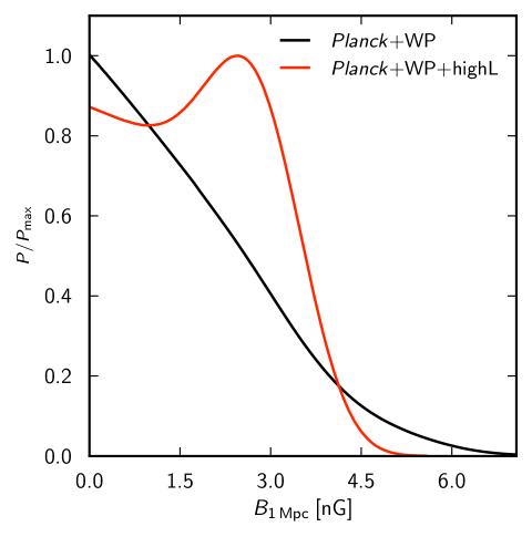
We perform analyses with Planck+WP and Planck+WP+highL likelihood combinations. Results are shown in Fig. 37. We find that the cosmological parameters are in agreement with those estimated assuming no PMF, confirming that the magnetic parameters are not degenerate with the cosmological parameters of the base $\Lambda$CDM model. The constraints on PMF with the Planck+WP likelihood are $B_{1\thinspace\mathrm{Mpc}}<4.1\thinspace$nG, with a preference for negative spectral indices at the $95\%$ confidence level. These limits are improved using Planck+WP+highL to $B_{1\thinspace\mathrm{Mpc}}<3.4\thinspace$nG with $n_{B}<0$ preferred at the $95\%$ confidence level. The new constraints are consistent with, and slightly tighter, than previous limits based on combining WMAP-7 data with high-resolution CMB data (see e.g. Paoletti & Finelli 2011; Shaw & Lewis 2012; Paoletti & Finelli 2012).

6.8 Constraints on variation of the fine-structure constant

Table 11: Constraints on the cosmological parameters of the base $\Lambda$CDM model with the addition of a varying fine-structure constant. We quote $\pm 1\thinspace\sigma$ errors. Note that for WMAP there is a strong degeneracy between $H_{0}$ and $\alpha$, which is why the error on $\alpha/\alpha_{0}$ is much larger than for Planck.

Planck+WP Planck+WP+BAO WMAP-9 $$\Omega_{\rm b}h^{2} 0.02206\pm 0.00028 0.02220\pm 0.00025 0.02309\pm 0.00130 \Omega_{\rm c}h^{2} 0.1174\pm 0.0030 0.1161\pm 0.0028 0.1148\pm 0.0048 \tau 0.095\pm 0.014 0.097\pm 0.014 0.089\pm 0.014 H_{0} 65.2\pm 1.8\kern 4.00002pt 66.7\pm 1.1\kern 4.00002pt 74\pm 11 n_{\rm s} 0.974\pm 0.012 0.975\pm 0.012 0.973\pm 0.014 \log(10^{10}A_{\rm s}) 3.106\pm 0.029 3.100\pm 0.029 3.090\pm 0.039 \alpha/\alpha_{0} 0.9936\pm 0.0043 0.9989\pm 0.0037 1.008\pm 0.020$$. . . . . . .

Figure 38: Left: Likelihood contours (68% and 95%) in the $\alpha/\alpha_{0}$–$H_{0}$ plane for the WMAP-9 (red), Planck+WP (blue), Planck+WP+$H_{0}$ (purple), and Planck+WP+BAO (green) data combinations. Middle: As left, but in the $\alpha/\alpha_{0}$–$\Omega_{\rm b}h^{2}$ plane. Right: Marginalized posterior distributions of $\alpha/\alpha_{0}$ for these data combinations.

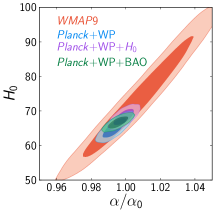
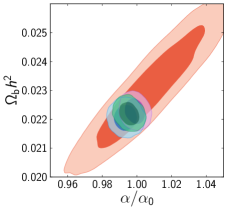
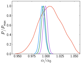
The $\Lambda$CDM model assumes the validity of General Relativity on cosmological scales, as well as the physics of the standard model of particle physics. One possible extension, which may have motivations in fundamental physics, is to consider variations of dimensionless constants. Such variations can be constrained through tests on astrophysical scales (Uzan 2003, 2011).

A number of physical systems have been used, spanning different time scales, to set constraints on variations of the fundamental constants. These range from atomic clocks in the laboratory at a redshift $z=0$ to BBN at $z\sim 10^{8}$. However, apart from the claims of varying $\alpha$ based on high resolution quasar absorption-line spectra  (Webb et al. 2001; Murphy et al. 2003), there is no other evidence for time-variable fundamental constants.

CMB temperature anisotropies have been used extensively to constrain the variation of fundamental constants over cosmic timescales. The temperature power spectrum is sensitive to the variation of the fine-structure constant $\alpha$, the electron-to-proton mass ratio $\mu$, and the gravitational constant $\alpha_{\rm g}\equiv Gm_{\rm p}^{2}/\hbar c$. A variation of $G$ can affect the Friedmann equation, and also raises the issue of consistency in the overall theory of gravity. However, a variation of the non-gravitational constants ($\alpha$ and $m_{\rm e}$) is more straightforward to analyse, mostly inducing a modification of the interaction between light and atoms (shifts in the energy levels and binding energy of hydrogen and helium). This induces a modification of the ionization history of the Universe. In particular, a variation of $\alpha$ modifies the redshift of recombination through the shift in the energy levels and the Thomson scattering cross-section. An increase in $\alpha$ induces a shift of the position of the first acoustic peak, which is inversely proportional to the sound horizon at last scattering. The larger redshift of last scattering also produces a larger early ISW effect, and hence a higher amplitude of the first acoustic peak. Finally, an increase in $\alpha$ decreases diffusive damping at high multipoles. For earlier studies of varying constants using the CMB (see e.g., Kaplinghat et al. 1999; Avelino et al. 2000; Martins et al. 2004; Rocha et al. 2004; Nakashima et al. 2008, 2010; Menegoni et al. 2009; Landau & Scóccola 2010).

The analysis presented here focuses solely on the time variation of the fine-structure constant $\alpha$, in addition to the parameters of the base $\Lambda$CDM model, using a modified form of the RECFAST recombination code (Hannestad 1999; Martins et al. 2004; Rocha et al. 2004). Selected results are given in Table 11, which compares parameter constraints from Planck and from our own analysis of the full WMAP-9 $TT$, $TE$ and $EE$ likelihood. From CMB data alone, Planck improves the constraints from a $2\%$ variation in $\alpha$ to about $0.4\%$. Planck thus improves the limit by a factor of around five, while the constraints on the parameters of the base $\Lambda$CDM model change very little with the addition of a time-varying $\alpha$. These results are in good agreement with earlier forecasts (Rocha et al. 2004).

Given the apparent tension between the base $\Lambda$CDM parameters from Planck and direct measurements of $H_{0}$ discussed in Sect. 5.3), we include further information from the $H_{0}$ prior  and BAO data (see Sect. 5.2). Figure 38 compares the constraints in the ($\alpha/\alpha_{0},H_{0}$) and ($\alpha/\alpha_{0},\Omega_{\rm b}h^{2}$) planes and also shows the marginalized posterior distribution of $\alpha/\alpha_{0}$ for the various data combinations.

The constraint on $\alpha$ is slightly improved by including the BAO data (via a tightening of the parameters of the base $\Lambda$CDM model). Note that the central value of the prior on $H_{0}$ is outside the 95% confidence region, even for the Planck+WP+$H_{0}$ combination. Adding a varying $\alpha$ does not resolve the tension between direct measurements of $H_{0}$ and the value determined from the CMB.

In summary, Planck data improve the constraints on $\alpha/\alpha_{0}$, with respect to those from WMAP-9 by a factor of about five. Our analysis of Planck data limits any variation in the fine-structure constant from $z\sim 10^{3}$ to the present day to be less than approximately $0.4\%$.

7 Discussion and conclusions

The most important conclusion from this paper is the excellent agreement between the Planck temperature power spectrum at high multipoles with the predictions of the base $\Lambda$CDM model. The base $\Lambda$CDM model also provides a good match to the Planck power spectrum of the lensing potential, $C^{\phi\phi}_{\ell}$, and to the $TE$ and $EE$ power spectra at high multipoles.

The high statistical significance of the Planck detection of gravitational lensing of the CMB leads to some interesting science conclusions using Planck data alone. For example, gravitational lensing breaks the “geometrical degeneracy” and we find that the geometry of the Universe is consistent with spatial flatness to percent-level precision using CMB data alone. The Planck lensing power spectrum also leads to an interesting constraint on the reionization optical depth of $\tau=0.089\pm 0.032$, independent of CMB polarization measurements at low multipoles.

The parameters of the base $\Lambda$CDM model are determined to extremely high precision by the Planck data. For example, the scalar spectral index is determined as $n_{\rm s}=0.9585\pm 0.0070$, a $6\thinspace\sigma$ deviation from exact scale invariance. Even in the base $\Lambda$CDM model, we find quite large changes in some parameters compared to previous CMB experiments. In particular, from Planck we find a low value of the Hubble constant, $H_{0}=(67.3\pm 1.2)\thinspace{\rm km}\thinspace{\rm s}^{-1}\thinspace{\rm Mpc}^{-1}$, and a high matter density, $\Omega_{\rm m}=0.315\pm 0.016$. If we accept that the base $\Lambda$CDM model is the correct cosmology, then as discussed in Sect. 5 Planck is in tension with direct measurements of the Hubble constant (at about the $2.5\thinspace\sigma$ level) and in mild tension with the SNLS Type Ia supernova compilation (at about the $2\thinspace\sigma$ level). For the base $\Lambda$CDM model, we also find a high amplitude for the present-day matter fluctuations, $\sigma_{8}=0.828\pm 0.012$, in agreement with previous CMB experiments. This value is higher than that inferred from counts of rich clusters of galaxies, including our own analysis of Planck cluster counts (Planck Collaboration XX 2014), and in tension with the cosmic shear measurements discussed in Sect. 5.5.2.

One possible interpretation of these tensions is that systematic errors are not completely understood in some astrophysical measurements. The fact that the Planck results for the base $\Lambda$CDM model are in such good agreement with BAO data, which are based on a simple geometrical measurement, lends support to this view. An alternative explanation is that the base $\Lambda$CDM model is incorrect. In summary, at high multipoles, the base $\Lambda$CDM cosmology provides an excellent fit to the spectra from Planck, ACT and SPT (for all frequency combinations), as illustrated in Figs. 7, 8 and 9, but the parameters derived from the CMB apparently conflict with some types of astrophysical measurement.

Figure 39: Left: Planck $TT$ spectrum at low multipoles with $68\%$ ranges on the posteriors. The “rainbow” band show the best fits to the entire Planck+WP+highL likelihood for the base $\Lambda$CDM cosmology, colour-coded according to the value of the scalar spectral index $n_{\rm s}$. Right: Limits (68% and 95%) on the relative amplitude of the base $\Lambda$CDM fits to the Planck+WP likelihood fitted only to the Planck $TT$ likelihood over the multipole range $2\leq\ell\leq\ell_{\rm max}$.

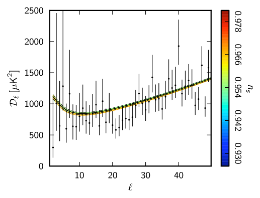
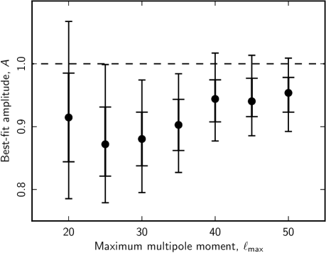
Before summarizing our results on extensions to the base $\Lambda$CDM model, it is worth making some remarks on foreground modelling and the impact of this modelling on our error estimates. The addition of CMB data at high multipoles helps to constrain the model of unresolved foregrounds, in particular, the contribution from “minor” components, such as the kinetic SZ, which are poorly constrained from Planck alone. For the base $\Lambda$CDM model, the cosmological parameters are not limited by foreground modelling, as illustrated in Fig. 4. As discussed in Appendix C, foreground modelling becomes more important in analysing extended CDM models, particularly those that have strong parameter degeneracies that are broken only via precision measurements of the damping tail in the CMB spectrum. As a crude measure of the importance of foreground modelling, we can compare parameter values with and without inclusion of the ACT and SPT data at high multipoles. A large shift in parameter values indicates a possible sensitivity to foreground modelling, and so any such result should be treated with caution. We have thus normally adopted the Planck+WP+highL likelihood combination as offering the most reliable results for extensions to the base $\Lambda$CDM cosmology.

From an analysis of an extensive grid of models, we find no strong evidence to favour any extension to the base $\Lambda$CDM cosmology, either from the CMB temperature power spectrum alone, or in combination with the Planck lensing power spectrum and other astrophysical data sets.

We find the following notable results using CMB data alone:

• The deviation of the scalar spectral index from unity is robust to the addition of tensor modes and to changes in the matter content of the Universe. For example, adding a tensor component we find $n_{\rm s}=0.9600\pm 0.0072$, a $5.5\thinspace\sigma$ departure from $n_{\rm s}=1$.

• A 95% upper limit on the tensor-to-scalar ratio of $r_{0.002}<0.11$. The combined contraints on $n_{\rm s}$ and $r_{0.002}$ are on the borderline of compatibility with single-field inflation with a quadratic potential (Fig. 23).

• A 95% upper limit on the summed neutrino mass of $\sum m_{\nu}<0.66\thinspace{\rm eV}$.

• A determination of the effective number of neutrino-like relativistic degrees of freedom of $N_{\rm eff}=3.36\pm 0.34$, compatible with the standard value of $3.046$.

• The results from Planck are consistent with the results of standard big bang nucleosynthesis. In fact, combining the CMB data with the most recent results on the deuterium abundance, leads to the constraint $N_{\rm eff}=3.02\pm 0.27$, again compatible with the standard value of $3.046$.

• New limits on a possible variation of the fine-structure constant, dark matter annihilation and primordial magnetic fields.

We also find a number of marginal (around $2\thinspace\sigma$) results, perhaps indicative of internal tension within the Planck data. Examples include the preference of the (phenomenological) lensing parameter for values greater than unity ($A_{\rm L}=1.23\pm 0.11$; Eq. 49) and for negative running ($dn_{\rm s}/d\ln k=-0.015\pm 0.09$; Eq. 67b). In Planck Collaboration XXII (2014), the Planck data indicate a preference for anti-correlated isocurvature modes and for models with a truncated power spectrum on large scales. None of these results have a decisive level of statistical significance, but they can all be traced to an unusual aspect of the temperature power spectrum at low multipoles. As can be seen in Fig. 1, and on an expanded scale in the left-hand panel of Fig. 39, the measured power spectrum shows a dip relative to the best-fit base $\Lambda$CDM cosmology in the multipole range $20\la\ell\la 30$ and an excess at $\ell=40$. The existence of “glitches” in the power spectrum at low multipoles was noted by the WMAP team in the first-year papers (Hinshaw et al. 2003; Spergel et al. 2003) and acted as motivation to fit an inflation model with a step-like feature in the potential (Peiris et al. 2003). Similar investigations have been carried out by a number of authors, (see e.g., Mortonson et al. 2009, and references therein). At these low multipoles, the Planck spectrum is in excellent agreement with the WMAP nine-year spectrum (Planck Collaboration XV 2014), so it is unlikely that any of the features such as the low quadrupole or “dip” in the multipole range $20$–$30$ are caused by instrumental effects or Galactic foregrounds. These are real features of the CMB anisotropies.

The Planck data, however, constrain the parameters of the base $\Lambda$CDM model to such high precision that there is little remaining flexibility to fit the low-multipole part of the spectrum. To illustrate this point, the right-hand panel of Fig. 39 shows the 68% and 95% limits on the relative amplitude of the base $\Lambda$CDM model (sampling the chains constrained by the full likelihood) fitted only to the Planck $TT$ likelihood over the multipole range $2\leq\ell\leq\ell_{\rm max}$. From multipoles $\ell_{\rm max}\approx 25$ to multipoles $\ell_{\rm max}\approx 35$, we see more than a $2\thinspace\sigma$ departure from values of unity. (The maximum deviation from unity is $2.7\thinspace\sigma$ at $\ell=30$.) It is difficult to know what to make of this result, and we present it here as a “curiosity” that needs further investigation. The Planck temperature data are remarkably consistent with the predictions of the base $\Lambda$CDM model at high multipoles, but it is also conceivable that the $\Lambda$CDM cosmology fails at low multipoles. There are other indications, from both WMAP and Planck data for “anomalies” at low multipoles (Planck Collaboration XXIII 2014), that may be indicative of new physics operating on the largest scales in our Universe. Interpretation of large-scale anomalies (including the results shown in Fig. 39) is difficult in the absence of a theoretical framework. The problem here is assessing the role of a posteriori choices, i.e., that inconsistencies attract our attention and influence our choice of statistical test. Nevertheless, we know so little about the physics of the early Universe that we should be open to the possibility that there is new physics beyond that assumed in the base $\Lambda$CDM model. Irrespective of the interpretation, the unusual shape of the low multipole spectrum is at least partly responsible for some of the $2\thinspace\sigma$ effects seen in the analysis of extensions to the $\Lambda$CDM model discussed in Sect. 6.

Supplementary information from astrophysical data sets has played an important role in the analysis of all previous CMB experiments. For Planck the interpretation of results combined with non-CMB data sets is not straightforward (as a consequence of the tensions discussed in Sect. 5). For the base $\Lambda$CDM model, the statistical power of the Planck data is so high that we find very similar cosmological parameters if we add the Riess et al. (2011) constraint on $H_{0}$, or either of the two SNe samples, to those derived from the CMB data alone. In these cases, the solutions simply reflect the tensions discussed in Sect. 5, for example, including the $H_{0}$ measurement with the Planck+WP likelihood we find $H_{0}=(68.6\pm 1.2)\thinspace{\rm km}\thinspace{\rm s}^{-1}\thinspace{\rm Mpc}^{-1}$, discrepant with the direct measurement at the $2.2\thinspace\sigma$ level.

The interpretation becomes more complex for extended models where astrophysical data is required to constrain parameters that cannot be determined accurately from CMB measurements alone. As an example, it is well known that CMB data alone provide weak constraints on the dark energy equation of state parameter $w$ (see Fig. 34). The addition of BAO data to the CMB data gives a tight constraint of $w=-1.13\pm 0.12$. However, adding the SNLS SNe data gives $w=-1.135\pm 0.069$ and adding the $H_{0}$ measurement gives $w=-1.244\pm 0.095$. Adding either of the two data sets which show tension with the CMB measurements for the base $\Lambda$CDM model, draws the solutions into the phantom domain ($w<-1$) at about the $2\thinspace\sigma$ level. In contrast, if we use the BAO data in addition to the CMB, we find no evidence for dynamical dark energy; these data are compatible with a cosmological constant, as assumed in the base $\Lambda$CDM model.

The impact of additional astrophysical data is particularly complex in our investigation of neutrino physics (Sect. 6.3). We will use the effective number of relativistic degrees of freedom, $N_{\rm eff}$ as an illustration. From the CMB data alone, we find $N_{\rm eff}=3.36\pm 0.34$. Adding BAO data gives $N_{\rm eff}=3.30\pm 0.27$. Both of these values are consistent with the standard value of $3.046$. Adding the $H_{0}$ measurement to the CMB data gives $N_{\rm eff}=3.62\pm 0.25$ and relieves the tension between the CMB data and $H_{0}$ at the expense of new neutrino-like physics (at around the $2.3\thinspace\sigma$ level). It is possible to alleviate the tensions between the CMB, BAO, $H_{0}$ and SNLS data by invoking new physics such as an increase in $N_{\rm eff}$. However, none of these cases are favoured significantly over the base $\Lambda$CDM model by the Planck data (and they are often disfavoured). Any preference for new physics comes almost entirely from the astrophysical data sets. It is up to the reader to decide how to interpret such results, but it is simplistic to assume that all astrophysical data sets have accurately quantified estimates of systematic errors. We have therefore tended to place greater weight on the CMB and BAO measurements in this paper rather than on more complex astrophysical data.

Our overall conclusion is that the Planck data are remarkably consistent with the predictions of the base $\Lambda$CDM cosmology. However, the mismatch with the temperature spectrum at low multipoles, evident in Figs. 1 and 39, and the existence of other “anomalies” at low multipoles, is possibly indicative that the model is incomplete. The results presented here are based on a first, and relatively conservative, analysis of the Planck data. The 2014 data release will use data obtained over the full mission lifetime of Planck, including polarization data. It remains to be seen whether these data, together with new astrophysical data sets and CMB polarization measurements, will offer any convincing evidence for new physics.

Appendix A Comparison of the Planck  and WMAP-9 base $\Lambda$CDM cosmologies

The parameters for the base $\Lambda$CDM cosmology derived from Planck differ from those derived from WMAP-9. In this appendix, we address the question of whether the parameter shifts are consistent statistically with the shifts expected from the additional multipole coverage of Planck.

We begin with a direct comparison of the shapes of the Planck and WMAP-9 spectra. Figure 40 shows our estimate of the combined V+W-band WMAP-9 power spectrum computed on the same mask used for the $100\times 100\thinspace{\rm GHz}$ Planck spectrum in the main text. Here we use a combined WMAP+Planck mask for point sources. The magenta points show the Planck $100\times 100$ GHz spectrum corrected for extra-Galactic foregrounds with the best-fit Planck+WP+highL parameters from Table 5. The WMAP points have been rescaled by a multiplicative factor of $0.974$ and agree to high precision point-by-point with the Planck spectrum. (Note that the errors plotted for the WMAP points show the noise errors and the cross-term between signal and noise computed from Monte Carlo simulations; they do not include CMB-foreground cross-correlations and correlated beam errors.) The rms scatter between the Planck and WMAP points over the multipole range $50\leq\ell\leq 400$ is only $16\thinspace\mu{\rm K}^{2}$, i.e., after a multiplicative scaling the two spectra are consistent to within about 0.5% of the primary CMB spectrum. Similar tests are described in greater detail in Planck Collaboration XXXI (2014), including comparisons with the LFI $70$ GHz spectrum. The reason for the multiplicative factor (amounting to a 1.3% difference in the calibrations of the HFI and WMAP maps) is not fully understood and is the subject of ongoing investigations. For the purposes of this appendix, we treat the rescaling as an empirical result, i.e., after accounting for a multiplicative calibration factor, the Planck and WMAP-9 power spectra agree to high precision, with little evidence for any significant variation of the spectra with multipole.

Figure 40: Comparison of the Planck and WMAP-9 power spectra. The green points show the combined WMAP-9 V+W-band spectrum computed on the same mask used for the $100\times 100$ GHz Planck spectrum (with a combined WMAP+Planck mask for point sources) after rescaling the WMAP power spectrum by a multiplicative factor of $0.974$. The magenta points show the Planck $100\times 100$ GHz spectrum computed on the same mask. The red line shows the best-fit Planck+WP+highL base $\Lambda$CDM model. The lower panel shows the residuals with respect to this model. The error bars on the WMAP points show the instrumental noise together with the noise-signal errors as discussed in the text; errors are not shown for Planck.

Table 12: Comparison of base $\rm{\Lambda CDM}$ parameters from WMAP-9 with Planck. The second column gives parameters derived from the WMAP-9 likelihood. The third column gives results for Planck+WP, with the Planck likelihood restricted to multipoles $\ell\leq 1000$. The fourth and fifth columns show results for the full Planck+WP and WMAP-9 likelihoods combined with the BAO data discussed in Sect. 5.2. As in the main body of the paper, we have assumed a neutrino mass of $0.06\;{\rm eV}$.

WMAP-9 Planck $$l\leq 1000$$+WP Planck+WP+BAO WMAP-9+BAO

Parameter 68% limits 68% limits 68% limits 68% limits

.

.

.

.

.

.

.

.

.

.

.

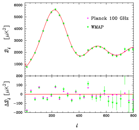
Given the agreement between the WMAP-9 and Planck spectra shown in Fig. 40, we should expect the two experiments to give similar cosmological parameters if the multipole range of Planck is restricted to $\ell\la 1000$. This is illustrated by the results of Table 12, which lists base $\rm{\Lambda CDM}$ parameters for WMAP-9 and for the Planck+WP likelihood limited to a maximum multipole of $\ell_{\rm max}=1000$. (For this restricted multipole range, we keep the foreground and other nuisance parameters fixed to the best-fit values derived from the full Planck+WP likelihood.) The cosmological parameters derived from these two likelihoods are in very good agreement. (See also Planck Collaboration XV (2014) and Appendix C for further tests of the variations of cosmological parameters from Planck as $\ell_{\rm max}$ is varied.)

Figure 41: Variations in $H_{0}$ and $n_{\rm s}$ as the maximum multipole in the Planck likelihood is increased from $\ell_{\rm max}=1000$ to $2500$. The red points show the changes in parameters determined from 2000 simulations, as described in the text. The blue point shows the changes determined from the real data.

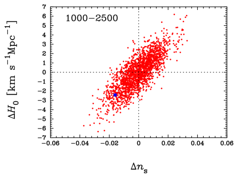
We should expect the best-fit cosmological parameters to change as the maximum multipole $\ell_{\rm max}$ is increased, since there is additional cosmological information at higher multipoles. As a useful rule-of-thumb, the covariance of the shifts in the best-fit parameters on adding further independent data should be approximately equal to the difference in the parameter covariances. To assess more carefully whether the cosmological parameter shifts seen in the Planck analysis of $\Lambda$CDM models are statistically reasonable, we perform a set of Fisher-matrix-type simulations. We draw Gaussian realizations of simulated spectra, $C^{\rm sim}_{\ell}$, from the frequency-compressed covariance matrix $\hat{\mathcal{M}}_{\ell\ell^{\prime}}$, introduced in Eq. (37), which includes contributions from beam and foreground errors. We adopt the best-fitting base $\rm{\Lambda CDM}$  model to the Planck+WP+highL data as our fiducial model $C^{\rm fid}_{\ell}$ and form

$$\chi^{2}=\sum_{\ell\ell^{\prime}}\Delta C_{\ell}\hat{\mathcal{M}}^{-1}_{\ell\ell^{\prime}}\Delta C_{\ell^{\prime}}+{(\Delta\tau)^{2}\over\sigma^{2}_{\tau}},$$ (110)

where

$$\Delta C_{\ell}=C^{\rm sim}_{\ell}-C^{\rm fid}_{\ell}-\sum_{p}{\partial C^{\rm fid}_{\ell}\over\partial a_{p}}\Delta a_{p},$$ (111)

and the $a_{p}$ are the cosmological parameters of the base model (taken here to be $A_{\rm s}$, $\omega_{\mathrm{b}}$, $\omega_{\mathrm{c}}$, $H_{0}$, $n_{\rm s}$ and $\tau$). Since these simulations are based only on the high multipole Planck likelihood, we include a prior on $\tau$ in Eq. (110) with $\sigma_{\tau}=0.014$. In addition, since the covariance matrix $\hat{{\cal M}}_{\ell\ell^{\prime}}$ includes estimates of foreground and beam errors, which are highly correlated over a wide multipole range, we add a “point source” amplitude as a catch-all to model uncertainties from nuisance parameters. With this machinery, we can quickly calculate the parameter shifts $\Delta a_{p}$ that minimise the $\chi^{2}$ in Eq. (110) for different choices of $\ell_{\rm max}$. (Note that these simulations reproduce to high precision the parameter errors and degeneracy directions of the full Planck likelihood.)

Results for $2000$ simulations are shown in Fig. 41 in the $H_{0}$–$n_{\rm s}$ plane. (The results are similar for the $\omega_{b}$–$\omega_{c}$ plane.) Each red point in Fig. 41 shows the parameter shifts measured from a single simulation as $\ell_{\rm max}$ is increased from 1000 to 2500. The blue point shows the shift in parameters for the real data. The shifts seen in the real data follow the degeneracy directions defined by the simulations (in all parameters) and lie within $1.6\thinspace\sigma$ of the dispersion of the simulated parameter shifts for any single parameter. We therefore conclude that the parameter shifts seen between Planck and WMAP-9 are statistically consistent with our expectations based on the further information contained in the power spectrum at high multipoles.

The last two columns in Table 12 list the base $\rm{\Lambda CDM}$ parameters for Planck+WP+BAO and for WMAP-9+BAO. Adding the baryon acoustic oscillation data to WMAP-9 brings the cosmological parameters closer to the Planck parameters (with or without the addition of the BAO data). This is what we would expect if the Planck base $\rm{\Lambda CDM}$ cosmology is correct and the Planck, WMAP-9 and BAO data are largely free of systematic errors.

Appendix B Comparison of the Planck  and SPT S12 base $\Lambda$CDM cosmologies

Figure 42: The acoustic scale distance ratio $r_{\rm s}/D_{V}(z)$ divided by the distance ratio of the best fit WMAP-7+SPT base $\rm{\Lambda CDM}$ cosmology of S12. The points are colour coded as follows: green star (6dF); purple squares (SDSS DR7 as analysed by Percival et al. 2010); black star (SDSS DR7 as analysed by Padmanabhan et al. 2012); blue cross (BOSS DR9); and blue circles (WiggleZ). Error bars show $1\thinspace\sigma$ errors on the data points. The grey band shows the $\pm 1\thinspace\sigma$ range allowed by the WMAP-7+SPT data.

Figure 43: Fits to the joint likelihoods for Planck and SPT S12 spectra. (a) Fits using only the $143\times 143\thinspace{\rm GHz}$ spectrum in the Planck likelihood. The blue points show the SPT data after recalibration and foreground subtraction, using the best-fit solution from the joint likelihood analysis. The magenta points show the foreground-subtracted Planck $143\times 143\thinspace{\rm GHz}$ spectrum. The lower panel show the residuals with respect to the best-fit $\rm{\Lambda CDM}$ model to the Planck+SPT combined likelihoods (shown by the red line in the top panel) . (b) Foreground-subtracted and recalibrated SPT spectra using the best-fit parameters from the likelihood analysis of the full Planck likelihood combined with the SPT S12 likelihood. The magenta points show the best-fit Planck $\rm{\Lambda CDM}$ spectrum from Fig. 10 and the red line shows the best-fit Planck+WP+highL base $\rm{\Lambda CDM}$ model from the full Planck likelihood. The residuals with respect to this model are plotted in the lower panel.

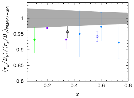
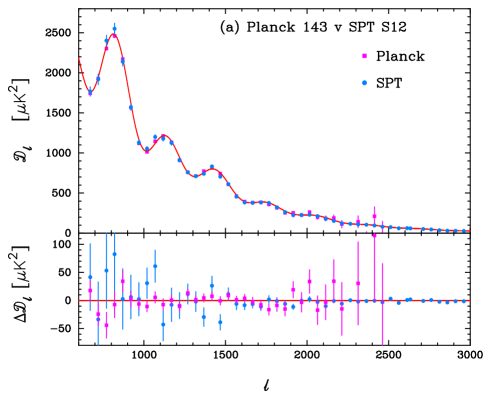
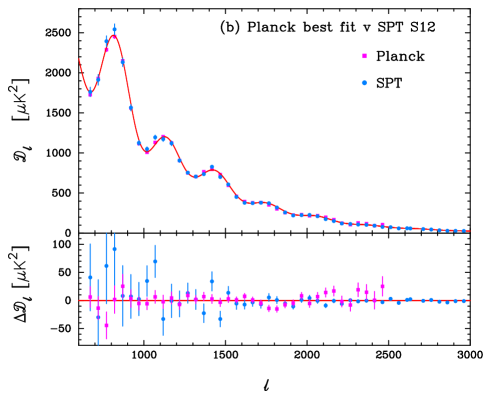
The parameter values derived from Planck for the base $\Lambda$CDM cosmology differ from those inferred by combining S12 with WMAP-7; e.g., the best-fit values of $H_{0}$ and $\Omega_{\Lambda}$ differ by $2.7\thinspace\sigma$ and $3.2\thinspace\sigma$ respectively, where $\sigma$ is the uncertainty in the WMAP-7+S12 determination. Furthermore, in Hou et al. (2012, herefter H12, a companion paper to S12) a trend in the S12 band-powers was identifed relative to the best-fit base $\Lambda$CDM spectrum, which they tentatively reported as evidence for new physics. This again differs from the results of Sect. 6, in which we found that the Planck data provide no evidence for any new physics beyond that incorporated in the base $\rm{\Lambda CDM}$ model. The purpose of this appendix is to investigate (as far as we can) the origin of these parameter differences and to comment on the trend identified in H12 in light of the more precise data we now have from Planck.

Note that the S12 result extends the earlier work of K11 (a subset of which is used in the highL data combination in the main body of this paper) from an analysis of $790\thinspace{\rm deg}^{2}$ of sky to a total field area of $2540\thinspace{\rm deg}^{2}$. S12 and H12 present constraints on the base $\rm{\Lambda CDM}$ model and extensions. Certain extended models are favoured when WMAP-7 and S12 are combined. For example, a running spectral index is favoured over a constant spectral index at the $2.2\thinspace\sigma$ level.

The differences between the S12 and Planck base $\rm{\Lambda CDM}$ cosmologies lead to different types of tension with non-CMB data. Whereas Planck is consistent to high precision with the BAO data (see Fig. 15) and shows some tension with the Riess et al. (2011) measurement of $H_{0}$, the WMAP-7+S12 best-fit cosmology is consistent with the $H_{0}$ measurement but in tension with the BAO measurements. The latter point is illustrated by Fig. 42, which is equivalent to Fig. 15 but uses the WMAP-7+SPT cosmology as a reference. All of the BAO measurements lie systematically low compared to the best-fit WMAP-7+S12 $\Lambda$CDM cosmology. This discrepancy was further motivation for the study in H12 of extensions to the standard cosmological model.

Appendix A shows that the Planck and WMAP-9 power spectra are in good agreement with each other after correction for a multiplicative calibration factor, and lead to closely similar cosmological parameters when the Planck likelihood is restricted to multipoles less than $1000$. A systematic difference between Planck and WMAP-7 band-powers is therefore not the cause of the discrepancy between the Planck and WMAP-7+S12 cosmologies. Alternative explanations might involve a systematic difference between the Planck and S12 band-powers at high multipoles, or a systematic problem related to the matching of the SPT and WMAP spectra, i.e., with their relative calibration.

We consider first a comparison of the Planck and S12 spectra. Since these spectra have a large overlap range at high multipoles, where both experiments have high signal-to-noise, there is no need to use WMAP as an intermediary to establish a relative calibration. We can compare the spectra directly via a joint likelihood analysis using the same foreground model that is used in the main body of this paper. Since the S12 spectrum is measured at a frequency of 150 GHz, we first present results using only the Planck $143\times 143$ GHz spectrum in the Planck likelihood. This reduces sensitivity to the details of the foreground modelling. Apart from small colour corrections, the foregrounds are identical, except for differences in the Poisson point source amplitudes.

Absolute calibration of the SPT spectra is determined by comparing with the WMAP-7 spectrum in the multipole range $600\leq\ell\leq 1000$. Since the spectra from both experiments are noisy in this multipole range, there is a large (roughly 3% in power) uncertainty in the absolute calibration of the S12 data. Here we use a version of the SPT S12 likelihood that does not include marginalization over calibration uncertainties. Instead, we self-consistently solve for a map calibration factor $y^{\rm SPT}_{150}$ between SPT and Planck. (This differs from the analyses of S12, H12 and Calabrese et al. 2013, which use an SPT covariance matrix that includes marginalization over calibration errors, and combine with other experiments without solving for a relative calibration factor.)

The results are shown in Fig. 43 (a). The agreement between the two sets of band-powers is most easily seen in the lower panel in which the best-fit model has been subtracted. The best-fit calibration factor is $y^{\rm SPT}_{150}=0.995$, well within the prior 1.3% calibration uncertainty. The model with minimum $\chi^{2}$ in this joint analysis has $\chi^{2}_{\rm SPT}=55.7$. To quantify the probability to exceed (PTE) this value of $\chi^{2}$ we need to determine the effective number of degrees of freedom. The SPT data have 47 band-powers and only two parameters that were heavily influenced by them: the Poisson point source amplitude and $y^{\rm SPT}_{150}$. Taking 45 as the number of degrees of freedom, we find a PTE of 13%.

Figure 44: A number of separate effects contribute to the difference in $H_{0}$ inferred from WMAP-7+S12 (top of left panel) and $H_{0}$ inferred from Planck+WP (bottom of left panel), all going in the same direction. These include assumptions about neutrino masses, calibration procedures, differences between WMAP-7 and WMAP-9, and differences in the relative calibrations between SPT and WMAP (as explained in the text). The right panel shows calibration parameter priors (top lines of each pair) and posteriors (bottom lines of each pair). The tighter of the priors shown for WMAP-7+S12, and that shown for WMAP-9+S12, come from using Planck to provide the relative calibration between WMAP and S12. We plot only the posterior for the Planck+S12 relative calibration. Note that the relative-calibration parameter $y^{\rm SPT}_{\rm X}$ is between S12 and the other indicated data set (i.e., WMAP or Planck).

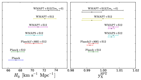
We find similar results when we combine the S12 likelihood with the full Planck+WP+highL likelihood. This is illustrated in Fig. 43 (b). Note that the Planck spectrum sits high compared to the best-fit spectrum at $\ell\ga 2300$, but in this region of the spectrum foreground and beam errors become significant and introduce large correlations between the data points. We find a minimum $\chi^{2}$ value of $\chi^{2}_{\rm SPT}=56.3$ for the best-fit cosmological model. Again assuming 45 degrees of freedom we find a PTE of 12%. Based on these $\chi^{2}$ values, we see no evidence of any inconsistency between the S12 band-powers and the best-fit Planck cosmological model. The parameter values for the Planck+S12 fits are listed in Table 13. We also include the parameter values from our own WMAP-9+S12 analysis. In this latter case, we do not include Planck-based (re)calibrations of WMAP or SPT, but allow the relative calibration between SPT and WMAP ($y_{150}^{\rm SPT/WMAP}$) to vary.

If the Planck and SPT power spectra are broadly consistent with each other, then why do the WMAP-7+S12 and Planck $\Lambda$CDM parameter estimates differ by so much? The bulk of the difference can be captured by just one parameter, which we choose here as $H_{0}$. The shifts in other parameters are highly correlated with the shift in $H_{0}$.

Some factors contributing to the difference in $H_{0}$ are summarized in Fig. 44. We start at the top with the WMAP-7+S12 result, which assumed zero neutrino mass. Progressing downwards in the plot, we have repeated the WMAP-7+S12 analysis assuming a neutrino mass of $0.06\thinspace{\rm eV}$ as in the Planck analysis described here. This lowers $H_{0}$ slightly. A further reduction in $H_{0}$ comes from using the Planck data to reduce the uncertainty in the WMAP-SPT relative calibration. By combining the Planck-WMAP 1.3% rescaling (see Appendix A) and the Planck-S12 calibration, we can place a tight prior on the WMAP-7-S12 relative calibration. Fig. 44 shows that this prior is roughly $1.5\thinspace\sigma$ higher than the posterior from the WMAP-7+S12 chain that uses the nominal S12 calibration. Switching from WMAP-7+S12 to WMAP-9+S12, in the next step in our progression, we again see a small shift to lower $H_{0}$, with $H_{0}=(70.4\pm 1.6)\thinspace{\rm km}\thinspace{\rm s}^{-1}\thinspace{\rm Mpc}^{-1}$. This latter value is very similar to that obtained if we replace the WMAP-9 data with the Planck+WP likelihood limited to $\ell_{\rm max}=800$ (as shown in Fig. 44). The Planck+S12 results plotted in Fig. 44 are from the last column of Table 13.

Each of the changes described above brings the base $\rm{\Lambda CDM}$ cosmological parameter values from SPT closer to those derived from Planck. Our results suggest that part of the discrepancy between the WMAP-7+S12 and Planck parameters arises from difficulties in self-consistently matching the SPT to the WMAP power spectra over a limited range of multipoles. This illustrates the advantages of having a single experiment, such as Planck, covering both low and high multipoles.

Table 13: Parameter constraints in $\Lambda$CDM models for various likelihood combinations as described in the text. The WMAP nine-year polarization likelihood is used in all of these fits. For Planck and SPT we use the standard foreground model, as described in Sect. 4. For WMAP, we follow the foreground treatment in Appendix A, removing only a Poisson-like term from the power spectrum. The last row of the table lists the SPT $\chi^{2}$ value for the best-fit parameters ($47$ data points).

      WMAP-9+S12       Planck 143+S12       Planck+S12

Parameter       68% limit       68% limit       68% limit

$$100\Omega_{\rm b}h^{2}$$.                     

.                     

.                     

.                     

.                     

.                     

.                     

.                     

.                     

.                     

.                     

Appendix C Dependence of cosmological parameters in extended models on foreground modelling and likelihood choices

A large number of likelihood comparison tests on parameters in the base $\Lambda$CDM cosmology are discussed in Planck Collaboration XV (2014). In the main body of this paper, we report constraints on a wide variety of extended models. In many of these models the cosmological parameters are strongly degenerate with each other and are therefore more sensitive to the detailed modelling of foregrounds, frequency choices, and likelihood methodology. In this Appendix we discuss briefly how one-parameter extensions of the $\Lambda$CDM model are affected by various choices.

C.1 Impact of foreground priors

Throughout this paper we have used a particular parameterization of the foreground model, and marginalized over the free parameters using relatively wide priors. As discussed in Sect. 4, the choice of these priors is subjective and was guided by theoretical expectations and by other data, particularly results from high-resolution CMB experiments and the early Planck analysis of the CIB power spectrum (Planck Collaboration XVIII 2011). As discussed in Sect. 4, for Planck the dominant foregrounds are the Poisson contributions from unresolved point sources and the clustered CIB component at $217\thinspace$GHz. The other components are of much lower amplitude and poorly constrained by Planck data alone.

For the thermal and kinetic SZ amplitudes we have imposed uniform priors of $0\leq A^{\mathrm{tSZ}}\leq 10$ and $0\leq A^{\mathrm{kSZ}}\leq 10$. These priors have little impact on the parameters derived for the base $\Lambda$CDM model, or on the parameters of extended cosmologies if Planck is combined with ACT and SPT data at high multipoles. However, for extended cosmologies the priors on these ‘minor’ components do have a small impact on the cosmological parameters. Table 14 gives results obtained from doubling the width of the SZ priors. The constraints on the extended parameters change by small amounts compared to the Planck+WP entries in Table  10, giving an impression of the sensitivity of Planck+WP numbers to minor foregrounds.

The use of additional high-$\ell$ CMB data to constrain the foreground parameters depends on having a foreground model that can reliably extrapolate between the scales relevant for Planck and the smaller scales where the high-resolution experiments have the tightest constraints. As a simple test of the model used in the main body of the paper, we relax here our assumption that the CIB spectral index is constant with a Gaussian prior $\gamma^{\rm CIB}=0.7\pm 0.2$. Any change in CIB index between small and larger scales could lead to a bias in the foreground model subtracted from the Planck spectra, particularly in the $217\times 217\thinspace\mathrm{GHz}$ spectrum where the CIB is the dominant foreground component. However, as shown in Fig. 45, and Table 14, the inferred cosmological parameters are actually extremely insensitive to the details of the model, with very similar results obtained with no $\gamma^{\rm CIB}$ prior and allowing a free running of the spectral index through the parameter $d\gamma^{\mathrm{CIB}}/d\ln\ell$. (Note that we have assumed here that the $\ell$-dependence of the CIB is the same, up to an amplitude, at the different frequencies.) The interpretation of the foregrounds does change significantly, and indeed there is mild evidence for running of the CIB spectral index, but it has almost no impact on the cosmology. This should not be too surprising, since the CIB signal is frequency-dependent unlike the cosmological signal, but nonetheless it is reassuring that degeneracies with, for example, the SZ amplitudes do not indirectly cause biases in cosmological parameters.

Figure 45: Comparison of parameter constraints from Planck+WP+highL for three CIB foreground models with different restrictions on the CIB spectral index $\gamma^{\rm CIB}$ (assumed to be the same in the $143$ and $217\thinspace\mathrm{GHz}$ channels). The top six panels show cosmological parameter constraints on $n_{\rm s}$ (top left) in the base $\Lambda$CDM model and on single-parameter extensions of the $\Lambda$CDM model. These are very stable to the modelling of the CIB. Each sub-plot is obtained from an independent analysis of that model with CosmoMC. The lower six panels show the constraints on a subset of the foreground parameters in the base $\Lambda$CDM model, some of which change significantly.

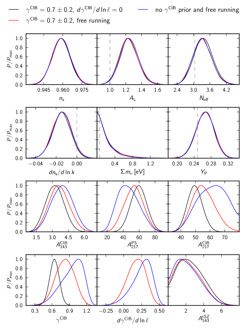
We have not investigated extensively the impact of varying the tSZ and kSZ templates. A variety of different approaches (analytic, semi-analytic and numerical) have been used to estimate tSZ templates (e.g., Komatsu & Seljak 2002; Shaw et al. 2010; Sehgal et al. 2010; Trac et al. 2011; Battaglia et al. 2010, 2012). These have similar shapes at multipoles $\ell\la 3000$, relevant to Planck and to the tSZ template used here. The shape of our template is also a good match to the power spectrum of the Planck Compton-$y$ map over the multipole range $100\la\ell\la 1000$ (Planck Collaboration XXI 2014). The normalization of the tSZ templates (i.e., their dependence on $\sigma_{8}$) and their shapes at multipoles $\ell\ga 3000$, depend on uncertain gas physics (including energy injection from AGN). For this reason, we have not attempted to link the amplitude of the tSZ template to the amplitude of the matter power spectrum in the parameter analyses. The tSZ template used here is similar in shape to the Battaglia et al. (2010) template that has been used extensively in the analysis of ACT and SPT data. The effects of varying tSZ and kSZ templates on high-resolution CMB experiments have been investigated by Dunkley et al. (2011), Reichardt et al. (2012), and Dunkley et al. (2013) who find very little effect on cosmological parameters.

Table 14: Constraints on one-parameter extensions of the $\Lambda$CDM model from Planck with various likelihood variations. Planck+WP+highL is used in all cases except for the column listing results for $\tau=0.07\pm 0.013$, where the WMAP polarization likelihood is replaced by this $\tau$ prior, and the ninth column, which does not include the high-$\ell$ experiments and doubles the default width of the flat priors on the two SZ amplitudes $A^{\mathrm{tSZ}}$ and $A^{\mathrm{kSZ}}$. The running CIB model has no prior on $\gamma^{\mathrm{CIB}}$ and allows for spectral curvature through the parameter $d\gamma^{\mathrm{CIB}}/d\ln\ell$. The final column in the table shows the results of modelling a small systematic feature in the $217\times 217\thinspace{\rm GHz}$ spectrum, as described in Sect. C.4.

CamSpec Plik $$l_{\text{max}}=2000$$ no Running CIB 217 systematic

Parameter 95% limits 95% limits 95% limits 95% limits 95% limits 95% limits 95% limits 95% limits 95% limits

.

.

.

.

.

C.2 WMAP low-$\ell$ polarization likelihood

The large-scale polarization from nine years of WMAP observations (Bennett et al. 2012) provides our most powerful constraint on the reionization optical depth $\tau$. As shown in Sect. 3 it is not essential to use WMAP polarization information to obtain tight constraints on cosmological parameters from Planck. Using WMAP does, however, improve the constraints on the amplitude of the power spectrum and, via the partial parameter degeneracies sensitive to the relative amplitude of large and small-scale power and the amount of lensing, WMAP polarization also has an impact on other cosmological parameters. Most directly, since the small-scale CMB power scales roughly with $e^{-2\tau}\sigma_{8}^{2}$, the inferred value of $\sigma_{8}$ is approximately proportional to $e^{\tau}$ as discussed in Sect. 3.4.

The polarization measurement at low multipoles is challenging because of the high level of polarized Galactic foregrounds, so it is important to assess the impact if the assumed constraint were slightly wrong. Figure 46 shows how cosmological parameters shift if instead of using WMAP polarization we impose a prior $\tau=0.07\pm 0.013$ ($1\sigma$), which is about the same width but about $0.02$ lower than the posterior obtained from WMAP (as for example might be obtained if there were some residual foreground contamination or instrument systematic). Table. 14 shows the corresponding impact on parameter constraints with high-$\ell$ CMB data added to Planck. The shifts are consistent with the known parameter degeneracies, and the $\Lambda$CDM constraints on $\sigma_{8}$ would shift downwards by a factor of approximately $e^{0.02}$, or about $2\%$. For this reason, in Sect. 3.4 we have quoted a constraint on $e^{-\tau}\sigma_{8}$, which is insensitive to possible errors in the large-scale polarization likelihood. A change in the Planck calibration would also have a similar direct effect on the inferred physical amplitudes.

Figure 46: Effect on cosmological parameter constraints of replacing the WMAP low-$\ell$ polarization likelihood with a prior of $\tau=0.07\pm 0.013$, which prefers lower values of the optical depth. The top-left sub-plot is $n_{\rm s}$ in the base $\Lambda$CDM model, while the others are for one-parameter extensions. Each sub-plot shows results from independent CosmoMC analyses of the corresponding model.

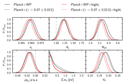
C.3 Planck likelihood

The results of this paper are based on the CamSpec likelihood, which includes information from 100, 143 and $217\thinspace\mathrm{GHz}$ channels, with a range of multipole cuts as reviewed briefly in Sect. 2.3 and summarized in Table 6. The combination of channels used allows a number of foreground parameters to be partially determined from Planck data alone, and as discussed in Sect. 4 the foreground parameters can be determined more precisely by including additional information from other high-$\ell$ data sets. Planck Collaboration XV (2014) discusses and compares the CamSpec likelihood with an alternative cross- and auto-spectrum likelihood, Plik. The Plik likelihood uses identical masks over the frequency range $100$–$217\thinspace\mathrm{GHz}$ (retaining $48\%$ of the sky), ignores correlations between multipoles and uses different assumptions to estimate instrument noise and to correct for Galactic dust, as described in Planck Collaboration XV (2014). For the base $\Lambda$CDM model, these two likelihood codes give almost identical results. In this section, we investigate briefly how cosmological parameters in extended $\Lambda$CDM models vary between the two likelihood codes and for some data cuts in the CamSpec likelihood.

Figure 47: Upper: comparison of the $\Lambda$CDM constraints on $n_{\rm s}$ (top-left) and single-parameter extensions of the $\Lambda$CDM model for a variety of data cuts for Planck+WP. Each sub-plot is obtained from a separate CosmoMC analysis of the corresponding model. The dashed lines show the results from Plik, an alternative likelihood discussed in  Planck Collaboration XV (2014), run here with the same SZ and CIB foreground priors as for the CamSpec results. For the extended models, the value of the additional parameter in the base $\Lambda$CDM model is shown with the vertical dashed lines. Lower: same as the upper set of panels, but for Planck+WP+highL. Additional data from the high-$\ell$ CMB experiments significantly reduce the foreground degeneracies.

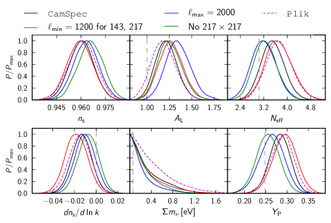
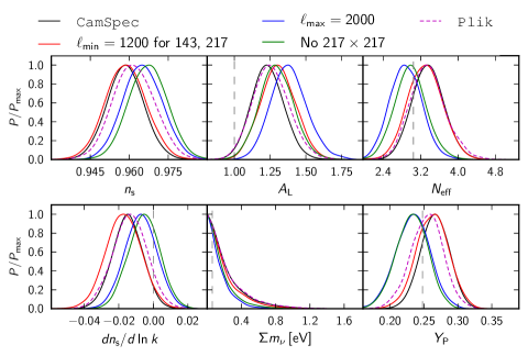
The results are summarized in Fig. 47 and Table 14. Shifts in parameter values are expected, since different combinations of data are being used and hence have differing amounts of noise and cosmic variance. With fewer frequencies overlapping at any angular scale, the foreground parameters are less well determined, and any degeneracies with foreground parameters are expected to open up. Fig. 47 shows that there are noticeable shifts in parameter values, but when also including additional high-$\ell$ CMB data, which constrain the foreground parameters to higher precision, the relatively small differences between CamSpec and Plik are significantly reduced. The two likelihood codes agree well, even for extended models when the high-$\ell$ CMB data are added to the likelihoods.

However, the preference from the temperature power spectrum for $A_{\rm L}>1$ actually becomes stronger on adding high-$\ell$ data. Reducing $\ell_{\rm max}$ to $2000$ in the CamSpec likelihood also shifts $A_{\rm L}$ to higher values, particularly with the addition of the high-$\ell$ data. We do not, at this stage, have a full understanding of these shifts in $A_{\rm L}$. We note that the high-$\ell$ ACT data itself favours high $A_{\rm L}$ (Sievers et al. 2013), and this may be part of the reason behind the shift to high values when high-$\ell$ data are included. (The truncation of Planck spectra at $l_{\text{max}}=2000$ also limits the accuracy of matching high-$\ell$ data to Planck. There is then no overlapping multipole range with the SPT data and a significantly narrower overlap range for ACT.)

The analysis of extended $\Lambda$CDM models with strong parameter degeneracies is complex and sensitive to small systematic errors in the CMB data and to errors in the foreground model. In the analysis of extended models we have usually quoted results from the Planck+WP+highL data combination, using the full CamSpec likelihood. With this combination, we utilize the high signal-to-noise ratio of the Planck spectra at $143$ and $217\thinspace\mathrm{GHz}$, which have a wide multipole range with which to match high-$\ell$ experiments to Planck, and gain better control of foregrounds via the inclusion of high-$\ell$ data. The general “rule of thumb” adopted in this paper has been to use the differences between parameter constraints from Planck+WP and Planck+WP+highL as a guide to whether parameters are sensitive to errors in the foreground model (or other sources of error). We do sometimes see shifts of up to around $1\thinspace\sigma$ between these likelihoods in the parameter values for extended models and this needs to be borne in mind when interpreting our results. In the absence of any additional information, we take the cosmological parameters from Planck+WP+highL as our best estimates for extended models.

C.4 $217\thinspace{\rm GHz}$ systematic feature

As discussed in Sect. 1, following the submission of the Planck 2013 papers, we discovered strong evidence that a small dip in the $217\times 217\thinspace{\rm GHz}$ spectrum at $\ell\approx 1800$ varies between surveys and is a systematic feature caused by incomplete subtraction of $4\thinspace{\rm K}$ cooler lines from the time-ordered data. To estimate the impact of such a systematic on cosmology, we test the sensitivity of our results to adding a dip in the $217\times 217\thinspace{\rm GHz}$ spectrum in the range $1700\leq\ell\leq 1860$, which we model as

$$\Delta\mathcal{D}_{\ell}^{217\times 217}=-W\sin\left(\frac{(\ell-1700)\pi}{160}\right).$$ (112)

(Note that the tests described in this section were done before the submission of the 2013 papers.) Here, $W$ is a free amplitude parameter that we marginalize over using a flat prior. For the base $\rm{\Lambda CDM}$ model we find $W=(26\pm 5)\thinspace\mu{\rm K}^{2}$ (Planck+WP), and hence a significant (but highly a posteriori) dip amplitude is strongly preferred by the data, consistent with a systematic effect. The impact on the cosmological parameters is small, but not negligible, typically causing shifts of below $0.5\thinspace\sigma$. Marginalizing over the dip amplitude $W$ raises the mean $H_{0}$ in the base model by approximately $0.3\thinspace\sigma$, and gives comparable small shifts to one-parameter extensions, as summarized in the final column (labelled “217 systematic”) of Table 14. Marginalizing over $W$ does not significantly change the marginalized value of $A_{\rm L}$.

In summary, the $\ell=1800$ dip in the $217\times 217\thinspace{\rm GHz}$ spectrum has a non-negligible, but small, impact on cosmological parameters, even for extensions to the base $\rm{\Lambda CDM}$ model. The impact on cosmological parameters is typically less than $0.5\thinspace\sigma$, comparable to the shifts caused by uncertainties in the modelling of unresolved foregrounds. However, tests designed to search for localized features in the Planck power spectrum can respond strongly to the systematic effect, as reported in Planck Collaboration XXII (2014). Users of the Planck likelihood should bear this in mind.