22institutetext: Aalto University Metsähovi Radio Observatory, Metsähovintie 114, FIN-02540 Kylmälä, Finland
33institutetext: African Institute for Mathematical Sciences, 6-8 Melrose Road, Muizenberg, Cape Town, South Africa
44institutetext: Agenzia Spaziale Italiana Science Data Center, c/o ESRIN, via Galileo Galilei, Frascati, Italy
55institutetext: Agenzia Spaziale Italiana, Viale Liegi 26, Roma, Italy
66institutetext: Astrophysics Group, Cavendish Laboratory, University of Cambridge, J J Thomson Avenue, Cambridge CB3 0HE, U.K.
77institutetext: Astrophysics & Cosmology Research Unit, School of Mathematics, Statistics & Computer Science, University of KwaZulu-Natal, Westville Campus, Private Bag X54001, Durban 4000, South Africa
88institutetext: Atacama Large Millimeter/submillimeter Array, ALMA Santiago Central Offices, Alonso de Cordova 3107, Vitacura, Casilla 763 0355, Santiago, Chile
99institutetext: CITA, University of Toronto, 60 St. George St., Toronto, ON M5S 3H8, Canada
1010institutetext: CNRS, IRAP, 9 Av. colonel Roche, BP 44346, F-31028 Toulouse cedex 4, France
1111institutetext: California Institute of Technology, Pasadena, California, U.S.A.
1212institutetext: Centre for Theoretical Cosmology, DAMTP, University of Cambridge, Wilberforce Road, Cambridge CB3 0WA U.K.
1313institutetext: Centro de Estudios de Física del Cosmos de Aragón (CEFCA), Plaza San Juan, 1, planta 2, E-44001, Teruel, Spain
1414institutetext: Computational Cosmology Center, Lawrence Berkeley National Laboratory, Berkeley, California, U.S.A.
1515institutetext: Consejo Superior de Investigaciones Científicas (CSIC), Madrid, Spain
1616institutetext: DSM/Irfu/SPP, CEA-Saclay, F-91191 Gif-sur-Yvette Cedex, France
1717institutetext: DTU Space, National Space Institute, Technical University of Denmark, Elektrovej 327, DK-2800 Kgs. Lyngby, Denmark
1818institutetext: Département de Physique Théorique, Université de Genève, 24, Quai E. Ansermet,1211 Genève 4, Switzerland
1919institutetext: Departamento de Física Fundamental, Facultad de Ciencias, Universidad de Salamanca, 37008 Salamanca, Spain
2020institutetext: Departamento de Física, Universidad de Oviedo, Avda. Calvo Sotelo s/n, Oviedo, Spain
2121institutetext: Department of Astronomy and Astrophysics, University of Toronto, 50 Saint George Street, Toronto, Ontario, Canada
2222institutetext: Department of Astrophysics/IMAPP, Radboud University Nijmegen, P.O. Box 9010, 6500 GL Nijmegen, The Netherlands
2323institutetext: Department of Electrical Engineering and Computer Sciences, University of California, Berkeley, California, U.S.A.
2424institutetext: Department of Physics & Astronomy, University of British Columbia, 6224 Agricultural Road, Vancouver, British Columbia, Canada
2525institutetext: Department of Physics and Astronomy, Dana and David Dornsife College of Letter, Arts and Sciences, University of Southern California, Los Angeles, CA 90089, U.S.A.
2626institutetext: Department of Physics and Astronomy, University College London, London WC1E 6BT, U.K.
2727institutetext: Department of Physics, Gustaf Hällströmin katu 2a, University of Helsinki, Helsinki, Finland
2828institutetext: Department of Physics, Princeton University, Princeton, New Jersey, U.S.A.
2929institutetext: Department of Physics, University of California, Berkeley, California, U.S.A.
3030institutetext: Department of Physics, University of California, One Shields Avenue, Davis, California, U.S.A.
3131institutetext: Department of Physics, University of California, Santa Barbara, California, U.S.A.
3232institutetext: Department of Physics, University of Illinois at Urbana-Champaign, 1110 West Green Street, Urbana, Illinois, U.S.A.
3333institutetext: Dipartimento di Fisica e Astronomia G. Galilei, Università degli Studi di Padova, via Marzolo 8, 35131 Padova, Italy
3434institutetext: Dipartimento di Fisica e Scienze della Terra, Università di Ferrara, Via Saragat 1, 44122 Ferrara, Italy
3535institutetext: Dipartimento di Fisica, Università La Sapienza, P. le A. Moro 2, Roma, Italy
3636institutetext: Dipartimento di Fisica, Università degli Studi di Milano, Via Celoria, 16, Milano, Italy
3737institutetext: Dipartimento di Fisica, Università degli Studi di Trieste, via A. Valerio 2, Trieste, Italy
3838institutetext: Dipartimento di Fisica, Università di Roma Tor Vergata, Via della Ricerca Scientifica, 1, Roma, Italy
3939institutetext: Dipartimento di Matematica, Università di Roma Tor Vergata, Via della Ricerca Scientifica, 1, Roma, Italy
4040institutetext: Discovery Center, Niels Bohr Institute, Blegdamsvej 17, Copenhagen, Denmark
4141institutetext: Dpto. Astrofísica, Universidad de La Laguna (ULL), E-38206 La Laguna, Tenerife, Spain
4242institutetext: European Southern Observatory, ESO Vitacura, Alonso de Cordova 3107, Vitacura, Casilla 19001, Santiago, Chile
4343institutetext: European Space Agency, ESAC, Planck Science Office, Camino bajo del Castillo, s/n, Urbanización Villafranca del Castillo, Villanueva de la Cañada, Madrid, Spain
4444institutetext: European Space Agency, ESTEC, Keplerlaan 1, 2201 AZ Noordwijk, The Netherlands
4545institutetext: Finnish Centre for Astronomy with ESO (FINCA), University of Turku, Väisäläntie 20, FIN-21500, Piikkiö, Finland
4646institutetext: Haverford College Astronomy Department, 370 Lancaster Avenue, Haverford, Pennsylvania, U.S.A.
4747institutetext: Helsinki Institute of Physics, Gustaf Hällströmin katu 2, University of Helsinki, Helsinki, Finland
4848institutetext: INAF - Osservatorio Astronomico di Padova, Vicolo dell’Osservatorio 5, Padova, Italy
4949institutetext: INAF - Osservatorio Astronomico di Roma, via di Frascati 33, Monte Porzio Catone, Italy
5050institutetext: INAF - Osservatorio Astronomico di Trieste, Via G.B. Tiepolo 11, Trieste, Italy
5151institutetext: INAF/IASF Bologna, Via Gobetti 101, Bologna, Italy
5252institutetext: INAF/IASF Milano, Via E. Bassini 15, Milano, Italy
5353institutetext: INFN, Sezione di Bologna, Via Irnerio 46, I-40126, Bologna, Italy
5454institutetext: INFN, Sezione di Roma 1, Università di Roma Sapienza, Piazzale Aldo Moro 2, 00185, Roma, Italy
5555institutetext: IPAG: Institut de Planétologie et d’Astrophysique de Grenoble, Université Joseph Fourier, Grenoble 1 / CNRS-INSU, UMR 5274, Grenoble, F-38041, France
5656institutetext: ISDC Data Centre for Astrophysics, University of Geneva, ch. d’Ecogia 16, Versoix, Switzerland
5757institutetext: IUCAA, Post Bag 4, Ganeshkhind, Pune University Campus, Pune 411 007, India
5858institutetext: Imperial College London, Astrophysics group, Blackett Laboratory, Prince Consort Road, London, SW7 2AZ, U.K.
5959institutetext: Infrared Processing and Analysis Center, California Institute of Technology, Pasadena, CA 91125, U.S.A.
6060institutetext: Institut Néel, CNRS, Université Joseph Fourier Grenoble I, 25 rue des Martyrs, Grenoble, France
6161institutetext: Institut Universitaire de France, 103, bd Saint-Michel, 75005, Paris, France
6262institutetext: Institut d’Astrophysique Spatiale, CNRS (UMR8617) Université Paris-Sud 11, Bâtiment 121, Orsay, France
6363institutetext: Institut d’Astrophysique de Paris, CNRS (UMR7095), 98 bis Boulevard Arago, F-75014, Paris, France
6464institutetext: Institute for Space Sciences, Bucharest-Magurale, Romania
6565institutetext: Institute of Astronomy and Astrophysics, Academia Sinica, Taipei, Taiwan
6666institutetext: Institute of Astronomy, University of Cambridge, Madingley Road, Cambridge CB3 0HA, U.K.
6767institutetext: Institute of Mathematics and Physics, Centre for Cosmology, Particle Physics and Phenomenology, Louvain University, Louvain-la-Neuve, Belgium
6868institutetext: Institute of Theoretical Astrophysics, University of Oslo, Blindern, Oslo, Norway
6969institutetext: Instituto de Astrofísica de Canarias, C/Vía Láctea s/n, La Laguna, Tenerife, Spain
7070institutetext: Instituto de Física de Cantabria (CSIC-Universidad de Cantabria), Avda. de los Castros s/n, Santander, Spain
7171institutetext: Jet Propulsion Laboratory, California Institute of Technology, 4800 Oak Grove Drive, Pasadena, California, U.S.A.
7272institutetext: Jodrell Bank Centre for Astrophysics, Alan Turing Building, School of Physics and Astronomy, The University of Manchester, Oxford Road, Manchester, M13 9PL, U.K.
7373institutetext: Kavli Institute for Cosmology Cambridge, Madingley Road, Cambridge, CB3 0HA, U.K.
7474institutetext: LAL, Université Paris-Sud, CNRS/IN2P3, Orsay, France
7575institutetext: LERMA, CNRS, Observatoire de Paris, 61 Avenue de l’Observatoire, Paris, France
7676institutetext: Laboratoire AIM, IRFU/Service d’Astrophysique - CEA/DSM - CNRS - Université Paris Diderot, Bât. 709, CEA-Saclay, F-91191 Gif-sur-Yvette Cedex, France
7777institutetext: Laboratoire Traitement et Communication de l’Information, CNRS (UMR 5141) and Télécom ParisTech, 46 rue Barrault F-75634 Paris Cedex 13, France
7878institutetext: Laboratoire de Physique Subatomique et de Cosmologie, Université Joseph Fourier Grenoble I, CNRS/IN2P3, Institut National Polytechnique de Grenoble, 53 rue des Martyrs, 38026 Grenoble cedex, France
7979institutetext: Laboratoire de Physique Théorique, Université Paris-Sud 11 & CNRS, Bâtiment 210, 91405 Orsay, France
8080institutetext: Lawrence Berkeley National Laboratory, Berkeley, California, U.S.A.
8181institutetext: Max-Planck-Institut für Astrophysik, Karl-Schwarzschild-Str. 1, 85741 Garching, Germany
8282institutetext: McGill Physics, Ernest Rutherford Physics Building, McGill University, 3600 rue University, Montréal, QC, H3A 2T8, Canada
8383institutetext: MilliLab, VTT Technical Research Centre of Finland, Tietotie 3, Espoo, Finland
8484institutetext: Niels Bohr Institute, Blegdamsvej 17, Copenhagen, Denmark
8585institutetext: Observational Cosmology, Mail Stop 367-17, California Institute of Technology, Pasadena, CA, 91125, U.S.A.
8686institutetext: Optical Science Laboratory, University College London, Gower Street, London, U.K.
8787institutetext: SB-ITP-LPPC, EPFL, CH-1015, Lausanne, Switzerland
8888institutetext: SISSA, Astrophysics Sector, via Bonomea 265, 34136, Trieste, Italy
8989institutetext: School of Physics and Astronomy, Cardiff University, Queens Buildings, The Parade, Cardiff, CF24 3AA, U.K.
9090institutetext: School of Physics and Astronomy, University of Nottingham, Nottingham NG7 2RD, U.K.
9191institutetext: Space Sciences Laboratory, University of California, Berkeley, California, U.S.A.
9292institutetext: Special Astrophysical Observatory, Russian Academy of Sciences, Nizhnij Arkhyz, Zelenchukskiy region, Karachai-Cherkessian Republic, 369167, Russia
9393institutetext: Stanford University, Dept of Physics, Varian Physics Bldg, 382 Via Pueblo Mall, Stanford, California, U.S.A.
9494institutetext: Sub-Department of Astrophysics, University of Oxford, Keble Road, Oxford OX1 3RH, U.K.
9595institutetext: Theory Division, PH-TH, CERN, CH-1211, Geneva 23, Switzerland
9696institutetext: UPMC Univ Paris 06, UMR7095, 98 bis Boulevard Arago, F-75014, Paris, France
9797institutetext: Université de Toulouse, UPS-OMP, IRAP, F-31028 Toulouse cedex 4, France
9898institutetext: University of Granada, Departamento de Física Teórica y del Cosmos, Facultad de Ciencias, Granada, Spain
9999institutetext: University of Miami, Knight Physics Building, 1320 Campo Sano Dr., Coral Gables, Florida, U.S.A.
100100institutetext: Warsaw University Observatory, Aleje Ujazdowskie 4, 00-478 Warszawa, Poland
Planck 2013 results. XV. CMB power spectra and likelihood
This paper presents the Planck likelihood, a complete statistical description of the two-point correlation function of the CMB temperature fluctuations that accounts for all known relevant uncertainties, both instrumental and astrophysical in nature. We use this likelihood to derive our best estimate of the CMB angular power spectrum from Planck over three decades in multipole moment, , covering . The main source of error at is cosmic variance. Uncertainties in small-scale foreground modelling and instrumental noise dominate the error budget at higher s. For , our likelihood exploits all Planck frequency channels from 30 to 353 GHz, separating the cosmological CMB signal from diffuse Galactic foregrounds through a physically motivated Bayesian component separation technique. At , we employ a correlated Gaussian likelihood approximation based on a fine-grained set of angular cross-spectra derived from multiple detector combinations between the 100, 143, and 217 GHz frequency channels, marginalizing over power spectrum foreground templates. We validate our likelihood through an extensive suite of consistency tests, and assess the impact of residual foreground and instrumental uncertainties on the final cosmological parameters. We find good internal agreement among the high- cross-spectra with residuals below a few at , in agreement with estimated calibration uncertainties. We compare our results with foreground-cleaned CMB maps derived from all Planck frequencies, as well as with cross-spectra derived from the 70 GHz Planck map, and find broad agreement in terms of spectrum residuals and cosmological parameters. We further show that the best-fit cosmology is in excellent agreement with preliminary Planck and polarisation spectra. We find that the standard cosmology is well constrained by Planck from the measurements at . One specific example is the spectral index of scalar perturbations, for which we report a deviation from scale invariance, . Increasing the multipole range beyond does not increase our accuracy for the parameters, but instead allows us to study extensions beyond the standard model. We find no indication of significant departures from the framework. Finally, we report a tension between the Planck best-fit CDM model and the low- spectrum in the form of a power deficit of 5–10% at , with a statistical significance of 2.5–3. Without a theoretically motivated model for this power deficit, we do not elaborate further on its cosmological implications, but note that this is our most puzzling finding in an otherwise remarkably consistent dataset.
Key Words.:
Cosmology: cosmic background radiation – Surveys – Methods: data analysis1 Introduction
This paper, one of a set associated with the 2013 release of data from the Planck111Planck (http://www.esa.int/Planck) is a project of the European Space Agency (ESA) with instruments provided by two scientific consortia funded by ESA member states (in particular the lead countries France and Italy), with contributions from NASA (USA) and telescope reflectors provided by a collaboration between ESA and a scientific consortium led and funded by Denmark.mission (Planck Collaboration I 2013), describes the CMB power spectra and the likelihood that we derive from the Planck data.
The power spectrum of the Cosmic Microwave Background (CMB) is a unique signature of the underlying cosmological model (e.g., Spergel et al. 2003; Hinshaw et al. 2012). It has been measured over the whole sky by COBE and WMAP, and over smaller regions by ground-based and sub-orbital experiments (e.g., Tristram et al. 2005; Jones et al. 2006; Reichardt et al. 2009; Fowler et al. 2010; Das et al. 2011; Keisler et al. 2011; Story et al. 2012; Das et al. 2013). By mapping the whole sky to scales of a few arcminutes, Planck now measures the power spectrum over an unprecedented range of scales from a single experiment. To estimate cosmological parameters from the power spectrum requires a likelihood function that propagates uncertainties.
In this paper we describe the power spectra obtained from the Planck temperature data, as well as the associated likelihood function. Since the probability distribution of the power spectrum is non-Gaussian at large scales, we follow a hybrid approach to construct the likelihood (Efstathiou 2004, 2006), using a Gibbs sampling based approach at low multipoles, , and a pseudo-Cℓ technique at high multipoles (Hivon et al. 2002).
The high- part of the Planck likelihood is based on power spectra estimated from each Planck detector in the frequency range 100 to 217 GHz, allowing careful assessment of each detector’s response to the sky emission. We implement two independent likelihood methods. The first, used in the distributed likelihood code, estimates the power spectrum at every multipole, together with the associated covariance matrix. The second takes a simplified form, binning the spectra, and is used to explore the stability of the results with respect to different instrumental and astrophysical systematic effects. The methods give consistent results.
Unresolved extragalactic foregrounds make a significant contribution to the power spectra at high multipoles. We develop a model for these foregrounds, designed to allow the Planck likelihood to be combined with high resolution data from the Atacama Cosmology Telescope (ACT) and the South Pole Telescope (SPT). We combine frequencies and model unresolved foregrounds in a physical way, as in e.g., Shirokoff et al. (2010); Dunkley et al. (2011); Reichardt et al. (2012), performing component separation at small scales at the power spectrum level. On large scales, , Galactic contamination is more significant. We use the Planck temperature maps in the range GHz to separate Galactic foregrounds in the maps, and then estimate the full probability distribution of the CMB power spectrum.
2 High- likelihoods
The Planck maps consist of the order pixels for each detector, so a likelihood described directly at the pixel level would be too time consuming. A significant compression of data can be achieved with minimal information loss using pseudo- power spectra, even in the case of incomplete sky coverage. Here we describe the form of the likelihood function of the compressed data, given a sky signal and instrumental model.
Following Hamimeche & Lewis (2008), we assume a Gaussian form of the likelihood based on pseudo-spectra that have been corrected to account for partial sky masking. We use a ‘fine-grained’ data description, computing spectra of maps from individual detectors or detector sets. Table 1 describes the 13 maps used in the analysis, spanning 100 to 217 GHz. We compute the spectra at these multiple frequencies to simultaneously constrain the CMB and foreground contributions. We choose these frequencies as a trade-off between adding further information, and adding further complexity to the foreground model, which would be needed to including the adjacent 70 and 353 GHz channels (see Sect. 3 for further discussion). In our baseline analysis the spectra are computed at each multipole, together with an estimate of the full covariance matrix with off-diagonal errors between different spectra and multipoles. As in the WMAP analysis, we use only cross-spectra between detectors, alleviating the need to accurately model the mean noise contribution.
|
In this section, we begin with a reminder of the pseudo-spectrum approach, and describe our baseline likelihood distribution, hereafter referred to as the CamSpec likelihood. We then show how a compression of spectra within a given frequency can be achieved with negligible loss of information. We describe the signal and instrument model, including detector noise properties, calibration, and beam uncertainties.
Next, we describe an alternative, simpler, form of the likelihood, hereafter referred to as Plik, based on binned power spectra with an inverse-Wishart distribution. This does not require the pre-computation of large covariance matrices, so changing the sky or instrument modeling is straightforward. This simpler form of the likelihood will be used to assess the robustness of our likelihood methodology with respect to technical choices and astrophysical foreground modeling.
In Sect. 7.5 we also compare these likelihoods to pseudo-spectra computed directly from CMB maps estimated by multi-frequency component separation (Planck Collaboration XII 2013).
2.1 The CamSpec likelihood
We define as the spherical harmonic coefficients of the weighted temperature map of detector . The pseudo-spectrum at multipole , for the detector pair is then given by
| (1) |
where the dagger, , denotes the Hermitian transpose. This is related to the ‘deconvolved’ spectrum, , by a coupling matrix,
| (2) |
For an isotropic signal on the sky, the ensemble average of these deconvolved spectra are equal to the spectra of the theoretical models (including CMB and isotropic unresolved foregrounds) that we wish to test. For completeness, the coupling matrices are given explicitly in Appendix A.1.
In the first method, CamSpec, we form the deconvolved spectra without any prior smoothing of the pseudo-spectra . Even for the largest sky masks used in our analysis (see Sect. 3), the coupling matrices are non-singular. The deconvolution requires the evaluation of coupling matrices for a data set with sky maps, which takes a moderate, but not excessive, amount of computer time.
A more challenging computational task is to compute the covariances of the pseudo-spectra, i.e., Here we need to compute coupling matrices, and the problem rapidly becomes computationally intractable even for relatively low values of . For the moment we will assume that these covariance matrices are available and describe their computation in Appendix A.4. We will use the notation to denote a column vector for which the index of a single element denotes the map combination () and multipole . We denote the covariance matrix of this vector as
| (3) |
As explained later, the deconvolved detector set cross-spectra given by Eq. 2 can be efficiently combined within a given frequency pair after a small effective recalibration, taking into account their respective isotropised beam transfer function and noise levels (see Appendix A.3 for the detailed procedure). Covariance estimates of these combined spectra can be deduced from those of the detector set cross-spectra. The covariance matrix is computed for a fixed fiducial model, and we approximate the likelihood as a Gaussian, described in Appendix A.5. The likelihood thus takes the form with
For the current analysis we include the following (deconvolved) spectrum combinations,
| (4) |
coupled to a parametric model of the CMB and foreground power spectra. The multipole ranges we select depend on frequency, as described in Sect. 5. We do not include the and spectra since these spectra carry little additional information about the primary CMB anisotropies, but would require us to solve for additional unresolved foreground parameters. This tradeoff of information versus complexity was also considered for the use of the 70 GHz and 353 GHz data, which we choose not to include except for cross-checks.
The fiducial covariance matrix is composed of the blocks shown in Fig. 1. The off-diagonal blocks in this matrix accurately account for the correlations between the power spectra at different frequencies.

This description would be sufficient for perfectly known calibrations and beam transfer functions of each detector sets’ cross-spectra. Planck Collaboration VII (2013) describes in detail these uncertainties, and shows that for each detector set pair, , the effective beam transfer function can be expressed as
| (5) |
described further in Appendix A.6, with beam error eigenmodes , and their covariance matrix. These modes are then combined into generalised beam eigenmodes corresponding to the spectra . The associated covariance matrix is used to construct a Gaussian posterior distribution of the eigenmodes, which allows marginalization over the uncertainties.
Finally, in the construction of the covariance matrix, one needs to accurately specify the contribution of the instrumental noise. Even if there is no bias on the spectra due to instrumental noise, having removed auto-spectra, the latter dominates the covariance matrix on small scales. Fortunately, the Planck scanning strategy at the ring level allows us to make estimates of the noise pseudo-spectra from half-ring difference maps (see Planck Collaboration XII 2013). These half-ring difference maps, together with the knowledge of the noise variance per pixel for each detector set, can be used to derive the noise contribution to the covariance matrix with good accuracy (see Appendix A.8 for details).
2.2 The Plik likelihood
We now describe the alternative form of the likelihood, inspired by Cardoso et al. (2008), used for cross-checks and robustness tests. We start from the full-sky exact likelihood for a Gaussian signal, which for detector maps is given by
where is a vector containing the parameters of the signal model, and are the empirical angular spectra. denotes the Kullback divergence between two -variate zero-mean Gaussian distributions with covariance matrices and , and is given by
As already noted, a sky cut introduces off-diagonal couplings between different multipoles. In this method we bin the power spectra in such a way that these off-diagonal terms of the covariance are negligible. This is adequate to model sources with slowly varying spectra, such as foregrounds, and the CMB anisotropies for standard cosmologies. In this case, the likelihood takes the form
| (6) |
where the angular spectra for each cross-frequency spectrum have been averaged into spectral bins using spectral windows (), with
Here denotes the window function for the -th bin, and the same symbol, , is used to denote binned or unbinned spectra. The effective number of modes in the -th bin is
We adopt a spectral binning defined by
The Plik bin width is from to , then to , and finally to . This ensures that correlations between any two bins are smaller than 10 %.
While this binned likelihood approximation does not fully capture all couplings between different multipoles, it has a notable advantage in computational speed, and it agrees well with the primary likelihood. It is therefore very well suited for performing an extensive suite of robustness tests, as many more parameters can be considered in a short time. Further, instrumental effects can be investigated quickly to assess the agreement between pairs of detectors within a frequency channel, such as individual detector calibrations and beam errors.
A specific example is the impact of beam uncertainty parameters on the likelihood. This can be investigated by re-expressing the model covariance matrices as
| (7) |
where is the model covariance including both signal and noise, and is a diagonal matrix encoding the beam (and calibration) errors with elements given by 222From Eqs. 5, 7, and 8, we have at first order.
| (8) |
Here, are the eigenmodes of the (auto-)spectra, similar to Eq. 5. Note that Eq. 7 does not contain the mean beam transfer function, since it is already included in the empirical spectra. Thus, using Eq. 7 Plik approximates the cross-spectrum beam errors as the harmonic mean of the corresponding auto-spectrum beam errors, under the assumption that is diagonal between detectors. This approximate factorisation is intrinsically linked to the assumed Kullback shape of the Plik likelihood, and is later demonstrated to work well for both simulations and data.
The Plik likelihood method also provides a direct estimate of the detector noise power spectra as it can include the empirical auto-spectra, and we find that these noise estimates are in good agreement with the noise spectra used to construct the CamSpec likelihood covariance matrix. The method can also produce a binned CMB power spectrum independent of the underlying cosmological model, providing a direct quality assessment of the foreground model parametrisation. In practice, we proceed in two steps. First, we jointly estimate the noise together with all other parameters using both auto and cross-spectra. Then we fix the noise estimates, and use the fiducial Gaussian approximation to explore the remaining free parameters excluding the auto-spectra, optionally including only specific data combinations.
3 Foreground emission model and sky masks
3.1 Sky masks
The Galactic emission varies strongly in both complexity and strength across the sky. It is therefore necessary to find a balance between maximizing the sky coverage to reduce statistical uncertainties, and establishing a simple yet efficient foreground model. In this paper, we threshold the GHz temperature map to define a basic set of diffuse Galactic masks (shown in Appendix B), which form a sequence of increasing sky fraction, to minimize the contribution from diffuse dust emission. The sky fractions retained by these masks is summarized in Table 2.
|
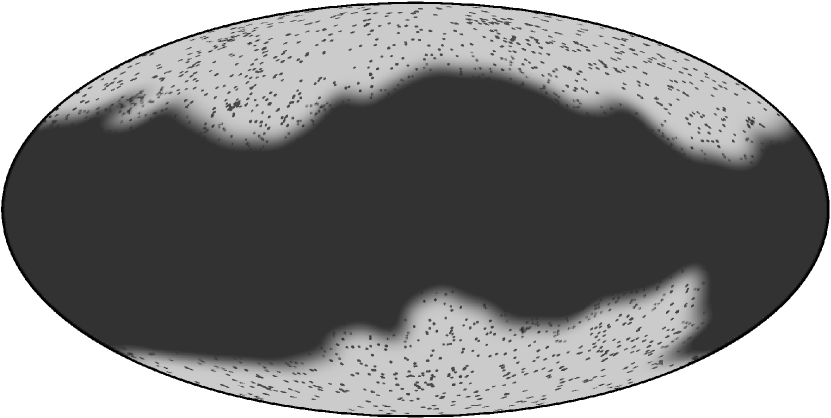
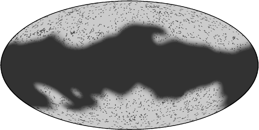
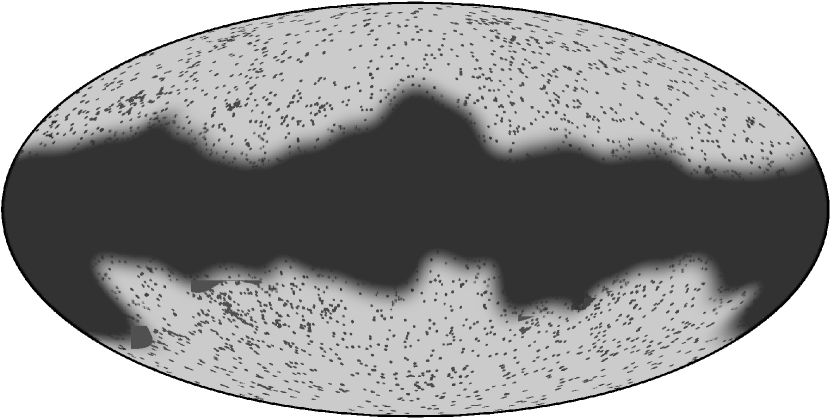
For Planck, we need to estimate the covariance matrices to percent level precision. For temperature spectra, and in the absence of point source holes, this precision can be achieved with sharp, non-apodised Galactic masks (Efstathiou 2004). However, the inclusion of point source holes introduces non-negligible low- power leakage, which in turn can generate errors of a few percent in the covariance matrices. We reduce this leakage by apodising the diffuse Galactic masks (see Appendix B for details). The point source mask is based on the union of the point sources detected between and GHz, and is also apodized. The point source flux cut is not critical, since the amplitudes of the Poisson contributions of unresolved sources are allowed to vary over a wide range in the likelihood analysis. Thus, we do not impose tight priors from source counts and other CMB experiments on the Poisson amplitudes. A set of the combined Galactic and point source masks, referred to as ‘CLx’, where ‘x’ is the percentage of sky retained, are shown in Fig. 2.
3.2 Galactic emission
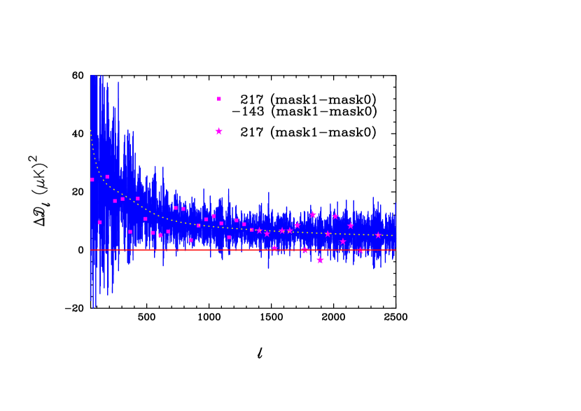
The contamination from diffuse Galactic emission at low to intermediate multipoles can be reduced to low levels compared to CMB anisotropies by a suitable choice of masking. However, even with conservative masking, the remaining Galactic emission at high multipoles is non-negligible compared to other unresolved components, such as the Cosmic Infrared Background (CIB) anisotropies at 143 and 217 GHz. A clear way of demonstrating this is by differencing the power spectra computed with different masks, thereby highlighting the differences between the isotropic and non-isotropic unresolved components. Figure 3 shows (up to ) the 217 GHz power spectrum difference for the mask1 and mask0 masks333 These are the combination of the non-apodised Galactic masks G35 and G22 with the apodised point source mask PSA82., minus the corresponding difference for the GHz frequency channel. Any isotropic contribution to the power spectrum (CMB, unresolved extragalactic sources, etc.) will cancel in such a double difference, leaving a non-isotropic signal of Galactic origin, free of the CMB induced cosmic variance scatter. Above , Fig. 3 shows the mask differenced 217 GHz power spectrum, as the instrumental noise becomes significant at for the 143 GHz channel.
In the same figure, these difference spectra are compared to the unbinned mask-differenced 857 GHz power spectrum, scaled to 217 GHz adopting a multiplicative factor444The scaling coefficient for the 143 GHz spectrum is , derived from the 7-parameter fitting function of Eq. 87. of ; the dotted line shows a smooth fit to the unbinned spectrum. The agreement between this prediction and the actual dust emission at GHz is excellent, and this demonstrates conclusively the existence of a small-scale dust emission component with an amplitude of at 217 GHz if mask1 is used.
For cosmological parameter analysis this small-scale dust component must be taken into account, and several approaches may be considered:
-
1.
Fit to a template shape, e.g., as shown by the dotted line in Fig. 3.
-
2.
Reduce the amplitude by further masking of the sky.
-
3.
Attempt a component separation by using higher frequencies.
The main disadvantage of the third approach is a potential signal-to-noise penalty, depending on which frequencies are used, as well as confusion with other unresolved foregrounds. This is particularly problematic with regards to the CIB, which has a spectrum very similar to that of Galactic dust. In the following we therefore adopt the two former solutions.
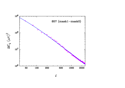
It is important to understand the nature of the small scale dust emission, and, as far as possible, to disentangle this emission from the CIB contribution at the HFI cosmological frequencies. We use the GHz power spectrum for this purpose, noting that the dust emission at 857 GHz is so intense that this particular map provides an effectively noise-free dust emission map. In Fig. 4 we again show the 857 GHz mask power spectrum difference, but this time plotted on a log-log scale. The solid line shows the corresponding best-fit model defined by
| (9) |
with , , , and . At high multipoles this fit asymptotically approaches , which is compatible with previous knowledge about diffuse Galactic emission, i.e., a power-law behaviour with an index close to extending to high multipoles (see e.g., Miville-Deschênes et al. 2007).
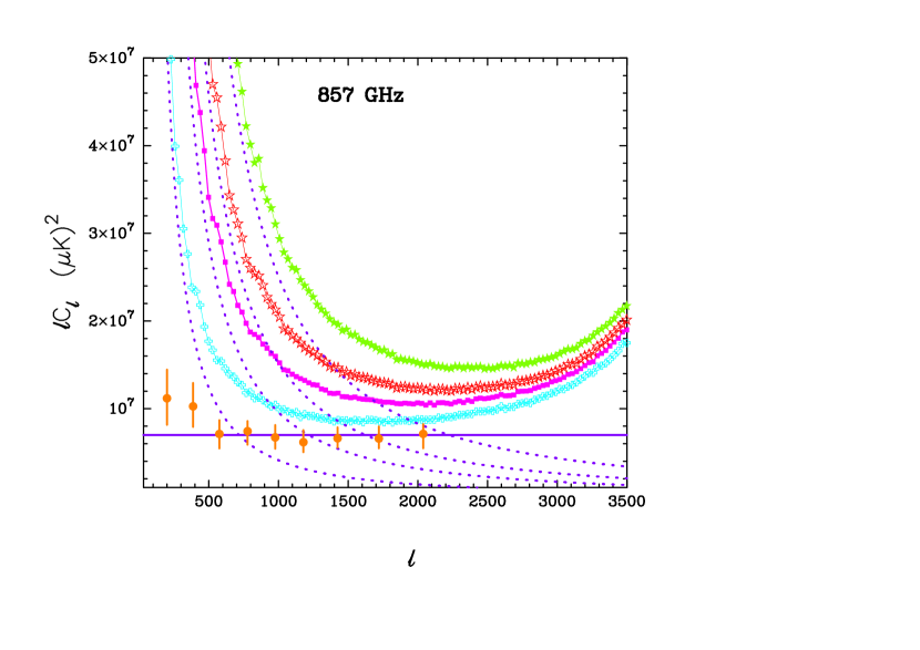
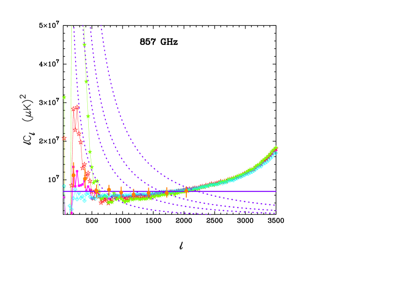
The upper panel in Fig. 5 shows the 857 GHz spectra for the four Galactic masks (G22, G35, G45 through to G56) with the point-source mask applied. They are compared to the 857 GHz CIB power spectrum from Planck Collaboration et al. (2011c), which for can be described approximately as . The best fit models of Eq. 9 are also shown, fitted to , where we expect diffuse emission to be dominant. The lower panel of Fig. 5 shows the same power spectra after subtracting the best-fit dust model. After subtracting the Galactic dust component, the recovered power spectra are consistent with the CIB measured in Planck Collaboration et al. (2011c) for all masks. The excess at high multipoles may be due to a combination of aliasing of large scale power through the point source masks at , Galactic point sources, and uncertainties in the 857 GHz beams.
The model explains by construction the ‘double-difference’ plot shown in Fig. 3. Specifically, this emission is consistent with a cirrus-like power spectrum, , extrapolated to high multipoles. Furthermore, the results of Fig. 5 demonstrate that over a wide area of sky, we can understand the 857 GHz power spectrum in terms of a ‘universal’ cirrus spectrum together with an isotropic CIB component. These results provide strong evidence that an extragalactic CIB component dominates over the diffuse Galactic emission at multipoles over the full range of HFI frequencies outside the CL31 mask.
We take a different approach for the Galactic dust correction with the Plik likelihood. Rather than correcting the empirical spectra during a pre-processing step, the Plik likelihood implements an explicit one-parameter model that describes the dust contribution to the cross-spectrum between detectors and ,
| (10) |
Here
| (11) |
where the dust amplitude, , is measured in units of , is the reference frequency for map , is a reference frequency which is taken to be 143 GHz, is the emission law of a blackbody with temperature , and the dust color-correction terms, , are computed by integrating the dust spectrum within the spectral band of each detector (set). We fix the frequency and angular scaling parameters to , and .
3.3 Poisson power from unresolved point sources
Unresolved galaxies contribute both shot noise and clustered power to the Planck maps. The Poisson contribution leads to a scale independent tem, . We model this power with a single amplitude parameter for each auto-spectrum (, , and ) and a cross correlation coefficient for each cross spectrum (). These quantities are not of primary interest for cosmological results, so to avoid modelling error we do not separate the power into that sourced by “dusty" or “radio" galaxies (i.e., with increasing or decreasing brightness with frequency, respectively) as is done in the analysis of the ACT and SPT power spectra (Dunkley et al. 2011; Reichardt et al. 2012; Dunkley et al. 2013). We also make no assumptions about their coherence between frequencies.
The Poisson power can be related to the flux density via
| (12) |
where we have explicitly introduced the Planck flux cut . Since Planck utilizes a constant signal-to-noise cut, and the Planck noise varies significantly across the sky, this flux cut has a spatial dependence. Although this does not alter the shape of the Poisson term, extra care must be taken when comparing results555One must also account for the fact that these numbers correspond to the amplitude for a suitably averaged spectral band, which is approximately that of the map, and is described in detail in Planck Collaboration IX (2013). with models of . In Sect. 7.3, we explore the consistency between the Poisson power recovered from the Planck power spectrum analysis and predictions from source count measurements.
3.4 Clustered power from unresolved point sources
Unresolved galaxies also contribute power because they trace large-scale structures. The mean flux from the radio galaxies is much smaller than that from the dusty galaxies, so only the dusty galaxies contribute a significant clustering term (Millea et al. 2012). The CIB clustering has been studied extensively, starting with Bond et al. (1986, 1991). Further theoretical investigation (Scott & White 1999; Haiman & Knox 2000) was stimulated by the detection of the infrared background in the COBE data (Puget et al. 1996; Fixsen et al. 1998), and the detection of bright “sub-millimeter” galaxies in SCUBA data (Hughes et al. 1998). Subsequently, the clustering has been detected at 160 microns (Lagache et al. 2007), at 250, 350 and 500 microns by the Balloon-borne Large Aperture Submillimeter Telescope (BLAST, Viero et al. 2009; Hajian et al. 2012) and at 217 GHz by SPT and ACT (Hall et al. 2010; Dunkley et al. 2011). Recent Planck measurements of the Cosmic Infrared Background (Planck Collaboration et al. 2011c) have extended the measurements at 217 GHz, 353 GHz, and 545 GHz to larger scales, and recent Herschel measurements (Amblard et al. 2011) have improved on the BLAST measurements and extended them to smaller angular scales.
Rather than attempt to establish a physical model of the CIB, we adopt in this analysis a phenomenological model that captures the CIB uncertainties for both Planck and high- experiments. Our baseline CIB model is a power-law spectrum with a free spectral index, with an amplitude at each frequency, and , and a cross-correlation between frequencies, . We assume that the CIB clustering power at 100 GHz is negligible.
3.5 Unresolved Sunyaev-Zeldovich effects
Based on analysis of ACT and SPT data, the thermal Sunyaev-Zeldovich (tSZ) contribution is expected to contribute approximately at 100 GHz and at 143 GHz (Reichardt et al. 2012; Dunkley et al. 2013; Sievers et al. 2013). The kinetic Sunyaev-Zeldovich (kSZ) effect is expected to have a similar, or smaller, contribution, with . In addition, theoretical arguments (Reichardt et al. 2012; Addison et al. 2012c) suggest that there should be a tSZ x CIB correlation that should contribute about the same order of magnitude as the kSZ term at 143 GHz.
For Planck, all of these SZ contributions are small in comparison to other unresolved foregrounds and are therefore poorly constrained by Planck data alone. Nevertheless, to eliminate biases in cosmological parameters (Millea et al. 2012; Zahn et al. 2005), we model their contributions, with appropriate constraints from higher resolution CMB experiments, using three templates.
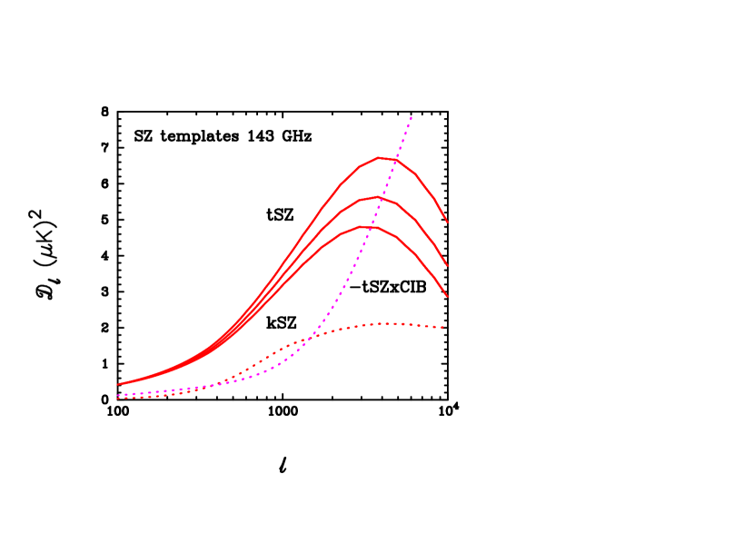
First, for the thermal SZ effect we adopt the family of templates described by Efstathiou & Migliaccio (2012). These are based on the Komatsu & Seljak (2002) model, but use the ‘universal’ X-ray electron pressure profile, , of Arnaud et al. (2010) extrapolated to high redshift via
| (13) |
Here, describes departures from self-similar evolution, and a value of , which is adopted as the default for parameter estimation purposes, provides a good match to the results from recent hydrodynamical numerical simulations incorporating feedback processes (Battaglia et al. 2010, 2012). Figure 6 shows the tSZ templates for three values of ; the template shape is not particularly sensitive to . We treat the (dimensionless) normalization of the tSZ template at GHz as an adjustable parameter,
| (14) |
This parameter fixes the amplitude at GHz via the frequency dependence of the tSZ effect,
| (15) |
We neglect the tSZ at 217 GHz.
Second, for the kinetic SZ effect we adopt the template described by Trac et al. (2011), and as in Eq. 14 we treat the dimensionless amplitude of the template, , as a free parameter,
| (16) |
Third and finally, for the cross-correlation between the thermal SZ component and the CIB we adopt the template described by Addison et al. (2012b). In this case, the amplitude is parameterised in terms of a single correlation coefficient,
| (17) |
These templates are plotted in Fig. 6, normalized to and with using a fiducial CIB amplitude. Note that with these parameters, the tSZ x CIB cross-spectrum approximately cancels the kSZ spectrum at GHz.
As seen in Fig. 6, the SZ contributions are at the level of a few , which, although small, must be taken into account to assess inter-frequency residuals. However, one can see that these templates have similar shapes at multipoles , and therefore they cannot be disentangled using Planck data alone. On the other hand, higher resolution experiments can break this degeneracy, and as shown in Planck Collaboration XVI (2013), the combination of Planck, ACT, and SPT, better constrains the amplitude of the thermal SZ effect. The ACT and SPT data at GHz can be fitted to high (sub-K2) accuracy without kSZ and tSZ x CIB templates, yet we expect a kSZ contribution of at least the amplitude shown in Fig. 6, and larger if we account for patchy reionization (see, e.g., Knox 2003, and references therein) and references therein). This implies a cancellation of the kSZ and tSZ x CIB contributions at GHz (Addison et al. 2012c), as discussed in greater detail in Planck Collaboration XVI (2013).
4 Combined cross-spectra and consistency checks
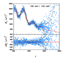
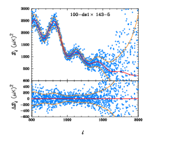
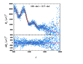
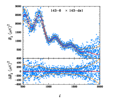


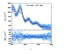
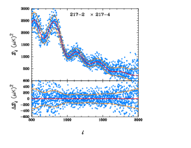
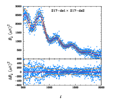
The large number of cross spectra in a detector-by-detector power spectrum analysis allows for a number of internal consistency checks of the data. Within a frequency band, we expect to see exactly the same sky signals (primordial CMB, Galactic, and extra-galactic foregrounds), and so any intra-frequency residuals will reflect instrumental systematics, for example beam errors, ‘gain’ fluctuations, and band-pass mismatch. In contrast, inter-frequency residuals are harder to analyse because the sky signals vary with frequency. An accurate model of the unresolved foregrounds is therefore required to assess inter-frequency residuals. Furthermore, as we will show below, the scatter caused by chance CMB–foreground cross-correlations can dominate the inter-frequency residuals. For a precision experiment such as Planck, where the power spectra are expected to be signal dominated over a wide multipole range, intra- and inter-frequency residuals provide a powerful way of assessing possible systematic errors. It is essential that contributions of systematic errors to both types of residual are small enough that they have negligible impact on cosmological parameter analysis.
Figure 7 shows a selection of temperature cross-spectra and estimates of the analytic covariance matrices, together with the best-fit cosmological model described in Sect. 5. Unresolved foregrounds have been subtracted using the best-fit foreground parameters of the model described in Sect. 3. The scatter varies substantially between cross-spectra, reflecting differences in the instrument noise and effective resolution of different detector combinations. The analytic error model summarized in Appendix A.2 is indicated, modified by the non-white noise correction. This model provides an excellent description of the scatter seen in the data, over the full multipole range shown in plots, with an accuracy of a few percent or better.
4.1 Intra-frequency residuals
In this section we analyse the intra-frequency residuals at and GHz. There are cross-spectra at GHz and cross-spectra at GHz666there is only one cross-spectrum at GHz. At each frequency, we solve for multiplicative (‘effective’ calibration) coefficients, , that minimise
| (18) |
where
| (19) |
subject to the constraint that (where corresponds to detector 5 at GHz and detector 1 at GHz). Note that the power spectra in Eq. 18 and 19 are corrected for beam transfer functions. To minimise the possible impact of beam errors and noise, we restrict the sum in Eq. 18 to the multipole range where the spectra are signal dominated. Numerical values for the calibration coefficients are given in Table 3, using mask CL31. The calibration factors are insensitive to the choice of mask or multipole range.
| map map 143-5 1.0000 217-1 1.0000 143-6 0.9988 217-2 0.9992 143-7 0.9980 217-3 0.9981 - - 217-4 0.9985 143-ds1 0.9990 217-ds1 0.9982 143-ds2 0.9994 217-ds2 0.9975 |
The results of Table 3 show that effective calibration factors of 0.2 % are quite typical for HFI maps, in the GHz frequency range. These recalibrations are of the order of magnitude of the statistical errors of the calibrations on dipole (see Planck Collaboration VIII 2013, Table 2). Note that the data are corrected for individual bolometer time transfer functions (TTFs; Planck Collaboration VII 2013). For each detector, the TTF model is tuned to minimise survey differences and by construction normalised to unity at the spin frequency of the satellite ( Hz) to preserve the dipole calibration. The consistency of intra-frequency power spectrum residuals therefore provides a test of the consistency of the TTFs in addition to the beam transfer functions.
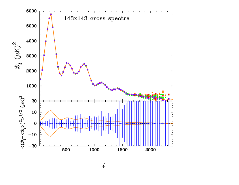
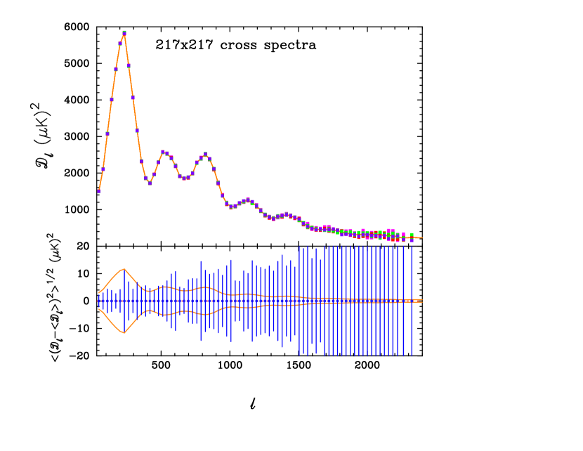
Figure 8 shows the remarkable consistency of the power spectra at each frequency. The upper panels show the spectra corrected for the beam and effective calibration, together with the mean cross spectra. The lower panels show the dispersion around the mean. In the signal dominated regime the cross spectra show an RMS dispersion of a few (in bands of width ), i.e., the band-averaged spectra are consistent to an accuracy of 0.1–0.2 %. This excess scatter has negligible impact on cosmological parameter analysis.
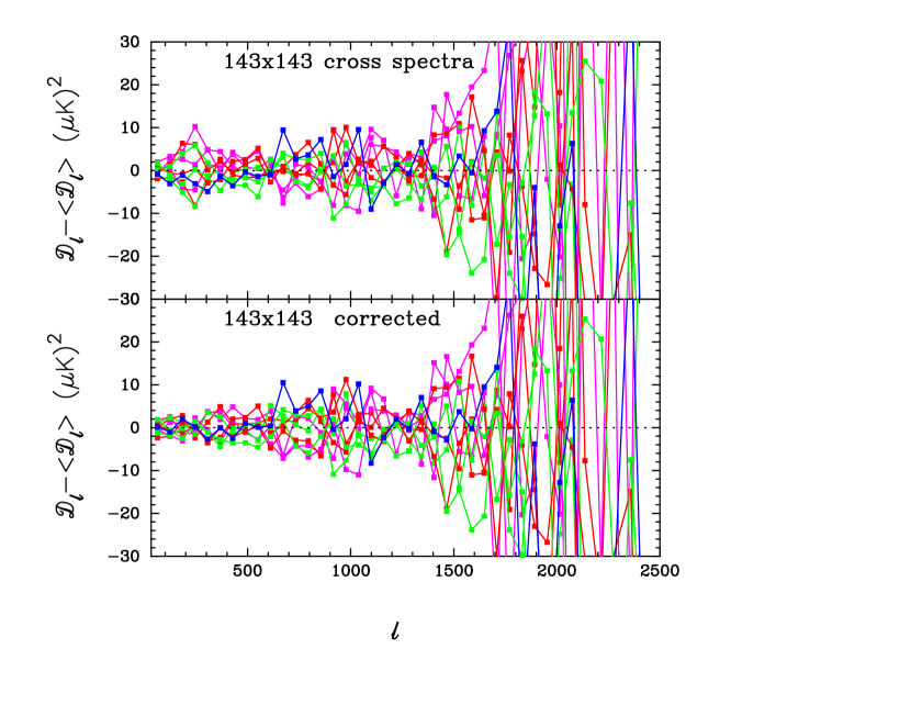
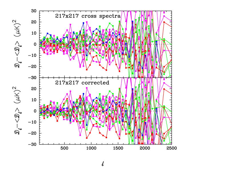
The residuals of the cross spectra in band averages of width are shown in Fig. 9, before and after correction for the effective intra-frequency calibrations. The reduction in scatter after correction is evident at , and the residual scatter is consistent with instrument noise and beam errors. At 217 GHz, beam errors dominate over noise at multipoles . There is no evidence that the excess scatter is caused by a small number of ‘anomalous’ detectors.
4.2 Inter-frequency residuals
The results of the previous section show that the intra-frequency cross-spectra between detector/detector sets are consistent to within a few at multipoles . In a likelihood analysis, there is therefore little loss of information in compressing the power spectra for each distinct frequency combination, as opposed to retaining the spectra for each map pair. This compression greatly reduces the size of the data vector and its covariance matrix, and speeds up the likelihood computation at high multipoles. In this section we inter-compare the residuals of these compressed power spectra.
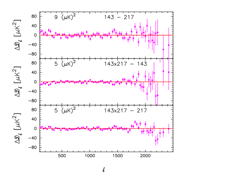
One might naïvely expect that with accurate foreground modelling, the inter-frequency residuals in the signal dominated regime should be reduced to levels comparable to those seen in the intra-frequency comparisons described in the previous section. This is incorrect. Figure 10 shows power spectrum differences between the cosmologically significant spectra for Planck at high multipoles (, , ). In this figure, which is independent of the cosmological model, the best-fit unresolved foreground model has been subtracted from each spectrum, and relative calibration factors have been applied. Residual beam, calibration and unresolved foreground errors would show up in this figure as large-scale smooth residuals.
In fact, we see small-scale residuals at multipoles which are considerably larger than expected from instrumental noise. This excess scatter arises from chance CMB–foreground cross-correlations. Even if the foreground contamination is much smaller than the CMB, chance cross-correlations can produce scatter in the inter-frequency power spectra that is large in the signal dominated regime. We demonstrate in Appendix C that the observed scatter can be predicted quantitatively.
At high enough multipoles, instrument noise, beam errors, and errors in foreground modelling dominate the inter-frequency residuals. A complete analysis of inter-frequency residuals therefore requires the full likelihood machinery and MCMC analysis to determine foreground, beam and calibration parameters. We will therefore revisit the inter-frequency residuals in the following sections.
5 Reference results of the high- likelihood
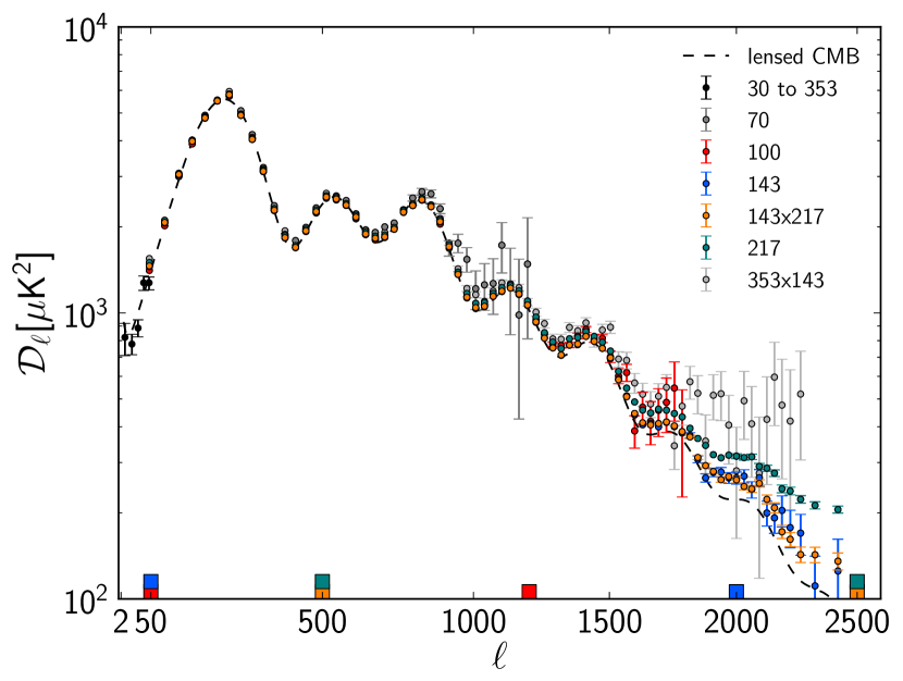
In this section we study the high- Planck likelihood, and present the power spectrum and parameters derived from the baseline likelihood for the basic six-parameter CDM model. In order to break the well-known degeneracy between the optical depth, , and the scalar index of scalar perturbations, , we adopt a Gaussian prior on (inspired from WMAP7 data, i.e., , see Komatsu et al. 2011) instead of the low- likelihood at . We return to the global Planck results after introducing the low- likelihood.
We choose separate masks for each frequency map to minimise Galactic foreground emission. First, since the HFI data are signal-dominated at , and diffuse Galactic emission is low at GHz outside the CL49 mask, there is little to be gained from analyzing the dustier GHz with the same region; it contains no new information about the primordial CMB. At higher multipoles, , we use the CL31 mask, optimizing the sky coverage while ensuring a low amplitude of small-scale Galactic emission relative to the isotropic unresolved foregrounds and the primordial CMB. In addition, we tune the multipole range for each frequency to mitigate Galactic foreground contamination and beam errors.
The choices of masks and angular ranges used in the high- likelihood are summarised in Table 4, together with basic statistics with respect to the minimal CDM model per cross-spectrum and combined. The 100 GHz cross-spectrum is computed over the largest sky fraction, a total of 49% of the sky, and measures the largest scales. On the other hand, it has lowest resolution, and it is therefore only used for . The 143 GHz cross-spectrum has higher resolution, and is used for . Finally, the 217 GHz cross-spectrum has the highest resolution, but also the most Galactic dust contamination, and is therefore evaluated from only 31% of the sky, but including an angular range of .
| Spectrum Multipole range Mask PTE . 50 – 1200 CL49 1.01 0.40 . 50 – 2000 CL31 0.96 0.84 . 500 – 2500 CL31 1.04 0.10 . 500 – 2500 CL31 0.96 0.90 Combined. 50 – 2500 CL31/49 1.04 0.08 |
Given these masks and angular ranges, we compute the angular power spectra and covariance matrices, and construct the CamSpec likelihood. The angular power spectra for each frequency combination are shown in Fig. 11, and compared to spectra derived from the 70 GHz and 353 GHz Planck maps.
| Parameter Prior range Baseline Definition . … Baryon density today . … Cold dark matter density today . … approximation to (used in CosmoMC) . … Thomson scattering optical depth due to reionization . 0 Curvature parameter today with . BBN Fraction of baryonic mass in helium . … Scalar spectrum power-law index () . … Log power of the primordial curvature perturbations () . … Dark energy density divided by the critical density today Age . … Age of the Universe today (in Gyr) . … Matter density (inc. massive neutrinos) today divided by the critical density . … Redshift at which Universe is half reionized . [20,100] … Current expansion rate in |
| Parameter. Prior range Likelihood Definition . C Contribution of Poisson point-source power to for Planck (in ) . P . C As for but at GHz . P . C As for but at GHz . P . C,P Point-source correlation coefficient for Planck between and GHz . C,P Contribution of CIB power to at the Planck CMB frequency for GHz (in ) . C As for but for GHz . P . C,P CIB correlation coefficient between and GHz . C Spectral index of the CIB angular power spectrum () . P . C,P Contribution of tSZ to at GHz (in ) . C,P Contribution of kSZ to (in ) . C,P Correlation coefficient between the CIB and tSZ (see text) . P Amplitude of Galactic dust power (in ) . C Relative power spectrum calibration for Planck between GHz and GHz . . C Relative power spectrum calibration for Planck between GHz and GHz . . C Amplitude of the th beam eigenmode (–5) for the th cross-spectrum (–4) . P Amplitude of the calibration eigenmode for the th detector (set) (–13) . P Amplitude of the th beam eigenmode (–5) for the th detector(set) (–13) |
We use the likelihood to estimate six CDM cosmological parameters, together with a set of 14 nuisance parameters (11 foreground parameters, two relative calibration parameters, and one beam error parameter777The calibration parameters and are relative to the GHzcross-spectrum, whose calibration is held fixed. Only the first beam error eigenmode of the GHz cross-spectrum is explored, all other eigenmodes being internally marginalised over, described in Sect. 3. Tables 5 and 6 summarize these parameters and the associated priors888We use the approximation to the acoustic scale (the ratio of the comoving size of the horizon at the time of recombination, , to the angular diameter distance at which we observe the fluctuations, ) which was introduced by Hu & Sugiyama (1996). is commonly used, e.g., in CosmoMC, to speed up calculations; see also Kosowsky et al. (2002) for further details. . Apart from the beam eigenmode amplitude and calibration factors, we adopt uniform priors. To map out the corresponding posterior distributions we use the methods described in Planck Collaboration XVI (2013), and the resulting marginal distributions are shown in Fig. 12. Note that on the parameters , and we are using larger prior ranges as compared to Planck Collaboration XVI (2013).
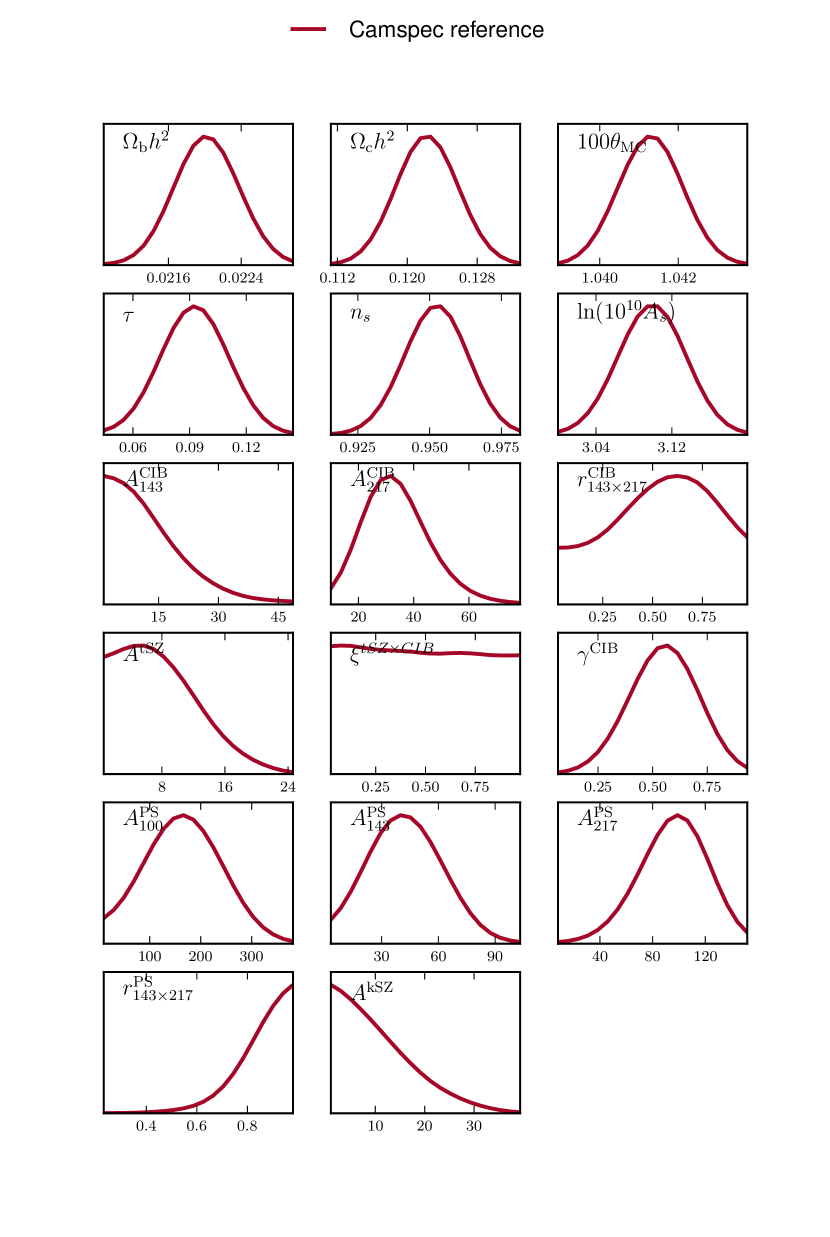
Figure 12 shows the strong constraining power of the Planck data, but also highlights some of the deficiencies of a ‘Planck -alone’ analysis. The thermal SZ amplitude provides a good example; the distribution is broad, and the ‘best fit’ value is excluded by the ACT and SPT high resolution CMB experiments (Reichardt et al. 2012). For the CIB amplitudes, the upper bound on e.g., is significantly weaker than the ACT and SPT constraints. To accurately estimate the foreground parameters at the level, we need to supplement the Planck power spectra with temperature data from ACT and SPT, as described in Planck Collaboration XVI (2013). The fiducial model and foreground parameters used in the CamSpec likelihood are therefore derived from a joint Planck+ACT+SPT analysis and is not based on the parameters listed in Table 8. In the rest of this section, we will use the parameters of Table 8 to discuss inter-frequency residuals.
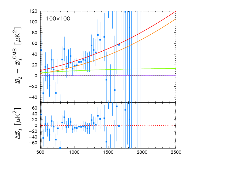
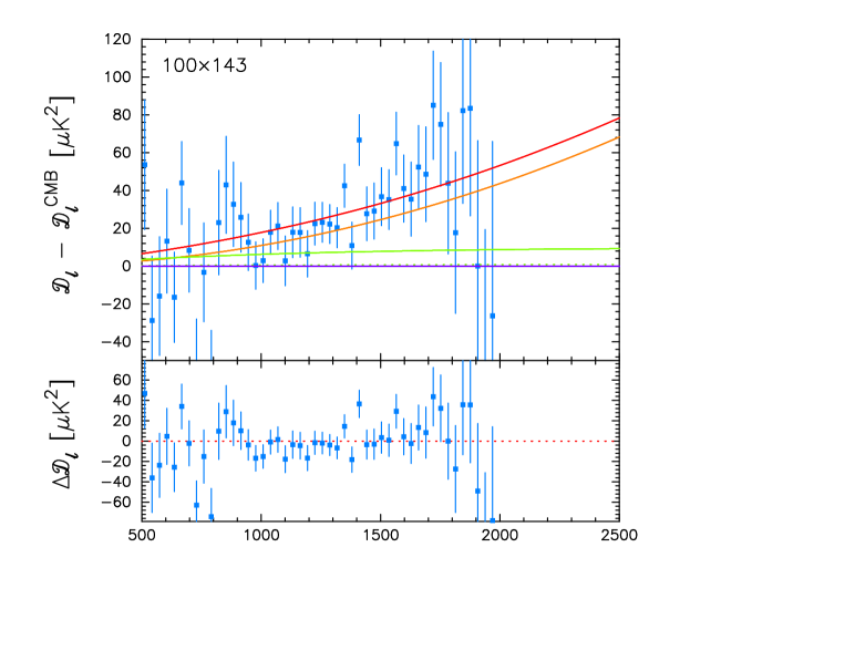
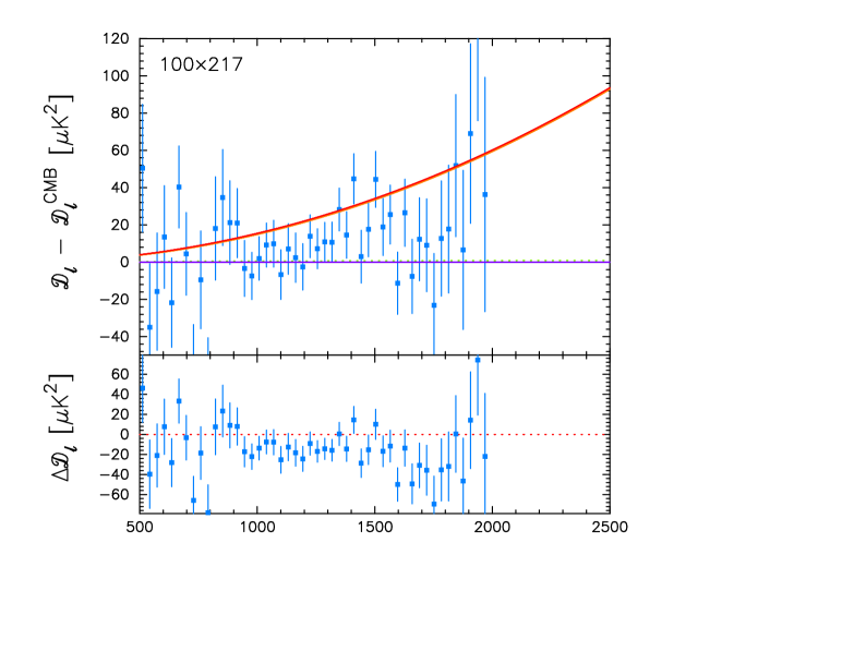
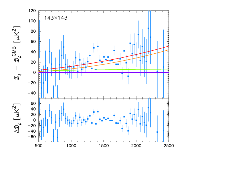
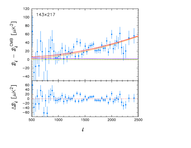
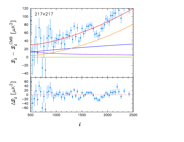
Figure 13 shows the foreground residuals and total residuals after removing the best-fit foreground model for all spectra (including the and spectra, which are not used in the CamSpec likelihood). The first point to note here is that Planck has a limited ability to disentangle foregrounds. While the Planck data constrain the Poisson point source amplitudes at each frequency, as well as the CIB amplitude at GHz (which dominates over the Poisson point source amplitude over much of the multipole range), they have only marginal sensitivity to the tSZ amplitude in the spectrum, though the thermal SZ is strongly degenerate with the Poisson point source amplitude. The remaining foreground parameters are highly degenerate. For Planck alone, these minor foreground contributions combine to absorb inter-frequency residuals.
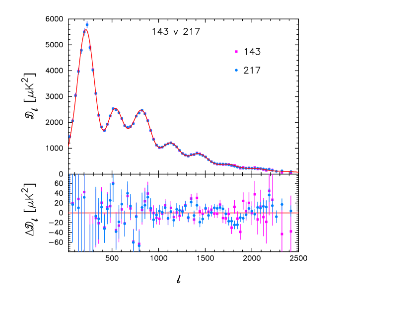
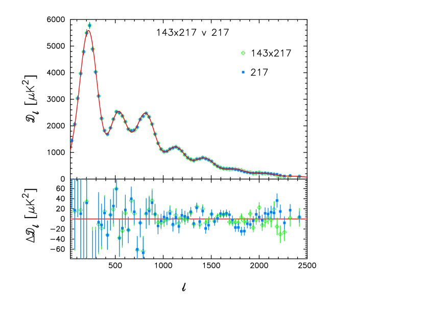
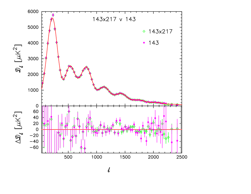
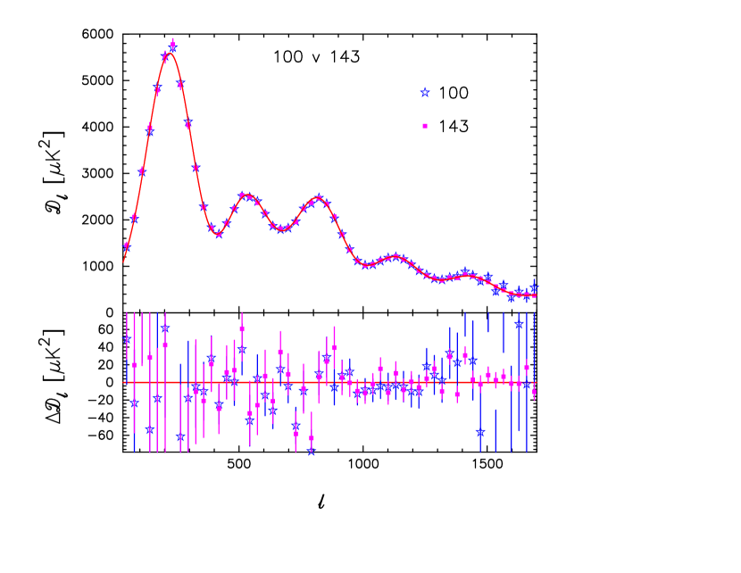
Pairs of spectra are compared in Fig. 14, averaged over bands of width below and wider bands above 2000. (The error bars show the diagonals of the covariance matrices of these averages, but it is important to note that the points are highly correlated even with bin widths as large as these.) This comparison shows that each of the spectra used in the CamSpec likelihood is consistent with the best-fit theoretical spectrum to high accuracy. In fact, each spectrum can be used to form a likelihood, and each gives a reduced close to unity (see Table 4). Thus, the six parameter CDM model provides an excellent fit to the Planck high- power spectra at all frequencies between 100 and 217 GHz.
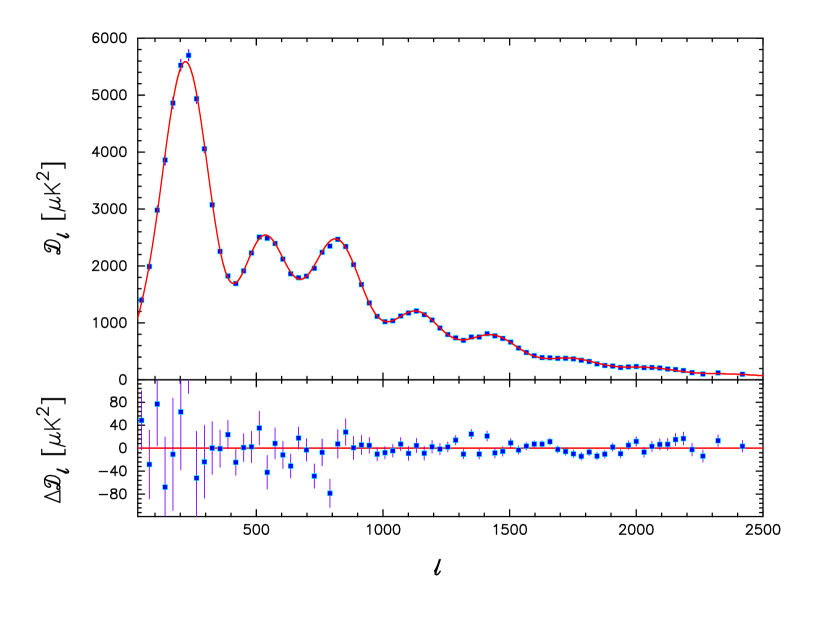
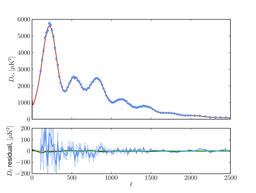
Figure 15 shows our maximum likelihood primary CMB spectrum, together with the best-fit theoretical spectrum. The residuals with respect to the model are shown in the lower panel. The error bars are computed from the diagonal components of the band-averaged covariance matrix. The binning scheme is the same as in Fig. 14.
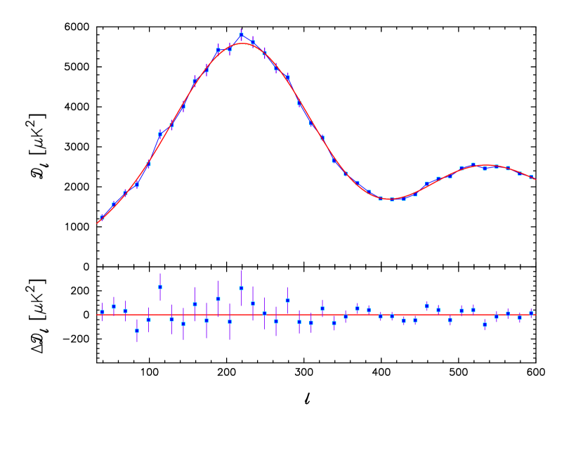
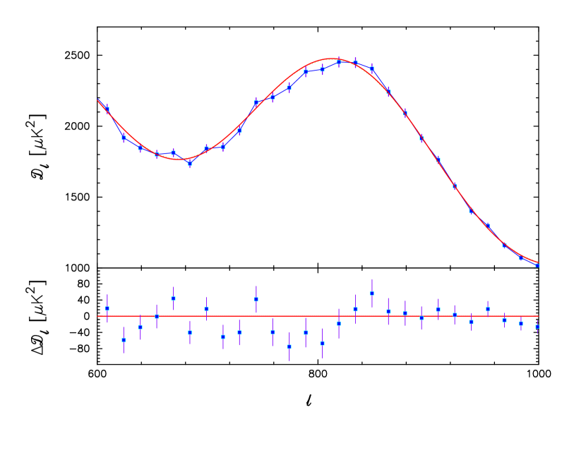
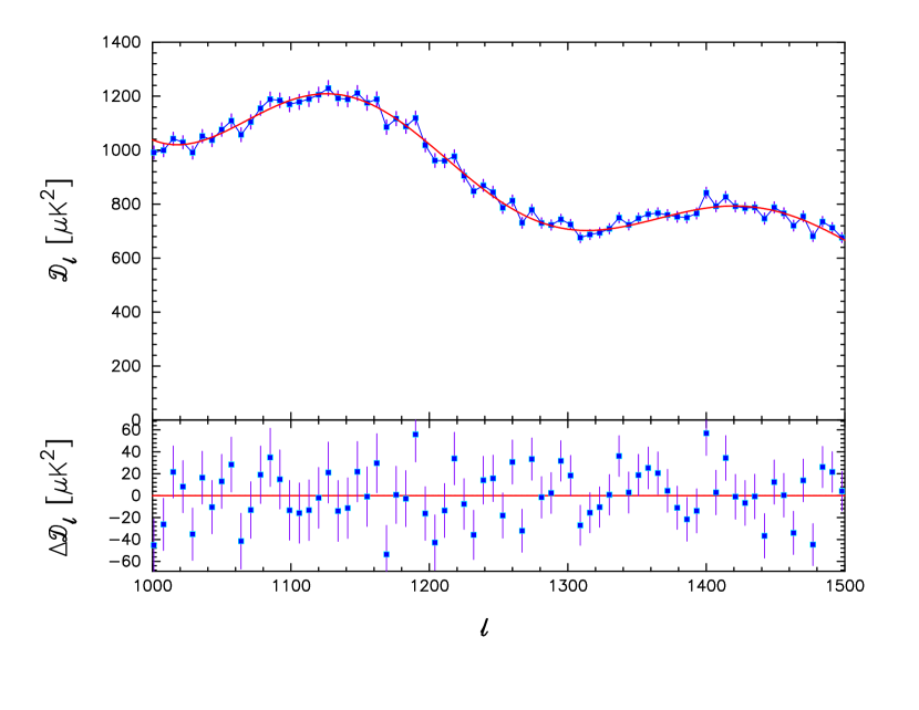
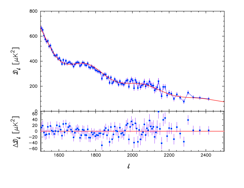
Finally, in Fig. 16 we zoom in on this spectrum in four multipole ranges using finer binning. The correlated fluctuations seen in this figure are mask-induced, and perfectly compatible with the six parameter CDM model. Features such as the ‘bite’ missing from the third peak at and the oscillatory features in the range are in excellent agreement with what we expect from our covariance matrices and from simulations; see Appendix A.4 for a few specific examples.
6 Accuracy assessment of the high- likelihoods
In this section we compare the power spectra and likelihoods derived using our two independent methods, and test the likelihoods using full Planck simulations.
6.1 Comparison of the Plik and CamSpec likelihoods
To allow a consistent comparison between the CamSpec and Plik likelihoods, we use the same frequency cross-spectra for both codes in the following, i.e., we discard the and GHz frequency combinations from the default Plik likelihood. To achieve this, we modify the Plik likelihood to use the fiducial Gaussian approximation instead of the Kullback divergence. On the other hand, while we use the same multipole coverage, , and only one mask (CL39) for all cross-spectra for Plik, we still use multipole ranges and masks as defined in Table 4 for CamSpec. In addition, we perform one Plik analysis with the CL49 mask, which matches the CamSpec mask at GHz.
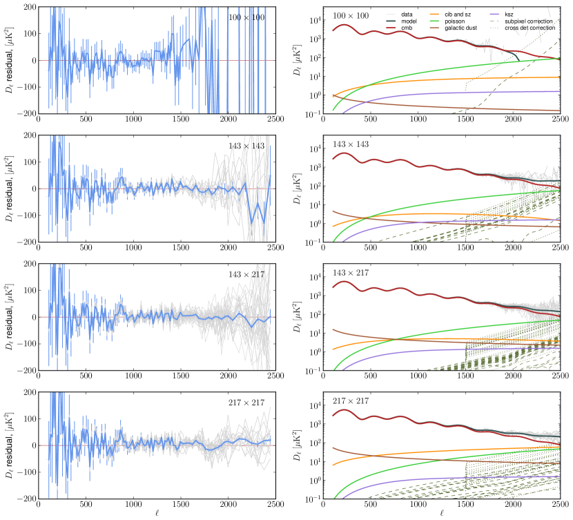
The left column of Fig. 17 shows the differences between the Plik power spectra, adopting the above validation settings, and the corresponding best-fit model. The right column shows the total spectra decomposed into cosmological and foreground components. The residuals agree with those in Fig. 13, and do not show any evidence of features, except for some excess power in the GHz spectra at small scales, where foreground modelling has the highest impact. At scales , the residuals are coherent between cross spectra as they are computed with the same Galactic mask, and the residuals are dominated by cosmic variance. At smaller scales () the residuals are dominated by noise and become uncorrelated.
In Fig. 18 we show the CMB power spectrum recovered by Plik estimated by removing the best-fit foreground amplitudes from each cross-spectrum and computing their optimally weighted average, and the corresponding difference with respect to the best-fit CDM model. The large scatter at low multipoles is expected due to cosmic variance. The residual scatter at higher multipoles is at the level, demonstrating the good fit provided by the sum of the CDM and foreground models. These CMB residuals can be compared to the CamSpec inverse-covariance weighted CMB residuals shown in Fig. 15, which are of the same order of magnitude. Thus, the Planck likelihood fit to the CDM model is robust with respect to the detailed shape of the likelihood, as quantified in terms of power spectrum residuals.
The CDM parameter constraints derived from the two likelihoods are shown in Fig. 19, while Fig. 20 shows the foreground parameters. For the cosmological parameters, the agreement between the two likelihoods is excellent: when the CL49 mask is adopted for the Plik likelihood, which is also used by CamSpec at 100 GHz, all parameters agree to in terms of maximum posterior values. We also see that the widths of the distributions are quite similar, with the Plik ones slightly broader than the CamSpec ones. Significantly larger differences are seen for the foreground parameters.
These effects can be understood as follows: we use the CamSpec likelihood with Galactic mask CL49 for the GHz spectra, to minimize the cosmic variance in the low to intermediate multipole range (, taking advantage of the low level of Galactic emission in this channel. At higher multipoles we use the more conservative Galactic mask CL31 for both the and GHz channels, at the price of a higher variance. However, in the specific case of the CDM model considered here, most of the constraints on cosmological parameters come from relatively modest multipoles, , rather than from the damping tail. This explains why when we repeat the Plik analysis, enlarging the sky area from Galactic mask CL39 to CL49, we find parameter distributions in good agreement with those of CamSpec. However, the detailed choice of masks, as well as multipole range cuts, does affect the foreground parameters. This is investigated further in Sect. 7.
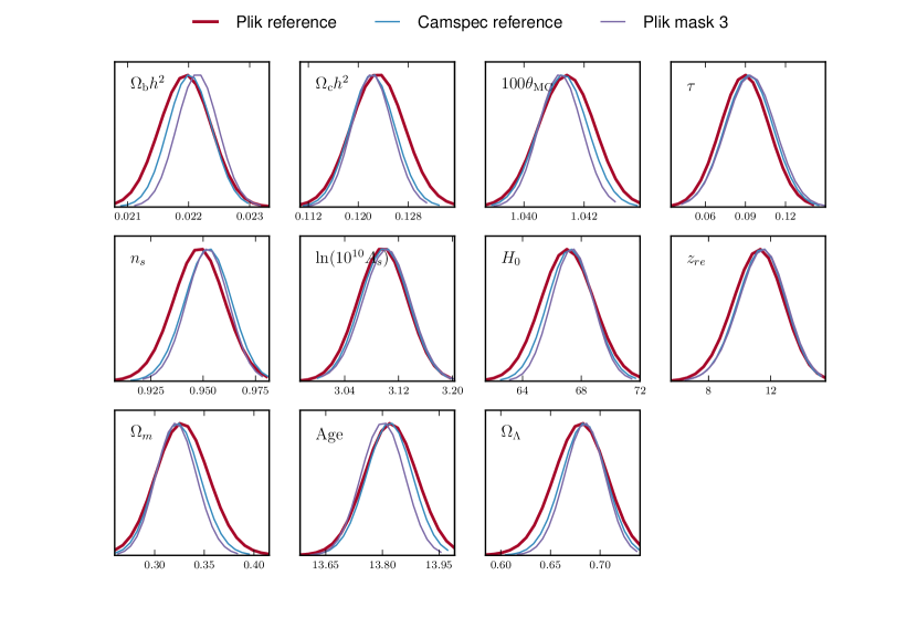
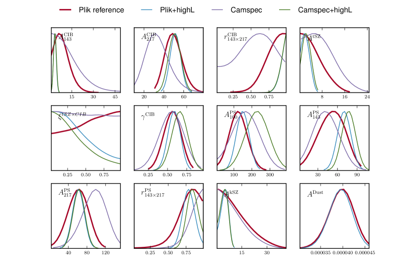
Figure 20 shows the foreground parameters estimated from both Plik and CamSpec. We consider the case for Planck data alone, and with the inclusion of data from ACT and SPT. We also impose, for CamSpec, a Gaussian prior of on the CIB slope parameter, . We find that the upper bounds on the CIB amplitude at GHz, , and on the SZ amplitudes (both thermal and kinetic, and ) are in good agreement using Planck data alone, but we see differences () in the CIB and Poisson amplitudes at GHz (, ) as well as a difference in the CIB correlation coefficient, .
We understand this effect in the following way: CamSpec uses a more limited multipole range and a more conservative mask at GHz than Plik, in order to minimize the Galactic emission in this channel. This enhances the degeneracy between the foreground parameters at 217 GHz, and enhances the sensitivity to possible deviations of the CIB power spectrum from the pure power law assumed here. This is artificially enhanced by normalizing the components at , which is more suitable for high resolution experiments than for Planck. Despite the disagreement of the precise decomposition into the different physical components, the sum of the foreground contributions at GHz in Plik and CamSpec is in good agreement. When ACT and SPT data are added, these problems are largely alleviated, as shown in Fig. 20.
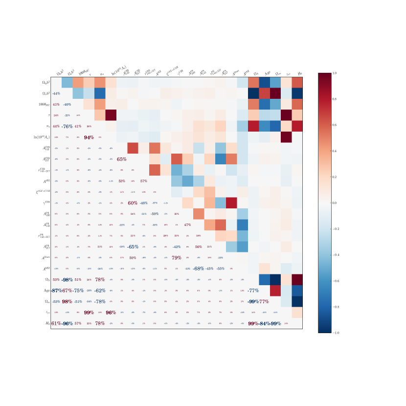
Are these differences important for cosmology? To address this question, we examine the covariance between cosmological and foreground parameters. Figure 21 shows the correlation matrix for all the estimated parameters. The basic CDM parameters have well-known correlations: the scalar spectral index, , is anti-correlated with both the amplitude and the dark matter density , which is itself correlated with the amplitude. Within the foreground parameters, there are strong correlations between the Galactic dust amplitude, the CIB amplitudes, and the SZ amplitude, as well as between point source amplitudes at different frequencies. These correlations result from the conservative foreground model adopted here, where all amplitudes of the CIB and Poisson contributions are left free to vary in each frequency pair; this choice results in small residuals in the fits, at the price of partial degeneracies between the foreground parameters.
Despite this conservative foreground model, there is a small correlation between cosmological and foreground parameters, the strongest effect being a anti-correlation between the kinetic SZ amplitude and the scalar spectral index. The kinetic SZ power spectrum amplitude is positive, so marginalizing over it affects the peak value of despite the fact that is not significantly different from zero. The addition of smaller scale data from ACT and SPT helps to break this degeneracy. In addition, as can be seen in Fig. 20, the posterior distributions of CamSpec and Plik for are in good agreement, showing the stability of the cosmological parameters to the likelihood method.
In Sect. 7, we will further explore the stability of the cosmological and foreground distributions to technical choices made in the likelihood and data selections.
6.2 Comparison to simulations
It is important to demonstrate the precision and accuracy with which cosmological parameters, and foreground parameters to a lesser extent, can be recovered on realistically simulated data. Here we compare the posterior distributions of cosmological and foreground parameters, together with calibration and beam error parameters, inferred using the Plik likelihood, with the input values of a set of simulations, referred to as ‘Full Focal Plane’ (FFP6). The signals in these simulations are based on the ‘Planck Sky Model’ (Delabrouille et al. 2012) which includes a detailed model of the astrophysical emission, both Galactic and extragalactic, at the Planck frequencies. The simulations also reproduce in detail the main instrumental systematic effects of Planck, including correlated timeline noise, instrumental pointing, flags, anisotropic detector beams, and spectral bandpasses. One thousand CMB and noise realisations were generated using the same foreground emission, and a hundred realisations were performed at the level of different detector sets. These simulations are described further in Planck Collaboration ES (2013).
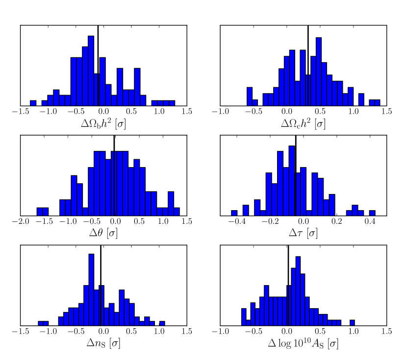
In order to test for any methodological bias, we estimate cosmological parameters from 100 FFP6 simulations using the Plik likelihood. They consist of random realisations of CMB anisotropies and noise, superimposed with a single realisation of a frequency-dependent foreground template. We assume the foreground power spectra to be known exactly, and include their additional power as a constant component in our model. We do not estimate the foreground parameters in this case. This goal of this test is to demonstrate the reliability of our analysis pipeline and explore the effects of the noise and CMB-foreground chance correlations on parameter estimation.
To compare our results to the simulation inputs, we also estimate cosmological parameters from the 100 CMB realisations, without including noise or foregrounds. In the likelihood evaluations we down-weight the high- part of the power spectrum as if there were noise at the level of the noise simulations. A direct comparison of the derived parameters from this CMB-only analysis and the full simulation (that contains noise and foreground emission) allows us to remove the scatter introduced by cosmic variance.
The result of the analysis is shown in Fig. 22, where we plot the distribution of the difference of the mean estimated parameters, between the CMB-only simulation and the noisy CMB simulation with foregrounds, in units of the standard deviation of each individual distribution. An unbiased pipeline will give a difference consistent with zero. Averaged over 100 simulations, only the bias on is statistically significant, but is . An interesting point to note from these histograms is that the distributions are rather wide, mostly around , while by construction, we only studied the effect of noise and CMB-foreground chance correlations in this test.
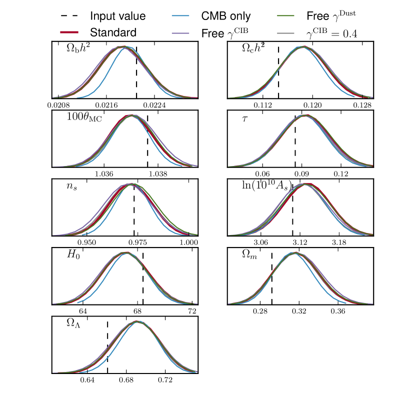
The FFP6 simulations can also be used to assess the sensitivity to foreground modelling errors. In Fig. 23, we compare the posterior marginal distributions of cosmological parameters, estimated with different assumptions about the foreground model. The blue lines, which correspond to the analysis of CMB-only simulations (but accounting for the noise covariance in the likelihood) correspond to the idealised case where the foregrounds play no role, and where the noise-induced variance has been averaged. The red, thick lines show results obtained when marginalising over the parameters of the model of foregrounds that is applied to the Planck data (see Sect. 3), with a fixed value of the CIB spectral index . Purple and grey lines show respectively the effect of leaving free when marginalising, or fixing it to the displaced value of , more than away from the peak posterior. The green lines show the effect of leaving (spectral index of the Galactic dust emission) free in the marginalisation.
The distributions are all in reasonable agreement with the input parameters of the simulation. In addition, we see that varying assumptions on the parameters of the foreground model (red, green, purple, and yellow lines) have negligible impact on the recovered cosmological parameters. Finally, the broadening of the posteriors between the CMB-only exploration and the full case (including noise random realisations and foregrounds) is expected, as the latter includes all the sources of variance, including CMB-foreground and CMB-noise chance correlations.
It is worth noting that the FFP6 foreground simulations, based on extrapolations of existing observations, cannot be described by the simple foreground model used in the likelihood analyses. The upper bounds on biases introduced by a possible mismatch between the simulated foreground templates and the model used in the analysis, inferred from Fig. 22, should be representative of the Planck data analysis. The negligible impact of the various assumptions made on the foreground model parameters of Fig. 23 confirms that the cosmological parameter estimations are robust to details of the foreground model.
7 Consistency checks
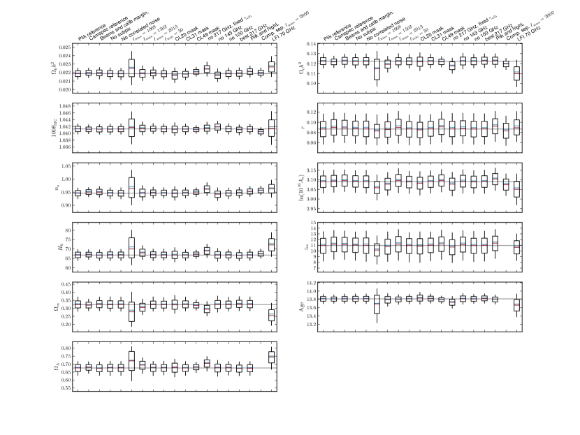
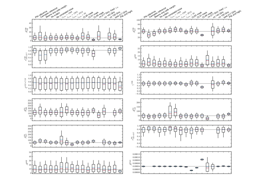
In this section we investigate the stability of the distributions of cosmological and foreground parameters. The technical choices made in constructing the high- likelihood fall into three broad categories. The first category covers internal parameter choices that leave the data selection unchanged. This includes choices such as the binning strategy, marginalizing or not over calibration and beam errors, and the description of the noise model. The second category includes variations in the data selection, such as the multipole range used, and the choice of masks. The final category accounts for variation in the foreground model. We perform a suite of tests to investigate the impact of these choices on parameters. We use the Plik likelihood, and all tests are compared to the baseline Plik spectra. Most of the results can be summarized by ‘whisker plots’ which compare the main properties of the posterior distribution of the cosmological and foreground parameters. More detailed results are reported in Appendix D.1.
In this section we also compare our estimated cosmological parameters to those derived from spectra computed from the LFI 70 GHz channel. We additionally check the consistency of parameters with results obtained using the power spectrum of CMB maps derived by component separation methods (described in Planck Collaboration XII 2013) that use Planck data at all frequencies. This battery of tests demonstrates the stability of the inferred cosmological parameters.
A final test is to compare the predicted polarisation spectrum of the best fitting CDM model with spectra measured from Planck. As discussed in Planck Collaboration I (2013) and Planck Collaboration VI (2013), the Planck polarisation data is not yet used in our cosmological analysis, as further tests must be performed, but the current results increase our confidence in the robustness of the high- temperature likelihood.
7.1 Impact of technical choices for fixed data selection
Here we consider three changes: (1) fixing the inter-frequency calibration and beam errors to the best-fit values, rather than marginalizing, (2) including sub-pixel effects, and (3) including noise correlation between detectors. Figure 24 shows the corresponding impact on parameters.
The effect of fixing the calibration and beam errors is negligible on most cosmological parameters within the six parameter CDM model, with the exception of where we see a shift. There is a bigger effect on the foreground parameters due to their partial degeneracy, and their subdominant contribution to the total power. There is only a small correlation between the cosmological parameters and the calibration coefficients, so marginalizing or fixing their value has little impact on the cosmology.
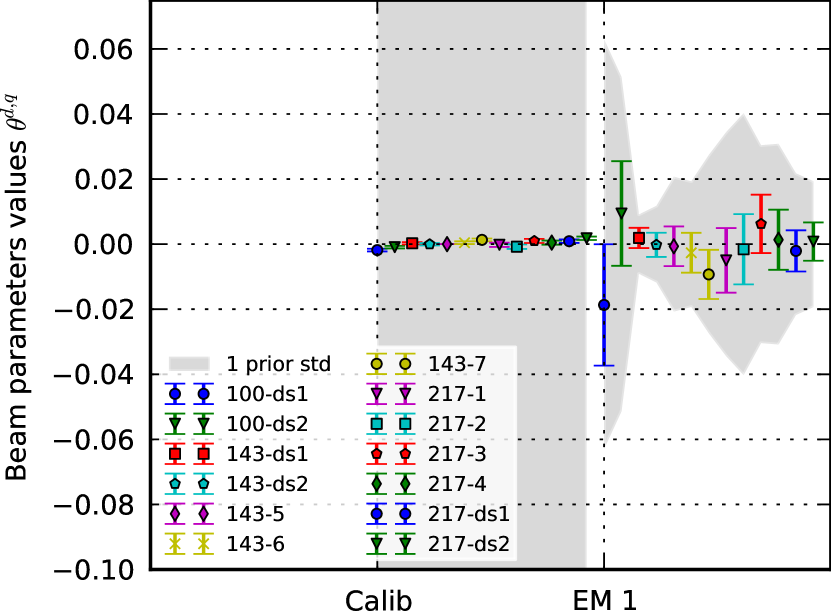
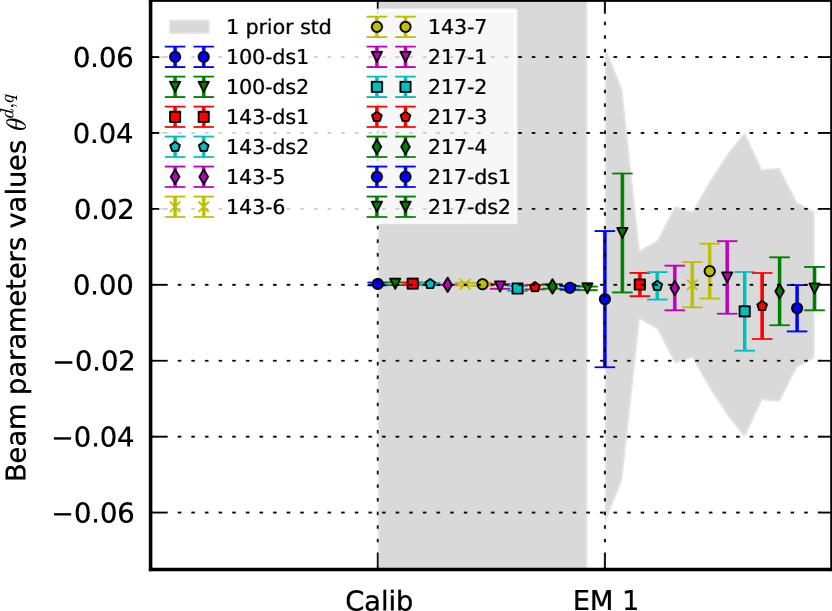
The calibration coefficients are, however, strongly correlated with each other, in particular at GHz, since they are also significantly correlated with e.g., the CIB amplitudes in the and GHz spectra. This is important to keep in mind when comparing the calibration estimates obtained here with those obtained from the CMB dipole in the HFI data processing paper (Planck Collaboration VI 2013). Nevertheless, as can be seen in Fig. 26, the peak posterior values of the relative calibration coefficients are found to differ from at most at the few parts per thousand for all the 13 detectors sets involved, in agreement with the estimates of the calibration accuracy of the maps (Planck Collaboration VI 2013), although a wide flat prior has been applied on these coefficients. The same test applied on simulations with no beam or calibration errors shows how well this test is passed. This confirms that the deviations found at the 0.1% are significantly detected, and it is important to show that these deviations have little impact on the cosmology.
The estimated values of the beam errors do not imply that extra beam corrections are required, with the possible exception of the and 143 -7 detectors (although the corresponding marginal distribution is far from Gaussian). A comparison of the prior and posterior distributions suggests that we have conservatively estimated the uncertainties from the beam determination. We keep this conservative approach in CamSpec, in which we marginalise analytically over all beam eigenmodes except for the dominant 100 GHz mode, , which we sample directly.
As an extended test, we investigate the effect of possible errors in the beam transfer function when the helium abundance is also allowed to vary freely (i.e., without imposing constraints from Big Bang Nucleosynthesis), as it has a larger effect on the small scale spectrum. Varying this parameter leads to a substantial broadening of the posterior distributions for , , and , as can be seen in Fig. 27. We confirm that marginalizing over calibration and beam errors has a small impact on all cosmological parameters, including . On the other hand, it has a somewhat larger impact on some of the foreground parameters (see Appendix D.1).
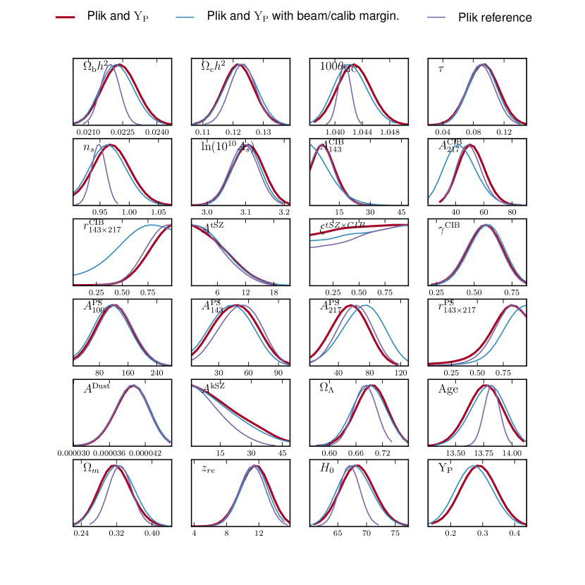
We then investigate the impact of two subdominant effects: the “sub-pixel effect” and the possible presence of a correlation in the noise between detectors or detector sets. The sub-pixel effect has a convolutive effect on the power spectra that is similar to gravitational lensing of the CMB, but is purely a result of the Planck scanning strategy and the map-making procedure (Planck Collaboration VII 2013). The scanning strategy on rings with very low nutation levels results in the centroid of the samples being slightly shifted from the pixel centres; however, the map-making algorithm assigns the mean value of samples in the pixel to the position at the centre of the pixel. This has a non-diagonal effect on the power spectra, but the correction can be computed given the estimated power spectra for a given data selection, and recast into an additive, fixed component of the model covariance matrix.
The possible noise correlation between detectors may appear due to factors such as common residual thermal fluctuations, electronic chain noise, or cosmic ray showers. To build a model of this correlated component, we compute the cross-power spectra between detectors of difference maps that are free of signal. This procedure should capture all correlations on timescales shorter than half a ring’s observation. These estimates are noisy, so we compute an average amplitude of the correlation for .
We find that the impact on parameters of both these effects is negligible, with less then a effect.
7.2 Impact of data selection
Here we consider three changes: (1) varying the angular range used in the likelihood, (2) varying the Galactic mask, and (3) discarding individual frequency channels. These are expected to result in changes in the parameter distributions due to the fact that we are changing the input data.
We first vary the maximum and minimum multipole. Using gives parameter distributions of similar width to those obtained by WMAP. We find that all basic CDM cosmological parameters have converged by , since no parameters are specifically sensitive to the damping tail. The convergence of the posteriors on foreground parameters is, as expected, slower when increasing , as most of them are dominant at small scales. The Galactic dust normalization decreases with due to its correlation with the CIB components. Similarly, changing from to has a negligible effect on cosmological parameters, and mostly affects the determination of the Galactic dust amplitude, which decreases for as it is better measured on large scales; its correlations with the CIB clustered and Poisson contributions explain the slight variations in the corresponding parameters , , and .
We then investigate the impact of varying the Galactic mask, from the most conservative (CL20) to the least conservative (CL49), for fixed multipole range . As expected, the errors decrease as the sky fraction increases. From CL20 to CL39, cosmological and foreground parameters are stable. The foreground parameters change significantly however when we use CL49 for all channels, showing that our foreground model is unable to properly fit the data: the clearest sign of this failure is the unphysically low value of the CIB spectral index (), indicating that our CIB component determination is getting contaminated by a dust-like component with a steeper angular power spectrum than the CIB, but shallower than that of our (single) Galactic dust component. At low Galactic latitudes, the presence of compact Galactic sources leads to a flatter angular power spectrum than that of (high-latitude) diffuse thermal dust, and this likely effects the CIB determination. This justifies the choice made in CamSpec to use a conservative masking strategy (CL31) for the and GHz channels.
Next, we remove one frequency channel at a time. Results change by less than except when removing the GHz channel. This removes a large part of the information and amounts to retaining only 21 cross-spectra out of the 78.
7.3 Testing the Foreground Model
In this section we describe various tests of the foreground model used in the likelihood, checking the validity of our model for the extragalactic sources. Further tests are also reported in Appendix B of Planck Collaboration XVI (2013).
7.3.1 Poisson power from extragalactic sources
Here we check that the Poisson power estimated in the likelihood, which comes from sources below Planck’s detection threshold, is consistent with the level expected given number counts of detected galaxies. Figure 28 shows source counts from Planck (Planck Collaboration Int. VII 2013) at , , and derived from the Planck Early Release Compact Source Catalogue (Planck Collaboration et al. 2011b, a). At and GHz we also show the source counts from SPT as reported in Vieira et al. (2010) at and GHz, and from ACT (Marriage et al. 2011) at GHz. The models of de Zotti et al. (2005) and Tucci et al. (2011) are also shown and are discussed in Planck Collaboration Int. VII (2013).
Planck Collaboration Int. VII (2013) use spectral information to separate the sources into ‘synchrotron’ and ‘dusty’ sources, and show that the counts at 100 – 217 GHz are dominated by synchrotron sources at flux densities above . Vieira et al. (2010) performed a similar separation. The counts at GHz are dominated by synchrotron sources at flux densities , but dusty galaxies contribute roughly equally at GHz at flux densities (Vieira et al. 2010; Hall et al. 2010). The ACT counts have not been separated according to spectral type, but should be dominated by radio sources at these flux densities.
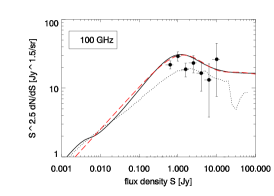
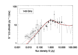
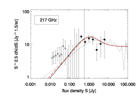
Figure 28 show models fit to the counts using the function
| (20) |
where , , , , , and are free parameters. The best-fit values of these parameters are given in Table 7.
| Parameter 100 GHz 143 GHz 217 GHz . . . . . . |
Given this model, and given the approximate flux cut applied to the Planck maps, the expected contribution of radio sources to the Planck power spectra, at flux densities smaller than , , and mJy at 100, 143, and 217 GHz, are , , and Jy2/sr. The contribution of unresolved infrared galaxies to the power spectra is not negligible. They are expected to dominate at GHz, even if they are subdominant in the Planck counts. Indeed, faint IR galaxies create a “bump” in the distribution, below the detection limit of ACT or SPT. This bump is seen at higher frequencies, e.g., with the Herschel SPIRE instrument (see Planck Collaboration Int. VII 2013, for details).
This bump of infrared galaxies has not been measured at frequencies of GHz and below. However, measurements with the AzTEC telescope at 1.1mm (270 GHz, Scott et al. 2012) can be used to extrapolate the counts down to 217 GHz. This leads to a predicted peak in the number counts () around mJy at a level of , somewhat higher than the values in Hall et al. (2010). The corresponding contribution of infrared galaxies to the power spectrum is estimated in Planck Collaboration XVIII (2011) to be at GHz but with significant uncertainty.
Summing the expected contributions from radio and IR galaxies, we estimate the following values for for Planck: , , and K2 at , , and GHz respectively. These predictions are much less certain at GHz due to the absence of infrared galaxy counts at this frequency.
7.3.2 Clustered power in CIB fluctuations
Here we check the consistency of the estimated clustered power in CIB fluctuations. As already noted, from the CamSpec and Plik likelihoods we find only an upper limit on the clustered CIB power at GHz. With CamSpec we detect clustered power at 217 GHz with K2, and Poisson power with K2. This Poisson power is dominated by the CIB fluctuations. For the Plik likelihood, we have K2 and K2. The sum of the CIB power at 217 GHz, and at pivot scale , is in the range K2.999Note that Planck does not measure directly the CIB power at the pivot scale , hence these extrapolated values are sensitive to possible shape mismatch of the clustered CIB fluctuation power spectra at lower multipoles.
We compare this level to the measurements by the ACT and SPT experiments, which probe higher angular resolution. Fitting a common model to the ACT power spectra from Das et al. (2013), and the SPT spectra from Keisler et al. (2011); Reichardt et al. (2012), the analysis in Dunkley et al. (2013) finds K2 for the CIB clustered component (and K2 for the CIB Poisson component) at effective frequency 219.6 GHz. For SPT, the clustered level is K2 (and Poisson K2), also at an effective frequency of GHz. This is consistent with the SPT analysis in Reichardt et al. (2012). These are estimated assuming and , and that the CIB emission can be modeled with frequency as a modified blackbody, following Addison et al. (2012b).
The total CIB signal seen by Planck, extrapolated to scales, is therefore consistent with the ACT and SPT observations, but given the limited angular range of Planck, the clustered and Poisson part are degenerate. This motivates us to include the ACT and SPT data in many of our cosmological analyses.
When combining Planck, ACT and SPT data together, using the same foreground model (except for Poisson power which depend on the respective flux cuts of the experiments), both CamSpec and Plik give K2, K2, K2, K2, and K2. These estimates of the Poisson power are in good agreement with the predictions given in Sect. 7.3.1 for the and GHz channels. In the latter, radio sources below the Planck flux cuts dominate the Poisson power, which can be reliably estimated from existing source counts measurements.
We also consider modifying our model for the clustered part of the CIB. There have been a wealth of CIB models (e.g., Knox et al. 2001; Amblard & Cooray 2007; Hall et al. 2010; Pénin et al. 2012; Addison et al. 2012a), most assuming that the dust is a biased tracer of the dark matter distribution, but differing in their parametrization of the dust emissivity and its evolution, and their treatment of the dark matter power spectrum. Recent papers (Planck Collaboration et al. 2011c; Addison et al. 2012a) have shown that the addition of Planck CIB measurements, when combined with other small scale probes including SPT, ACT, BLAST, and Herschel, rule out models that assume the underlying dark matter power spectrum is linear.
We therefore test a set of models that try to simultaneously fit the non-linear spectrum with one or more template spectra. We consider fixing the scale dependence to a power law, either or , or extending the power law model to have a running of the index. The model has been used in Shirokoff et al. (2010); Reichardt et al. (2012); Addison et al. (2012b); Dunkley et al. (2013), while the more closely matches the CIB model of Addison et al. (2012a). We find that a simple power law does not fit both the Planck and high- data sufficiently well, but that allowing the additional freedom of a running spectrum opens up the parameter space too much, with little improvement in goodness of fit, motivating our use of the varying model.
We also test a simple model using just a linear theory dark matter power spectrum, assuming that the non-linear power can be absorbed into the Poisson term. This results in an estimate of the Poisson level at GHz that is inconsistent with ACT and SPT, so we do not use this model. For all these models we test the effect on cosmological parameters, using the Hubble constant as a test case, and find the effect on parameters to be small. This is also investigated in Planck Collaboration XVI (2013).
7.4 Consistency of the Planck 70 GHz data
Figure 11 shows individual frequency spectra from 70 to 353 GHz. We only use data from the 100 to 217 GHz channels to form the high- likelihoods, but here we compare cosmological parameters derived from the Planck 70 GHz channel alone. Maps at 70 GHz are easier to characterize than the higher frequency channels in terms of instrumental and foreground properties, but the resolution and sensitivity are lower. The 70 GHz noise properties are in general well described by a simple three parameter model involving and white noise contributions (Planck Collaboration II 2013). The 70 GHz channel also has the least diffuse foreground emission (Planck Collaboration XII 2013), and the extragalactic source contribution is dominated by radio galaxies whose emission is well known at these frequencies (Planck Collaboration XXVIII 2013). We adopt a Galactic plane cut leaving of the sky for the analysis (CS70) to which we add a point source mask optimized for 70 GHz. In Appendix D.2 we describe how cosmological parameters are estimated from the 70 GHz channel, which are summarised in Fig. 24. Accounting for the lower sensitivity and angular resolution at 70 GHz, which translate into a narrower multipole range (), the parameter distributions are consistent with the reference values.
7.5 Consistency with power spectra of CMB maps obtained by component separation methods
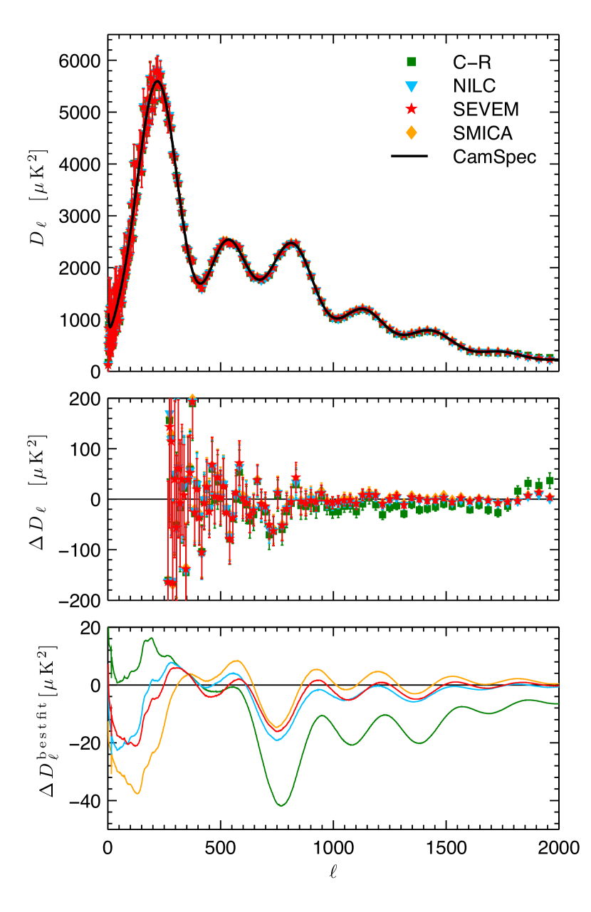
The likelihoods we consider in this paper account for component separation by modeling the multi-frequency data at the power spectrum level, to fully exploit the signal at the smallest scales probed by Planck. We can compare the results to those derived from an alternative approach, measuring the power spectrum of CMB maps estimated from component separation techniques. Here we present results obtained with four CMB maps, derived using methods referred to as Commander-Ruler, SMICA, NILC, and SEVEM, described in detailed in the accompanying paper (Planck Collaboration XII 2013). We compare their angular power spectra and cosmological parameters with those from CamSpec. To estimate the power spectra we use the XFaster method, an approximation to the iterative, maximum likelihood, quadratic band power estimator based on a diagonal approximation to the quadratic Fisher matrix estimator (Rocha et al. 2009, 2010). The noise bias is estimated using difference maps, as described in Planck Collaboration XII (2013). The resulting spectra are shown in Fig. 29, and agree well out to scales , even though the agreement is less striking for the Commander-Ruler small-scale spectrum.
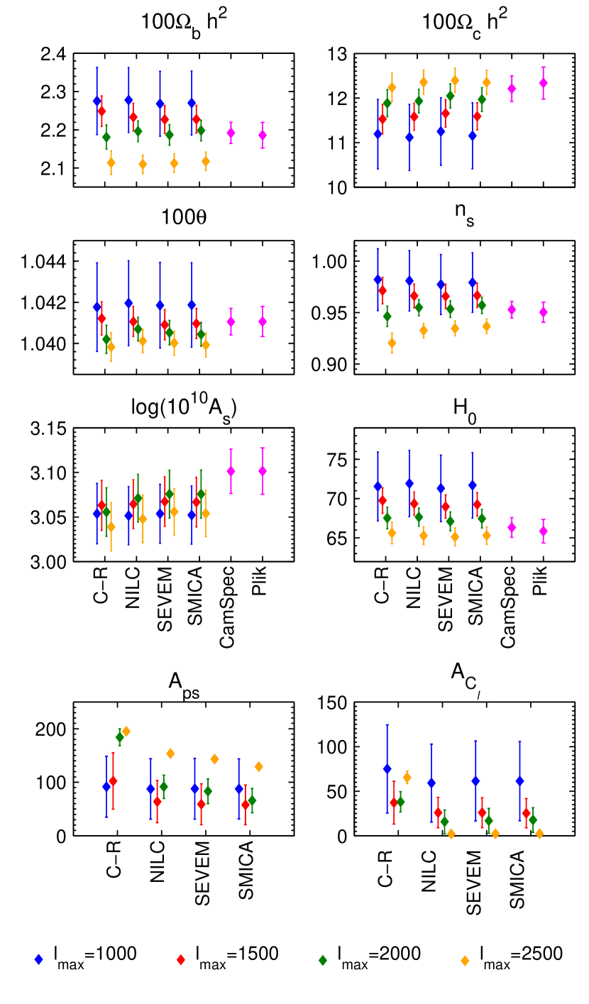
We then estimate cosmological parameters using a Gaussian correlated likelihood derived from these band-powers. To model the residual extragalactic foregrounds, we consider two nuisance parameters: , the amplitude of a Poisson component, and , the amplitude of a clustered component, scaling a term with shape . Figure 30 compares the parameters obtained as a function of for each method, compared to the values from the high- likelihoods. The results are consistent to 1 or better for and . Despite adopting a simple two-parameter model for the extragalactic foregrounds, the likelihood using a CMB map as input data works reasonably well, and may be further exploited with analysis of simulations, improved extragalactic foreground modeling, and the development of an error model.
7.6 Consistency with high- polarisation
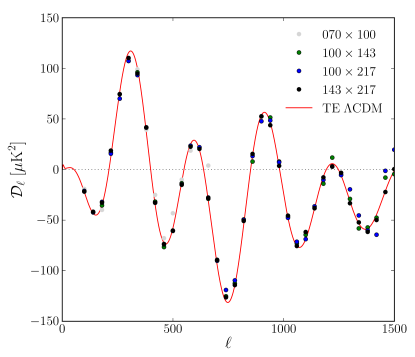
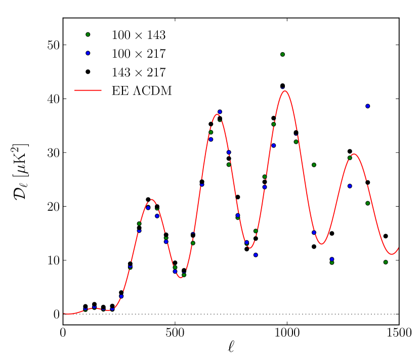
Our final consistency test is illustrated in Fig. 31, showing the polarisation power spectra derived from the Planck data. Both the TE and EE cross-spectra are shown, in bins of width of . These spectra are computed by performing a uniformly weighted average of all detector sets combinations at , , , and GHz. We use the temperature beam window functions for beam deconvolution. For the analysis, we applied CL39 to the temperature maps, and discarded of the polarisation data (i.e., ). Other than masking, no efforts have been made to subtract foreground contributions or take into account instrumental effects such as leakage. Despite the substantial masking applied, we see evidence for residual contributions of non-cosmological origin. Besides demonstrating the potential of Planck to deliver high quality polarisation maps and spectra (with the limitations explained in Planck Collaboration VI 2013), the figure demonstrates the high level of consistency of these polarisation spectra between themselves, and with the prediction from the model fit using just the temperature spectrum shown in Fig. 15.
As discussed in Planck Collaboration VI (2013) and Planck Collaboration II (2013), at present, the HFI and LFI polarisation spectra at low multipoles are affected by systematic errors that cause biases which will need to be accurately modeled or removed for the next Planck release. However, these systematics rapidly become unimportant at higher multipoles. While not yet fit for cosmological parameter analysis, the consistency at the level of a few K of these Planck polarisation spectra adds to our confidence in the analysis of temperature data. It shows that within the CDM framework, the cosmological parameters estimated from Planck temperature data are not strongly affected by the uncertainties in the modelling of unresolved foregrounds.
8 Low- likelihood
At low multipoles (), the distribution of the estimated s is not well approximated by a Gaussian due to the limited degrees of freedom per (e.g., Efstathiou 2004). However, both the CMB signal, , and instrumental noise, , are individually nearly Gaussian distributed at the map level, provided that foreground emission and instrumental systematics effects are negligible (e.g., Planck Collaboration XXIII 2013; Planck Collaboration XXIV 2013), and the actually observed map, , is therefore also nearly Gaussian distributed. Under this assumption, the CMB power spectrum likelihood is given by
| (21) |
where is the number of observed pixels, is the data covariance matrix, and and are the CMB and noise covariance matrices, respectively.
In the general case, the data vector includes both temperature () and linear polarisation (, ) Stokes parameter maps. Pixels exhibiting high foreground contamination are removed by masking, such that the data vector is restricted to the subset of valid pixels, . The corresponding rows and columns are removed from , effectively corresponding to marginalizing over the masked region of the sky. Note that in general, , and the sets of indexes of temperature and polarisation measurements will be different. We assume the same number of pixels in and , although this is not a requirement.
The signal covariance matrix can be written symbolically as
| (22) |
where the signal correlations for the temperature component are explicitly given by
| (23) |
Here are the Legendre polynomials, and is the angle between the centres of pixels and . Similar expressions are available for the polarisation correlations (e.g., Tegmark & de Oliveira-Costa 2001). The effect of the (azimuthally symmetric) instrumental beam, , and pixel window function, , are encoded in .
The main problem with the likelihood expression given in Eq. 21 is its high computational cost. This is determined by the matrix inversion and determinant evaluations, both of which scale as with . In practice, this approach is therefore limited to coarse pixelizations, , which reliably only supports multipoles below . On the other hand, the Gaussian approximation adopted by the high- likelihood is not sufficiently accurate for the stringent requirements of Planck below . In the next section, we therefore describe a faster low- likelihood estimator, based on Gibbs/MCMC sampling, which allows us to exploit the full range up to with low computational cost, while additionally supporting physically motivated foreground marginalization.
Page et al. (2007) pointed out that the temperature and polarisation parts of the likelihood can be separated and evaluated independently, under the assumption of negligible noise in temperature and in the temperature-polarisation cross correlations (i.e., the and blocks of the pixel level noise covariance matrices). Further assuming vanishing primordial modes and correlations, the correlations can be accounted for by redefining the modified and maps as
| (24) | ||||
| (25) |
where are spin weighted spherical harmonics and are the harmonic coefficients of the signal in the temperature map. One can show by direct substitution that these modified and maps are free of temperature correlations. The polarisation likelihood can be then computed independently from the temperature likelihood and, possibly, at lower resolution to save computational expenses. We test this strategy in Sect. 8.2, and adopt it for the current release of the Planck likelihood.
8.1 Low- temperature likelihood
As discussed above, we do not implement the likelihood expression given in Eq. 21 directly, due to its high computational cost and limited flexibility with respect to foreground modelling. Instead, we adopt the Gibbs sampling approach (Eriksen et al. 2004; Jewell et al. 2004; Wandelt et al. 2004), as implemented by the Commander code (Eriksen et al. 2008), which allows both for physically motivated component separation and accurate likelihood estimation. A similar Gibbs sampling method was used to estimate the low- temperature likelihood for WMAP (Dunkley et al. 2009; Larson et al. 2011), although not simultaneously accounting for component separation.
8.1.1 Methodology
We start by generalizing the above data model to include both multi-frequency observations and a set of foreground signal terms,
| (26) |
Here denotes the observed sky map at frequency , and denotes a specific foreground signal component. As above, the CMB field is assumed to be a Gaussian random field with power spectrum , and the noise is assumed Gaussian with covariance . The foreground model can be adjusted as needed for a given data set, and a full description of the model relevant for Planck is presented in Planck Collaboration XII (2013). In short, this consists of a single low-frequency foreground component (i.e., the sum of synchrotron, anomalous microwave emission, and free-free emission), a carbon monoxide (CO) component, and a thermal dust component, in addition to unknown monopole and dipole components at each frequency.
Given this data model, we map out the full posterior distribution, , using a Monte Carlo sampling algorithm called Gibbs sampling. Directly drawing samples from is computationally prohibitive, but this algorithm achieves the same by iteratively sampling from each corresponding conditional distribution,
It is straightforward to show that is a multivariate Gaussian distribution, and is an inverse Gamma distribution. The foreground distribution, , does not have a closed analytic form, but can easily be mapped out numerically (Eriksen et al. 2008). Thus, all three distributions are associated with simple textbook sampling algorithms.
For CMB likelihood estimation, the crucial intermediate product from the above sampling process is the ensemble of CMB sky samples, . Each individual sample corresponds to one possible CMB realization consistent with the observed data. In the absence of sky cuts, foreground contamination and instrumental noise, this map is identical to the true sky. In that case, the likelihood as a function of is determined by cosmic variance alone, and given by an inverse gamma distribution,
| (27) |
Here we have introduced the realization specific power spectrum, , where are the spherical harmonic coefficients of . In the case of realistic data, we need to marginalize over uncertainties due to sky cuts, foregrounds, and instrumental noise. Hence, Eq. 27 is replaced by an average over all possible sampled CMB realizations,
| (28) |
This expression is known as the Blackwell-Rao estimator (Chu et al. 2005), and is guaranteed to converge to the exact likelihood as the number of samples, , increases. Note that the normalization factor in this expression is unknown, but since the likelihood function is only used to compare different models through an effective likelihood ratio, this factor is irrelevant for actual calculations.
8.1.2 Data selection and preprocessing
As described in Planck Collaboration XII (2013), we include Planck frequencies between 30 and 353 GHz in the low- likelihood. Each frequency map is downgraded from its native resolution to a common resolution of 40′, and projected onto an HEALPix grid. Uncorrelated Gaussian regularization noise is added to each frequency channel map, with an RMS proportional to the spatial mean of the instrumental noise of the corresponding channel, , conserving relative signal-to-noise between channels. The regularization noise level at frequency is . The purpose of this is to make the results insensitive to unmodelled features at scales comparable to and beyond the smoothing scale of 40′, in addition to improve the convergence speed of the Gibbs sampler. The resulting signal-to-noise is unity at , and the additional uncertainty due to the regularization noise is less than below , and less than below .
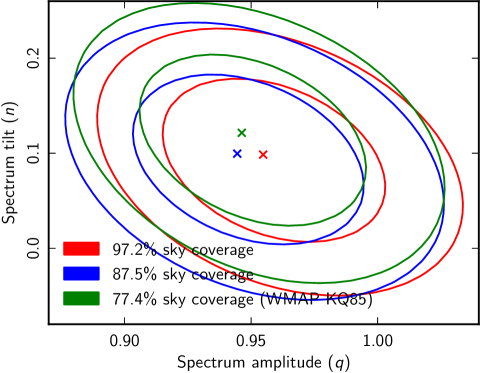
To study the stability of the low- likelihood with respect to sky fraction, we constructed a suite of five different masks, covering between 81 and 100% of the sky, and for completeness we include the WMAP KQ85 mask, covering 75% of the sky, as a sixth case. These low- masks are distinct from those employed for the high- likelihood, and are produced in a preliminary Commander full-sky analysis in which we estimate individual foreground components and residual values per pixel. These maps are thresholded at various levels to produce a useful range of sky fractions.
For each mask, we fit a two-parameter amplitude and tilt power spectrum model of the form , using the low- likelihood between and , where is the best-fit Planck CDM spectrum, and . The resulting distributions are shown in Fig. 32 for three masks, covering 77.4 (A; WMAP KQ85), 87.5 (B) and 97.2% (C) of the sky, respectively. The internal agreement is excellent, with parameters differing by less than between the very aggressive mask A and the conservative mask C. While any of these masks would establish an acceptable likelihood, we adopt Mask B as our fiducial mask for two reasons. On the one hand, the parameter uncertainties obtained with Mask B are only 4% larger than those obtained for the minimal Mask A, indicating that both nearly saturate the cosmic variance limit. On the other hand, analysis of realistic simulations indicate the presence of statistical significant map residuals near the Galactic plane that are accepted by Mask A, but rejected by Mask B (Planck Collaboration XII 2013). The latter therefore represents a good compromise between rejecting foreground residuals and maximizing statistical power.
We include 100 000 Gibbs samples in the likelihood estimator, ensuring excellent convergence characteristics for the Blackwell-Rao estimator for .
8.2 Low- polarisation likelihood
The present Planck data release includes only temperature data. In this release, we therefore supplement the Planck likelihood with the 9-year WMAP polarisation likelihood101010http://lambda.gsfc.nasa.gov derived from the WMAP polarisation maps at 33, 41, and 61 GHz (Ka, Q, and V bands) (Page et al. 2007; Bennett et al. 2012). However, we introduce one modification to this pixel-based likelihood code, replacing the spherical harmonics coefficients of the temperature field, , in Eq. 24 and 25 with those derived from the Planck temperature map derived by Commander, for which the Galactic plane has been replaced with a Gaussian constrained realization.
In Fig. 33, we compare constraints on and as derived with this split likelihood with those obtained through an exact brute-force evaluation of Eq. 21, simultaneously including temperature and polarisation measurements at . The two methods produce almost indistinguishible results.
In Appendix E we assess the robustness of the WMAP polarisation likelihood with respect to dust contamination, by replacing the WMAP polarised dust template with the far more sensitive HFI 353 GHz polarisation map. We find that the optical depth to reionization, , is reduced by about , depending on the template removal method adopted. However, since the Planck polarisation maps are excluded from the current data release, we adopt the WMAP polarisation likelihood without further changes for now, and will return to this topic in the next data release.
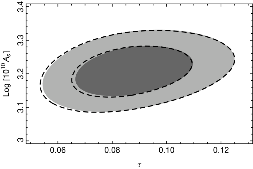
8.3 Low- power spectrum – consistency and robustness
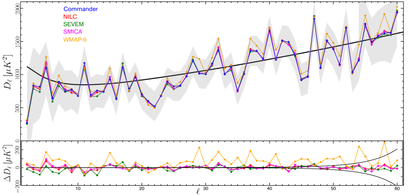
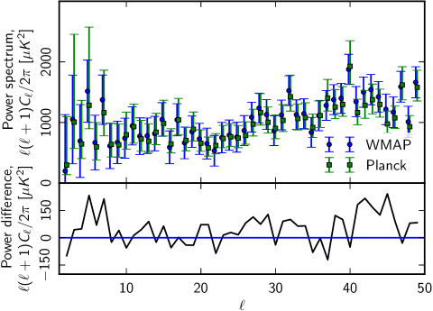
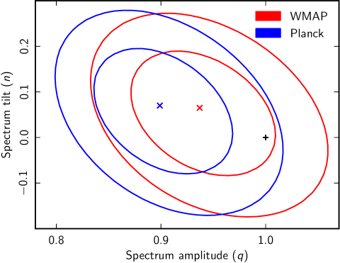
In this section, we present the low- Planck CMB temperature power spectrum derived using the Commander approach described above, and assess its robustness through comparisons with three alternative foreground-cleaned Planck CMB maps (NILC, SEVEM, and SMICA; Planck Collaboration XII 2013), as well as with the 9-year WMAP ILC temperature map (Bennett et al. 2012).
As a first consistency test, we compute the power spectrum from each map using Bolpol (Gruppuso et al. 2009; Molinari et al. 2013), an implementation of the quadratic maximum-likelihood power spectrum estimator (Tegmark 1997). Each map is smoothed to an effective resolution of FWHM, to suppress aliasing from high multipoles (Keskitalo et al. 2010), and repixelized on an HEALPix grid. Gaussian white noise with a variance of 4 K2 is added to each map to regularize the noise covariance matrix.
Here we adopt the U78 common mask, defined in Planck Collaboration XII (2013), to exclude regions of high Galactic emission, leaving 78% of the sky for analysis. We remove the observed monopole and dipole in the mask. The resulting power spectra up to are shown in the top panel of Fig. 34, while the bottom panel shows the power spectrum residuals of each map relative to the Commander map. Note that the same noise realization was added to each map, and the regularization noise therefore contributes little in this plot. For the different internally-derived Planck maps, no residual spectrum exceeds and is typically at . The WMAP spectrum exhibits significantly larger residuals, and are typically of the order of 100 at .
Figure 35 shows the Planck and WMAP temperature power spectra derived directly from the respective likelihood code, while Fig. 36 shows the corresponding constraints on the two-parameter amplitude-tilt model employed in Sect. 8.1.2, including multipoles between and 30. Neglecting the minor differences in the masks adopted by the two codes, these power spectra and parameter constraints are largely dominated by cosmic variance, and one should therefore expect the two distributions to be almost identical. Instead, from Fig. 36 we see that the WMAP low- spectrum is 2.5–3% higher than the Planck spectrum. For a detailed discussion of this discrepancy, including a comparison at higher , see Planck Collaboration XI (2013). Here we only note that the effect is robust with respect to foreground removal and power spectrum evaluation algorithms, and also point out that the effect at low multipoles is too large to be explained by uncertainties in the Planck transfer functions (Planck Collaboration II 2013; Planck Collaboration VII 2013) or calibration (Planck Collaboration V 2013; Planck Collaboration VIII 2013). Also note that the amplitude of the low- spectrum relative to the Planck best-fit model, , derived including the full multipole range between , is somewhat low in Fig. 36, with a best-fit amplitude of . This observation is discussed and quantified in greater detail in Sect. 9.3.
9 The Planck CMB spectrum and likelihood
9.1 Hybridisation of low- and high- likelihoods
The high- and low- likelihoods introduced in Sects. 2 and 8 each describe only a part of the full Planck data set. To estimate cosmological parameters from all the angular scales probed by Planck, they must be combined into a single likelihood function that describes all multipoles from to 2500.
In principle, it is desirable to include as many multipoles as possible in the low- likelihood, since it captures the full non-Gaussian structure of the likelihood. The Gaussian approximation for the likelihood using pseudo-spectra also improves at higher multipole due to the increasing number of degrees of freedom (Efstathiou 2004). For Planck we adopt a transition multipole of , a compromise between obtaining robust convergence properties for the low- likelihood, and ensuring that the Gaussian approximation holds for the high- likelihood (Hamimeche & Lewis 2009).
To combine the likelihoods, we must account for the weak correlations between the low- and high- components. We consider three options:
-
1.
Sharp transition: The low- likelihood ends at ; the high- likelihood starts at ; no correlations are accounted for.
-
2.
Gap: The low- likelihood ends at ; the high- likelihood starts at ; no correlations are accounted for, but the gap is sufficiently wide that any correlations are negligible.
-
3.
Overlap with correction: The low- likelihood ends at ; the high- likelihood starts at ; the double-counting of the overlap region is accounted for by subtracting from the log-likelihood a contribution only including as evaluated by the Commander estimator. Under the assumption that no correlations extend from to , this approach is exact (for further details, see Gjerløw et al. 2013).
We estimate cosmological parameters using all three methods, and find that the posterior means typically vary by . The largest variation is seen including the running of the spectral index of scalar perturbations, in which the posterior mean changes by . Further, all deviations at the 0.1–0.2 level are seen for case 2 above, which excludes data compared to the other two; case 1 and 3 give nearly indistinguishable results. Since case 1 is implementationally simpler, and can be estimated more efficiently (see Sect. 8), we select this method, adopting a sharp transition at .
9.2 The Planck power spectrum and constraints
Using the full Planck likelihood, we now present the final 2013 Planck CMB power spectrum. For this, we fix all nuisance parameters to their maximum-likelihood values. The resulting spectrum is shown in Fig. 37 together with the corresponding best-fit six-parameter model. The agreement between the observations and the model is excellent over most of the multipole range. Only at low s is it possible to see a systematic offset in the form of a slight power deficit; this will be addressed separately in the next section.
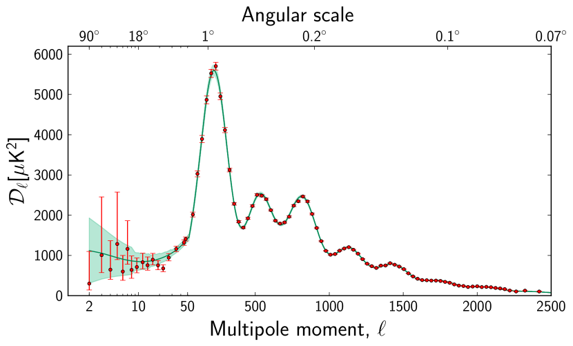
|
|||||||||||||||||||||||||||||||||||||||||||||||||||||||||||||||||||||||||||||||||||||||||||||||||
Table 8 provides a summary of the CDM parameters derived using the methodology described in Planck Collaboration XVI (2013) from the Planck likelihood. Here we use the same prior ranges on all parameters as in Planck Collaboration XVI (2013). These are as in Table 5, except for , , and , which are modified to , , and respectively. Results are given for Planck alone, and in combination with the low- WMAP polarisation likelihood (Planck+WP). For each case, we report both posterior maximum and mean values. Uncertainties denote 68% confidence limits.
A detailed discussion of these results is presented in Planck Collaboration XVI (2013), including an analysis of extended cosmological models, and their compatibility with other astrophysical data sets. The bounds derived from Planck alone are significantly tighter than those from the 9-year WMAP data alone, and comparable or better than those inferred from WMAP combined with SPT and ACT observations. These new constraints provide a precision test of the model. In general, we find good agreement with results derived from other astrophysical data sets, although there are a few exceptions that are in moderate tension with Planck (Planck Collaboration XVI 2013).
Considering each of the six CDM parameters in turn, we first note that Planck constrains the physical baryon density to , which is in remarkable agreement with standard BBN predictions based on a determination of the primordial abundance of deuterium, (Iocco et al. 2009), but with a fractional uncertainty of 1.5,%, three times smaller than the BBN uncertainty. The physical density of dark matter is measured with a fractional uncertainty of 2.6%, providing new constraints on specific dark matter production scenarios. The single most precise parameter, however, is the angular size of the sound horizon at the last-scattering surface, , which is measured with a fractional uncertainty of 0.065 % by Planck, improving on the combined WMAP, ACT, SPT, and SNLS33 constraint by a factor of two.
Next, given that no polarisation data are included in the current data release, it is remarkable that Planck alone constrains the optical depth to reionization, , with a fractional error of 40%. This is made possible by Planck’s high angular resolution and sensitivity, which allows a high signal-to-noise measurement of lensing in the small-scale CMB power spectrum. This in turn breaks the well-known degeneracy between and the amplitude of scalar perturbations, . The fractional uncertainty on from Planck alone is 7 %.
Having sufficient power to measure from small angular scale temperature data, Planck naturally also provides very strong constraints on the spectral index of scalar perturbations, , leading to a fractional uncertainty of 0.97 %. The scale-invariant Harrison-Zeldovich spectrum, , is ruled out at a significance of from the Planck temperature spectrum alone. The analyses presented in Planck Collaboration XVI (2013) and Planck Collaboration XXII (2013) show that the preference for a (red) tilted primordial spectrum remains very strong also within most extensions beyond the minimal model. The implications of this results for inflationary models are discussed in Planck Collaboration XXII (2013).
With our choice of cosmological parameters, the Hubble parameter, , and the fractional density of the cosmological constant, , are derived parameters. They are probed by CMB observations mainly through their impact on , and, to lesser extent, by the impact of on the late-time integrated Sachs-Wolfe effect. Since is accurately measured, a particular combination of and is very well constrained by Planck, although in a model-dependent way; depend on other cosmological parameters, such as the spatial curvature radius, neutrino masses, the number of relativistic degrees of freedom, or a possible dark energy equation of state parameter.
The results reported in Table 8 rely on the assumption of a flat cosmology with three neutrino species, two of which are assumed to massless and one featuring a small mass eV, reflecting the lower bound on neutrino masses imposed by neutrino oscillation experiments. Under these assumptions, Planck finds preferred ranges for and that are lower than previous CMB experiments. For instance, Planck+WP gives , to be compared with for the combined WMAP9+eCMB data set presented by Hinshaw et al. (2012). The underlying cosmology in the two analyses is the same, excepted for the small neutrino mass introduced in our default model. However, if we assume all three neutrino species to be massless, our best-fit and mean values for increase only by . Thus, the tension is clearly driven by the data rather than by theoretical assumptions. Planck Collaboration XVI (2013) shows that our results for and are in very good agreement with Baryon Acoustic Oscillation data, but in moderate tension with other cosmological probes. For instance, our Planck+WP bounds on disagree at the level with direct determinations of the Hubble parameter using cepheids and supernovae (Riess et al. 1998) or quasar time delays (Suyu et al. 2012), as well as with the results of the Carnegie Hubble Program (Freedman et al. 2012). Our bounds on are in a slight tension with the results of the SNLS supernovae collaboration (Conley et al. 2011; Sullivan et al. 2011), although in better agreement with the Union2.1 compilation (Suzuki et al. 2012). Our combined determination of and shows larger tension with recent data based on cosmic shear or cluster count techniques. On the other hand the Planck best-fit model is in good agreement with the halo power spectrum derived from the luminous red galaxy catalogue of the Sloan Digital Sky Survey (Reid et al. 2010), especially when the analysis is restricted to linear scales.
9.3 Significance of the low- tension with CDM models
From the above discussion, it is clear that the CDM framework provides an excellent model for most of the Planck data. However, as noted in Sect. 8.3, and seen in Fig. 37, the low- Planck temperature power spectrum appears to be in some tension with the best-fit Planck CDM model, which for Planck is almost exclusively determined by the small-scale spectrum. In this section we assess the significance and impact of this tension between low and high s using three different statistical tests.
We start by applying a modified Hausman test (Polenta et al. 2005; Planck Collaboration II 2013) to the low- spectra derived from the four foreground-cleaned Planck maps (Planck Collaboration XII 2013) and the 9-year WMAP ILC map, using multipoles up to . This test uses the statistic , where
| (29) | ||||
| (30) |
and and denote the observed and model power spectra, respectively. Intuitively, this statistic measures the relative bias between the observed spectrum and model, measured in units of standard deviations, while taking into account the so-called “look-elsewhere effect” by maximizing over multipole ranges. We use realistic Planck ‘FFP6’ simulations (Planck Collaboration I 2013) to derive the empirical distribution of under the null hypothesis. Figure 38 compares the results obtained from the data with the simulation distribution, and Table 9 lists significances. As measured by this statistic, we see that a negative bias is found in the low- Planck power spectrum relative to the CDM model at the 99% confidence level.
For the WMAP ILC map the significance of the negative bias nominally decreases to 93%. This is consistent with the findings in Sect. 8.3, where it was shown that the WMAP temperature power spectrum is 2.5–3 % higher than the Planck spectrum at low ’s. However, as discussed in Planck Collaboration XI (2013), a similar amplitude difference between the two experiments is also seen at smaller scales. Since the current test compares the observed WMAP data with the best-fit Planck CDM model, the present test is not optimal for assessing internal consistency between low and high s within the WMAP data.
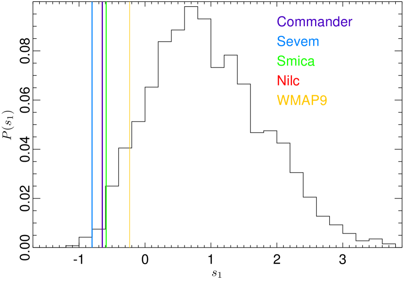
| Data set [%] Commander . -0.647 0.73 NILC . -0.649 0.73 SEVEM . -0.804 0.50 SMICA . -0.589 1.33 WMAP9 ILC. -0.234 7.18 |
Next, to obtain a quantitative measure of the relative power discrepancy between low and high s, we fit the two-parameter amplitude–tilt power spectrum model (see Sect. 8.1.2) to the Planck data using the low- likelihood restricted to various multipole ranges defined by , where is allowed to vary. Thus, this measures the amplitude of the low- spectrum relative to the best-fit Planck CDM spectrum, which is driven by the smaller angular scales. Figure 39 shows the resulting constraints on the power spectrum amplitude, , as a function of , after marginalizing over the tilt, . For comparison, we also show similar constraints derived using the low- WMAP temperature likelihood up to . The best-fit amplitude is for –35, different from unity at a statistical significance of 2– by this measure. The WMAP spectrum shows a consistent behaviour, up to the same overall scaling factor of 2.5–3% between Planck and WMAP discussed above. We have verified that these results are insensitive to the (well-known) low quadrupole moment by excluding from the analysis; the large cosmic variance of this particular mode results in a low overall statistical weight in the fit.
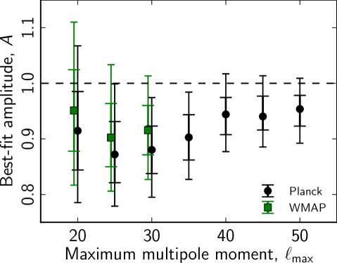
Finally, we assess the impact of the low- power deficit on the CDM model estimated using the Planck likelihood111111We have verified that the following results are insensitive to whether Plik or CamSpec are used for the high- likelihood. (augmented with the WMAP polarisation likelihood). We fit a low- rescaling amplitude, for jointly with the CDM parameters, i.e., for and for . Figure 40 shows the resulting posterior distributions for for (green) and (blue). The purple line shows the same when replacing the Planck low- likelihood with the WMAP low- likelihood (). The corresponding best-fit values are (Planck; ), (Planck; ) and (WMAP; ), respectively. As already noted in Sect. 8.3, these values are too large to be explained by the uncertainties in the Planck transfer functions (Planck Collaboration II 2013; Planck Collaboration VI 2013).
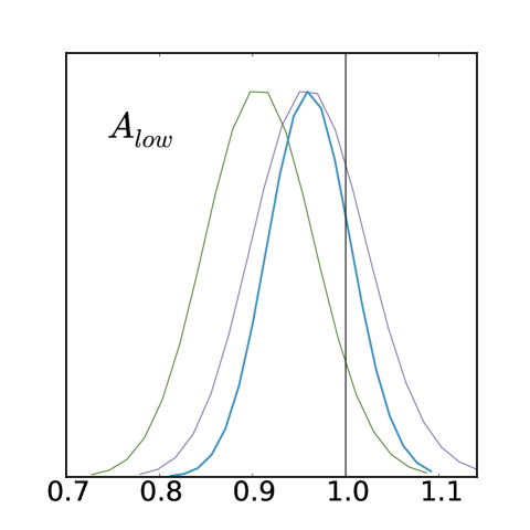
In Fig. 41 we show the posterior distributions for , and after marginalizing over for . (Adopting results in negligible differences for all parameters except ). Shifts of 0.6– are observed compared to the reference model, . We note that , which already has a ‘low’ value (for a detailed discussion, see Planck Collaboration XVI 2013), prefers an even lower value when allowing a rescaling of the low- spectrum. As a final test, we replace the entire low- likelihood, both temperature and polarisation, with a Gaussian prior on the optical depth of reionization, , matching the WMAP measurement (Hinshaw et al. 2012). The resulting posteriors are shown as purple lines in Fig. 41, and agree well with the case including a low- scaling factor, but are, in fact, slightly further away from the reference model. Although not very significant in an absolute sense, these results do indicate that the high- likelihood is challenged in finding models that also fit the low- power spectrum.
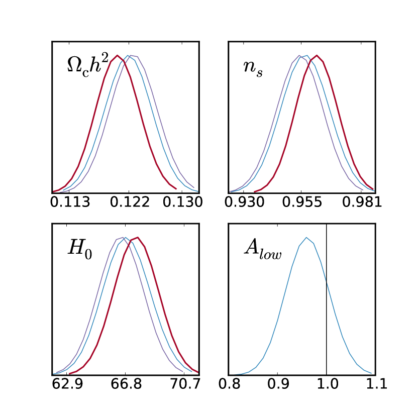
To summarize, we have phenomenologically quantified a tension between the low- CMB power spectrum at and the Planck best-fit model. Its significance varies between 2.5 and depending on the estimator used. The effect is seen in all four Planck foreground-cleaned CMB maps with little variation. It is also present in the 9-year WMAP data, although an overall amplitude difference of 2.5–3 % between the data sets complicate a direct comparison. To make further progress, one would seek to establish a physical model that predicts a low- power deficit compared to high ’s, and that may also predict other observable effects which may be tested with cosmological data. Such a model may be related to the tentative detections of violations of statistical isotropy discussed in Planck Collaboration XXIII (2013), e.g., the low CMB temperature variance, the hemispherical power asymmetry, or the alignment between the quadrupole and octopole moments.
10 Discussion & conclusions
We have presented the Planck likelihood, which provides a detailed and accurate characterisation of the two-point statistics of the CMB temperature field, accounting for all significant sources of uncertainty; statistical, instrumental, and astrophysical. This likelihood function allows us to present an estimate of the CMB temperature power spectrum that spans more than three decades in with unprecedented precision; a spectrum that saturates the cosmic variance limit at all scales , nearly exhausting the information content of the temperature anisotropies, and, in fact, is becoming limited by uncertainties due to astrophysical foreground modelling. This is precisely what was originally promised at the time when Planck was selected by ESA in March 1996.
On large angular scales, , the Planck likelihood is based on a Gibbs sampling approach that allows joint CMB power spectrum and component separation analysis, while accurately marginalizing over a physically motivated foreground model constrained by the 30–353 GHz Planck frequencies. On intermediate and small scales, the Planck likelihood employs a fine-grained set of cross-spectrum combinations among the 100, 143, and 217 GHz detector maps to constrain the high- CMB power spectrum, ensuring that no noise bias can compromise the results, while at the same time allowing for physical foreground modelling in terms of power spectrum templates. This emphasis on physical foreground modelling has made it possible to combine the full power of the Planck data with observations from higher- CMB experiments.
We have validated our results through an extensive suite of consistency and robustness analyses, propagating both instrumental and astrophysical uncertainties to final parameter estimates. Further, we have studied in detail the well-known degeneracies that exist between the foreground and cosmological parameters at high s when only including Planck observations, and shown that they have only a weak impact on cosmological conclusions.
On a more detailed level, we draw the following conclusions:
-
•
The consistency between power spectra measured at different frequencies is remarkable. In the signal-dominated regime for single detectors, at , the cross-spectra show an RMS dispersion of a few in multipole bands of . This confirms the relative calibration of the 100, 143, and 217 GHz detectors to 0.2%.
-
•
The differences, , between the , , and cross-spectra averaged over multipole bands of have a dispersion over of 9, 5, and 5 , respectively, after subtracting the best-fit foreground model. This dispersion is not primarily of instrumental origin, but can be predicted from a model of the chance correlations between foregrounds and CMB fluctuations.
-
•
At high s, the power spectrum of the four foreground-cleaned CMB maps derived through component separation are consistent within their uncertainties. The cosmological parameters derived from these maps are consistent with those estimated by the Planck likelihood for , despite very different foreground models.
-
•
At low s, the power spectrum differences among the four foreground-cleaned CMB maps are below for nearly every single multipole. Residuals with respect to the 9-year WMAP ILC map are slightly larger, typically or more. A detailed comparison between Planck and WMAP reveals a systematic power spectrum amplitude difference at the – level that cannot be accounted for within the Planck instrumental error budget. This is consistent with the findings presented in Planck Collaboration XI (2013).
-
•
Parameters derived from the 70 GHz Planck frequency map are in excellent agreement with the reference results derived using the Planck likelihood; when the latter is limited to , the agreement is even more striking. This confirms the strong internal consistency between the LFI and HFI instruments.
-
•
The best-fit CDM model derived from the Planck likelihood predicts and spectra in exquisite agreement with the measured polarization signature over a broad range of frequencies (70 to 217 GHz) and multipoles (). At 100, 143, and 217 GHz, the instrumental noise in the spectrum is at the level for , and the visible differences between the spectra are dominated by their different levels of foreground contribution, not by systematic effects.
-
•
We report a tension between the Planck best-fit CDM model and the low- spectrum in the form of a power deficit of 5–10% at , with a statistical significance of 2.5–3. Thus, while the minimal model provides an outstanding fit for intermediate and small angular scales, this tension may suggest that the model is incomplete. In this respect, it is worth noting that other, but possibly related, anomalies have been reported in a companion paper studying statistical isotropy in the Planck sky maps at statistically significant levels.
In summary, we find that the majority of the Planck data can be described by a minimal six-parameter model with a very high degree of accuracy. Within this model the statistical uncertainties are dominated by astrophysical foreground modelling by scales of . At lower s, the unprecedented quality of the Planck data is such that the only fundamental limit is that we can only observe one CMB sky. In other words, Planck is cosmic variance dominated at , extragalactic foreground dominated at , and dominated nowhere by instrumental noise or systematic errors.
Using only Planck data, we report a detection of at more than confidence, significantly stronger than the limit derived from WMAP, SPT, ACT, and SNLS3 combined. Complementing the Planck observations with the 9-year WMAP polarization data increases the significance to . The multipole range above is crucial for constraining possible extensions to the minimal CDM model; for a detailed exploration of a wide range of such models, see Planck Collaboration XVI (2013) and Planck Collaboration XXII (2013). There we report some tensions among the CMB damping tail parameters, including , , and . However, none of these indicate significant departures from the framework.
In the near future, we will extend our analysis to produce a cosmic variance limited likelihood and power spectrum reaching to higher multipoles. To some extent, this will be achieved through more sophisticated astrophysical foreground modelling, and by exploiting additional frequency information. However, the two major steps forward will be, first, to include the Planck polarization observations in the likelihood analysis, and, second, to exploit the full data set generated by the two Planck instruments. The amount of HFI data available for analysis is nearly double that which is presented here, and the LFI instrument is still observing at the time of writing.
Acknowledgements.
The development of Planck has been supported by: ESA; CNES and CNRS/INSU-IN2P3-INP (France); ASI, CNR, and INAF (Italy); NASA and DoE (USA); STFC and UKSA (UK); CSIC, MICINN, JA and RES (Spain); Tekes, AoF and CSC (Finland); DLR and MPG (Germany); CSA (Canada); DTU Space (Denmark); SER/SSO (Switzerland); RCN (Norway); SFI (Ireland); FCT/MCTES (Portugal); and PRACE (EU). A description of the Planck Collaboration and a list of its members with the technical or scientific activities they have been involved into, can be found at http://www.rssd.esa.int/index.php?project=PLANCK&page=PlanckCollaboration. We acknowledge the use of the CLASS Boltzmann code (Lesgourgues 2011) and the Monte Python package (Audren et al. 2013) in earlier stages of this work. The likelihood code and some of the validation work was built on the library pmclib from the CosmoPMC package (Kilbinger et al. 2011). This research used resources of the IN2P3 Computer Center (http://cc.in2p3.fr) as well as of the Planck-HFI data processing center infrastructures hosted at the Institut d’Astrophysique de Paris (France) and financially supported by CNES.References
- Addison et al. (2012a) Addison, G. E., Dunkley, J., & Bond, J. R. 2012a, ArXiv e-prints
- Addison et al. (2012b) Addison, G. E., Dunkley, J., Hajian, A., et al. 2012b, ApJ, 752, 120
- Addison et al. (2012c) Addison, G. E., Dunkley, J., & Spergel, D. N. 2012c, MNRAS, 427, 1741
- Amblard & Cooray (2007) Amblard, A. & Cooray, A. 2007, ApJ, 670, 903
- Amblard et al. (2011) Amblard, A., Cooray, A., Serra, P., et al. 2011, Nature, 470, 510
- Arnaud et al. (2010) Arnaud, M., Pratt, G. W., Piffaretti, R., et al. 2010, A&A, 517, A92
- Audren et al. (2013) Audren, B., Lesgourgues, J., Benabed, K., & Prunet, S. 2013, J. Cosmology Astropart. Phys., 2, 1
- Battaglia et al. (2012) Battaglia, N., Bond, J. R., Pfrommer, C., & Sievers, J. L. 2012, ApJ, 758, 75
- Battaglia et al. (2010) Battaglia, N., Bond, J. R., Pfrommer, C., Sievers, J. L., & Sijacki, D. 2010, ApJ, 725, 91
- Bennett et al. (2012) Bennett, C. L., Larson, D., Weiland, J. L., et al. 2012, ArXiv e-prints
- Bond et al. (1986) Bond, J. R., Carr, B. J., & Hogan, C. J. 1986, ApJ, 306, 428
- Bond et al. (1991) Bond, J. R., Carr, B. J., & Hogan, C. J. 1991, ApJ, 367, 420
- Cardoso et al. (2008) Cardoso, J.-F., Le Jeune, M., Delabrouille, J., Betoule, M., & Patanchon, G. 2008, IEEE Journal of Selected Topics in Signal Processing, 2, 735
- Chu et al. (2005) Chu, M., Eriksen, H. K., Knox, L., et al. 2005, Phys. Rev. D, 71, 103002
- Conley et al. (2011) Conley, A., Guy, J., Sullivan, M., et al. 2011, ApJS, 192, 1
- Das et al. (2013) Das, S., Louis, T., Nolta, M. R., et al. 2013, ArXiv e-prints
- Das et al. (2011) Das, S., Marriage, T. A., Ade, P. A. R., et al. 2011, ApJ, 729, 62
- de Zotti et al. (2005) de Zotti, G., Ricci, R., Mesa, D., et al. 2005, A&A, 431, 893
- Delabrouille et al. (2012) Delabrouille, J., Betoule, M., Melin, J.-B., et al. 2012, ArXiv e-prints
- Dunkley et al. (2013) Dunkley, J., Calabrese, E., Sievers, J., et al. 2013, ArXiv e-prints
- Dunkley et al. (2011) Dunkley, J., Hlozek, R., Sievers, J., et al. 2011, ApJ, 739, 52
- Dunkley et al. (2009) Dunkley, J., Komatsu, E., Nolta, M. R., et al. 2009, ApJS, 180, 306
- Efstathiou (2004) Efstathiou, G. 2004, MNRAS, 349, 603
- Efstathiou (2006) Efstathiou, G. 2006, MNRAS, 370, 343
- Efstathiou & Migliaccio (2012) Efstathiou, G. & Migliaccio, M. 2012, MNRAS, 423, 2492
- Eriksen et al. (2008) Eriksen, H. K., Jewell, J. B., Dickinson, C., et al. 2008, ApJ, 676, 10
- Eriksen et al. (2004) Eriksen, H. K., O’Dwyer, I. J., Jewell, J. B., et al. 2004, ApJS, 155, 227
- Fixsen et al. (1998) Fixsen, D. J., Dwek, E., Mather, J. C., Bennett, C. L., & Shafer, R. A. 1998, ApJ, 508, 123
- Fowler et al. (2010) Fowler, J. W., Acquaviva, V., Ade, P. A. R., et al. 2010, ApJ, 722, 1148
- Freedman et al. (2012) Freedman, W. L., Madore, B. F., Scowcroft, V., et al. 2012, ApJ, 758, 24
- Gjerløw et al. (2013) Gjerløw et al. 2013, to be submitted
- Gruppuso et al. (2009) Gruppuso, A., de Rosa, A., Cabella, P., et al. 2009, MNRAS, 400, 463
- Haiman & Knox (2000) Haiman, Z. & Knox, L. 2000, ApJ, 530, 124
- Hajian et al. (2012) Hajian, A., Viero, M. P., Addison, G., et al. 2012, ApJ, 744, 40
- Hall et al. (2010) Hall, N. R., Keisler, R., Knox, L., et al. 2010, ApJ, 718, 632
- Hamimeche & Lewis (2008) Hamimeche, S. & Lewis, A. 2008, Phys. Rev. D, 77, 103013
- Hamimeche & Lewis (2009) Hamimeche, S. & Lewis, A. 2009, Phys. Rev. D, 79, 083012
- Hinshaw et al. (2012) Hinshaw, G., Larson, D., Komatsu, E., et al. 2012, ArXiv e-prints
- Hivon et al. (2002) Hivon, E., Górski, K. M., Netterfield, C. B., et al. 2002, ApJ, 567, 2
- Hu & Sugiyama (1996) Hu, W. & Sugiyama, N. 1996, ApJ, 471, 542
- Hughes et al. (1998) Hughes, D. H., Serjeant, S., Dunlop, J., et al. 1998, Nature, 394, 241
- Iocco et al. (2009) Iocco, F., Mangano, G., Miele, G., Pisanti, O., & Serpico, P. D. 2009, Phys.Rept., 472, 1
- Jewell et al. (2004) Jewell, J., Levin, S., & Anderson, C. H. 2004, ApJ, 609, 1
- Jones et al. (2006) Jones, W. C., Ade, P. A. R., Bock, J. J., et al. 2006, ApJ, 647, 823
- Keisler et al. (2011) Keisler, R., Reichardt, C. L., Aird, K. A., et al. 2011, ArXiv e-prints
- Keskitalo et al. (2010) Keskitalo, R., Ashdown, M. A. J., Cabella, P., et al. 2010, A&A, 522, A94
- Kilbinger et al. (2011) Kilbinger, M., Benabed, K., Cappe, O., et al. 2011, ArXiv e-prints
- Knox (2003) Knox, L. 2003, New A Rev., 47, 883
- Knox et al. (2001) Knox, L., Cooray, A., Eisenstein, D., & Haiman, Z. 2001, ApJ, 550, 7
- Komatsu & Seljak (2002) Komatsu, E. & Seljak, U. 2002, MNRAS, 336, 1256
- Komatsu et al. (2011) Komatsu, E., Smith, K. M., Dunkley, J., et al. 2011, ApJS, 192, 18
- Kosowsky et al. (2002) Kosowsky, A., Milosavljevic, M., & Jimenez, R. 2002, Phys. Rev. D, 66, 063007
- Lagache et al. (2007) Lagache, G., Bavouzet, N., Fernandez-Conde, N., et al. 2007, ApJ, 665, L89
- Larson et al. (2011) Larson, D., Dunkley, J., Hinshaw, G., et al. 2011, ApJS, 192, 16
- Lesgourgues (2011) Lesgourgues, J. 2011, ArXiv e-prints
- Lewis (2008) Lewis, A. 2008, Phys. Rev. D, 78, 023002
- Marriage et al. (2011) Marriage, T. A., Baptiste Juin, J., Lin, Y.-T., et al. 2011, ApJ, 731, 100
- Millea et al. (2012) Millea, M., Doré, O., Dudley, J., et al. 2012, ApJ, 746, 4
- Miville-Deschênes et al. (2007) Miville-Deschênes, M.-A., Lagache, G., Boulanger, F., & Puget, J.-L. 2007, A&A, 469, 595
- Molinari et al. (2013) Molinari et al. 2013, to be submitted
- Page et al. (2007) Page, L., Hinshaw, G., Komatsu, E., et al. 2007, ApJS, 170, 335
- Pénin et al. (2012) Pénin, A., Doré, O., Lagache, G., & Béthermin, M. 2012, A&A, 537, A137
- Percival & Brown (2006) Percival, W. J. & Brown, M. L. 2006, MNRAS, 372, 1104
- Planck Collaboration et al. (2011a) Planck Collaboration, Ade, P. A. R., Aghanim, N., et al. 2011a, A&A, 536, A13
- Planck Collaboration et al. (2011b) Planck Collaboration, Ade, P. A. R., Aghanim, N., et al. 2011b, A&A, 536, A7
- Planck Collaboration et al. (2011c) Planck Collaboration, Ade, P. A. R., Aghanim, N., et al. 2011c, A&A, 536, A18
- Planck Collaboration ES (2013) Planck Collaboration ES. 2013, The Explanatory Supplement to the Planck 2013 results (ESA)
- Planck Collaboration I (2013) Planck Collaboration I. 2013, In preparation
- Planck Collaboration II (2013) Planck Collaboration II. 2013, In preparation
- Planck Collaboration Int. VII (2013) Planck Collaboration Int. VII. 2013, A&A, 550, A133
- Planck Collaboration IV (2013) Planck Collaboration IV. 2013, In preparation
- Planck Collaboration IX (2013) Planck Collaboration IX. 2013, In preparation
- Planck Collaboration V (2013) Planck Collaboration V. 2013, In preparation
- Planck Collaboration VI (2013) Planck Collaboration VI. 2013, In preparation
- Planck Collaboration VII (2013) Planck Collaboration VII. 2013, In preparation
- Planck Collaboration VIII (2013) Planck Collaboration VIII. 2013, In preparation
- Planck Collaboration XI (2013) Planck Collaboration XI. 2013, In preparation
- Planck Collaboration XII (2013) Planck Collaboration XII. 2013, In preparation
- Planck Collaboration XVI (2013) Planck Collaboration XVI. 2013, In preparation
- Planck Collaboration XVIII (2011) Planck Collaboration XVIII. 2011, A&A, 536, A18
- Planck Collaboration XXII (2013) Planck Collaboration XXII. 2013, In preparation
- Planck Collaboration XXIII (2013) Planck Collaboration XXIII. 2013, In preparation
- Planck Collaboration XXIV (2013) Planck Collaboration XXIV. 2013, In preparation
- Planck Collaboration XXVIII (2013) Planck Collaboration XXVIII. 2013, In preparation
- Polenta et al. (2005) Polenta, G., Marinucci, D., Balbi, A., et al. 2005, J. Cosmology Astropart. Phys., 11, 1
- Puget et al. (1996) Puget, J., Abergel, A., Bernard, J., et al. 1996, A&A, 308, L5+
- Reichardt et al. (2009) Reichardt, C. L., Ade, P. A. R., Bock, J. J., et al. 2009, ApJ, 694, 1200
- Reichardt et al. (2012) Reichardt, C. L., Shaw, L., Zahn, O., et al. 2012, ApJ, 755, 70
- Reid et al. (2010) Reid, B. A. et al. 2010, Mon. Not. Roy. Astron. Soc., 404, 60
- Riess et al. (1998) Riess, A. G., Filippenko, A. V., Challis, P., et al. 1998, AJ, 116, 1009
- Rocha et al. (2009) Rocha, G., Contaldi, C. R., Bond, J. R., & Gorski, K. M. 2009, ArXiv e-prints
- Rocha et al. (2010) Rocha, G., Contaldi, C. R., Colombo, L. P. L., et al. 2010, ArXiv e-prints
- Scott & White (1999) Scott, D. & White, M. 1999, A&A, 346, 1
- Scott et al. (2012) Scott, K. S., Wilson, G. W., Aretxaga, I., et al. 2012, MNRAS, 423, 575
- Shirokoff et al. (2010) Shirokoff, E., Reichardt, C. L., Shaw, L., et al. 2010, ArXiv e-prints
- Sievers et al. (2013) Sievers, J. L., Hlozek, R. A., Nolta, M. R., et al. 2013, ArXiv e-prints
- Spergel et al. (2003) Spergel, D. N., Verde, L., Peiris, H. V., et al. 2003, ApJS, 148, 175
- Story et al. (2012) Story, K. T., Reichardt, C. L., Hou, Z., et al. 2012, ArXiv e-prints
- Sullivan et al. (2011) Sullivan, M., Guy, J., Conley, A., et al. 2011, ApJ, 737, 102
- Suyu et al. (2012) Suyu, S. H., Auger, M. W., Hilbert, S., et al. 2012, ArXiv e-prints
- Suzuki et al. (2012) Suzuki, N., Rubin, D., Lidman, C., et al. 2012, ApJ, 746, 85
- Tegmark (1997) Tegmark, M. 1997, Phys. Rev. D, 55, 5895
- Tegmark & de Oliveira-Costa (2001) Tegmark, M. & de Oliveira-Costa, A. 2001, Phys. Rev. D, 64, 063001
- Trac et al. (2011) Trac, H., Bode, P., & Ostriker, J. P. 2011, ApJ, 727, 94
- Tristram et al. (2005) Tristram, M., Patanchon, G., Macías-Pérez, J. F., et al. 2005, A&A, 436, 785
- Tucci et al. (2011) Tucci, M., Toffolatti, L., de Zotti, G., & Martínez-González, E. 2011, A&A, 533, A57
- Vieira et al. (2010) Vieira, J. D., Crawford, T. M., Switzer, E. R., et al. 2010, ApJ, 719, 763
- Viero et al. (2009) Viero, M. P., Ade, P. A. R., Bock, J. J., et al. 2009, ApJ, 707, 1766
- Wandelt et al. (2004) Wandelt, B. D., Larson, D. L., & Lakshminarayanan, A. 2004, Phys. Rev. D, 70, 083511
- Zahn et al. (2005) Zahn, O., Zaldarriaga, M., Hernquist, L., & McQuinn, M. 2005, ApJ, 630, 657
Appendix A High- likelihood details
A.1 Power spectra and the coupling matrix
We denote the pixel weight function for temperature by . The pseudo-spectra of Eq. 1 are constructed using the following:
| (31) |
where the sum is over the pixels in the map.
A.2 Pseudo- covariance matrices
For the case of narrow window functions and uncorrelated pixel noise , the covariance matrices can be approximated as
where is the matrix defined in Equation 33. The window functions are given by:
| (37) | |||||
| (38) | |||||
| (39) |
where
| (40) | |||||
| (41) |
To avoid cumbersome notation, we have omitted indices from the theoretical spectra appearing in Eq. A.2. In practice, these spectra include unresolved foreground contributions and are smoothed by the appropriate beam transfer functions . In addition, these covariance matrices are corrected for the pixel window functions (i.e., covariance matrices such as are divided by )
A.3 Combining intra-frequency cross-spectra
For Planck, the vector containing the power spectra, and its associated covariance matrix, are both large and so require substantial compression to make the computation of a high- likelihood fast enough for parameter estimation. As described in Appendix A.7, after we correct for the ‘effective’ calibration factors for each individual detector set, the power spectra at each freqency are consistent to extremely high accuracy. Any remaining residuals have a negligible impact on the cosmological analysis. Thus, we combine the cross-spectra from different detectors within a given frequency combination into a single power spectrum. We do not average across frequency combinations since the unresolved foregrounds depend on frequency. Further compression can be accomplished, if desired, only after unresolved foreground parameters have been determined.
We form the linear combination of individual cross-spectra, for each multipole, in the following way:
| (42) |
Here the index denotes the particular frequency cross-spectrum combination (e.g., , ), the coefficients denote the multiplicative factors for each map, is the (isotropised) beam transfer function for the map combination , and is the isotropised pixel window function121212Note that for the masks used here, the isotropised pixel window function provided by HEALPIX is sufficiently accurate.. The coefficients are normalized so that
| (43) |
How can we determine the coefficients ? A near optimal combination, , is given by solving
| (44) |
where is the block of the inverse covariance matrix appropriate to the spectrum combination . If the covariance matrix accurately describes the data, the solution of Eq. 44 properly accounts for the correlations between the cross-spectra. Solving Eq. 44 requires the inversion of a large matrix, so we adopt a simpler solution by weighting each estimate by the diagonal component of the relevant covariance matrix, e.g.,
| (45) |
This has the effect of assigning each cross-spectrum equal weight in the signal dominated regime and the correct inverse variance weighting in the noise dominated regime. This is the correct solution in the noise dominated regime. The analysis of intra-frequency residuals presented in Appendix A.7 shows that in the signal dominated regime we see excess variance (with no obvious dependence on the detector/detector set combination) compared to what we expect from instrument noise alone. This excess variance is small compared to the signal and is caused by residual beam errors, consistent with the beam eigenmode amplitudes discussed in Appendix A.7, that are not included in the covariance matrices. This is our justification for assigning roughly equal weight to the spectra in the signal dominated regime.
When we construct a likelihood from the combined estimates we construct the full covariance matrix including cross-correlations between the various spectra. In this matrix, the cross-correlations in the signal dominated regime are dominated by cosmic variance if different masks are used for different frequencies. If identical masks are used for all frequencies, the cross-correlations in the signal-dominated regime are dominated by the cross correlations between the CMB and unresolved foregrounds, which are included in the analytic covariance matrices and act as a regularizing contribution (see Appendix C).
A.4 Covariance matrix of combined spectra
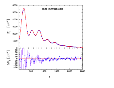
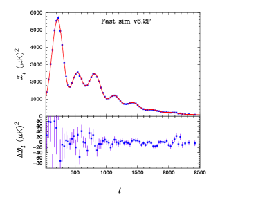
The estimates of the Planck cross-spectra are linear combinations of the pseudo- estimates, so their covariance matrices are given by e.g.,
| (46) |
Analytic expressions for these covariance matrices have been given in Efstathiou (2004, 2006); Hamimeche & Lewis (2008), and are described in Appendix A.2. The covariance matrices are computed assuming a fixed fiducial theoretical model including an unresolved foreground model for each frequency combination. Typically, the unresolved foregrounds introduce corrections to the covariance matrices of a few percent in the transition region between signal and noise domination. In addition, we compute the fiducial model by applying appropriate beam functions for each detector combination.
As discussed above, the number of coupling matrices required to compute expressions such as Eq. 46 scales as and so becomes prohibitively expensive as the number of cross-spectra becomes large. However, most of these coupling matrices are similar, differing primarily in the amplitude of the noise levels and in minor respects such as a small number of missing pixels. We can therefore adopt the same masks and weightings for groups of cross-spectra and compute coupling matrices only for distinct combinations. This dramatically reduces the computational burden. A similar approach was adopted by Lewis (2008) to analyse the WMAP 5-year temperature maps.
It is also straightforward to calculate covariance matrices for differences between different averages. If we form two spectra averaging over different detector combinations
| (47) | |||||
| (48) |
then the covariance matrix of the difference is simply
| (49) | |||||
As a pedagogical illustration of the importance of these correlations, we show in Fig. 42 two toy power spectra drawn from a Gaussian distribution with mean given by a CDM spectrum and covariance given by . That is, these spectra are not computed from a real sky map, but simply drawn directly from the error model, and therefore exclusively contain correlations modelled by the covariance matrix. The apparent “coherent oscillatory features” seen in the difference spectra (bottom panels) are therefore fully described by the CamSpec covariance matrix, accounting for correlated beam and foreground uncertainties, mask-induced coupling etc. The left panel shows a typical realisation, while the case in the right panel is selected as, visually speaking, one of the most “peculiar” within a relatively small set of simulatoins. When assessing the statistical significance of “unexpected features” in the real CMB spectrum, e.g., similar to those seen in Figs. 15 and 16, it is critical to account for these correlations.
A.5 The “fiducial Gaussian” approximation
We use a likelihood based on the so-called “fiducial Gaussian” approximation. Here we present our justification for this choice, based on an “expansion in covariance” of the exact likelihood in the exact full-sky, isotropic noise case.
Assuming the CMB, noise, and foregrounds are Gaussian, then the probability distribution for the coefficients of a collection of maps, given a model, is , where
| (50) |
up to a model-independent normalization.Here is the matrix of empirical spectra at a given multipole, and are their expectation values for the model in question.
Now, a key point to note is that theoretical power spectra typically differ from each other at each by less than they differ from the observed , because of cosmic variance and noise in the latter. So we are justified in expanding Eq. 50 about a reasonable fiducial model. Considering a single value of for simplicity, writing
| (51) |
we obtain
| (52) | |||||
to second order in . We may now complete the square in after extracting a term that is small if the fiducial model is accurate. Up to terms independent of , we have, to second order in :
| (53) | |||||
Here we have recombined the perturbation and the fiducial model back together, using Eq. 51, in the second term to obtain exactly the “fiducial Gaussian” likelihood. The first term is a correction to the fiducial Gaussian likelihood that is typically small if the fiducial model is accurate.
One can motivate neglecting this term by noticing that in its absence the approximate likelihood is unbiased (as the exact one is). One trades getting second derivatives exactly right in the vicinity of the fiducial model with getting the position, though not the depth, of the minimum right.
Vectorizing the distinct elements of (following Appendix A of Hamimeche & Lewis 2009), and recognizing the coefficients as the inverse covariance matrix elements of the spectra under the fiducial model, we obtain
| (54) |
where is the fiducial covariance matrix of the spectra, and the upper indices run on the different pairs of frequencies.
This suggests an easy generalization to the coupled cut sky pseudo-spectra, given our calculation of their covariances in Appendix A.2. We now replace the power spectra above with corresponding appropriate averages of detector cross-spectra. With bold face now denoting spectra laid out as vectors, and the grand fiducial covariance, our final action is:
| (55) |
Another advantage of the “fiducial Gaussian” approximation is that instrumental uncertainties (calibration errors, beam errors, etc.) do not appear in the inverse covariance, but only in the expression of the theoretical spectra in Eq. 55 above.
Note that if we fix the foreground model for each spectrum , together with the calibration coefficients and beam parameters, we can minimize the likelihood (Eq. 55) with respect to a ‘best-fit’ primary CMB spectrum. This ‘best-fit’ spectrum is given by the solution of
| (56) |
where the are spectrum effective calibration factors (see Appendix A.7). The covariance matrix of the estimates is given by the inverse of the Fisher matrix:
| (57) |
A.6 Uncertainties on individual detector sets beams and calibrations
Let us consider two detectors (or detector sets) and . Neglecting instrumental noise, the cross-spectrum is related to the true one, , through
| (58) |
where is the effective beam window function. Note that because of the optical beam non-circularity and the Planck scanning strategy, when , while for any and . In the range of interest, , so we denote , following the usual prescription for simple (circular) beam models. In what follows, we will drop the pair superscript except when they are required for clarity.
Our analyses use the best estimated of the sky power spectrum, where the measured is corrected by a nominal effective window :
| (59) |
The ratio , which determines the uncertainty on the angular power spectrum due to the beam, is estimated using Monte-Carlo simulations of planet transits.
We estimate and from the Monte Carlo simulations as
| (60) | ||||
| (61) |
and compute the deviations around the mean
| (62) |
Since the relative dispersion of the simulated is small (less than 1%), the deviations are well approximated by
| (63) |
The matrix then has rows and columns. Its Singular Value Decomposition (SVD) is given by
| (64) |
where is an orthogonal matrix (i.e., ), is a diagonal matrix with non-negative eigenvalues, and is a matrix with rows whose columns are orthonormal vectors (i.e., ). Here is the identity matrix.
The covariance matrix of the beam deviations is defined as
| (65) |
from which we compute the eigenmode matrix
| (66) |
using the SVD of . Most of the statistical content of or is limited to the first few modes with the largest eigenvalues. We therefore keep only the largest of the matrix. The beam uncertainty for a given spectrum is then given by
| (67) |
where is a vector of independant Gaussian variates of unit variance with elements, and is the -th row of .
This can be generalized to a set of spectra. Taking three pairs of detector sets , and , one can write
| (68) |
and the covariance matrix is given by
| (78) |
The beam errors can therefore be correlated (and in fact are strongly so, see Planck Collaboration VII 2013). In the next Appendix, this general covariance matrix is used to derive the beam error eigenmodes of combined spectra for the CamSpec likelihood.
A.7 Calibration and beam uncertainties for the CamSpec likelihood
Four effective cross-spectra are used in the CamSpec likelihood, each using an individually-prescribed -range. For each of the effective power spectra, all eligible mask- and beam-deconvolved cross-spectra are used, weighted according to
| (79) |
with labelling the effective spectrum. As describe in Appendix A.6, uncertainties in the determination of the HFI effective beams are described in terms of beam eigenmodes, , and distributions of the coresponding eigenvalues. To propagate beam errors into the likelihood, we start by using the eigenvalues, along with the weights, to construct an appropriate covariance matrix for the effects of beam errors in :
| (80) |
where is the correlation between the th eigenmode of the cross-spectrum with the -th eigenmode of the cross-spectrum. The portion of this matrix corresponding to the -range used in the likelihood is then extracted, and itself singular-value-decomposed. We keep the first (typically five) eigenmodes , , orthogonal over the -range and normalized such that the sum of their outer product directly approximates the covariance:
| (81) |
The eigenmodes are illustrated in Fig. 43.
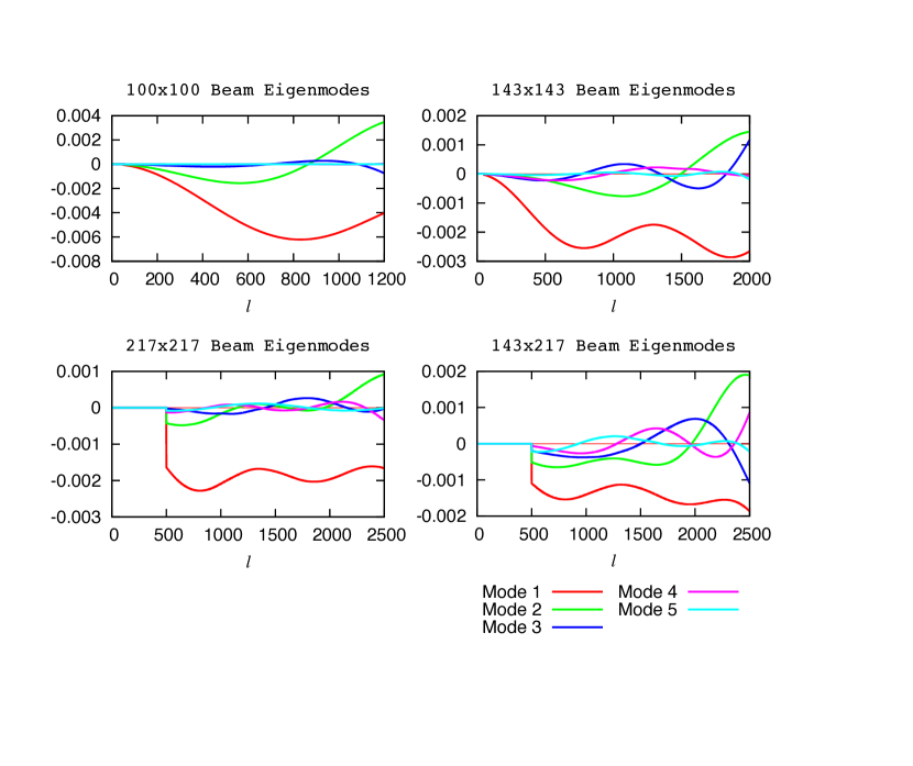
Next we calculate a suitable covariance matrix between the eigenmodes. This requires the (non-diagonal in ) inter-effective-spectrum covariance matrices , given by:
| (82) |
Given these matrices, we can “stack” the effective spectra to form a data vector and form a grand beam-covariance matrix . has length . Zero-extending each eigenmode at both ends, and arranging these into a matrix, we can form an by matrix of extended eigenmodes, , where . Now we imagine approximating as a correlated outer product of ,
| (83) |
Requiring that the covariance be chosen to minimize the summed squared-difference between elements on the two sides yields:
| (84) |
The ’s and the associated covariance are then passed to the likelihood.
A.8 Noise model of HFI detector sets
For strictly uncorrelated pixel noise , and pixel weights , the noise power spectra for the temperature maps are:
| (85) |
with contribution to the pseudo-Cℓ estimates, for uncorrelated noise, of
| (86) |
Values for are listed in Table 10. There is a significant dispersion in the noise properties of the two maps at 100 GHz. At 143 and 217 GHz, the PSB maps have significantly lower noise than the SWB maps by a factor of two, as expected.
| Map | Mask | |
|---|---|---|
| 100-ds1 | 3 | |
| 100-ds2 | 3 | |
| 143-5 | 1 | |
| 143-6 | 1 | |
| 143-7 | 1 | |
| 143-ds1 | 1 | |
| 143-ds2 | 1 | |
| 217-1 | 1 | |
| 217-2 | 1 | |
| 217-3 | 1 | |
| 217-4 | 1 | |
| 217-ds1 | 1 | |
| 217-ds2 | 1 |
The noise spectra for the Planck HFI maps are non-white. The following -parameter function
| (87) |
is a flexible parameterization that provides accurate fits for all of the HFI channels. The first term on the left models the excess ‘1/f’-like noise while the second term models the ‘bell shaped’ noise spectrum at high multipoles introduced by time constant deconvolution applied to the time-ordered data, and the low-pass filter designed to remove high-frequency noise due to demodulation. Estimates of the noise spectra can be computed from difference maps constructed from different half-ring surveys 131313As described in the HFI Data Processing paper Planck Collaboration VI (2013), these difference maps provide an estimate of the noise level in the sum maps with an accuracy of about .. Examples of fits to noise spectra for the and channels are shown in Figure 44. Note that the noise spectra are significantly non-white. At and , the deviations from white noise are smaller. Since these cross spectra contribute almost all of the weight in the likelihood at high multipoles, the modelling of non-white noise is not a critical factor in forming an accurate likelihood.
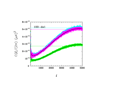
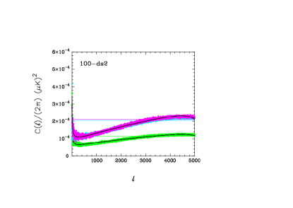
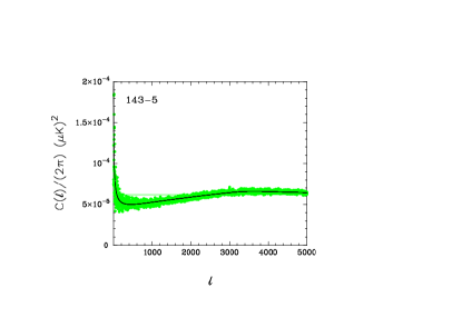
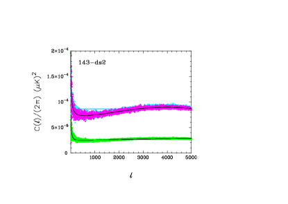
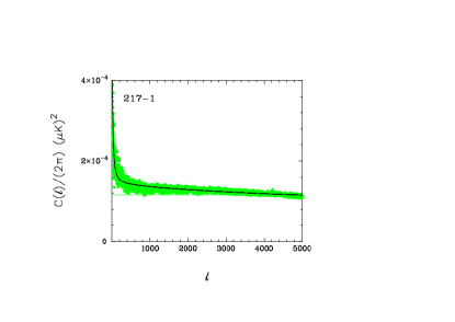
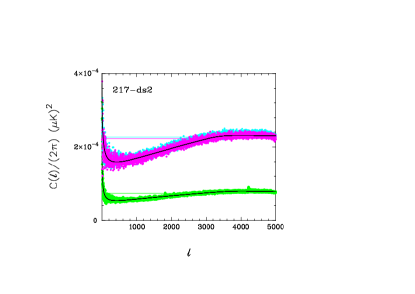
We adopt a heuristic approach to fold departures from white noise into the power spectrum covariance estimates. We define a set of noise weight functions, e.g.,
| (88) |
Wherever a term appears in a covariance matrix, we multiply the appropriate coupling matrix by a factor
| (89) |
This heuristic approach can be partially justified by noting that for isotropic Gaussian noise over the full sky, the distribution of is given by the inverse Wishart distribution:
| (90) |
where
| (91) |
e.g., Percival & Brown (2006). In this special case, our heuristic correction is exact. Further justification of the accuracy of this heuristic approach comes from direct comparisons with numerical simulations incorporating non-white noise (see Sect. 6) and from the accurate agreement of covariance matrices with the -by- scatter measured in all of the cross-spectra used to form the likelihood.
Appendix B Sky masks
We apply a threshold to the GHz temperature map to define a set of diffuse Galactic masks shown in Fig. 45. We refer to them using the percentage of the sky retained: G22, G35, G45, G56, G65. We also use a point source mask, labeled PS96, which is based on the union of the point sources detected from the channels in the range to GHz
In order to avoid power leakage, we also derive a series of apodised masks. For the Galactic masks, we proceed as follows. First, we smooth each mask with a five-degree Gaussian beam, and zero any pixels below a threshold of . We then subtract from the remaining pixels, and rescale the resulting map by . The resulting masks are shown in Fig. 46. In order to retain sufficient sky area for the most conservative sky mask, a slightly less aggressive version of mask G22 was used to seed the apodization process for that case. Each point source is apodised to 30′ FWHM, resulting in the PSA82 point source mask. A set of the resulting masks are shown in Fig. 46.
For all cosmology analyses, we use three of the apodised galactic and point sources masks: CL31, CL39, and CL49, which are shown in Fig. 2. Table 11 summarizes the various masks. For a limited set of tests in §3.2 we also used ‘mask0’ and ‘mask1’ which combine the non-apodised Galactic masks G22 and G35 with the apodised PSA82 point source mask.

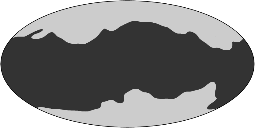

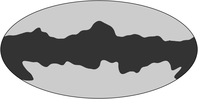
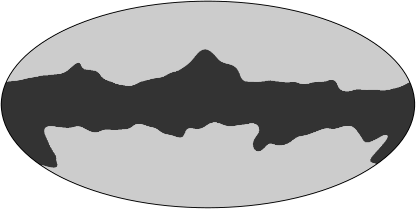
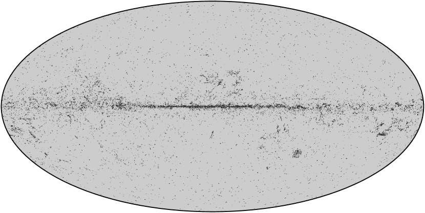
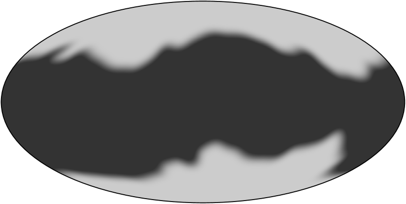


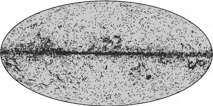
| Series Galactic Mask Apodised Galactic masks Cosmology Mask 0 G22 GA21 - 1 G35 GA34 CL31 2 G45 GA38 CL39 3 G56 GA54 CL49 4 G65 GA60 - |
Appendix C Chance correlations and inter-frequency consistency tests
Here we explicitly show that, even if the foreground contamination is much smaller than the CMB, chance cross-correlations can produce scatter in the inter-frequency power spectra that is large in the signal dominated regime. To see this, consider the case of two frequencies. Frequency 1 provides a faithful map of the CMB fluctuations. Frequency 2 contains a foreground component F. We therefore write the maps at the two frequencies as:
| (93) | |||||
| (94) |
with spherical transforms
| (2) | |||||
| (3) |
The power spectra of the two maps are therefore:
| (2) | |||||
| (3) | |||||
and the difference between the power spectra is
| (1) |
If the CMB is uncorrelated with the foreground, the first term will average to zero over a large number of CMB realizations. But we observe only one realization of the CMB, and so the cross-term will dominate the inter-frequency residuals even if the foreground contamination is much lower than the CMB (). This is the origin of the excess scatter between the and GHz power spectra at low multipoles shown in Fig. 10.
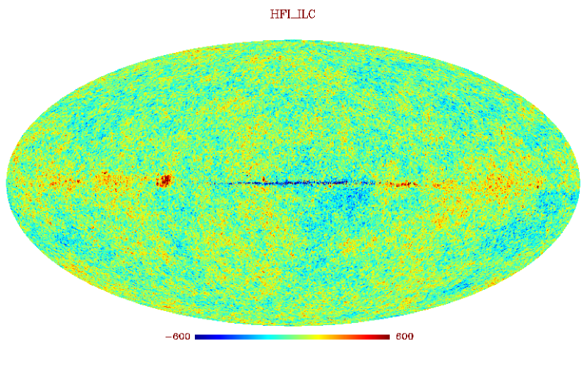
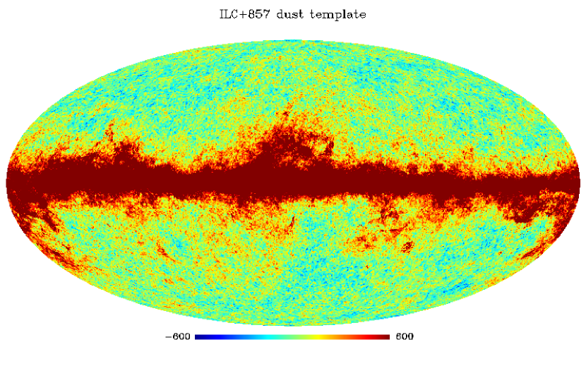
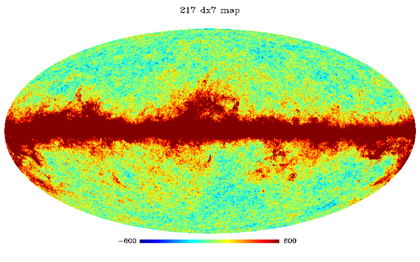
We construct a specific example of this. The upper map in Fig. 47 shows an ILC map, estimating the CMB, generated from the , , , and GHz maps. The map in the middle panel shows a ‘fake’ 217 GHz map, i.e. the sum of the ILC map and the GHz map scaled in amplitude to match dust emission at 217 GHz. The real GHz map is shown in the lower panel of Figure 47. The ‘fake’ 217 GHz map is evidently quite a good match to the real GHz. By rescaling the GHz map to estimate the dust emission at GHz, we can generate a ‘fake’ 143 GHz map in an analogous way. These ‘fake’ maps each contain two components by construction, and so the inter-frequency residuals from these maps will be dominated by the CMB-foreground cross term in Eq. 1.
The and GHz power spectrum difference from these fake maps are compared to the residuals of the real data in Fig. 48. The magenta points show the same mask1-mask0 double-difference power spectrum between and GHz as shown in Fig. 3. The only difference here is that the smoothed dust fit of Eq. 9 has been subtracted from the spectra so that the points scatter around zero. There are advantages to using the double difference because: (a) it is insensitive to calibration differences between frequencies; (b) the contrast between dust emission and other foregrounds (point sources/SZ) is stronger in the area of sky defined by mask1 - mask0 and so the double difference power spectrum should be closer to the results from the fake maps, which use only a dust template141414Actually, as demonstrated in Fig. 5, the CIB dominates over Galactic dust emission over most of the area of mask0, but this will not be a precise template for the CIB emission at cosmological channels: (a) because the spectrum of the CIB differs slightly from Galactic dust; (b) the CIB emission decorrelates from high to low frequencies because lower frequencies probe galaxies at higher redshifts. . The solid green line shows the double difference power spectrum computed from the fake maps. The amplitude of the scatter from the fake maps and the real data are very similar. In fact, there is almost point-by-point agreement between the results from the real data and the fake maps. This provides compelling evidence that the observed inter-frequency scatter at low multipoles is dominated by the CMB-foreground cross term in Eq. 1 rather than some mysterious systematic effect in the data.
The blue points in Figure 48 show the difference of the and GHz power spectra for mask1. The scatter at multipoles is almost identical to the scatter of the purple points, but increases slightly at higher multipoles. This behaviour is expected and is caused by the additional foreground components (CIB/point sources/SZ) which become comparable in amplitude to Galactic dust at multipoles greater than a few hundred.
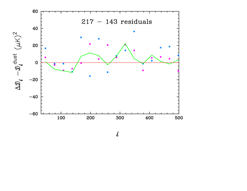
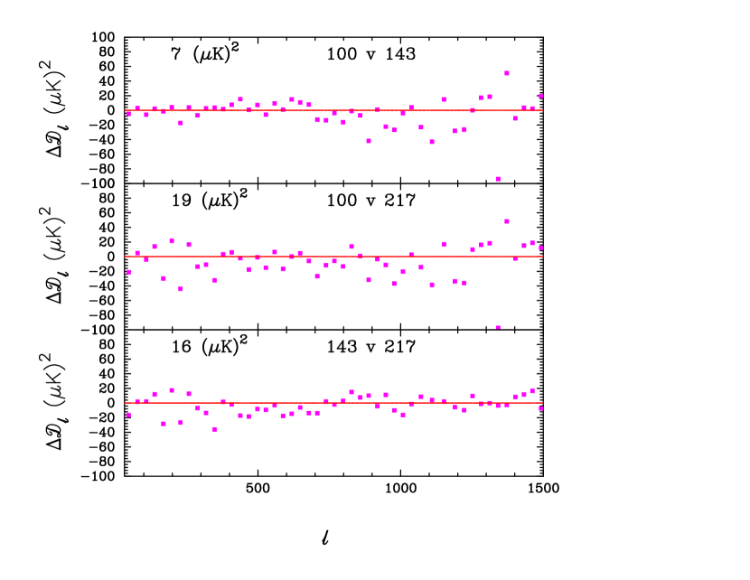
We would also expect a strong dependence of the inter-frequency residuals with frequency at low multipoles. Diffuse Galactic emission rises steadily in amplitude from GHz to GHz and hence we would expect the inter-frequency scatter to rise as we go up in frequency. This is what we see in the real data (shown in Fig. 49). Since diffuse Galactic emission is well approximated by the 857 GHz map at all frequencies, we can predict the scatter seen in this figure by scaling 857 GHz to lower frequencies. For GHz we observe a scatter of over the multipole range . So, from the GHz scalings to lower frequencies we predict the scatter given in the Table, which is in excellent agreement with the scatter seen in Figure 49.
| Predicted scatter | Observed scatter | |
|---|---|---|
| 100 - 143 | ||
| 100 - 217 | ||
Appendix D Validity tests
D.1 Detailed Validity checks
In this appendix we show the full set of figures for the distribution of the cosmological and foreround model parameters for the suite of tests described in Sect. 7. We also show the correlation matrix between these parameters and the calibration coefficents of each detector.
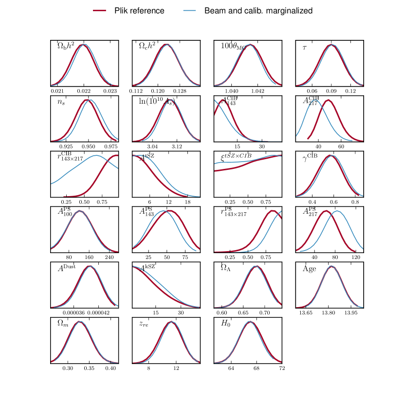
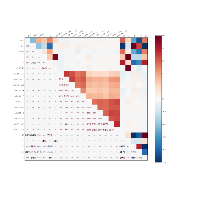
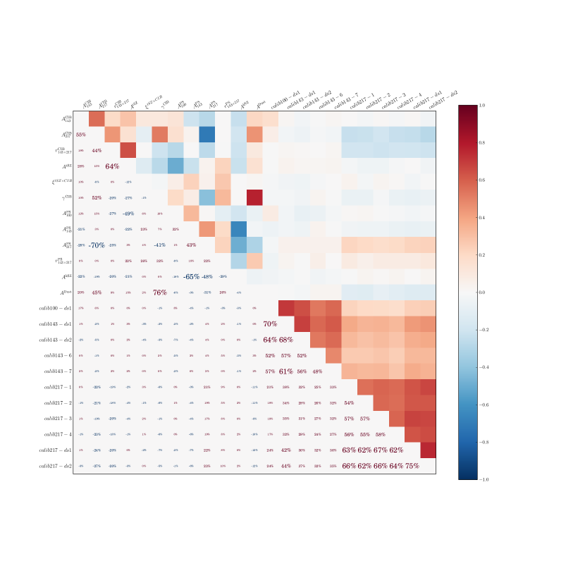
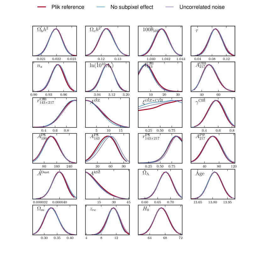
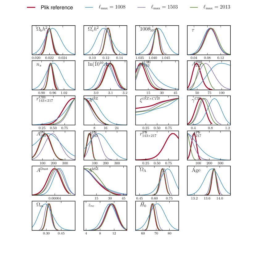
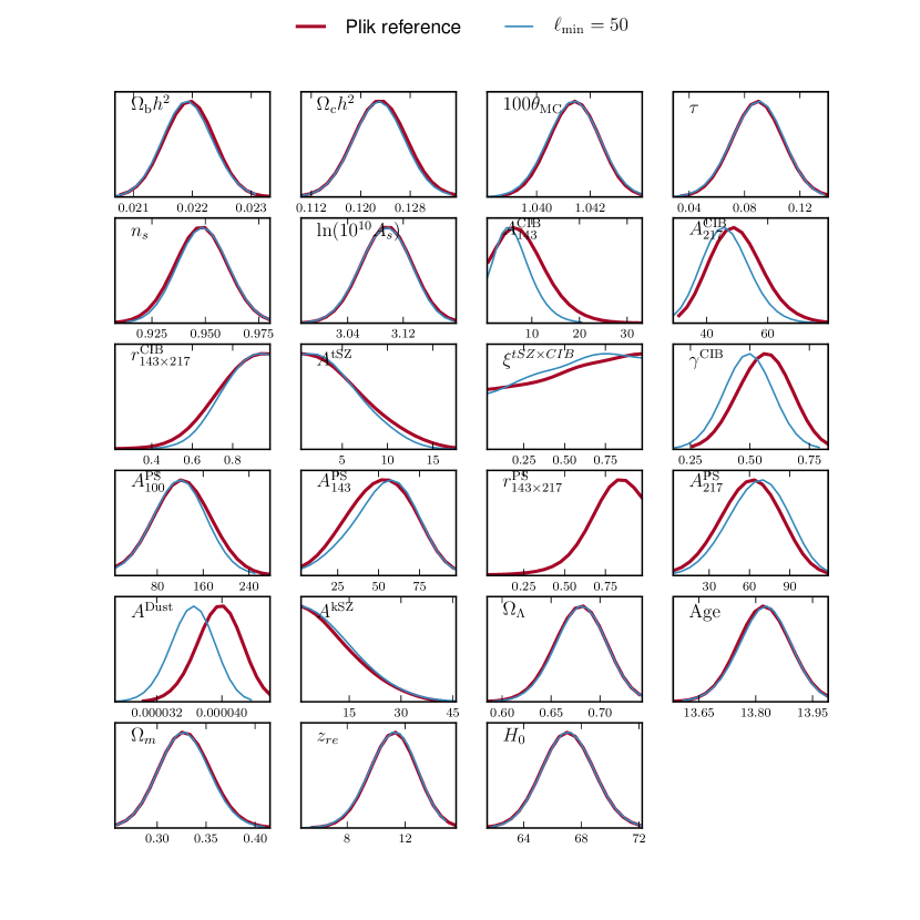
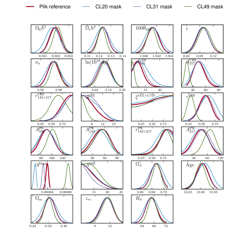
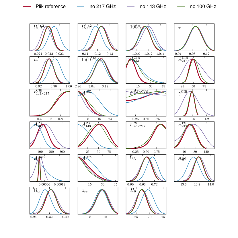
D.2 Cosmological parameters from Planck 70 GHz data
For this analysis we implement the pseudo- method described in Hivon et al. (2002) extended to derive both auto- and cross-power spectra from the 70 GHz maps (see, e.g. Polenta et al. 2005, for a comparison between the two estimators). The noise power spectrum and the covariance matrix are computed using 1000 realistic Planck simulations (FFP6, Planck Collaboration I 2013) of both signal and noise maps. The beam window functions are presented in Planck Collaboration IV (2013), and mode-coupling kernels to correct for incomplete sky coverage are computed from formulae analogous to those in Appendix. A.1.
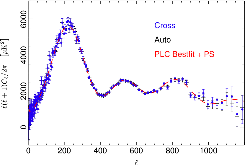
In Fig. 58 we show the auto- and cross-power spectra computed from the 70 GHz maps, where cross-spectra are obtained by cross-correlating maps from different pairs of horns (there are three such pairs in total). We use these to construct a likelihood at by assuming a Gaussian distribution for the band-powers, and include the covariance matrix estimated from simulations. To estimate cosmological parameters we use this likelihood in combination with the Planck low- likelihood. We marginalize over a single extragalactic foreground parameter, which is a Poisson term modeling unresolved residual point sources. Fig. 59 shows the resulting parameters, compared to those from CamSpec. Considering the different range contributing to the two analysis, the parameter distributions are consistent. In Fig. 60, we show 70 GHz parameters for three choices of the maximum considered: , , and . The latter two are consistent. Minor discrepancies are displayed at , which can be explained since there is, in this range, no detection of the point source component. In the same figure, we show results using the Plik likelihood for , which is consistent with Planck 70 GHz over the same range.
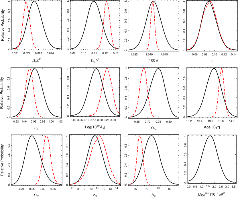
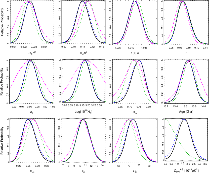
D.3 Consistency of the Planck low resolution CMB maps
Here we extend the discussion presented in Sect. 8.3. In Fig. 61 we show the power spectrum of the residual maps, relative to Commander, for NILC, SEVEM, and SMICA. The maximum discrepancy in the range (the multipole where noise begins to become non-negligible) is localized at the quadrupole and is less than , whereas for the range the differences are of order . Overall, the Planck maps are more in agreement among themselves than with WMAP, except perhaps at the quadrupole. The residual map between WMAP and Planck shows power spectrum residuals from up to to . These figures should be compared to the residual estimated from simulated foreground maps, shown to be at in Planck Collaboration XII (2013).
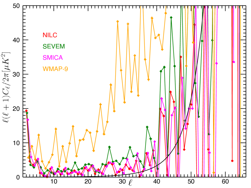
We complement our results with those obtained from the ‘FFP6’ simulations described in Planck Collaboration XII (2013). They consist of signal plus noise maps processed through each of the four component separation pipelines.
For each Monte Carlo realization, we follow the same procedure as in the previous section, i.e. smoothing () and binning the maps to . We apply this procedure to both the CMB input maps and the output maps derived by the four component separation algorithms. Again, a Gaussian white noise with a variance of is added, and the noise covariance matrix is corrected accordingly. Note that the additional white noise is taken into account not only for numerical regularization (to this extent its amplitude may well be lower), but principally because the output instrumental noise processed through component separation and downgraded to low resolution is far from being white. The additional white noise makes the detailed knowledge of the full noise covariance matrix unimportant.
For each realization and for each component separation code, we compute the power spectrum of the processed map and of the input signal map, using a common mask. When estimating the power spectrum, the input CMB maps are regularized by adding a negligible Gaussian white noise with variance. We have checked explicitly that when the white noise is added to the component separated maps, we are able to recover the input power spectrum without bias up to for all the four component separation methods.
Moreover, we compute the power spectrum of the difference maps (output processed map minus input CMB) for each realization, in order to evaluate the total amount of residual noise. Note that this is not only given by the added regularization noise, but also from the intrinsic noise, albeit small, that is present in the maps.
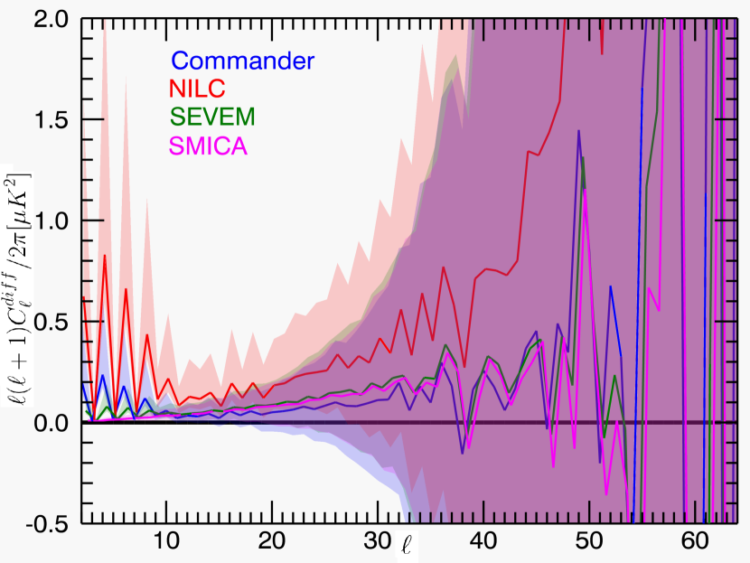
Fig. 62 shows the average and the levels of such noise residuals for each of the component separation solutions. We thus see, that the level of such total noise residuals is well below the difference plotted in Fig. 61. Therefore, we argue that the existing differences between the codes are due to genuine foreground separation residuals.
Appendix E Dust cleaning using Planck 353 GHz
The WMAP polarization products are weighted combinations of Ka, Q, and V band 9 year maps. The WMAP analysis mitigates polarized foreground emission using template fitting, with synchrotron and dust foregrounds. As a template for synchrotron emission, the WMAP K band channel is used, and for dust a polarization model is used to create a template map (Page et al. 2007). Here we assess the impact on the WMAP polarization signal when this dust template is replaced by the Planck 353 GHz map, which can be assumed to trace the dust better. This is only for comparison; we continue to use the WMAP polarization products as released by the WMAP team (except using the Planck map as discussed in Sect. 8).
Foreground cleaned maps can be written as
where are linear polarization Stokes parameter maps, and the index is for Ka, Q, and V bands. Here is the WMAP 9-year K band map and for we use either the WMAP dust template or the Planck 353 GHz maps. For each frequency band, the scaling coefficients and are estimated by minimizing the :
| (2) |
where is the covariance matrix. Following the WMAP analysis, we do not include the signal contribution in and we only use the diagonal elements of the noise covariance matrix to estimate . Scaling coefficients are computed using two different WMAP masks: the ‘processing mask’ that masks a narrow region in the plane of the Galaxy, and the more conservative ‘P06’ mask used for power spectrum estimation and cosmological analysis.
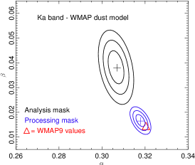
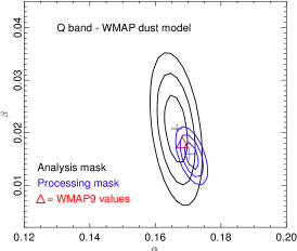
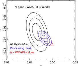
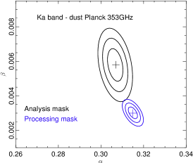
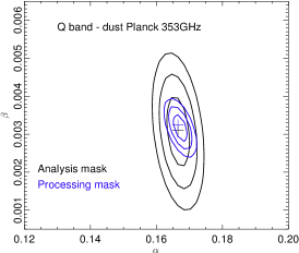
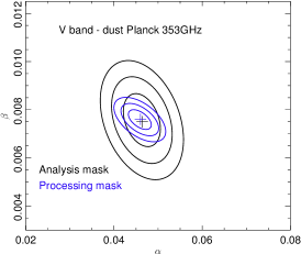
The template coefficients at each channel are shown in Fig. 63, estimated using the two different Galactic masks. At Q and V band the estimated coefficients are consistent for the two masks; at Ka band the 353 GHz map gives more consistent results than the WMAP dust template. The coefficients using the P06 mask are more uncertain however, as the residual dust signal outside the mask is low, especially for Ka band. We find that the preferred synchrotron coefficient, , is slightly lower using the 353 GHz map, and the overall , shown in Table 12, is slightly improved using the Planck dust map.
| Ka | Q | V | |
|---|---|---|---|
| Planck 353 GHz | 1.127 | 1.132 | 0.991 |
| WMAP dust model | 1.135 | 1.149 | 1.030 |
We test the effect on cosmological parameters, in particular the optical depth to reionization, using the two different templates. Using the Planck 353 GHz channel as the dust template, with coefficients estimated using the processing mask, lowers the best fit value of by about 1 (see Fig. 64). we find , compared with using the WMAP dust model. This also has the effect of lowering , from to , but other CDM parameters are not affected. We note though that using template coefficients estimated outside the P06 Galactic mask, the optical depth using the Planck template is lowered by only compared to the WMAP template, indicating some spatial dependence. We conclude that the impact on cosmological parameters from the choice of dust template is not significant, but anticipate more extensive analysis with the full Planck polarization data set.
