Dark torsion as the cosmic speed-up
Abstract
It is shown that the recently detected acceleration of the universe can be understood by considering a modification of the teleparallel equivalent of General Relativity (TEGR), with no need of dark energy. The solution also exhibits phases dominated by matter and radiation as expected in the standard cosmological evolution. We perform a joint analysis with measurements of the most recent type Ia supernovae (SNe Ia), Baryon Acoustic Oscillation (BAO) peak and estimates of the CMB shift parameter data to constraint the only new parameter this theory has.
pacs:
Valid PACS appear hereI Introduction
The discovery of an unexpected diminution in the observed energy fluxes coming from type Ia supernovae perlmutter-otros ; kowalski has opened one of the most puzzling and deepest problems in cosmology today. These observations have been interpreted as solid evidence for an accelerating universe dominated by something called dark energy. Although the cosmological constant seems to be the simplest explanation for the phenomenon, several dynamical scenarios have been tried out since 1998 (see e.g., sahni ; padma ; frieman ). While some authors sustain the idea of the existence of a dark energy, others propose modifications of the Einstein-Hilbert Lagrangian known as (buch ; staro ; ker ; barrow1 ; barrow2 ; carroll ; starobinsky ; hu ; odintsov1 or odintsov2 ; capo ; sotiriou for recent reviews) as a way to obtain a late accelerating expansion. A great difficulty these theories have, from the point of view of the metric formalism, is that the resulting field equations are 4th order equations, which in many cases makes these hard to analyze. Besides, the simplest cases of the kind have shown difficulties with, weak field tests chiba ; olmo , gravitational instabilities dolgov and do not present a matter dominated era previous to the acceleration era amendola1 ; amendola2 . Alternatively, the Palatini variational approach for such theories leads to 2nd order field equations, and some authors have achieved to put observational constraints to these theories amar ; fay ; santos . However in many cases the equations are still hard to work with, as evidenced by the functional form of the modified Friedmann equation for a generic . Recently, models based on modified teleparallel gravity were presented as an alternative to inflationary models franco ; franco2 . In this paper we show a cosmological solution for the acceleration of the universe by means of a sort of theories of modified gravity, namely , based on a modification of the teleparallel equivalent of General Relativity (TEGR) Lagrangian einstein ; hayashi where the torsion will be the responsible of the observed acceleration of the universe, and the field equations will always be 2nd order equations.
II General considerations. Field equations
Teleparallelism einstein ; hayashi uses as dynamical object a vierbein field , , which is an orthonormal basis for the tangent space at each point of the manifold: , where . Each vector can be described by its components , in a coordinate basis; i.e. . Notice that latin indexes refer to the tangent space, while greek indexes label coordinates on the manifold. The metric tensor is obtained from the dual vierbein as . Differing from General Relativity, which uses the torsionless Levi-Civita connection, Teleparallelism uses the curvatureless Weitzenböck connection weit , whose non-null torsion is
| (1) |
This tensor encompasses all the information about the gravitational field. The TEGR Lagrangian is built with the torsion (1), and its dynamical equations for the vierbein imply the Einstein equations for the metric. The teleparallel Lagrangian is hayashi ; maluf ; arcos ,
| (2) |
where:
| (3) |
and is the contorsion tensor:
| (4) |
which equals the difference between Weitzenböck and Levi-Civita connections.
In this work the gravitational field will be driven by a Lagrangian density that is a function of . Thus the action reads
| (5) |
where . The case corresponds to TEGR. If matter couples to the metric in the standard form then the variation of the action with respect to the vierbein leads to the equations
| (6) |
where a prime denotes differentiation with respect to , and is the matter energy-momentum tensor. The fact that equations (6) are 2nd order makes them simpler than the dynamical equations resulting in theories.
III Cosmological solution and observational constraints
We will assume a flat homogeneous and isotropic FRW universe, so
| (7) |
where is the cosmological scale factor. By replacing in (1), (3) and (4) one obtains
| (8) |
being the Hubble parameter . As a remarkable feature, the scale factor enters the invariant just through the Hubble parameter. The substitution of the vierbein (7) in (6) for yields
| (9) |
Besides, the equation is
| (10) |
In Eqs. (9-10), and are the total density and pressure respectively. It can be easily derived that they accomplish the conservation equation
| (11) |
whatever is. Thus, if the state equation is then evolves as ( is the cosmological redshift).
We are interested in obtaining an accelerated expansion without dark energy but driven by torsion. For this we will try with a kind of theories:
| (12) |
being and real constants to be determined by observational constraints. Although the functional form of (12) is similar to those considered in literature, now the guideline towards modified gravity is instead of . This fact gives to these theories another interesting feature because is the most important cosmological variable. For later times the term is dominant, while in early times, when , General Relativity is recovered. From (9) along with (12), the modified Friedmann equation results to be
| (13) |
(a functional dependence similar to the results other authors arrived, through different theoretical motivations such as dvali ; goobar ).
Now, replacing , and calling the contributions of matter and radiation to the total energy density today, Eq. (13) becomes
| (14) |
where , and . The evaluation of this equation for allows to rephrase the constant as a function of and : . For (then ) the GR spatially flat Friedmann equation is retrieved. The case recovers the GR dynamics with cosmological constant . Notice the functional simplicity of (13) compared with its analogue in theories. Compared with GR, is the sole new free parameter in (14), since specifying the value of and () the value of (in units of ) is automatically fixed through the relation (13). In order to obtain we solve numerically the equation (14).
Since the most solid evidence for the acceleration of the universe comes from measurements of luminosity distances for type Ia supernovae, we will use the most recent compilation of 307 SNe Ia events (the Union sample) kowalski , to put constraints in the plane. The predicted distance modulus for a supernova at redshift , for a given set of parameters P=(, ), is
| (15) |
where and are the apparent and absolute magnitudes respectively, and stands for the luminosity distance (in units of megaparsecs),
| (16) |
where is given by the numerical solution of (14). We use a statistic to find the best-fit for a set of parameters P (marginalizing over ),
| (17) |
where is defined by (15), and are the distance modulus and its uncertainty for each observed value kowalski . As it is known, the measurements of SNe Ia are not enough to constraint thoroughly. To perform the statistic we also consider, on one hand, the information coming from the BAO (Baryon Acoustic Oscillation) peak detected in the correlation function of luminous red galaxies (LRG) in the Sloan Digital Sky Survey eisen . The observed scale of the peak effectively constraints the quantity (assumed a model),
| (18) |
where is the typical redshift of the LRG and is defined as
| (19) |
On the other hand, we have also included in the statistic the CMB shift parameter, which relates the angular diameter distance to the last scattering surface with the angular scale of the first acoustic peak in the CMB power spectrum. In order to do this, we have considered a radiation component =5 x . The CMB shift parameter is given by komatsu ,
| (20) |
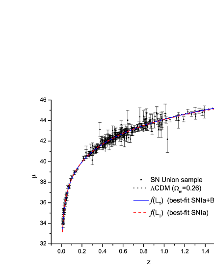
We can use both parameters since our model presents matter domination at the decoupling time. Figure 1 shows the Hubble diagram for the 307 SNe Ia belonging to the Union sample. The curves represent models with values of and obtained from minimizing using only SNIa and SNIa+BAO+CMB as well. It is also shown as a reference the model with . The obtained values for the best-fit to the SNe Ia data only are and with the reduced (or equivalently, ) where is the number of degrees of freedom.
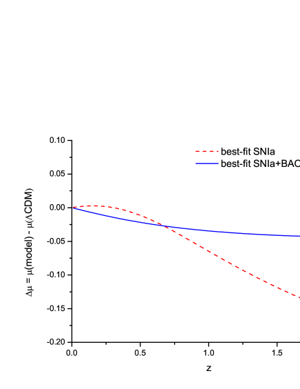
In Figure 2 we plot the distance modulus residual () from the model to better appreciate the discrepancies between our model and .
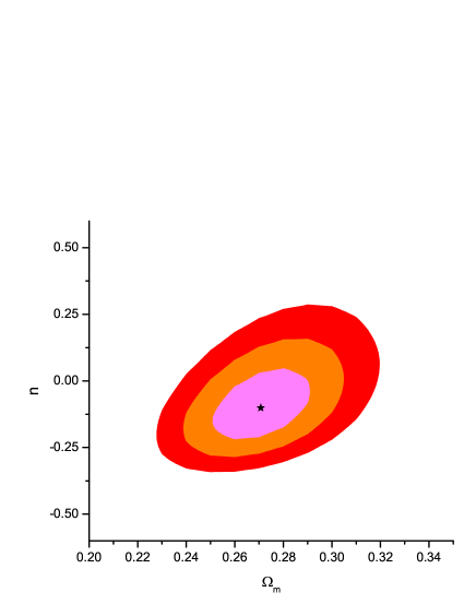
Figure 3 shows the confidence intervals at 68.3%, 95.4% and 99.7% for the joint probability of the parameters and , having combined the SNe Ia data with BAO and CMB parameters. This analysis yields that the best-fit to all data is achieved with and (with a ) and also the values of the parameters lie in the ranges (at 68.4% c.l.): [0.25, 0.29].
For our model we have analyzed as well the total and effective equations of state as a function of . From (13) and (10) along with (12), one can define a torsion contribution to the density and pressure as
| (21) | |||||
to rewrite the dynamical equations as
| (22) | |||||
| (23) |
Then, by using (22) and (23) the total and effective equations of state are written as,
| (24) |
| (25) |
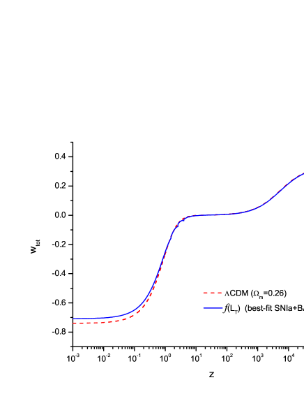
Figure 4 shows the evolution of the total equation of state as a function of for our model with the values of the best-fit. There can be observed the last three phases of the evolution of the universe: radiation dominated (), matter dominated () and late acceleration (). Figure 5 shows the effective equation of state coming from the dark torsion contribution. Finally, analyzing (23) we find that our model with predicts that the transition from deceleration to acceleration occurs at in good agreement with recent works melch07 .
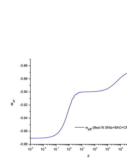
An interesting point to be highlighted is that equation (13) reveals that a value of , as the one obtained by considering only SNIa data, implies that the effective dark torsion is of the phantom type cal02 . That is, since decreases toward the present time, the dark torsion density increases instead of diluting with expansion (). However, when combining the complete data with SNIa+BAO+CMB we can see from Fig. 3 that it is slightly favored ( c.l.) a model with .
IV Conclusions
A theory based on a modification of the teleparallel equivalent of General Relativity (TEGR) -where torsion is the geometric object describing gravity instead of curvature and its equations are always of 2nd order- is remarkably simpler than theories. We have tested the theory with the aim of reproducing the recently detected acceleration of the universe without resorting to dark energy. We have here performed observational viability tests for this theory by using the most recent SN Ia data, and combined them with the information coming from BAO peak and CMB shift parameter in order to find constraints in the plane. At 68.3% c.l. we found that the values lie in the ranges and . The values for are consistent with recent estimations obtained by other authors (see, e.g., spergel ). The model with the best-fit values minimizing the that combines SNIa+BAO+CMB data ( and ) exhibits the last three phases of cosmological evolution: radiation era, matter era and late acceleration; this last stage having started at .
Acknowledgements.
G.R.B. is supported by a CONICET graduate scholarship. G.R.B thanks Franco Fiorini for his encouraging at the early stages of the work. Both authors are grateful to Diego Travieso, Gastón Giribet and Susana Landau for helpful discussions. This work was partially supported by CONICET.References
- (1) Perlmutter S. et al., Bull. Am. Astron. Soc. 29, (1997) 1351; Astrophys. J. 517, (1999) 565; Riess A. G. et al., Astrophys. J. 116, (1998) 1009; Astrophys. J. 607 (2004) 665.
- (2) Kowalski M. et al., Astrophys. J. 686, (2008) 749.
- (3) Sahni V. and Starobinsky A. A., Int. J. Mod. Phys. D9, (2000) 373.
- (4) Padmanabhan T., Phys. Rep. 380, (2003) 235.
- (5) Frieman J., Turner M. S. and Huterer D., Dark Energy and the Accelerating Universe, arXiv:0803.0982.
- (6) Buchdahl H. A., Mon. Not. R. Astron. Soc. 150, (1970) 1.
- (7) Starobinsky A. A., Phys. Lett. B91, (1980) 99.
- (8) Kerner R., Gen. Relat. Gravit. 14, (1982) 453.
- (9) Barrow J. D. and Ottewill A. C., J. Phys. A: Math. Gen. 16, (1983) 2757.
- (10) Barrow J. D. and Cotsakis S., Phys. Lett. B214, (1988) 515.
- (11) Carroll S. M. et al., Phys. Rev. D70, (2004) 043528.
- (12) Starobinsky A. A., JETP Lett. 86, (2007) 157.
- (13) Hu W. and Sawicki I., Phys. Rev. D76, (2007) 064004.
- (14) Nojiri S. and Odintsov S. D., Dark energy, inflation and dark matter from modify f(R) gravity, ArXiv:0807.0685.
- (15) Nojiri S and Odintsov S. D., Int. J. Geom. Meth. Mod. Phys. 4, (2007) 115.
- (16) Capozziello S. and Francaviglia M., Gen. Relat. Gravit. 40, (2008) 357.
- (17) Sotiriou T. and Faraoni V., f(R) theories of gravity, arXiv:0805.1726.
- (18) Chiba T., Phys. Lett. B575, (2003) 1.
- (19) Olmo G., Phys. Rev. Lett. 95,(2005) 261102.
- (20) Dolgov A. and Kawasaki M., Phys. Lett. B573, (2003) 1.
- (21) Amendola L. et al., Phys. Rev. Lett. 98, (2007) 131302.
- (22) Amendola L. et al., Phys. Rev. D75, (2007) 083504.
- (23) Amarzguioui M. et al., Astron. and Astrophys. 454, (2006) 707.
- (24) Fay S., Tavakol R. and Tsujikawa S., Phys. Rev. D75, (2007) 063509.
- (25) Santos J. et al., Phys. Lett. B669, (2008) 14.
- (26) Ferraro R. and Fiorini F., Phys. Rev. D75, (2007) 084031.
- (27) Ferraro R. and Fiorini F., Phys.Rev. D78, (2008) 124019.
- (28) Einstein A., Sitzungsber. Preuss. Akad. Wiss. (1928) 217; ibid., (1930) 401; Einstein A., Math. Annal. 102, (1930) 685.
- (29) Hayashi K. and Shirafuji T., Phys. Rev. D19, (1979) 3524, Addendum-ibid. D24, (1982) 3312.
- (30) Weitzenböck R., Invarianten Theorie, (Nordhoff, Groningen, 1923).
- (31) Maluf J. W., J. Math. Phys. 35, (1994) 335.
- (32) Arcos H. and Pereira J., Int. J. Mod. Phys. D13, (2004) 2193.
- (33) Dvali G. and Turner M. S., Dark Energy as a Modification of the Friedmann Equation, ArXiv:astro-ph/0301510.
- (34) Fairbairn M. and Goobar A., Phys. Lett. B642, (2006) 432.
- (35) Eisenstein D. et al., Astrophys. J. 633, (2005) 560.
- (36) Komatsu E. et al., Astrophys. J. Suppl. 180, (2009) 330.
- (37) Melchiorri A. et al., Phys. Rev. D76, (2007) 041301(R).
- (38) Caldwell R. R., Phys. Lett. B545, (2002) 23.
- (39) Spergel D. N. et al., Astrophys. J. Suppl., 148, (2003) 175; Astrophys. J. Suppl., 170, (2007) 377.