Frequency domain reduced order models for gravitational waves from aligned-spin compact binaries
Abstract
Black-hole binary coalescences are one of the most promising sources for the first detection of gravitational waves. Fast and accurate theoretical models of the gravitational radiation emitted from these coalescences are highly important for the detection and extraction of physical parameters. Spinning effective-one-body (EOB) models for binaries with aligned spins have been shown to be highly faithful, but are slow to generate and thus have not yet been used for parameter estimation studies. I provide a frequency-domain singular value decomposition (SVD)-based surrogate reduced order model that is thousands of times faster for typical system masses and has a faithfulness mismatch of better than with the original SEOBNRv1 model for advanced LIGO detectors. This model enables parameter estimation studies up to signal-to-noise ratios (SNRs) of 20 and even up to SNR 50 for total masses below . This article discusses various choices for approximations and interpolation over the parameter space that can be made for reduced order models of spinning compact binaries, provides a detailed discussion of errors arising in the construction and assesses the fidelity of such models.
pacs:
04.25.Dg, 04.25.Nx, 04.30.Db, 04.30.Tv1 Introduction
The LIGO [1] and VIRGO [2] detectors along with GEO600 [3] span a world-wide network of ground based gravitational wave detectors using laser interferometry. Currently LIGO and VIRGO are being upgraded into advanced detectors which will increase the detector sensitivities by a factor of 10 and event rates by a factor of 1000. The advanced LIGO (aLIGO) and Virgo (AdV) detectors [4, 5, 6] are due to come online in 2015-16 and expected to reach their design sensitivity around 2018 [7] when they will very likely make routine detections. The advanced detectors are expected to provide a wealth of astrophysical information (see, e.g., [8]) and help establish the field of gravitational-wave astronomy. Furthermore, an underground cryogenic detector in Japan, KAGRA [9], is under construction.
The coalescence of compact binary systems is one of the most promising sources of gravitational waves (GWs) for these detectors. The theoretical knowledge of the gravitational waveforms emitted by these sources is essential for signal detection and the determination of astrophysical parameters. The standard technique for observing compact binary coalescences involves matched filtering detector data against a set of “template” waveforms which approximate potential astrophysical signals [10]. Furthermore, parameter estimation (PE) algorithms can provide estimates of the parameters of compact binary systems observed with the detection algorithms. The goal of Bayesian PE methods is to estimate the posterior probability density function of the parameters that describe the signal and to evaluate the evidence of different waveform models.
To this end the post-Newtonian (PN) expansion [11] in of Einstein’s equations provides a powerful formalism to describe these waveforms during the inspiral, when the orbital speed is much smaller than the speed of light. Binary neutron stars (BNS) are expected to accumulate the majority of the signal-to-noise ratio (SNR) in the inspiral regime and are therefore well described by high-order PN waveforms. 3.5PN order templates have been shown [12, 13] to be sufficient for searches of non-spinning compact binaries of total mass up to . For parameter estimation higher accuracy is required.
The PN expansion breaks down in the plunge, merger and ringdown phases of compact binary coalescence. As the total mass of the binary increases the detectors become more sensitive to these strong field effects that manifest themselves at higher frequency. To describe the waveforms radiated from BH binaries in these late stages of evolution numerical solutions of the full nonlinear Einstein equations are required [14]. Complete inspiral-merger-ringdown (IMR) models are created from an amalgam of PN and numerical relativity (NR) waveforms. In practice, both approaches are necessary since generating NR waveforms of more than several tens of orbits is too computationally expensive.
Two broad classes of IMR models have been proposed for BH binaries with spins aligned with the orbital angular momentum. Phenomenological models [15, 16] are constructed in the frequency domain using fits to PN-NR hybrid waveforms. This technique was used to provide models that can be evaluated very fast and are therefore suitable also for the demanding methods required for parameter estimation. In contrast, effective-one-body (EOB) models [17, 18, 19, 20, 21] use an analytical approach that combines PN expansion, re-summation techniques and perturbation theory with additional calibration of certain model parameters against NR waveforms. EOB waveforms have been shown to be very accurate (e.g. for the non-spinning EOBNRv2 model [22] uncertainties in PE are dominated by statistical rather than systematic error [23]), but are much slower to generate than the aforementioned phenomenological models since a complicated system of ordinary differential equations has to be solved over a long time interval with small time steps.
The Bayesian methods employed in PE studies require the generation of model waveforms to probe the 11 (for aligned spin binaries) dimensional parameter space [24]. The more complex EOB models, such as the spinning EOB model SEOBNRv1 [25] on which we focus in this paper, are therefore too expensive for direct use in PE calculations [24]. For example, to generate an equal-mass SEOBNRv1 waveform for a binary that fills the aLIGO band down to Hz takes about 40 seconds on a current workstation and thus a PE study assuming no parallelism may take about ten years. In this paper we present a surrogate model of SEOBNRv1 that reduces the computational cost for this example by a factor of about three thousand, making it possible to generate the waveforms for such a study on the order of a day.
Even the generation of template banks for detecting GW signals from compact binaries becomes very expensive for aligned-spin systems. Stochastic template bank placement techniques [26, 27] produce banks with a size on the order of templates [28, 29] but require the generation of further waveforms during its construction as the bank becomes denser. In contrast to PE a template bank needs to be built only once, but the cost at low total masses may again be prohibitive for complex models such as SEOBNRv1. Let us note, though, that the nonspinning EOBNR model [22] has been used in PE studies and template bank creation.
Reduced order modeling (ROM) techniques can be used to build surrogate models that provide fast and accurate compressed approximations of a selected source waveform model. Several such methods have been proposed in the literature. Singular value decomposition (SVD)-based methods have been used [30, 31, 32, 33] to interpolate time-domain inspiral waveforms. Cannon et al [34] calibrate a reduced basis of non-spinning PhenomB waveforms against a set of NR waveforms to obtain a model with improved accuracy. SVD-based methods have also been used to provide efficient representations of template banks [35, 36]. Another class of methods are greedy reduced basis (RB) methods which are usually combined with the empirical interpolation method [37]. These techniques have also been applied to GW waveforms [38, 39, 40, 41] and BH ringdown [42]. Herrmann et al [39] find that the number of RB elements needed to represent aligned-spin TaylorF2 [43, 44, 45, 12, 46]111TaylorF2 is a closed-form frequency domain PN approximant obtained via the stationary phase approximation. inspiral waveforms is not much larger than for the non-spinning case. Blackman et al [41] show that precessing PN waveforms can be represented to high accuracy in a surprisingly compact basis. Neither [39] nor [41] build an actual model. Field et al [38] build test models of the non-spinning EOBNR [22] waveform family over small mass-ratio intervals, from 1 to 2 and 9 to 10.
Further techniques have recently been proposed to help speed up parameter estimation calculations. One approach is to directly interpolate the likelihood function [47] with the help of the SVD; a different method speeds up likelihood evaluations by defining special reduced order quadrature rules [48, 49, 50]. SVD-interpolated waveforms have been shown to satisfy the stringent waveform-model accuracy criteria imposed by parameter-estimation requirements [30]. So far, reduced order models with application for searches and PE have been restricted to non-spinning waveforms and to small subregions of the mass space.
In this study I propose a method for building reduced order models covering a multi-dimensional intrinsic parameter space (mass-ratio and spins) for the first time. The emphasis is on a practical approach with a view towards data analysis requirements for the advanced detector era. To achieve this I make the following choices. The model approximates SEOBNRv1 waveforms in the frequency domain. This allows for the fast computation of waveforms and their match, which is defined as a frequency domain inner product weighted by the detector noise. A sparse set of frequency points is introduced that yields a highly accurate representation of waveforms from the BNS regime up to hundreds of solar masses. I compute reduced bases with the SVD separately for the amplitude and phase of the frequency domain waveform starting from a set of input waveforms on a regular parameter space grid. This separate treatment of amplitude and phase allows for higher compression in the model.
I first build a single-spin model over a very wide range of the parameter space, up to mass-ratio , which is way beyond the calibration range of the source model, and later a double-spin model up to . Single-spin models add one additional parameter compared to non-spinning models and are thus the simplest models describing spinning binaries and provide an ideal testbed for reduced order modeling techniques. The single-spin model only uses equal-spin waveforms and can be used as an effective single-spin model [51] similar to the approach used in phenomenological models for aligned-spin binaries [15, 16, 52]. The dimensionless spin parameters are defined as , where and are the spin and mass of companion (black hole or neutron star) .
For the sake of simplicity, all of the modeling techniques used will be discussed for the single-spin model, but can be extended to the double-spin model in a straightforward manner. I will show that the single-spin model can help identify problems in the source model beyond its calibration range. Thus, reduced order models can be used as a tool that can also be applied to assess waveforms and identify regions in the parameter space where the model should be improved. The fidelity of the reduced order models is analyzed in terms of the faithfulness mismatch against the original SEOBNRv1 model, i.e. I only optimize over time and phase shifts, but not over model parameters. When speedup and mismatch studies are carried out, the reduced order models are compared against FFTs of SEOBNRv1 waveforms without hybridization.
The outline of this paper is as follows. I will summarize the SEOBNRv1 waveform model in Section 3 and give details on how the frequency domain input waveforms are generated in Section 4. I will describe how the SVD can be used to build a reduced basis, compute projection coefficients against a set of input waveforms and give a formal description on how to assemble the surrogate waveform model in Section 6. I will then discuss different choices for interpolating the projection coefficients over the (intrinsic) parameter space in Section 8 and techniques for generating a suitable set of sparse frequency grid points in Section 5. In Section 9 I will compare errors arising from approximations introduced in building the model. Model accuracy will be studied for a single-spin model in Section 10 and double-spin model in Section 11. At the end I will compare SVD and greedy basis methods, summarize the performance and storage requirements and address future extensions of the technique in Section 12.
2 Aligned-spin SVD-based reduced order models in a nutshell
This section provides an executive summary of the speedup provided by the reduced order models discussed in this paper. It gives an overview of how the models are constructed pointing the reader to section where the various ingredients are discussed in details. At this point the reader is not expected to understand the details of each step. Finally I summarize the fidelity of the single- and double-spin models.
2.1 The need for fast surrogate models
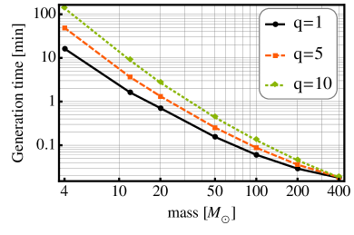
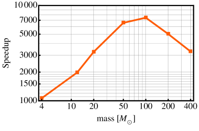
I have already pointed out in Section 1 that a fast surrogate model of SEOBNRv1 would be extremely useful for PE studies and for the construction of template banks. Let us take a closer look at the time needed for generating SEOBNRv1 waveforms at various total masses and contrast this with the increase in speed obtained from the reduced order models presented in this work. As the left panel of Figure 1 shows the generation time for SEOBNRv1 waveforms as implemented in the LSC Algorithms Library [53] (LAL) becomes very high for low total mass, from tens to hundreds of minutes if the full IMR waveform is needed. The cost also rises with mass-ratio and with sampling frequency. The evaluation speed for the surrogate models presented in this paper per frequency point is independent of the system mass, but depends on the dimensionality of the parameter space, the number of sparse frequency gridpoints used in the construction of the model (as defined in Section 5) and the dimension of the basis matrices. The speedup of the ROM vs SEOBNRv1 is summarized in the right panel of Figure 1 for equal-mass waveforms. The plot shows timings for a C implementation of the ROM; the Mathematica code is about a factor of slower.
To fully represent the FFT of a time-domain waveform of length (with power only in the positive frequencies), frequency points are required and is inversely proportional to the sampling frequency. This number of points rises to the order of millions at low total masses and the dominating cost for such large numbers of model evaluations is spline interpolation in frequency for the models discussed in this paper. For this use case a speedup of a factor of 1000 or more can be obtained in the ROM compared to SEOBNRv1. For applications in searches and parameter estimation involving detector data the full number of frequency points according to the used sample rate is needed. However, when comparing reduced order models against SEOBNRv1 in this paper it turns out that a frequency spacing of for the aLIGO frequency band (corresponding to about 10000 frequency evaluations) already yields sufficiently accurate matches222In the computation of the match (see Equation (5.2)) one maximizes over time-shifts between two waveforms to minimize the dephasing. If the peak of the correlation function is well enough resolved the match will be accurate. Zero-padding the match integrand is also very beneficial..
This massive reduction in the computational cost makes possible detailed parameter estimation studies with spinning EOB models and will be a very valuable tool in the advent of the advanced detector era. Assuming a cost of about minutes per SEOBNRv1 waveform in the BNS region and a PE study requiring (serial) waveform evaluations, the total time of the analysis would be around 280 years. Using a C implementation of the reduced order model such a study could be completed in several months using the full set of frequency points. Further speedup is possible through the use of reduced order quadratures for fast likelihood evaluations [48, 49, 50].
2.2 A blueprint for building aligned-spin reduced order models
In this section I list all required steps that I use for building reduced order models of SEOBNRv1 as discussed in this study. I simply list the choices I make; details, justifications and alternative methods are discussed in the sections I refer to.
-
I.
Generate a set of input waveforms that cover the multi-dimensional parameter space domain of interest, as densely as desired.
-
(a)
Choose starting frequency, sampling rate and total mass so that the fast Fourier Transforms (FFTs) of the time-domain (TD) waveforms cover a suitable frequency range (see Section 4).
-
(b)
Generate waveforms on a regular grid over the multi-dimensional parameter space (see Equation (4.1)).
-
(c)
Normalize the amplitudes and subtract a linear frequency fit from the phases.
-
(a)
-
II.
Define frequency grids separately for amplitudes and phases.
-
(a)
Find () sparse amplitude and frequency points (see Section 5).
-
(b)
The preferred prescription to generate the frequency points keeps the error of cubic spline interpolation approximately constant in frequency (see Section 5.1).
-
(c)
Interpolate input amplitudes and phases onto the sparse frequency grids.
-
(a)
-
III.
Compute reduced bases for the amplitudes and phases with the SVD (see Section 6).
-
(a)
Pack the input amplitudes and phases into the columns of matrices .
-
(b)
Take the SVD (see Equation (6.2)) of the input amplitude and phase matrices.
-
(c)
Obtain orthonormal amplitude and phase bases and a list of decreasing singular values indicating the relative importance of the SVD-modes.
-
(a)
-
IV.
Interpolation over the parameter space.
-
V.
Assemble the frequency domain surrogate model (see Equation (6.10)) ~h_m(q,χ; M; Mf) := A_0(q,χ,M) I_f[ B_A ⋅I_⊗[M_A](q,χ) ](Mf) exp{ i I_f[ B_Φ⋅I_⊗[M_Φ](q,χ) ](Mf) }
2.3 Summary of main results
The fidelity of the single- and double-spin models I build in this work in terms of the faithfulness mismatch against the SEOBNRv1 model using the “zero-detuned high-power” aLIGO noisecurve [54] is summarized as follows:
-
•
Single-spin model () for and :
at
at except for isolated configurations far outside the calibration range of SEOBNRv1. See a contour plot of the mismatch Figure 11 over the parameter space and a histogram Figure 12 in Section 10 for details. Amplitude and phase errors are shown in Figure 13. A time-domain comparison is given in Figure 14. -
•
Double-spin model () for and :
for
for
The total faithfulness mismatch is shown in Figure 19 of Section 11. Figure 17 and Figure 18 explore individual error sources that arise in building reduced order models. The faithfulness mismatch in the reduced order model is much smaller than the uncertainty of SEOBNRv1 (see Section 3).
3 The SEOBNRv1 waveform model
The effective-one-body (EOB) formalism as introduced by Buonanno and Damour [17, 18, 19, 20, 21] is an analytical approach that combines PN and perturbation theory with re-summation techniques in order to go beyond the inspiral and also accurately model the plunge, merger and ringdown signal. The EOB approach incorporates nonperturbative and strong-field effects that are lost when the dynamics and the waveforms are Taylor-expanded as PN series. The conservative dynamics are mapped to the motion for a test particle in an effective background metric, a Schwarzschild or Kerr metric deformed by the symmetric mass-ratio. Several predictions of the EOB approach, notably the simplicity of the merger signal for non-spinning [18] and spinning, precessing black holes [55], have been confirmed by the results of NR simulations. Over the years EOB waveforms have been improved [56, 22] and calibrated to progressively more accurate NR waveforms and have led to the development of aligned-spin EOB models [25, 57].
The SEOBNRv1 model [25] is an effective-one-body (EOB) model of the dominant gravitational-wave mode for BH binaries with non-precessing spins. The model is tunable for arbitrary mass-ratio and aligned spins and has been calibrated to five non-spinning numerical relativity waveforms of mass-ratios 333We define the mass-ratio as . and two equal-mass spinning waveforms with equal spins . To compute fits of non-quasicircular coefficients (NQC) over the parameter space, equal-mass highly spinning NR waveforms and test-particle limit results from Teukolsky waveforms were used in addition to the five non-spinning waveforms. The calibrated model has overlaps larger than with each of the seven NR waveforms for total masses between and . These overlaps are computed with the “zero-detuned high-power” aLIGO noisecurve [54] while maximizing only over initial phase and time. Overlaps against an equal-mass highly anti-aligned spinning NR waveform with which was not used for calibration are larger than for the same range of total masses as above. The dephasing grows up to about 2 rads during the ringdown, while the relative amplitude difference grows up to about [25]. For highly spinning aligned-spin waveforms the EOB mode peaks too early in the orbital evolution where non-quasicircular orbital effects are still negligible which causes the iterative computation of non-quasicircular coefficients to diverge. Beyond the EOB ISCO the quasicircular inspiral is followed by the plunge where NQC corrections become important and the dynamics become increasingly relativistic. Compared to its non-spinning location the EOB ISCO moves to smaller radial separation for aligned spins and larger radial separation for anti-aligned spins. Therefore, the EOB model is expected to perform better for anti-aligned configurations. The model requires improvement beyond . In fact, the LAL [53] implementation of SEOBNRv1 is restricted to spins . These shortcomings are addressed in the recent followup model [57].
The SEOBNRv1 model has been shown to be quite accurate in the NRAR project [58] where it compared very well against a non-spinning NR waveform at mass-ratio 10 with a mismatch below . The model is not without problems, however, especially if the mass-ratio or the spins are unequal. Configurations 4 () and 8 () of the NRAR study showed an unfaithfulness larger than , especially at high total mass when the merger is prominent in the detector band. In turned out that for these cases the amplitudes and frequencies of the time-domain SEOBNRv1 waveforms have artificial oscillations around merger that are significant in the frequency domain and lead to the increased mismatch. This is due to limited NR data available for the fits of the NQC over the parameter space.
In this work I go beyond the calibration range and build a single spin reduced order model up to using equal-spin waveforms and a double spin model up to while covering the full available spin range for both models. It is then not surprising that one may find unexpected behavior or artifacts in certain regions of the parameter space beyond . As discussed in Section 12 the variation of the model waveforms on mass-ratio and spin is not found to be uniformly smooth over the parameter space. This is not intended as a critique of the model, but as a demonstration of the capabilities of reduced order modeling methods and their efficacy in pointing out regions where source models should be improved. Thus, ROM should become a very useful tool to assess and review the quality of waveform models.
The followup model [57] to SEOBNRv1 has been calibrated to 8 non-spinning and 30 spinning nonprecessing NR waveforms up to mass-ratio produced by the SXS collaboration [59] with mismatches smaller than against the calibration waveforms. It removes the restriction on high aligned spins and strengthens the fits of the NQC due to a much larger number of NR waveforms. At the time of writing the LAL code of this follow-up model was still under development. Therefore, the ROM models constructed in this work are based on the SEOBNRv1 model [25].
4 Production of frequency domain waveforms
This section discusses the choice of starting waveforms and the production and storage of frequency domain waveforms from the time-domain SEOBNRv1 model on a set of common frequency grid points. I follow standard practice, but for the sake of completeness give details.
I generate a set of (frequency domain) waveforms (separated into their amplitudes and phases ). These waveforms are to be generated at locations lying in a regular parameter space grid
| (4.1) |
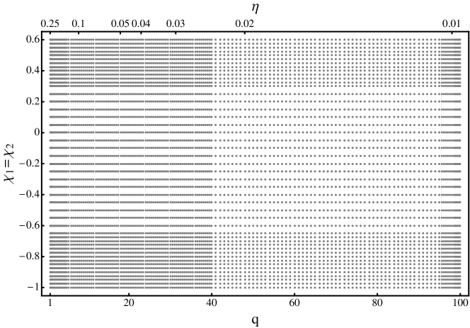
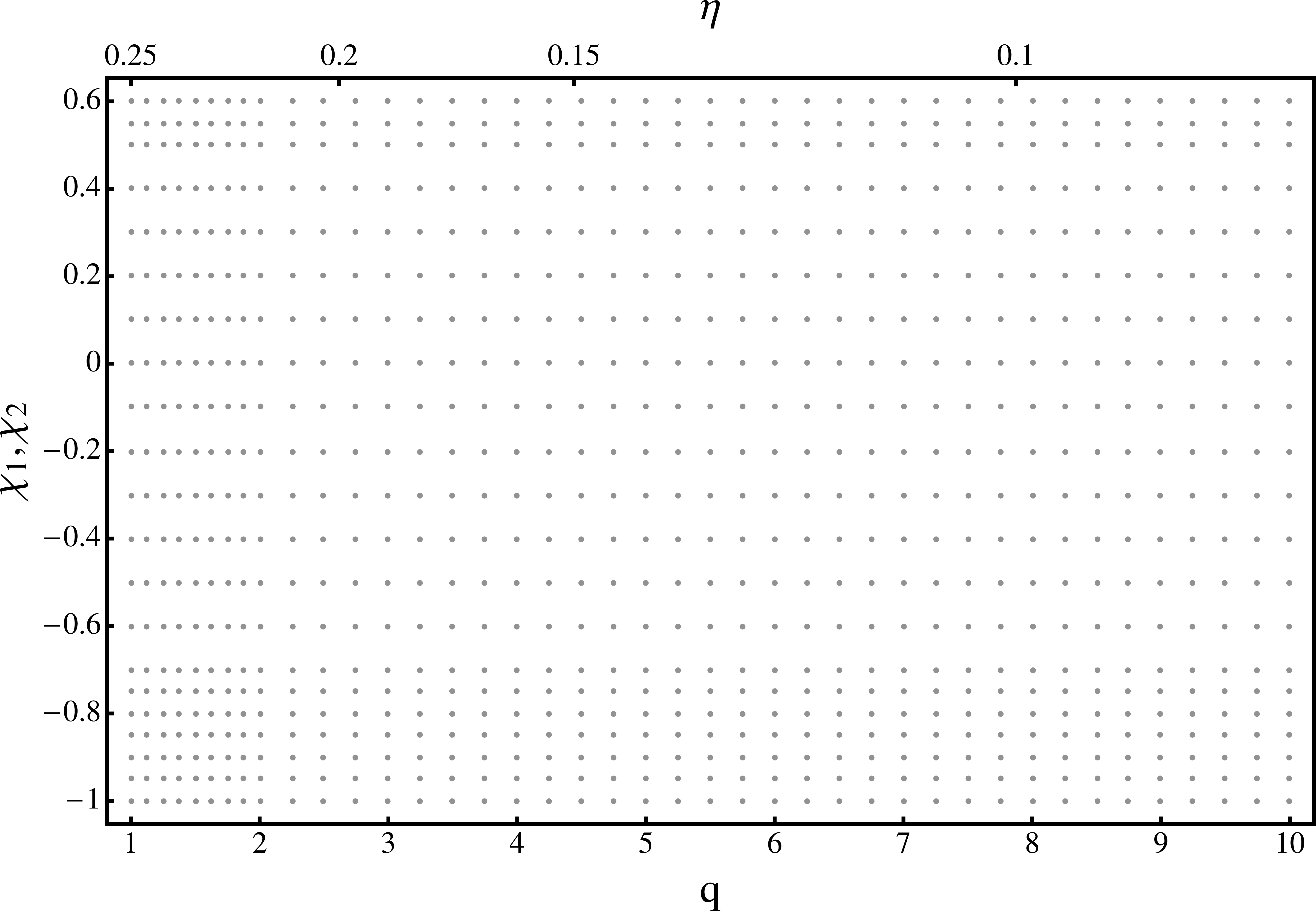
where and are one-dimensional sets covering the desired parameter range. For the equal-spin case I choose to cover the interval in mass-ratio and to cover the available extent in spins . The spacing in the mass-ratio and the spin is chosen in an uneven way to concentrate more points near the boundaries of the domain and at lower mass-ratios. Figure 2 shows how the parameter space was covered.
Next, I discuss how the frequency domain waveforms were calculated. The time-domain SEOBNRv1 waveforms are sampled at a rate of . In geometric units () this yields a time spacing of
| (4.2) |
The total mass is expressed in solar masses and is the geometrized solar mass in seconds. At we get which corresponds to a Nyquist frequency of .
At this time resolution, an equal-mass waveform long enough for a BNS system down to obtained from the LAL SEOBNRv1 code is given on about points and is about long in time. 444 I compute waveforms at (for equal-mass), but lower the starting frequency to Hz to obtain waveforms of sufficient length for BNS configurations, while keeping the full merger ringdown part.) The spacing in the frequency domain is
| (4.3) |
Combining this with the definition of the Nyquist frequency and the relation we have
| (4.4) |
With the above example, .
We taper the waveform with a Planck window [60] at both ends and zero-pad it by doubling the length of the waveform. Then we perform the FFT of the time-domain waveform and obtain data points at positive frequency. After separating the frequency domain waveform into its amplitude and phase part and unwrapping the phase we only need to keep a fraction of the number of points. We save about 500000 points to data files. To make the computation of the input waveforms more efficient, one only needs to make them long enough such that the mass of the smaller companion is at least that of a chosen physical cutoff, say . However, all waveforms need to be represented on the same grid for the SVD to make sense. Therefore, I hybridize the waveforms with TaylorF2 to make them of sufficient length in frequency. This is described in A.
The discrete amplitude and phase of each waveform in are treated separately. All waveforms are interpolated onto a frequency grid . A simple choice is an equidistant grid with gridpoints in the frequency interval . This is motivated by the starting frequency in geometric units for a BNS system at lower cutoff is . The interpolation error associated with this choice and the generation of more efficient sparse frequency grids are discussed in Section 5. The amplitudes are normalized using the norm induced by the discrete inner product . The waveforms are generated at a distance of Mpc with “face on” inclination. In Section 6 I will explain how the correct amplitude prefactor is restored. I subtract a linear fit from each of the hybrid phases in order to approximately factor out two degrees of freedom that have no physical significance. These correspond to time and phase shifts one maximizes over in the computation of the match between two waveforms.
5 Sparse frequency representation of waveforms
The goal of this section is to find a sparse set of frequency points on which one can represent the amplitude and phase functions of a frequency domain waveform to sufficient accuracy by using interpolation methods. I an algorithm based on the form of the spline interpolation error that can be used to obtain such a set of points and how it performs in terms of a parameter maximized inner product between (normalized) waveforms, the overlap or match, against the starting waveforms given on a fine equispaced grid.
A natural way of comparing two waveforms and is the scalar product
| (5.1) |
where is the one-sided power-spectral density of the detector noise. In this paper I use the expected design sensitivity of the Advanced LIGO detector [1, 61, 62]. The anticipated optimum sensitivity is given by the “zero-detuned high-power” noise curve [54]. We use a linear interpolation of this expected PSD and choose Hz, and kHz for the single spin model. For the double spin model the waveforms are generated for and Hz. denotes the Fourier transform of a time-domain waveform . The scalar product induces a norm . We maximize over time and phase shifts between the two waveforms and define the overlap (or match) as
| (5.2) |
where is the inverse Fourier transform. We often quote the mismatch instead.
Since the amplitude and the phase are typically fairly simple, smooth functions it should be possible to represent them as an interpolant on a sparse frequency grid. A priori it is not clear how to choose such a grid in an optimal way so that the errors in the computation of the overlap introduced by this approximation are below a desired threshold. We expect the interpolation error in the waveform phase to be the dominant source of error due to the way it appears in the overlap integral
| (5.3) |
Accumulating a significant dephasing over many GW cycles will cause the match to degrade more than a comparable level of error in the amplitude will.
Ideally it would be best to directly generate a grid based on minimizing the error in the overlap, i.e. the mismatch between the waveform on the equispaced grid and on the sparse grid. However, in practice pointwise error estimates are needed to find a grid without making assumptions on how the gridspacing should vary as a function of frequency. Starting iteratively from two endpoints, it is possible to compute the overlap of the spline interpolation of a current grid plus a new grid point taken from the base equispaced grid with the waveform on the full equispaced grid and chose to add the grid point that leads to the highest overlap. However, the overlap as a function of the phase error tends to threshold quickly and such a method turned out not to be well conditioned.
In Section 5.1 I discuss a method that chooses the gridspacing as a function of frequency such that the local spline interpolation error stays roughly constant. I interpolate amplitudes and phases using cubic splines over the set of chosen frequency points and start with a grid that only consists of the start and end frequency on which the waveforms are given. An alternative greedy method with the idea to successively add grid points at which the relative or absolute errors are highest is outlined in Section B. In practise I found the spline error method described in Section 5.1 to be more accurate and easier to use and I therefore chose it for the models described in this study.
The goal is to generate the smallest set of frequency points required for a given accuracy of the model. In practice one to two hundred points were sufficient for the models considered here. This leads to a substantial compression which makes the final model quite compact and also speeds up the generation of the model significantly since the rank of the basis matrices is then only a few hundred and the computation of the SVD of sparsely sampled waveform matrices takes on the order of a second which makes any performance advantage of the greedy basis algorithm over the SVD a moot point for this application.
5.1 Constant spline interpolation error (CSE) points
The idea for this method is guided by the form of the spline interpolation error. The error of a cubic spline interpolant of a function with derivatives given at the endpoints on a set of nodes with the largest gridspacing is [63]
| (5.4) |
where is the fourth derivative of . This bound makes it clear that in order to find a set of “good” nodes the functional form to be approximated needs to be taken into account. In practice I use cubic splines with a “not-a-knot” condition [64] at the endpoints rather than specifying the actual derivatives. This is the recommended condition for closing the system of equations if only the function values are known (i.e. in the absence of derivative information). The interpolation error of the “not-a-knot” spline is of the same order as the error given in Equation (5.4) and the precise error constant is not important in the following.
Before we think about generating sparse grids let us consider the error associated with the representation of the input waveforms on an equidistant grid. As described in Section 4 the equal-spin input waveforms we proposed to interpolate the amplitudes and phases onto a 10000 point equally-spaced frequency grid
| (5.5) |
Using this grid, the maximum relative error in the amplitude is about and the absolute error in the phase is less than for a equal-mass waveform starting at . In both cases the error is largest at the low frequency end and decreases very rapidly as the frequency increases. This grid is actually not sufficiently fine to guarantee very small errors down to the BNS regime. There the mismatch due to interpolation error is about . To push the phase error below for a BNS starting at would require about equispaced points. The sparse grids defined below are much more compact and also more accurate at low frequencies.
To generate a sparse frequency grid we demand that the gridspacing as a function of frequency is chosen such that the local spline interpolation error (i.e. we apply Equation (5.4) for every subset of 4 grid points) stays constant over the desired frequency range. Going back to Equation (5.4) we see that the gridspacing as a function of frequency has to be proportional to the reciprocal of the fourth root of the fourth derivative of the function to be approximated so that the error stays constant (if the equality were to hold). Given an appropriately chosen gridspacing function a grid can then be generated in a very straightforward manner where the spline interpolation error stays approximately constant. This is outlined in Algorithm 1.
Now I give examples on how to choose the gridspacing function: Assuming a simplified amplitude we find . In practice a linear dependence on frequency serves better to suppress amplitude error near the merger. For the phase we look at the dominant terms in the phase evolution of the TaylorF2 approximant for an equal-mass non-spinning binary: . The mass-ratio changes only the prefactors and the spins enter at higher PN order. With the help of a Taylor expansion we then find . In practice works well to keep the phase error balanced. The desired error threshold and, at the same time, the number of grid points can be set by adjusting the proportionality factor in .
For the single spin model I choose and . Starting at application of algorithm 1 yields 78 amplitude points and 200 phase frequency points. For the double spin model the waveforms are generated at a total mass of with an initial frequency of starting frequency of specified in LAL. It turns out that the lowest useable frequency is which is sufficient to fill the detector band down to .555Since this is a proof of principle paper, I choose to work with these double-spin waveforms; for practical models I intend to push this down to the cutoff demanded by aLIGO. There I choose and . This results in 95 amplitude points and 123 phase points. The number of points is less than for the single-spin model due to the higher total mass and starting frequency of the grid. These choices correspond to a maximum frequency domain amplitude error and phase error of .
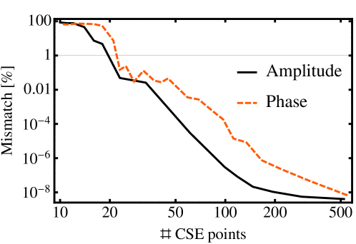
With this method it is very simple to adjust the resolution desired at low and high frequencies by changing the exponent of in the gridspacing function, so that one can guarantee good accuracy for a wide range of total masses. CSE points are by definition fairly evenly distributed in frequency and it is very fast and simple to generate them. Figure 3 shows how the mismatch decreases with the number of CSE frequency points. On the order of hundreds of points the interpolation error is already negligible for CSE points. The 100 to 200 points chosen above lead to both leading to a mismatch of about or less.
6 Building SVD-based reduced order models
This section deals with the singular value decomposition (SVD) and discusses some of its known properties as given in standard texts [65, 66] that are especially useful for reduced order modeling. We proceed in three steps: First, the SVD is used to obtain a compressed reduced basis representation of a collection of input waveforms. Second, projection coefficients of the input waveforms are calculated in terms of the reduced basis. Finally, a reduced order waveform model is assembled from the reduced basis and projection coefficients interpolated over the parameter space. Such a strategy has been pursued by Cannon et al for building time-domain reduced order models and working directly with the waveform strain [33, 32, 31].
The preprocessed amplitudes and phases are collected in the columns of separate waveform (or template) matrices ,
| (6.1) |
where is the total number of input waveforms, each waveform is given on a common grid of length and denotes the set of matrices with entries in . We may choose to represent the waveforms at a large number of frequency points so that . On the other hand, if the number of grid points has been reduced to a sparse set (see section 5) then we usually have .
Since we are dealing with a two- (or later when including both spins with a three-) dimensional parameter space we need to define a mapping that packs the waveforms on the rectangular parameter space grid into a single vector. First, we label a starting waveform at a specific mass-ratio and spin by the two-dimensional index pair , where , and . We then define a flat index which ranges from . We place the waveforms into successively as enumerated by this index. The two dimensional indices can be recovered as and .
We perform a singular value decomposition (SVD) [65, 66] of the waveform matrices
| (6.2) |
where and are orthogonal matrices. is a diagonal matrix made up from the singular values , and . The are the eigenvalues of . The and are the left and right singular vectors of , respectively. If has positive singular values then .
To obtain a reduced basis we can calculate a truncated SVD of the waveform matrices where we produce a rank-reduced approximation for a with the k-th partial sum of the outer-product expansion of the input matrix
| (6.3) |
and obtain a reduced set of basis vectors. We then have
| (6.4) |
i.e. is the best rank- approximation to in the Frobenius norm . The Frobenius norm can also be expressed by the vector 2-norm as , where denotes the th column of .
Note that the square of the Frobenius norm of the truncation error at rank
| (6.5) |
is equal to the sum of the squares of the 2-norms of the errors in each waveform amplitude or phase which make up the columns of . A useful estimate of the mean amplitude or phase error introduced by the approximation is the RMS norm of the truncation error .
The basis for the amplitude / phase space is given in the columns of the matrix if , if and a full rank basis is desired. If , then the information from the waveforms at grid points is contained in a basis of dimension . To compress the model one can define a reduced basis of rank
| (6.6) |
For any the columns of are an optimal orthonormal basis for the starting waveforms. We usually drop the label on the rank- reduced basis.
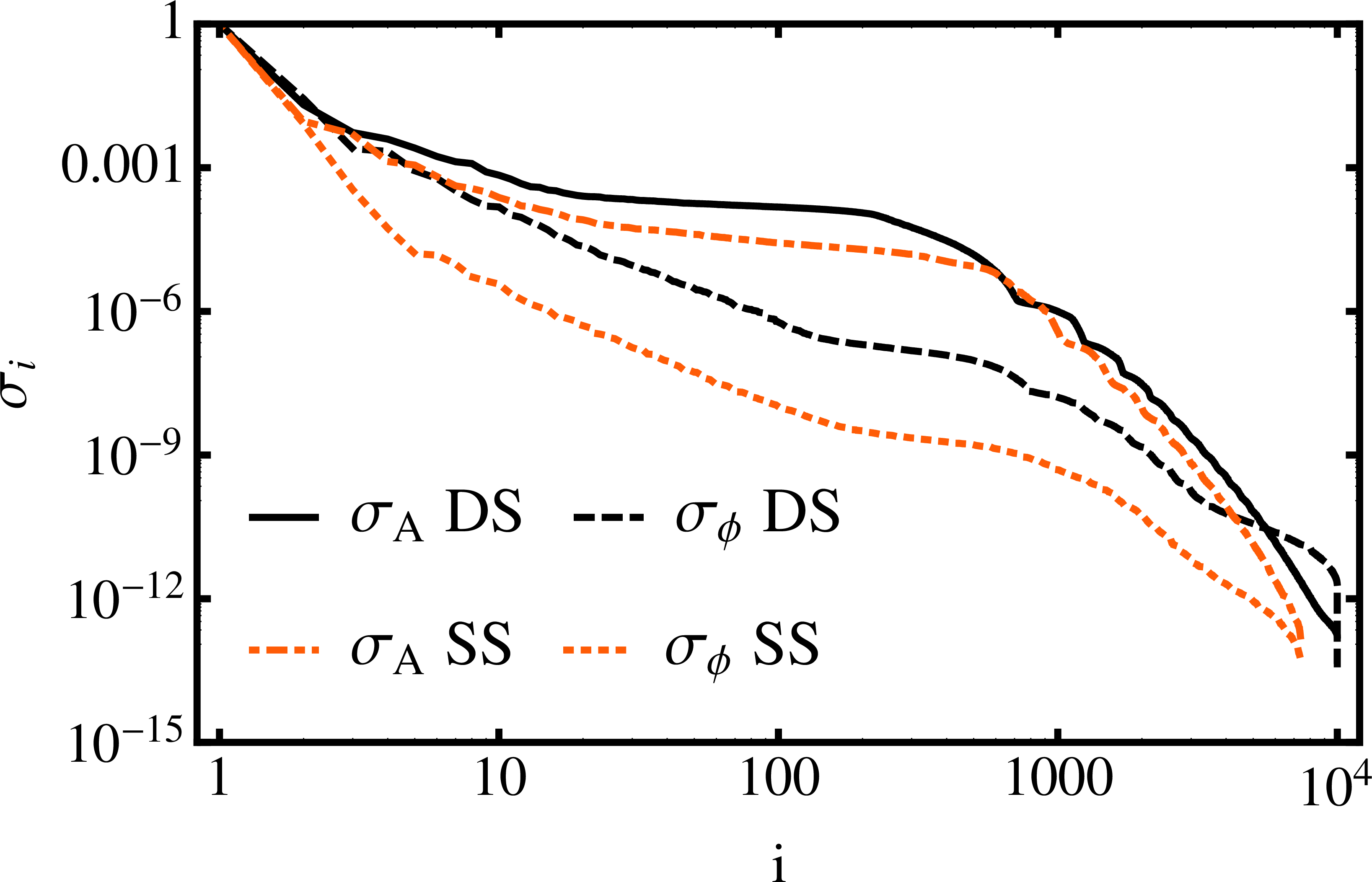
If the singular values decay sufficiently fast, then the truncation error is small, i.e. is a good compressed and fast approximation of . Fig. 4 illustrates that for the first few modes the singular values of the amplitude and phase waveform matrices fall off very rapidly, then settle down to a slower decay before an accelerated plunge beyond . The fact that the values are already reasonably small for on the order of a hundred motivates truncating the SVD after this many terms. Whether one thereby obtains an accurate compressed representation of the waveforms needs further investigation. In Section 9 and Figure 10 I will study the meaning of the truncation error in the Frobenius norm Equation (6.5) and compare it with the “mismatch” between waveforms introduced by this approximation.
Given the reduced bases and we compute projection coefficient vectors for any given input waveform amplitude or phase as follows
| (6.7) |
where we have dropped the amplitude or phase labels for brevity. We collect the projection coefficient vectors for all input waveforms in matrices and with entries
| (6.8) |
Comparing with Equation (6.2) we see that for a full-rank basis . It follows that the projection coefficient matrices are ordered in the same way as the individual waveforms in . To undo the packing of the waveforms in the matrices we just partition the linear index that enumerates the waveforms in and obtain a tensor
| (6.9) |
To complete the model we define the projection coefficient vectors at any location in the chosen parameter space by suitable interpolants for the amplitude and phase coefficient tensors . For each input waveform we have two corresponding -vectors of projection coefficients (for amplitude and phase) that are interpolated over the parameter space. This is discussed in Section 8. The frequency domain reduced order model is then given by
| (6.10) |
where denotes matrix multiplication, interpolates vectors in frequency on a suitable grid, and is an amplitude prefactor.
The amplitude normalization is restored as follows. We save the normalization factors that are applied to each amplitude before taking the SVD and compute an interpolant over the parameter space (using techniques discussed in Section 8). We restore the LAL amplitude scaling for a binary at arbitrary distance and optimal orientation by computing
| (6.11) |
where .
For optimal orientation the two polarisations of the dominant mode in the frequency domain are well approximated by
| (6.12) | ||||
| (6.13) |
since . We have conjugated the input waveforms so that the power is in the positive frequencies . The inclination of the binary only changes an overall amplitude factor for aligned-spin waveforms and the final expression for the polarizations is
| (6.14) | ||||
| (6.15) |
7 SVD and greedy reduced basis methods
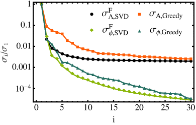
I give a brief comparison of the SVD and greedy basis [38, 40] methods. I contrast the falloff of singular values against the greedy error and show an example of how the greedy basis method picks configurations in the parameter space.
The greedy reduced basis algorithm (see e.g. Algorithm 1 in [38]) starts with a seed basis element and iteratively picks waveforms with the largest error in the orthogonal projection onto the basis from a set of input waveforms (also called the “training space”) and adds them to the basis. The basis elements are orthonormalized with a Gram-Schmidt algorithm.
Either the SVD or the greedy basis algorithm can be used to find a reduced orthonormal basis from a set of starting waveforms. Let be the number of waveforms given on gridpoints, assume , and let be the number of reduced basis functions desired. The greedy basis method has complexity (see e.g. [48]) as opposed to the SVD’s more costly and it can be trivially parallelized. For a full basis and the cost of the two methods is comparable. In contrast to the greedy basis method, parallel implementations of the SVD are readily available and easy to use. For a sparse frequency grid of about points, computing the SVD is very cheap, and takes about one second.
For both methods the reduced basis waveforms only resemble the physical behavior of frequency domain amplitudes and phases for the first basis function. Higher basis functions show corrections at finer scales and are oscillatory (see Figure 5). The falloff of the SVD truncation error Equation (6.5) and greedy errors is shown in Figure 6. It is worth noting that when using a truncated basis the SVD truncation error is, by construction, an average projection error. In contrast, the projection error associated with reduced basis elements chosen by the greedy algorithm minimizes local projection errors (see e.g. Algorithm 1 in [38]) and thus bounds the worst approximation error. This is consistent with the behavior shown in Figure 6.
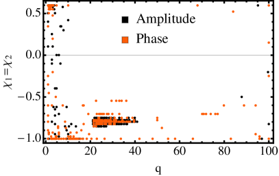
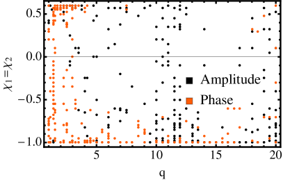
An advantage of the greedy algorithm is that it directly exposes which waveforms are picked from the space of input waveforms and then orthogonalized and promoted to basis vectors. Given a sufficiently dense set of waveforms in a subdomain of the physical parameter space this method provides valuable information on the variation of waveforms with the parameters. It can help identify problems in the underlying model when basis waveforms cluster in some region of the domain. Figure 7 shows the first 200 basis waveforms chosen from the single spin training space. Apart from clustering near the boundaries of the parameter space domain (similar to what was observed in [39]), basis waveforms are clumped together from and . This clustering shows up both for the independent amplitude and phase basis. This behavior is surprising as one would expect the waveforms to smoothly depend on mass-ratio and spin and may indicate that the source model contains unphysical artifacts, although here way beyond its calibration range .
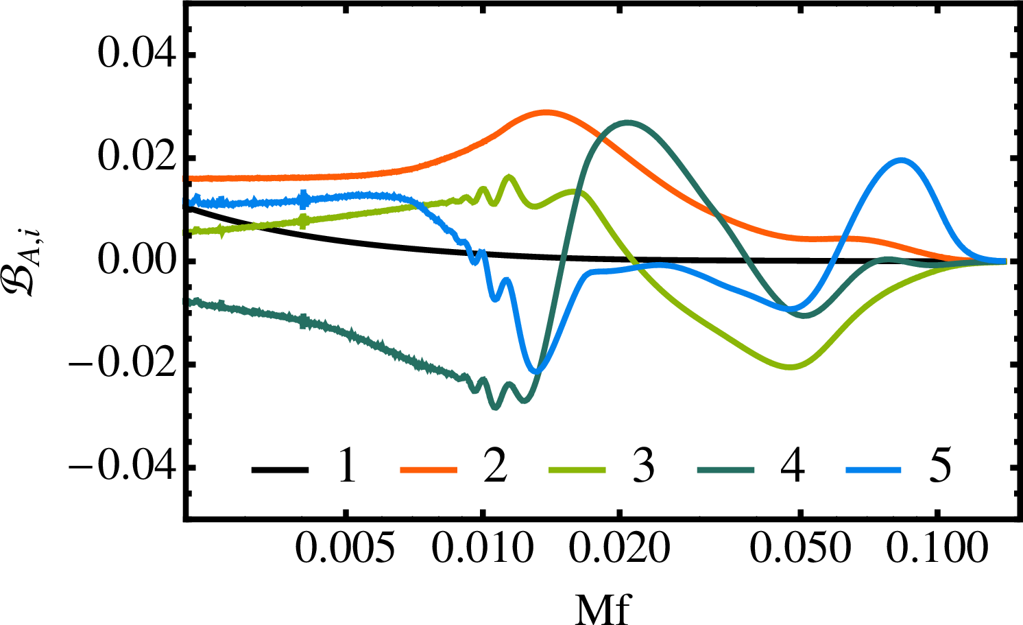
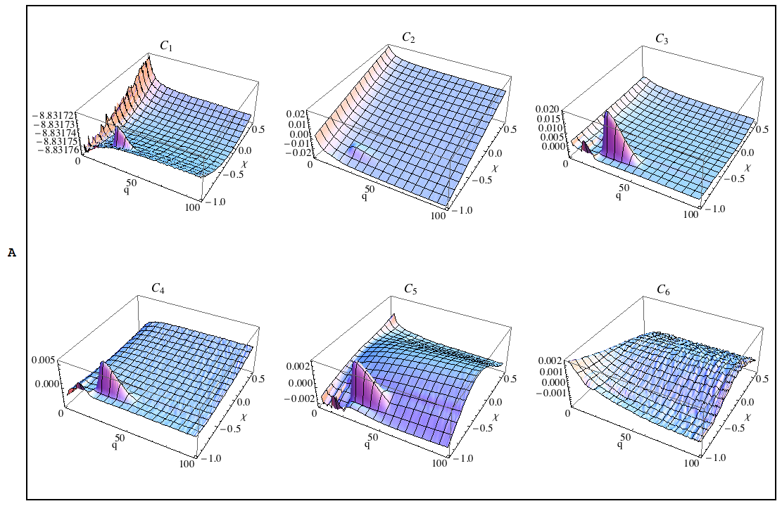
The clustering in Figure 7 and the peaks apparent in the amplitude coefficients in Figure 9 (see also Figure 13 for mismatches) turned out to be due to undersampling of the non-quasi-circular coefficients in the LAL implementation of SEOBNRv1 [67]. Since this study primarily deals with a proof of concept of building surrogates and since the regeneration of all input waveforms is very expensive the surrogate will not be rebuilt here. It is also instructive to see that reduced order modeling techniques can help in testing waveform models. Ultimately, I plan to build a surrogate model for the successor to SEOBNRv1 (SEOBNRv2) which covers the full spin range . This is the model that will be implemented in the LAL code.
If the source model is restricted to a range where it is deemed trustworthy (e.g. because it has been calibrated there) the method can show what the most physically important waveforms are and can provide clues where to perform NR simulations which can subsequently be used to improve current EOB and phenomenological waveform models. Given NR waveforms it is not possible to predict what the next most important NR waveform is that should be simulated without recourse to a trusted model.
8 Interpolation over the parameter space
There are many choices for creating interpolants of the projection coefficients over the parameter space. In the following I consider primarily tensor product spline interpolation, and briefly mention alternative methods. The discussion of the different interpolation methods assumes a two-dimensional parameter space; extension to a three-dimensional space is straightforward.
A natural way to interpolate the projection coefficients over the parameter space is to use a tensor product expansion. The tensor product interpolant of a scalar function on the Cartesian product of intervals is given simply in terms of the product of 1-dimensional basis functions ,
| (8.1) |
The points are taken from a rectangular parameter space grid with
| (8.2) |
and are the discrete expansion coefficients of in terms of the tensor product basis . We consider either cubic B-splines [64] or Chebyshev polynomials [68] as basis functions . Tensor product interpolants of vector valued functions are simply defined by component and generalizations to higher dimensions are straightforward.
One-dimensional cubic splines are piecewise polynomials of degree 3 with continuous first and second derivatives. Different choices are possible at the endpoints. A convenient condition that only requires the knowledge of the function values and no derivatives is the “not-a-knot” spline, where the first and last two spline pieces are taken to be the same polynomial. This is equivalent to the continuity of the third derivative at the second and at the penultimate grid point [69]. While the spline interpolant can be constructed directly by solving a system of linear equations from interpolatory and continuity conditions, it turns out to be convenient to introduce localized basis functions, B-splines, to facilitate generalizations.
Per default I use tensor product cubic splines as conveniently available in Mathematica 666Mathematica also provides tensor product Hermite interpolants where derivatives of the function need to be specified in addition to the function values. They are of comparable accuracy and speed to spline interpolants, but need a prescription for approximating derivatives if they are not available.. This method provides good accuracy, efficiency and does not require further adjustments if the variation of the coefficients is resolved by the grid. If the expansion coefficients and the B-splines are precomputed the evaluation cost of a -dimensional tensor product cubic spline interpolant goes as multiplications plus the cost of evaluating the non-vanishing B-splines at the desired physical parameter values.
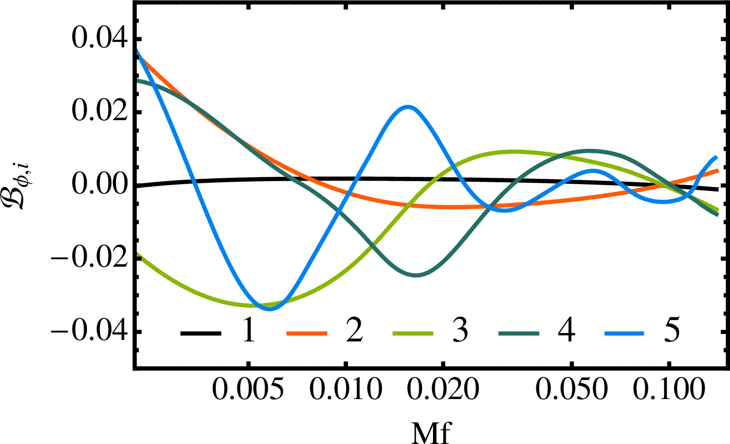
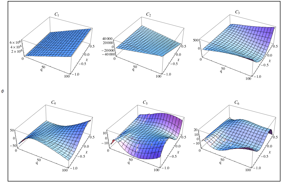
As can be seen in Figure 9 the first few projection coefficients for the phase are smooth functions. If the amplitudes are computed from the untreated input amplitudes, the coefficients turn out to be very rough near equal mass. Most likely this is due to noise from the long ODE integration and subsequent FFT that is apparent upon visual inspection. Smooth amplitude coefficients (as shown in Figure 9) can be obtained by fitting the inspiral part of the input amplitudes against a PN amplitude and combining the smooth PN fit with the unchanged data for higher frequencies. Here, the fit extended up to one quarter of the frequency of the innermost stable circular orbit (ISCO) of a test particle around a Schwarzschild black hole, , where . This change of the amplitudes has only a very small effect on the model, leading to mismatches of less than .
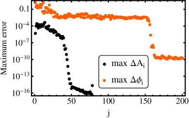
While it would be interesting to study the behavior of the B-spline interpolation error over the parameter space as a function of the density of input waveforms in order to optimize the choice of input configurations, such a study is beyond the scope of this paper. Instead, we can compare B-spline interpolants of the model against projection coefficients computed for a test amplitude or phase with randomly chosen mass-ratio and spin for each SVD mode . The difference is then a measure of the parameter space interpolation error in the model at parameters and can be computed for the amplitude and phase coefficients. A physically more meaningful error measure is the amplitude or phase error caused by the error in the projection coefficients in SVD mode ,
| (8.3) | ||||
| (8.4) |
where we take the maximum of the error over the discrete frequency points.
Figure 8 shows the maximum of this amplitude and phase error over a set of 1000 random test waveforms that are also used in Section 10. The errors are largest for the first few SVD modes and decrease gradually. Beyond for the amplitude and for the phase the errors fall off rapidly. This is consistent with the singular values reaching zero at these modes. This behavior is different from the more gradual falloff of the singular values seen in Figure 4 and is due to the representation of the amplitude and phase on a set of 78 and 200 sparse frequency points, respectively and allows for early truncation of the SVD expansion in the model.
In addition to tensor product spline interpolation I also tried tensor product Chebyshev [68] interpolation and radial basis functions (RBF) [70] which allow for general grids and scattered data. I found spline interpolation to be more efficient and since the evaluation speed of the model is more important than storage for most applications, I chose to use spline interpolation for the models build in this study. Similar to techniques for solving PDEs the division of the parameter space domain into a number of smaller subdomains may allow Chebyshev interpolation and radial basis functions help perform better. This technique would also allow the use of local refinement for tensor product expansions.
Even though the most important configurations in the parameter space (e.g.. as given by the greedy reduced basis method method [38, 40]) are distributed in an irregular way over the physical domain, a structured tensor product grid of waveforms is advantageous, because interpolation methods on tensor product grids are more accurate than methods designed for unstructured grids.
9 Other sources of errors
We have already come across the main sources of errors that arise in building surrogate models in the previous sections. Here I summarize these findings, study several further errors and draw some conclusions. The error due to a rank reduced SVD was pointed out in Section 6 and will be studied in more detail in this section. In Section 8 I mentioned the error due to interpolation of the projection coefficients over the parameter space, while in Section 5 I investigated the interpolation error in frequency due to the choice of a reduced set of grid points for the waveforms. Some of these error sources can be related to norms of amplitude and phase errors. Ultimately we seek a more physical interpretation and wish to study the impact of the individual errors in terms of the waveform mismatch.
9.1 SVD truncation error
One of the main ideas behind the approach pursued in this paper is a natural splitting of the frequency domain waveform into amplitude and phase and their representation by separate bases. These functions are nonoscillatory and “simpler” than the real and imaginary part of the strain and thus we expect to be able to find a more efficient compressed representation. Moreover, we can exploit additional freedom in finding optimal approximations if we treat amplitudes and phases completely separately. Unsurprisingly, we then found in Section 5 that the amplitude requires less frequency points than the phase in terms of a desired mismatch error due to interpolation. A disadvantage of performing this separation is that there is no direct relation between the singular values and the match. Such relations have been pointed out in the literature when the amplitude and phase were treated jointly and I address them briefly here.
Cannon et al [33] derive a relation between the singular values and the fractional SNR loss. They work directly with the complex (whitened) time-domain waveform. Field et al [38] give a relation between the greedy error of the reduced basis and the white-noise time-domain inner product between a waveform and its orthogonal projection onto the span of the basis. Such relations do not directly allow the computation of the detector noise weighted mismatch for a range of system masses. Since these relations are not applicable in the approach pursued in this paper I compute the mismatch numerically.
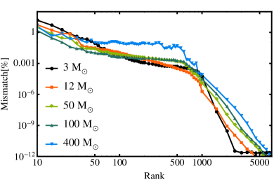
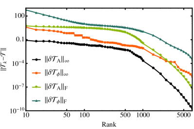
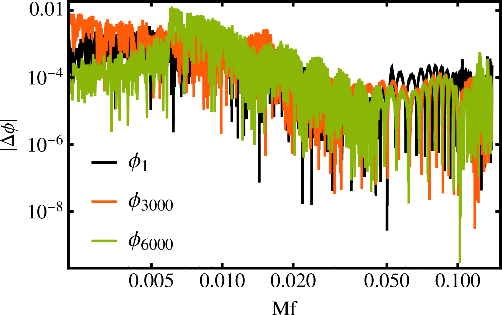
In Figure 10 I show the decay of the SVD truncation error with rank for the single spin waveforms. The error is quantified both by the mismatch of the full model against a rank model (top left) and the or Frobenius norm777 Note that since the Frobenius norm yields an average -norm of the waveform error, it can grossly overestimate the maximum phase or amplitude error. The and vector norms are related via the inequality , where . of the error in the waveform matrix (top right). In practise it is best to adjust so that the mismatch is smaller than desired. Except for very high total mass the mismatch due to SVD truncation is near for of the order of a few hundred. There, the Frobenius norm of the starting phases is on the order of ten while the norm is near . The bottom panel of Figure 10 gives an example of what the SVD truncation error looks like in terms of amplitude and phase error for selected waveforms. Both errors are highly oscillatory but their overall size is useful to remember and compare against, for instance, the amplitude and phase errors resulting from interpolation in frequency.
A final remark on a peculiar feature of SVD-based models with separated bases for amplitude and phase is in order. The SVD employs the Euclidean inner product to orthogonalize the basis functions. While this makes sense for the amplitude this is somewhat “unnatural” for the phase, as it enters the overlap in a complex exponential. Thus, the Euclidean inner product does not take into account that only the phase difference appears in the overlap.
9.2 Further sources of error
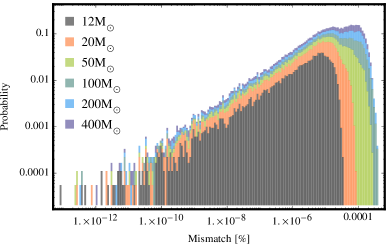
The interpolation error over the parameter space was mentioned in Section 8. It arises due to the interpolation of the projection coefficients . This error depends on smoothness of the projection coefficients (see Figure 9) and the inherent accuracy of the chosen interpolation method. I compared different types of interpolants and settled for the robust choice of tensor product cubic splines. Since the smoothness of the coefficients is a priori unknown the interpolation error can only be computed by investigating the faithfulness of a given ROM model against waveforms that were not used in the construction of the model. Such a study with a set of waveforms at random locations in the model domain is carried out in Section 10 and Section 11. The mismatch error for the single spin model is shown in Figure 12 and Figure 11. The fidelity of the double spin model is tested in Figure 19. The mismatch is below for the double-spin model, but up to for the single-spin model which spans a vast range in the mass-ratio and encounters artifacts from the SEOBNRv1 source model.
An additional error source for the single-spin model is hybridization error. For the single-spin model I intended to extend the model into the binary neutron star domain. Due to the very high cost of generating SEOBNRv1 waveforms at these total masses I resorted to hybridization with the TaylorF2 approximant (see A for details). The TaylorF2-hybrids have a mismatch less than with SEOBNRv1 waveforms that cover the whole detector band at mass and Hz lower frequency cutoff. This error can be reduced further by producing longer waveforms and hybridizing at lower frequencies or can be avoided altogether if one is willing to pay the price for significantly more expensive waveform generation at higher mass-ratios.
Inaccuracies in the computation of the overlap: While not a problem of the model I caution the reader about a technical problem that appears in the computation of the overlap. In the construction of the models I subtracted a linear frequency fit from the input phases. This operation does not alter the physical content in the phase and is in principle neutralized by the maximization of time and phase shifts that is performed in the computation of the overlap. However, proper maximization over time-shifts requires a very fine frequency resolution in the presence of large linear dephasing between two waveforms. The models tend to have a very different phase evolution than SEOBNRv1 waveforms that were generated afterwards to test the model and the models may appear more unfaithful than they are. The remedy for this technical difficulty is either to subtract a linear fit from the phase difference of the waveforms in the computation of the overlap or to use substantial zero-padding. Zero-padding factors of up to 100 control this error sufficiently by providing a fine sinc interpolation (see e.g. [71]) of the complex SNR which allows accurate maximization over time shifts.
Initially I built ROM models from input waveforms on a fine equally spaced grid and employed SVD rank truncation to make the model more compact. There, I started with waveform matrices with a comparable number of grid points and number of waveforms . If the waveforms are linearly independent, . Later on I constructed ROM models in a different way: I first interpolated the input amplitudes and phases onto a set of sparse frequency points and then performed the SVD. In that case and the rank of the waveform matrix is now . This leads to a loss of information and an associated error. I will refer to it as the “rank-reduction” error that stems from using fewer frequency points than input waveforms in the SVD. In the absence of SVD truncation the square basis matrix has the same rank as the waveform matrix that I feed into the SVD. The error is due to the approximation of the input waveforms in the waveform matrix by SVD modes. If I kept the full matrix times the singular values I could reconstruct the full waveform matrix (except for numerical errors in the computation of the SVD). However I only keep a smaller set of projection coefficients . With this setup further SVD truncation at a lower rank is less useful and does not lead to significant further compression. An example of this “rank-reduction” error is discussed in Section 11 and Figure 19.
To summarize, in practice I build ROM models by first generating a set of sparse frequency points for the amplitude and phase, interpolating the starting waveforms onto those sets, performing a full SVD of the waveform matrices and finally interpolating over the parameter space. The errors introduced by the individual approximations combine in complicated and nonlinear ways. Even though it does not seem to be possible to predict the fidelity of the final ROM model, one can check its faithfulness explicitly by computing matches against an independent set of randomly generated waveforms (see Section 10 and Section 11).
In the models constructed for this paper the interpolation of projection coefficients over the parameter space turned out to be the dominant source of error (see Section 10 and Section 11). To reduce this error a finer spacing of input waveforms in regions where the coefficients are not sufficiently smooth is required. How much refinement is needed can only be explored iteratively and is evidently a very costly endeavor. Furthermore one has to be aware that while the fidelity of a model can be increased by adding more input waveforms, its evaluation speed will be reduced and storage requirements will be increased.
10 Results for single-spin models
Here I summarize results for models using a single-spin approximation and are built from equal-spin waveforms similar to the approach used in phenomenological models for aligned-spin binaries [51, 15, 16, 52]. Individual error sources are discussed at length in Section 9. In this section I focus on faithfulness results for single-spin models, that is, the match between a given SEOBNRv1 waveform and the surrogate model using the same parameters. Matches were computed with a frequency spacing of .
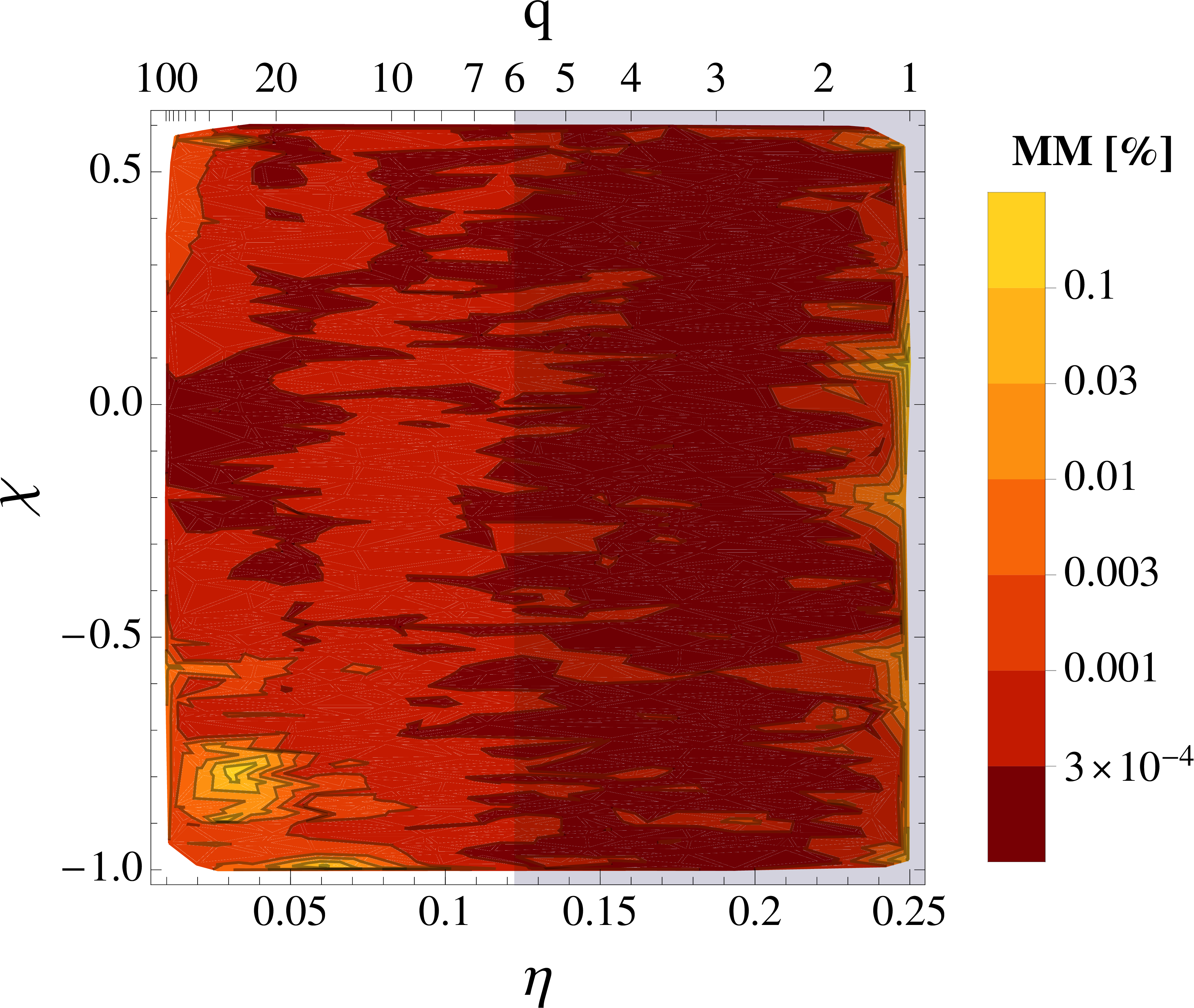
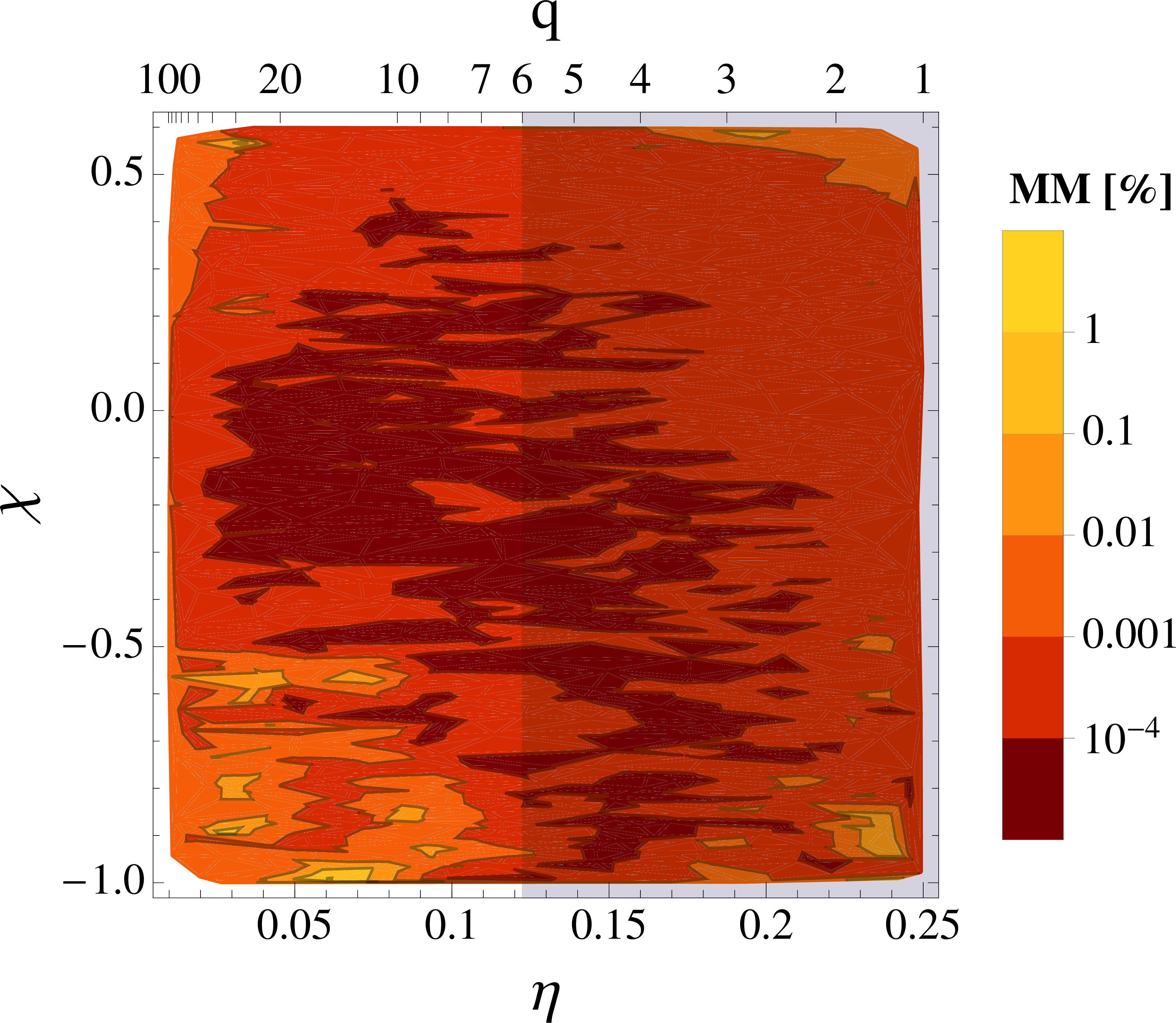
In Figure 11 the mismatch between a full CSE SVD model and 1000 equal-spin waveforms randomly distributed in the symmetric mass-ratio and is displayed. The left panel shows a contour plot of the mismatch at fixed mass . The mismatch rises slightly towards equal mass. This is due to phase error at low frequencies. The mismatch at is below for all values of and . More interesting are localized “islands” where the mismatch is higher than the ambient value. The dominant island in the left panel is near and . These do not look as serious as one would expect from Figure 9. The matches are worse there because the model does not capture the behavior of SEOBNRv1 very accurately in this region; but one would expect the matches to be much worse if the model’s amplitude and phase projection coefficients were very smooth there, contrary to the peaks visible in Figure 9.
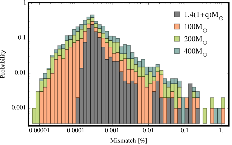
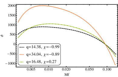
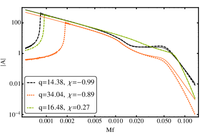
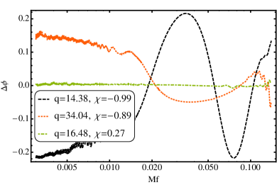
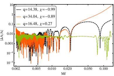
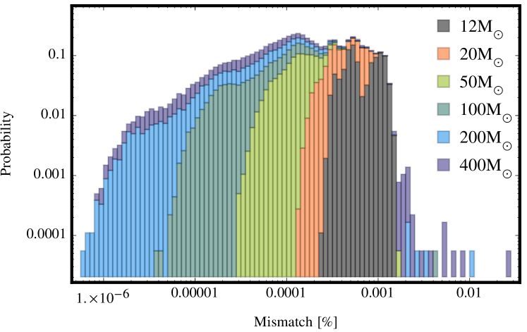
The right panel of Figure 11 plots the mismatch at a total mass of . There we see multiple islands at high negative spin. Isolated configurations (compare with the histogram in Figure 12) have mismatches above . These are located at , and , . Except for these two configurations the mismatch is below . These configurations are close to “clusters” in the greedy reduced basis (see Figure 7) and are due to undersampling of NQCs in the SEOBNRv1 LAL code in these parameter space regions. The phase error for these configurations is shown in Figure 13. As can be seen from Figure 13 the phase and amplitude error for these configurations is nonlinear at fairly high frequencies. Figure 12 shows histograms of mismatches against the CSE single-spin ROM model for the same random configurations as in Figure 11. In addition histograms are also shown for total masses and .
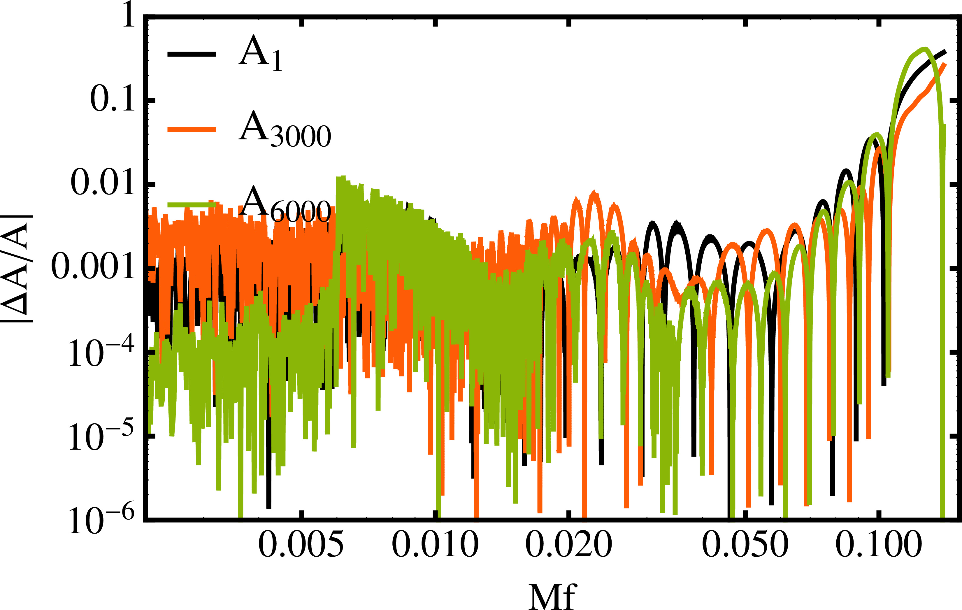
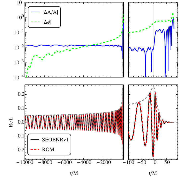
To corroborate the fact that the ROM model is of high fidelity beyond high faithfulness I show a time-domain comparison in Figure 14. The inverse FFT of the ROM model is compared against an SEOBNRv1 waveform. The upper panel shows the amplitude and phase errors. The amplitude error is about right until the amplitude maximum, then rises to and more in the final stages of the ringdown. Similarly, the phase error (with alignment at ) is below rad until shortly before the merger, rises to rad through merger and peaks at rad well into the ringdown. The bottom panel plots the real part of the strain waveform. The disagreement in the waveform is barely visible near the merger. The accuracy of the ROM model is comparable to amplitude and phase errors quoted for the SEOBNRv1 model in Section 3. The mismatch at is smaller than . The frequency domain phase error (see Figure 15) is below rad from ( Hz lower cutoff at ) to . The frequency domain amplitude error is below . The phase error in the Fourier domain should not be confused with the phase error in the time-domain, which is a more familiar quantity.


11 Results for double spin models
So far the discussion has mainly focussed on the single spin model. Since the source SEOBNRv1 model allows for two independent spin components I have also constructed a double spin model in a more restricted parameter space region. Here I discuss some of the choices made for that model and assess its fidelity.
Due to the increase in dimensionality and the indications that the source model may not be correct at higher mass-ratios (see the clustering of waveforms in Figure 7) I choose to restrict the extent of the parameter space covered to . While this goes beyond the calibration domain of SEOBNRv1, this choice is motivated by the model’s mismatch against a non-spinning NR waveform in the NRAR catalog.
I pick a spacing of and with additional waveforms near equal-mass and near the spin boundaries and . In total I use waveforms on a tensor product (rectangular) grid as shown in Figure 16. The waveforms are sampled at a rate of and a specified initial frequency of for the LAL code. Due to the high computational cost I generate these waveforms at a higher total mass of for all mass-ratios considered here in order to avoid hybridization. This eliminates the hybridization error which would be significantly larger at than for BNS waveforms. With a generation time of several minutes this is feasible at this higher total mass. The lowest usable frequency in frequency domain waveforms is . This is sufficient to fill the detector band down to about . For practical models I will generate waveforms that reach the lower cutoff required for aLIGO, but for the proof of principle models discussed here the results displayed use a lower cutoff of Hz.
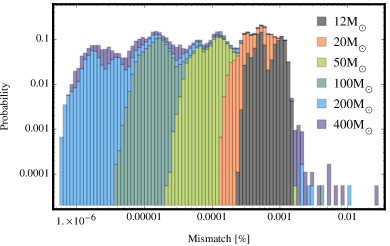
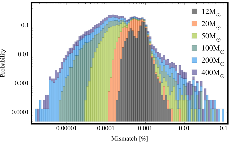
I interpolate the waveforms obtained from the FFT of time-domain SEOBNRv1 waveforms onto a constant spline interpolation error (CSE) grid as discussed in Section 5.1. I have already investigated the error introduced by this interpolation in frequency in Figure 17, but I study it here again for all input waveforms. First I show the faithfulness of the CSE model against the set of input waveforms in Figure 17. The mismatch is below for almost all waveforms and total masses considered. It arises from two individual error sources: (a) the mismatch induced by the interpolation of each input waveform onto the CSE amplitude and phase points in frequency and (b) the “rank-reduction” error that stems from using fewer frequency points than input waveforms in the SVD. These errors are investigated individually in Figure 18. We see that the frequency interpolation error (left panel) can be as high as , while the rank-reduction error (right panel) is below for all total masses considered. This is consistent with the total mismatch shown in Figure 17 and the bound on the combination of mismatches given in Equation (12.1). This shows that the mismatch due to frequency interpolation is the larger of these two error sources.
Finally, I test how faithful the CSE double-spin model is against a set of about SEOBNRv1 waveforms which are generated at random points in the parameter domain of the model. As shown in Figure 19 the mismatch for the “zero-detuned high-power” aLIGO noisecurve is better than up to , better than up to and below beyond . The mismatch is comparable for the “early aLIGO” [72] noisecurve, better at low total masses and slightly worse at high total masses. Comparing with Figure 17 we see that interpolation error over the parameter space is the dominant error source in the final model. The highest mismatches arise predominantly for configurations near mass-ratio and near extremal negative spin on the larger BH, i.e. near two of the boundaries of the parameter domain.
12 Discussion
I give a brief comparison of SVD and greedy reduced basis methods, summarize the accuracy, performance, speed and storage requirements of the SEOBNRv1 reduced order models discussed in this paper. Finally I address how the techniques presented here can be extended to build models for GWs from generic binaries.
A matter of practical importance are the storage requirements of reduced order models. As a point of reference we define as the starting size the set of input waveforms on a point frequency grid, which is about double precision floating point numbers for the double-spin input set considered here. The final size of the reduced basis for the double-spin CSE model is floating point numbers. However the model also includes projection matrices for all input waveforms. This is the dominant contribution to storage size. The overall size of the double-spin CSE model is about . Compared to the size in bytes of the starting waveforms the information has been compressed by roughly a factor of . The total storage size is determined by the number of sparse frequency points (this determines the size of the basis matrices) and the number of input waveforms covering the parameter space (this sets the size of the projection coefficients). To reduce the data required for the model, the number of input waveforms could be reduced. This would lead to an increase in the interpolation error over the parameter space which is already the dominant ROM error. An alternative to achieve higher compression is to use fits to the projection coefficients instead of interpolation. Fits require in general a bit of tweaking and may introduce further errors, while interpolation is automatic and robust.
Looking back at Equation (6.10) the evaluation cost of the ROM consists of evaluating the tensor product interpolants of the projection coefficients , matrix multiplication between the reduced bases and the , and the construction and evaluation of the one-dimensional cubic splines for the desired number of frequency points. For full reduced bases , the total cost goes as , where is the number of sparse frequency points, the number of input waveforms and the number of model evaluations in frequency. The solution of the linear systems for constructing the tensor product interpolants over the parameter space can be cached; therefore the associated cost is not included here.
Let us mention that we could have used a rank reduced SVD to make models based on a sparse set of frequency points (such as CSE points) still more compact. The size of the projection coefficients and the reduced basis matrix decreases when truncating the SVD at rank . However, since the number of frequency points was already chosen to be small, there may not be much further leeway for compression without significant loss of fidelity. Therefore the SVD truncation technique is more useful when working with a large set of frequency points.
As discussed in Section 3 the SEOBNRv1 model was found to be faithful to for total masses between and using the aLIGO “zero-detuned high-power” noisecurve. I showed in Section 11 that the double-spin surrogate model is faithful to SEOBNRv1 to about for total masses above and for or lower. Clearly the ROM error is much smaller than the uncertainty in the original model. We can then estimate that the mismatch between “true” NR waveforms (against which SEOBNRv1 has been compared) and the surrogate model presented here is better than at high total masses and better than below by using the triangle inequality [73]
| (12.1) |
Note that the actual total mismatch may be much lower than the bound obtained from this inequality. Since ROM error is much smaller than the uncertainty in the original model it is not necessary to improve the surrogate model even more.
An important practical question for waveform models is how low the mismatch must be so that PE calculations are not compromised. This can be answered by requiring that the error of the model against a set noise level be indistinguishable [74, 73] for a detector. For the waveform error to be smaller than unity the mismatch needs to satisfy . Assuming that the SEOBNRv1 is “true” we see then that the double-spin model with its modeling mismatch of is sufficiently accurate for PE up to SNR for total masses above and up to SNR for lower total masses. This is comparable or better than the mismatch spacing of templates used in the SVD-based model tested in [30] for PE applications. It should be noted that the above criterion on the mismatch is a sufficient but not a necessary criterion and it can be too stringent as shown in [23] for the nonspinning EOBNRv2 model [22].
This paper presents a general prescription for building SVD-based frequency domain models for GWs from aligned spin binaries and the first practical reduced order model of SEOBNRv1 that can be used for GW data analysis. The ROM model can be used for searches, but also for parameter estimation where such a model is urgently needed to enable in-depth studies that have so far not been possible due to the prohibitive cost of generating SEOBNRv1 waveforms on the fly. A reduced order model for SEOBNRv2 will be made available in the publicly accessible LAL software package [53].
The modeling techniques discussed here can be applied to any aligned spin model. Producing a model for the followup SEOBNR model [57] would be useful in order to assess the improvements over the parameter space, lift the restriction on aligned spins that is present in the current model and to provide a model with even higher fidelity. The techniques can be extended in a straightforward way to create reduced order models including higher modes.
Models of GWs from precessing binaries can be built either on a mode-by-mode basis, or, following the way recent models have been constructed, by twisting up (using Wigner rotations) aligned spin waveforms with time- or frequency-dependent angle functions that describe the motion of the orbital plane. Thus, in addition to the aligned spin waveform, the angle functions will need to be modeled in an efficient manner [75, 76, 77]. Modeling the full precessing parameter space without an (approximate) mapping between aligned spin and precessing waveforms is a daunting task and due to the lack of a sufficient number of NR waveforms or IMR models that take this approach it is only applicable in the PN regime. There, a reduced order model could shed light on degeneracies that are suppressed by the decomposition of the space using Wigner rotations.
13 Acknowledgements
It is a pleasure to thank M. Hannam, F. Ohme, A. Buonanno, M. Tiglio, S. Field, C. Galley, R. Smith, C. Hanna, S. Husa, P. Cañizares-Martinez, B. Sathyaprakash, S. Fairhurst, P. Sutton for useful discussions and comments. I thank the anonymous referees for their detailed comments and suggestions which helped to improve the presentation of the paper. This work has made use of Mathematica packages written by S. Husa, M. Hannam, F. Ohme and myself. I acknowledge support by Science and Technology Facilities Council grants ST/I001085/1 and ST/L000962/1.
Appendix A Hybridization
SEOBNRv1 waveforms are very expensive to generate, in particular, when the total mass becomes close to that of a neutron star. As one goes to higher mass-ratios the lowest meaningful system mass is going to be higher than times the mass of a neutron star. To ease the computational burden it makes sense to generate waveforms at mass-ratio at these total masses. However, in order to build a model and used reduced basis techniques such as the SVD, all waveforms have to be defined on the same frequency grid. To achieve this we create frequency domain TaylorF2 hybrids and follow a procedure outlined in [51, 16].
The calculation of SEOBNRv1 frequency domain waveforms was already described in Section 4. The matching procedure aligns and by a least squares fit over a frequency fitting interval . We then determine the matching frequency at which the NR and EOB phases coincide by a root-finding algorithm. The PN and EOB amplitudes are aligned separately without any freedom to adjust parameters. The hybridization interval for amplitude and phase is chosen as follows
| (1.1) | ||||
| (1.2) |
where is the lowest usable frequency for each waveform. This quantity rises with the mass-ratio.
The impact of hybridization on the ROMs is very small since the added low frequency content is only needed to perform the SVD of the waveform matrix and is not going to be in the detector frequency band when the system mass is chosen to be higher than times the mass of a neutron star. In that sense any smooth low frequency extension could be used, even if it were unphysical.
Appendix B Greedy frequency points
This section discusses an alternative algorithm for producing sparse frequency points. The basic idea is to successively add grid points at which the relative or absolute errors are highest to a skeleton grid.
Separate greedy algorithms (see 2 and 3) are used to find a set of amplitude or phase points . Let / be a subset of input waveform amplitudes / phases that are spline interpolated over the frequency grid . The subsets / can be chosen as the first, say 150, greedy basis configurations (as obtained from Algorithm 1 in [38]). This will cover the major variations in the functions and so ensure that all waveforms will be interpolated to high accuracy.
We use different error measures for amplitudes and phases. We discuss the algorithm for the amplitude first and then point out the differences in the algorithm used for the phases. We start with a skeleton grid consisting of just the endpoints. In each iteration a new amplitude point is found in 2 by first computing relative error vectors and their norms for each amplitude in the set . Then we find the index of the error vector with the largest error norm and the grid point at which the error is largest in that is not yet part of our current grid. We iterate until a desired error tolerance has been obtained. To generate the phase points in 3 we use a combination of relative and absolute errors, subtract a linear fit from each phase difference to remove the influence of time and phase shifts which are of no interest. These algorithms are inspired by the empirical interpolation method [37, 38, 48] in the fact that the point with the largest pointwise error is promoted to be a new grid point.
One can use e.g. cubic spline interpolation for its simplicity and robustness, although high order polynomial interpolation can be used as well. In applying this method to subsets of SEOBNRv1 input waveforms considered in this paper I found that the error falls off steeply for the first about 50 points, but then tends to threshold, especially for the amplitude. This surprising flattening would benefit from future study. The error becomes smoother as the size of the subsets / is increased. Lower errors can be obtained for smaller subsets.
References
References
- [1] Abbott B et al. (LIGO Scientific) 2009 Rept. Prog. Phys. 72 076901 (arXiv:0711.3041)
- [2] Accadia T et al. (Virgo Collaboration) 2012 J. Instrum. 7 3012
- [3] Grote H (for the LIGO Scientific Collaboration) 2010 Class. Quantum Grav. 27 084003
- [4] Harry G M et al. (LIGO Scientific Collaboration) 2010 Class.Quant.Grav. 27 084006
- [5] Acernese F et al. (The Virgo Collaboration) 2009 Advanced Virgo Baseline Design [Virgo Techincal Document VIR-0027A-09]
- [6] Abadie J et al. (LIGO Scientific) 2010 Class. Quant. Grav. 27 173001 (arXiv:1003.2480)
- [7] Aasi J et al. (LIGO Scientific Collaboration, Virgo Collaboration) 2013 (arXiv:1304.0670)
- [8] Sathyaprakash B and Schutz B 2009 Living Rev.Rel. 12 2 (arXiv:http://www.livingreviews.org/lrr-2009-2)
- [9] Somiya K (for the KAGRA Collaboration) 2012 Class. Quantum Grav. 29 124007 (arXiv:1111.7185)
- [10] Allen B, Anderson W G, Brady P R, Brown D A and Creighton J D 2012 Phys.Rev. D85 122006 (arXiv:gr-qc/0509116)
- [11] Blanchet L 2014 Living Rev.Rel. 17 2 (arXiv:1310.1528)
- [12] Buonanno A, Iyer B, Ochsner E, Pan Y and Sathyaprakash B S 2009 Phys. Rev. D80 084043 (arXiv:0907.0700)
- [13] Brown D A, Kumar P and Nitz A H 2013 Phys. Rev. D 87 082004 (arXiv:1211.6184)
- [14] Centrella J, Baker J G, Kelly B J and van Meter J R 2010 Rev.Mod.Phys. 82 3069 (arXiv:1010.5260)
- [15] Ajith P et al. 2011 Phys. Rev. Lett. 106 241101 (arXiv:0909.2867)
- [16] Santamaria L et al. 2010 Phys. Rev. D82 064016 (arXiv:1005.3306)
- [17] Buonanno A and Damour T 1999 Phys. Rev. D59 084006 (arXiv:gr-qc/9811091)
- [18] Buonanno A and Damour T 2000 Phys. Rev. D62 064015
- [19] Damour T, Jaranowski P and Schaefer G 2000 Phys.Rev. D62 084011 (arXiv:gr-qc/0005034)
- [20] Damour T 2001 Phys.Rev. D64 124013 (arXiv:gr-qc/0103018)
- [21] Damour T, Iyer B R and Nagar A 2009 Phys.Rev. D79 064004 (arXiv:0811.2069)
- [22] Pan Y, Buonanno A, Boyle M, Buchman L T, Kidder L E et al. 2011 Phys.Rev. D84 124052 (arXiv:1106.1021)
- [23] Littenberg T B, Baker J G, Buonanno A and Kelly B J 2013 Phys.Rev. D87 104003 (arXiv:1210.0893)
- [24] Aasi J et al. (LIGO Scientific Collaboration, Virgo Collaboration, NINJA-2 Collaboration) 2014 Class.Quant.Grav. 31 115004 (arXiv:1401.0939)
- [25] Taracchini A, Pan Y, Buonanno A, Barausse E, Boyle M et al. 2012 Phys.Rev. D86 024011 (arXiv:1202.0790)
- [26] Harry I W, Allen B and Sathyaprakash B 2009 Phys.Rev. D80 104014 (arXiv:0908.2090)
- [27] Manca G M and Vallisneri M 2010 Phys.Rev. D81 024004 (arXiv:0909.0563)
- [28] Ajith P, Fotopoulos N, Privitera S, Neunzert A and Weinstein A 2014 Phys.Rev. D89 084041 (arXiv:1210.6666)
- [29] Brown D A, Harry I, Lundgren A and Nitz A H 2012 Phys.Rev. D86 084017 (arXiv:1207.6406)
- [30] Smith R, Cannon K, Hanna C, Keppel D and Mandel I 2012 (arXiv:1211.1254)
- [31] Cannon K, Hanna C and Keppel D 2012 Phys.Rev. D85 081504 (arXiv:1108.5618)
- [32] Cannon K, Hanna C and Keppel D 2011 Phys.Rev. D84 084003 (arXiv:1101.4939)
- [33] Cannon K, Chapman A, Hanna C, Keppel D, Searle A C et al. 2010 Phys.Rev. D82 044025 (arXiv:1005.0012)
- [34] Cannon K, Emberson J, Hanna C, Keppel D and Pfeiffer H 2013 Phys.Rev. D87 044008 (arXiv:1211.7095)
- [35] Cannon K, Cariou R, Chapman A, Crispin-Ortuzar M, Fotopoulos N, Frei M, Hanna C, Kara E, Keppel D, Liao L, Privitera S, Searle A, Singer L and Weinstein A 2012 The Astrophysical Journal 748 136 URL http://stacks.iop.org/0004-637X/748/i=2/a=136
- [36] Privitera S, Mohapatra S R P, Ajith P, Cannon K, Fotopoulos N, Frei M A, Hanna C, Weinstein A J and Whelan J T 2014 Phys. Rev. D 89(2) 024003 URL http://link.aps.org/doi/10.1103/PhysRevD.89.024003
- [37] Barrault M, Maday Y, Nguyen N C and Patera A T 2004 Comptes Rendus Mathematique 339 667 – 672
- [38] Field S E, Galley C R, Hesthaven J S, Kaye J and Tiglio M 2013 (arXiv:1308.3565)
- [39] Herrmann F, Field S E, Galley C R, Ochsner E and Tiglio M 2012 Phys.Rev. D86 084046 (arXiv:1205.6009)
- [40] Field S E, Galley C R, Herrmann F, Hesthaven J S, Ochsner E et al. 2011 Phys.Rev.Lett. 106 221102 (arXiv:1101.3765)
- [41] Blackman J, Szilagyi B, Galley C R and Tiglio M 2014 Phys.Rev.Lett. 113 021101 (arXiv:1401.7038)
- [42] Caudill S, Field S E, Galley C R, Herrmann F and Tiglio M 2012 Class.Quant.Grav. 29 095016 (arXiv:1109.5642)
- [43] Sathyaprakash B and Dhurandhar S 1991 Phys.Rev. D44 3819–3834
- [44] Cutler C and Flanagan E E 1994 Phys.Rev. D49 2658–2697
- [45] Droz S, Knapp D J, Poisson E and Owen B J 1999 Phys. Rev. D 59 124016 (arXiv:gr-qc/9901076)
- [46] Ajith P, Boyle M, Brown D A, Brugmann B, Buchman L T et al. 2012 Class.Quant.Grav. 29 124001 (arXiv:1201.5319)
- [47] Smith R, Hanna C, Mandel I and Vecchio A 2014 Phys.Rev. D90 044074 (arXiv:1305.3798)
- [48] Canizares P, Field S E, Gair J R and Tiglio M 2013 Phys.Rev. D87 124005 (arXiv:1304.0462)
- [49] Canizares P, Field S E, Gair J, Raymond V, Smith R et al. 2014 (arXiv:1404.6284)
- [50] Antil H, Field S, Herrmann F, Nochetto R and Tiglio M 2013 Journal of Scientific Computing 57 604–637 ISSN 0885-7474 URL http://dx.doi.org/10.1007/s10915-013-9722-z
- [51] Pürrer M, Hannam M, Ajith P and Husa S 2013 Phys. Rev. D 88 064007 (arXiv:1306.2320)
- [52] Ajith P 2011 Phys.Rev. D84 084037 (arXiv:1107.1267)
- [53] The LIGO Scientific Collaboration, Lsc algorithm library (lal) – https://www.lsc-group.phys.uwm.edu/daswg/projects/lalsuite.html
- [54] The LIGO Scientific Collaboration 2009 Advanced ligo anticipated sensitivity curves Tech. Rep. LIGO-T0900288-v3 LIGO Project URL https://dcc.ligo.org/DocDB/0002/T0900288/003/AdvLIGO%20noise%20curves.pdf
- [55] Buonanno A, Chen Y and Damour T 2006 Phys. Rev. D74 104005 (arXiv:gr-qc/0508067)
- [56] Damour T and Nagar A 2009 Phys.Rev. D79 081503 (arXiv:0902.0136)
- [57] Taracchini A, Buonanno A, Pan Y, Hinderer T, Boyle M et al. 2014 Phys.Rev. D89 061502 (arXiv:1311.2544)
- [58] Hinder I et al. (Perimeter Institute for Theoretical Physics) 2014 Class.Quant.Grav. 31 025012 (arXiv:1307.5307)
- [59] Simulations of Extreme Spacetimes (SXS) collaboration www.black-holes.org/
- [60] McKechan D, Robinson C and Sathyaprakash B 2010 Class.Quant.Grav. 27 084020 (arXiv:1003.2939)
- [61] Shoemaker D (the Advanced LIGO Team) 2009 Advanced LIGO Reference Design [LIGO-M060056]
- [62] Harry G M and the LIGO Scientific Collaboration 2010 Class. Quant. Grav. 27 084006
- [63] Deuflhard P and Hohmann A 2003 Numerical Analysis in Modern Scientific Computing (Springer)
- [64] de Boor C 2001 A Practical Guide to Splines (Springer)
- [65] Golub G H and Loan C F V 1996 Matrix Computations (3rd ed.) (Johns Hopkins)
- [66] Demmel J W 1997 Applied Numerical Linear Algebra (SIAM)
- [67] Buonanno A 2014 private communication
- [68] Canuto C, Hussaini M, Quarteroni A and Zang T 2006 Spectral Methods, Fundamentals in Single Domains (Springer)
- [69] Gautschi W 2012 Numerical Analysis (Birkhäuser)
- [70] Buhmann M D 2003 Radial Basis Functions: Theory and Implementations (Cambridge University Press)
- [71] Smith J O 2007 Mathematics of the Discrete Fourier Transform (DFT) (W3K Publishing) ISBN 978-0-9745607-4-8
- [72] Shoemaker, David and Losurdo, Giovanni 2010 Possible scenarios for commissioning and early observing with the second generation detectors Tech. Rep. LIGO-G10001760-v7 LIGO Project URL https://dcc.ligo.org/DocDB/0009/G1000176/007/Advanced%20Virgo%20and%20LIGO%20post-project%20progression.pdf
- [73] Ohme F 2012 Class.Quant.Grav. 29 124002 (arXiv:1111.3737)
- [74] Lindblom L, Owen B J and Brown D A 2008 Phys. Rev. D78 124020 (arXiv:0809.3844)
- [75] Pan Y, Buonanno A, Taracchini A, Kidder L E, Mroue A H et al. 2014 Phys.Rev. D89 084006 (arXiv:1307.6232)
- [76] Hannam M, Schmidt P, Bohé A, Haegel L, Husa S, Ohme F, Pratten G and Pürrer M 2014 Phys. Rev. Lett. 113 151101 (arXiv:1308.3271)
- [77] Lundgren A and O’Shaughnessy R 2014 Phys.Rev. D89 044021 (arXiv:1304.3332)