A stochastic template placement algorithm for gravitational wave data analysis
Abstract
This paper presents an algorithm for constructing matched-filter template banks in an arbitrary parameter space. The method places templates at random, then removes those which are “too close” together. The properties and optimality of stochastic template banks generated in this manner are investigated for some simple models. The effectiveness of these template banks for gravitational wave searches for binary inspiral waveforms is also examined. The properties of a stochastic template bank are then compared to the deterministically placed template banks that are currently used in gravitational wave data analysis.
I Introduction
Gravitational wave interferometric detectors have recently completed a science run in which a year of coincident data was taken at the design sensitivity Abbott et al. (2009a); Acernese et al. (2006). The data from this science run has been searched for gravitational wave signals from compact binary inpsirals, unmodelled transient sources, periodic sources and stochastic signals e.g. Abbott et al. (2009b, 2007a, 2007b). For many of these searches, analysis of the data from such detectors takes advantage of the fact that the waveforms can be predicted in advance and thus used in carrying out the analysis Thorne (1987)
The commonly used detection strategy to search for known signals in additive, Gaussian, stationary noise is the method of matched filtering Helström (1968). One correlates the (whitened) detector data with a template (or filter), which is the (whitened) expected signal waveform. The parameters of the source (sky position and rotational frequency of a spinning neutron star, the masses of the compact stars in a binary system, etc.) are not known a-priori, so the data must be correlated with many possible expected signal waveforms, which have different values of parameters. The collection of these points in parameter space is called a template bank or template grid.
The past two decades have seen the development of methods Schutz (1989); Sathyaprakash and Dhurandhar (1991); Dhurandhar and Sathyaprakash (1994); Sathyaprakash (1994) for setting up template banks which minimize the computational cost in a search without reducing the detectability of signals. For instance, a geometric framework was developed Balasubramanian et al. (1995, 1996); Owen (1996) in the 1990’s to address the problem of template placement. This works quite well when the parameter space is of a small dimension (2, 3, or 4 at most) Owen and Sathyaprakash (1999); Brady et al. (1998); Babak et al. (2006); Cokelaer (2007). The most important tool in this geometric framework is a positive-definite metric which measures the fractional loss in (squared) signal-to-noise ratio of a putative signal (at one point in the parameter space) filtered through the optimal filter corresponding to a nearby point in the parameter space. The metric gives the parameter space the geometric structure of a (possibly curved) Riemannian manifold, which is often called the signal manifold (in this paper we continue to refer to it as the parameter space).
When the dimension of the parameter space becomes large there are problems with existing methods. First, even for flat parameter spaces, there are no known optimal placement algorithms for dimensions greater than 5 (the analogue of the two-dimensional hexagonal lattice) Prix (2007) (and references therein). Second, it is not clear how to place templates in a curved parameter space. For example, one cannot set up an optimal (equally-spaced) lattice on a two-sphere unless the number of points is very small (for example, 12). This issue becomes increasingly important in parameter spaces with dimension greater than 2. Third, if the parameter space includes irregular boundaries, or is formed of regions with differing dimensions, it is extremely difficult to “step around” the parameter space in a deterministic way that covers the parameter space completely but does not significantly over-cover it.
This paper gives a template placement algorithm that works for any parametrized signal model in any number of dimensions, provided that one can determine if two points in the parameter space are a large metric distance apart, and, if they are not, accurately calculate the metric distance between them. The idea is simple. Pick points at random in parameter space, rejecting any points that are too close to those previously retained. Continue this process until no new points are added, because any newly selected random points are close to previously retained points. We call this a stochastic template placement algorithm, and the resulting grid a stochastic template grid or stochastic template bank.
By construction, the stochastic template bank does not over-populate the parameter space. But does it properly populate all regions? The answer depends upon the properties of the signal manifold and its metric. It is very similar to the question of whether the Monte-Carlo approximation to an integral converges to the correct value. And in the same way as with Monte-Carlo integration, these stochastic template banks appear to perform very well in real-world applications.
This method is closely related to another way of creating random template banks, Messenger et al. (2009), in which the filtering stage is not carried out, but has certain advantages. In particular, fewer templates are needed to obtain a given degree of coverage of the parameter space. However, the filtering stage can become computationally expensive.
Some practical issues remain. The most convenient way to generate a random template bank is to use computer-generated uniformly-distributed random numbers as random coordinate values in parameter space. However, the distribution of the resulting points then depends strongly upon the choice of the coordinate system. If global coordinates can be found in which the determinant of the metric is constant (or nearly constant) then choosing uniformly distributed random numbers for the coordinate values will result in a uniform density of points. This is optimal. If not, the random points should ideally be generated with a probability density in coordinate space proportional to the square root of the determinant of the metric in those coordinates. (One can also pick a small number of points in the space, and at each point define a local coordinate system in which the metric is proportional to , then place many points uniformly in those coordinates.) In practice, this is not necessary: this paper shows that a stochastic template bank can still be effectively generated by choosing uniform probability distributions for the coordinate values, even if the determinant of the metric is not constant on those coordinates. The only downside is additional computational cost.
Later in this paper, two examples are shown to illustrate this: the placement of templates in a -dimension cube, and the placement of templates on the signal manifold of gravitational wave chirps from inspiralling compact binaries calculated in the first post-Newtonian approximation. In both cases, one can create stochastic template banks using coordinates (polar, and masses respectively) in which the determinant of the metric is not constant. This incurs unnecessary computation cost, but it works. Alternatively, one can create a stochastic template bank using coordinates (Cartesian, and chirp-time coordinates respectively) in which the metric (and hence its determinant) is approximately constant Sathyaprakash (1994). This works better, since it is computationally more efficient, but the end result is the same.
The paper is organized as follows. Sec. II presents the stochastic template placement algorithm. An implementation and results of testing are presented in Sec. III for some simple cases where the number of templates is known analytically. Sec. IV is devoted to the application of the algorithm to the case of gravitational wave chirps from inspiralling compact binaries where the performance of the stochastic template placement method is compared with existing geometrical template placement algorithms.
II Stochastic template placement algorithm
Let denote a signal manifold of dimension , with being a positive-definite distance function. Here are points in the manifold. Note that the signal manifold might cover only part of the space of possible signals of a particular type, for example one might only want to lay a bank to search for binary inspiral signals within a specific range of masses.
A template bank is a set of points taken from : . A template bank is said to cover the signal manifold with radius (or to be complete) if every point in lies within distance of at least one of the points: for at least one .
An optimal template bank of radius would fulfill two conditions. First, it would cover the signal manifold with radius . Second, it would contain the minimum number of points. However, it is difficult to achieve this in practice!
The method proposed in this paper creates a template bank according to the following algorithm:
-
1.
Let be a list of points from . Initially and the list is empty. As points get added to this list, they will be denoted by .
-
2.
Pick a point at random from . If for all points in the list , then add to and increment by one. Else discard the point .
-
3.
Repeat the previous step, until the list stops changing in length, or some other stopping criterion is met.
II.1 Expected size of complete stochastic template banks
An important question to ask is at what point will this iterative process terminate? This is determined by the number of templates needed to completely cover the space. To understand this, it is useful to first ask the more general question, how large does a complete template bank (not necessarily one generated by the algorithm above) need to be? To try to understand these questions this sub-section begins by discussing upper and lower bounds on the size of the stochastic bank. Two commonly used lattice algorithms are then discussed and the performance of the stochastic bank, at low dimension, is compared to these quantities.
In this discussion we follow Conway and Sloane (1993); Messenger et al. (2009) and use thickness () and normalized thickness () to assess the efficiency of a specific template covering. Thickness is defined Conway and Sloane (1993) as the average number of templates covering any point in the parameter space while normalized thickness is defined as the number of templates per unit volume in the case where the radius of the templates is unity. They are related by Conway and Sloane (1993)
| (1) |
where is the volume enclosed by a D-dimensional sphere of unit radius
| (2) |
The advantage of using these quantities is that they are independant of the size of the parameter space and independant of the template radius. These quantities are also directly related to the number of templates that will be required Messenger et al. (2009), by
| (3) |
where is the proper volume of the parameter space,
| (4) |
and is the determinant of the metric on the manifold .
We also assume, in this section, that “boundary effects” can be ignored. Except in pathological cases, this is true if the total volume within distance of is small compared with the total volume of .
A simple theoretical lower bound on the number of templates needed in any complete template bank is the ratio of the volume of the parameter space to the volume of a single template. The volume of a single template is the volume contained in a ball of radius is given by
| (5) |
Hence the number of required templates is bounded below by Alternatively we can say that the thickness of a complete template bank must be greater than unity or that the normalized thickness must be greater than . For the case of flat spaces a great deal of work has been carried out in trying to obtain better estimates of the minimum possible thickness for a complete template bank, it is clear, for example, that even in the 2 dimensional case a complete template bank cannot have a thickness of 1, there must be some overlap between the templates. In Conway and Sloane (1993) the best currently known theoretical bounds on thickness are given and these are the values that are shown as the lower bound in Figure 1.
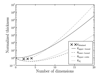
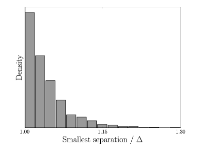
To try to obtain an upper bound on the thickness of the stochastic template bank one can consider the sphere-packing problem, this is the question of how many non-overlapping spheres can be packed into a certain volume. Consider the packing problem with hard spheres of radius . Since the centers of any of these spheres are distances of or more apart, they are suitable locations for a stochastic template bank. In Ref. Conway and Sloane (1993) a bound is given on the number of hard spheres of radius that can be placed into a volume . This can be considered as an upper bound on the number of templates that the stochastic algorithm can place. Figure 2 also suggests that this bound may be a reasonable estimate of the thickness of a complete stochastic bank, it can be seen that the average minimum distance between any template and the rest of the bank is close to , as it would be in the sphere packing problem.
However, at least for low dimension (), Figure 1 shows that the a complete stochastic template bank requires considerably fewer templates than this sphere packing upper bound.
It is also useful to compare this with the performance of known lattice algorithms. In this work two different lattice algorithms are considered. The first is the hyper-cubical lattice, where the hyper-cubes of the lattice are just small enough to fit entirely inside a single ball of radius . The side length of such a cube is given by
| (6) |
since the longest diagonal of this -cube is then long. Thus
| (7) |
describes the normalized thickness of a template bank in a hyper-cubic arrangement.
The second lattice algorithm considered in this work is the lattice Conway and Sloane (1993); Prix (2007). The 2 dimensional lattice is the well known hexagonal lattice. For this algorithm the normalized thickness is given by Messenger et al. (2009)
| (8) |
From Figure 1 it can be seen that the lattice requires less templates than the hyper-cubic lattice in all dimensions (except the trivial one-dimensional case). It is also the most efficient lattice known in dimensions up to 20 Conway and Sloane (1993). This figure also shows that the number of templates required to create a complete stochastic bank is less than the hyper-cubic lattice, but only when the dimension is greater than 3. A stochastic template bank with full coverage, however, will require more templates than the lattice at least up to four dimensions. We have no reason to believe that a complete stochastic bank will be more efficient than the lattice in any dimension.
One must consider however that these lattice algorithms are only defined in the case of flat parameter spaces. The stochastic algorithm on the other hand can be used in any parameter space and it is in the cases where the parameter space is not flat that we believe the stochastic bank would be the most useful.
II.2 The convergence of a stochastic template bank
In real world applications it may not be necessary for the template bank to be complete. It is therefore useful to be able to understand the convergence of the iteration that creates a stochastic template bank. This sub-section is devoted to trying to understand this convergence and comparing it to the method describe in Messenger et al. (2009).
To begin to understand how a stochastic bank converges it is necessary to define a covering fraction . The covering fraction is the ratio of the volume of the subset of that lies within a distance of the points in the template bank, to the total volume of . The expected number of trials required to add a new template to the list is given by , as can be seen by considering the template placement process as a form of Monte-Carlo integration.
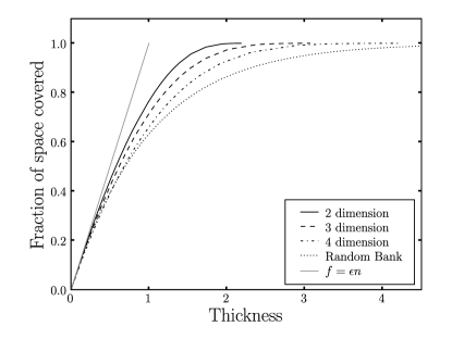
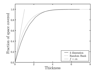
At the beginning of the iterative process, the template bank is empty, and . After the first template is added (and assuming that boundary effects can be ignored!) the covering fraction is , where , which is the fraction of the entire volume covered by a single template. During the first iterative steps, while the number of templates in the bank is small, , the covering fraction increases linearly with the template number according to .
How does the covering fraction increase when becomes larger? To understand this, it is helpful to first consider the behavior that the covering fraction would have in the case where the points in the template bank were simply selected at random from , without any consideration of whether or not they were closer together than . This case is considered in some detail in a recent paper on random template banks Messenger et al. (2009). (In contrast, this paper uses the name stochastic template bank.) In that case, since on average each additional template removes a fraction of the volume that is not already covered, one obtains
| (9) |
or
| (10) |
for the expectation value of the coverage. For small , this gives a linear increase in the covering fraction, which also describes the stochastic template bank.
Compared to the random template bank, on the average, a stochastic template bank gives higher coverage for a given number of templates. This is illustrated in Figure 3, which shows the covering fraction as a function of thickness, where the signal manifold is a unit box in 2, 3 and 4 dimensions. Thus, if it is desirable to minimize the computation cost because a single template bank is going to be used and re-used many times, the stochastic banks could offer a significant improvement compared with the random ones. The graph does seem to indicate, however, that the stochastic bank converges toward the random case as dimension increases. Further investigation is needed to demonstrate what level of improvement the stochastic bank would have over the random bank at high dimension.
II.3 Computational cost of filtering templates
While the stochastic bank will provide a better coverage for the same number of templates, one must incur an extra computational cost to carry out the filtering stage of the stochastic placement algorithm. This sub-section investigates what this computational cost would be as a function of number of templates and covering fraction.
If every random point was accepted as a template, because it was farther than from all previous templates, then the computational cost would be
| (11) |
where is the cost of computing the distance between two points. This follows because the distance must be calculated between all possible pairs of templates, and there are such pairs. This also correctly describes the cost of stochastic template bank creation when the covering fraction is substantially less than one, and few potential templates are rejected. But when the covering fraction approaches one, the computational cost explodes, because the dominant computational cost is the cost of rejecting templates. This is shown in Figure 4.
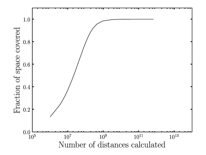
This also allows us to provide an estimate of the computational cost. In practice, 100% coverage is not necessary or desired. For a typical binary inspiral search one might be happy with a coverage . For such coverages the computation cost is bounded above by
| (12) |
which is obtained by assuming that the cost of adding the last template is the same as the cost of adding every template. This is an upper bound because the factor of is larger than , and because the computational cost of adding the earlier templates is smaller than that of adding the final template.
The computational cost of this method grows faster than the square of the number of templates. However, there is a modified version of this algorithm in development that has a cost proportional to . This maintains an internal list of hyper-cubic cells, which contain points separated by distances of less than . When a new random template is considered, its distance only needs to be compared to the points in the same cell, and the neighboring cells. The process of looking to see if there are neighboring cells requires a binary search in an index list, and accounts for the additional factor.
It is this prohibitive computational cost that has prevented us from being able to test the stochastic template bank in dimensions higher than 4 without boundary effects becoming rather pronounced. With this improved version of the algorithm it is hoped that a test of the stochastic bank in higher dimensions can be performed.
III Testing the algorithm
This section investigates how the stochastic template placement performs in dimensions less than 5 and how this compares with geometrical placement algorithms. An investigation of how the algorithm performs when the distribution of initial seed points is not proportional to the determinant of the metric is carried out as well as a demonstration that the stochastic algorithm will perform well in intrinsically curved parameter spaces.
III.1 Templates in flat spaces of different dimensions
First consider a flat unit hyper-cube in -dimensions, with Cartesian coordinates and the metric Each coordinate lies in the range . is chosen so that is equal to 10000.
Figures 3 and 4 show the coverage, in 2, 3 and 4 dimension, and computational cost as a function of the number of templates in the bank. The coverage in Fig. 3 was computed using Monte-Carlo integration with 20,000 sample points. The coverage is the fraction of these points that are less than from a template in the bank. To generate Fig. 3 as well as Figures 5, 4, 9 and Tables 1 and 2 this process was carried out 100 times and the mean of the values obtained was used.
Figure 1 compares the number of templates being converged upon by the stochastic bank with the estimates and the lattice algorithms as described in section II. It can be seen from this table that the stochastic template banks perform better than the naive hyper-cubic lattices as the dimension of the parameter space increases. This is what was predicted in the previous section: the stochastic template banks converge to “complete” coverage with fewer templates than would be needed in a cubic lattice. Also, as predicted, the lattice is more efficient than the stochastic bank when the stochastic bank has reached complete coverage.
An interesting feature, which is more noticeable when the number of templates in the banks is reduced, is that they show effects due to the boundaries, especially noticeable in the higher dimensions. This is easy to understand. Any template located closer than distance to the boundary of the unit cube will have part of its coverage region lying outside the cube. Consequently, if is too large, then many of the templates will fail to produce the amount of coverage that would arise if no boundaries were present. Thus, a sign that boundary effects are appearing is that the initial coverage grows more slowly with template number than expected.
This effect can be seen in Figure 5 where the initial slope at is smaller than unity and also the final thickness is much larger than the estimate, which was not seen in Figure 3. At what template radius do boundary effects become significant? This can be easily understood by estimating the volume that lies within distance of the boundary of the cube. This is . Hence the initial coverage, when is
| (13) |
Here is a numerical factor, of order in three dimensions, which measures the average fraction of volume of a template that lies outside the cube, as the center of the template moves through all positions in the .
III.2 Choice of coordinate system and convergence of template numbers
How does the convergence of the stochastic template bank generation depend upon the distribution of the random template candidates in the underlying parameter space? This question is of practical interest, because the optimal distribution of the random points has a probability proportional to the the volume element . However, it can be difficult in practice to generate such a distribution, whereas it is simple to generate random points that have a uniform distribution in the coordinates.
| Cartesian | Polar | |||||||
|---|---|---|---|---|---|---|---|---|
| 1500 | 1397.1 | 1.0 | 0.1353 | 0.0003 | 1313.4 | 1.3 | 0.1246 | 0.0003 |
| 5000 | 3994.4 | 2.6 | 0.3632 | 0.0004 | 3613.9 | 2.6 | 0.3237 | 0.0004 |
| 15000 | 8494.5 | 3.9 | 0.6818 | 0.0004 | 7605.3 | 3.9 | 0.6140 | 0.0004 |
| 50000 | 13961.5 | 4.1 | 0.9221 | 0.0002 | 12979.6 | 4.0 | 0.8825 | 0.0003 |
| 150000 | 17307.8 | 4.0 | 0.9847 | 0.0001 | 16676.6 | 3.6 | 0.9747 | 0.0001 |
| 500000 | 19365.5 | 3.1 | 0.99746 | 0.00004 | 19025.4 | 3.5 | 0.99582 | 0.00005 |
| 1500000 | 20439.3 | 3.0 | 0.99949 | 0.00001 | 20241.3 | 3.6 | 0.99917 | 0.00002 |
| 5000000 | 21141.9 | 3.5 | 0.99990 | 0.00001 | 21023.4 | 3.2 | 0.99987 | 0.00001 |
| 10000000 | 21401.3 | 3.1 | 0.999971 | 0.000003 | 21305.4 | 3.3 | 0.999948 | 0.000005 |
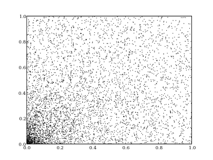
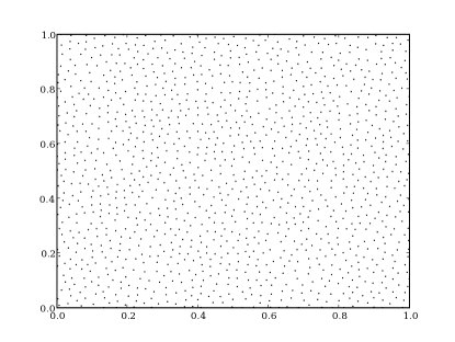
For example, in two-dimensional flat space, one could choose trial points with uniform probability distributions in polar coordinates. This means that too many random templates are tested from the region near the origin, and then rejected. However, they are soon rejected, as being too close to points already in the template bank, and in the end, the template points that survive have the correct probability distribution proportional to . This is shown in Figure 6.
Table 1 shows the number of templates as a function of the number of trial points for random template candidates distributed uniformly in Cartesian and polar coordinates. Also shown is the coverage of the template bank, calculated using Monte-Carlo integration as described in the previous section.
This is very useful because in many cases one does not know coordinates in which the determinant of the metric is constant. Of course one could simply distribute points with a probability density proportional to the volume measure!
III.3 Templates on a sphere
So far the paper has considered templates in a flat signal space. However one can consider examples where the signal manifold is not flat, but is curved. This introduces two new issues.
First, the distance between widely separated points can no longer be easily computed. However, the only important case is the one in which the points are nearby. In this case, one can use the metric to approximate the distance at small separations:
| (14) |
Since the components of the metric can be expensive to calculate, an efficient approach is to calculate and store those components only for points that are included in the template bank. Those metric components are then used for the distance comparisons with potential new (randomly chosen) template candidates.
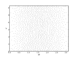
Second, depending upon the choice of the coordinate system, the determinant of the metric may be non-constant. In this case, an efficient approach would be to generate random points with a probability distribution proportional to the volume element . However, in practice one can generate points with any distribution in the coordinates: the stochastic template placement algorithm simply rejects those points that are not needed, and produces a distribution with the correct density proportional to .
To demonstrate the performance of the stochastic template placement algorithm on a curved manifold, consider a unit-radius two-sphere with standard spherical polar coordinates . The metric is
| (15) |
Table 2 shows the number of templates as a function of the number of trial points The size of the templates has been chosen so that the ratio is the same as for the unit cube examples given in the previous section. In this case the stochastic algorithm converges for a smaller number of templates than for the unit cube. This is for the reasons described above: since the unit sphere has no boundary, no templates lie partly outside the space, so every template provides the largest possible coverage.
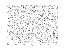
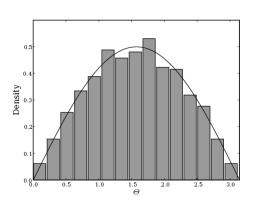
Fig. 7 shows the distribution of 5000 candidate points, chosen uniformly in spherical polar coordinates (top panel). The points that survive and remain in the stochastic template bank are shown in the middle panel. A histogram of the distribution of the templates as a function of is also shown (right panel). As expected, the density of templates is proportional to the volume element : it is smallest at the poles and the greatest at the equator.
IV Templates for gravitational wave chirps
Binary systems of compact objects (i.e., black holes and/or neutron stars) evolve by emitting gravitational radiation. The loss of energy and angular momentum into gravitational waves causes the two bodies to spiral in toward each other, emitting a burst of radiation just before they merge. Although there is no exact solution to the two-body problem in general relativity, an approximation method called the post-Newtonian formalism has been used to compute the amplitude and phase of the waves emitted in the adiabatic inspiral phase to a very high accuracy Blanchet et al. (2002, 2004); Arun et al. (2004) (for a recent review see Ref. Blanchet (2002)). Moreover, recent progress in numerical relativity has provided a good knowledge of the waveform even in the strong gravity regime of the merger dynamics Pretorius (2005). Thus, one can use matched filtering to dig out astrophysical signals from the noise background of an interferometric detector.
In general, the radiation from a binary is characterized by as many as seventeen parameters. However, some of these parameters (the distance to the binary, the inclination of the orbit relative to the detector, etc.) only affect the amplitude of the waveform, which does not modify the search template. Therefore, one would only need to place templates in a lower-dimensional parameter space (say six or seven dimensions). State-of-the-art template placement algorithms deal only with a binary composed of non-spinning objects (in which case templates are only needed in the two-dimensional parameter space of the masses of the component stars) or at best a simplified model of a binary composed of spinning objects requiring one, or two, additional dimensions. Clearly, this is not satisfactory as there is no reason to believe that an astronomical binary will respect simplified models.
The goal of the stochastic template placement algorithm is to address the problem of choosing templates on a manifold of arbitrary dimensions. However, in this paper, the algorithm is only applied to the case of a binary consisting of non-spinning bodies where the results are well known, thus facilitating a straightforward comparison with established results. This algorithm has also been applied in a recent search for spinning binaries in the first year of LIGO’s fifth science run using templates placed in a three-dimensional parameter space Van Den Broeck et al. (2009) as well as a five-dimensional search for super-massive black holes in a mock data challenge Harry et al. (2009). A similar, but independently developed, algorithm was also used in this mock data challenge Babak (2008). This algorithm was effectively the same as the one described in this work but the author calculates the overlap between points explicitly, instead of using the metric approximation as in this work. While this will more accurately determine the overlap, especially for overlaps not close to unity, it will come at considerable additional computational cost.
| 1500.0 | 1330.3 | 1.2 | 0.1989 | 0.0004 |
|---|---|---|---|---|
| 5000.0 | 3688.3 | 2.8 | 0.4253 | 0.0004 |
| 15000.0 | 7807.1 | 3.7 | 0.7027 | 0.0004 |
| 50000.0 | 13198.7 | 4.1 | 0.9192 | 0.0002 |
| 150000.0 | 16779.5 | 4.4 | 0.9836 | 0.0001 |
| 500000.0 | 19007.0 | 3.6 | 0.99735 | 0.00003 |
| 1500000.0 | 20171.6 | 3.6 | 0.99947 | 0.00002 |
| 5000000.0 | 20906.6 | 3.8 | 0.99991 | 0.00001 |
| 10000000.0 | 21182.9 | 4.0 | 0.999967 | 0.000004 |
IV.1 Choice of coordinate system
Begin by choosing a suitable coordinate system on the signal manifold. The masses and of the component stars are the most obvious coordinates on the manifold. However, when one uses masses as the coordinate system the determinant of the metric will vary significantly over this parameter space Owen and Sathyaprakash (1999). Because of this a much higher density of templates is needed in the low mass region than in the high mass region.
A better coordinate system is chirp times Sathyaprakash (1994), defined by
| (16) |
| (17) |
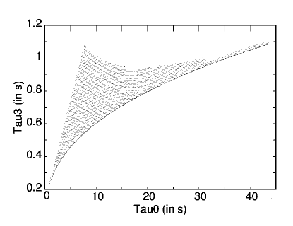
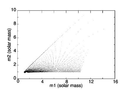
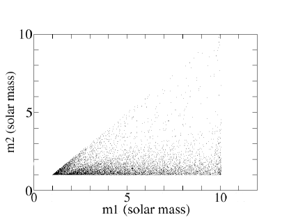
Using this coordinate system the determinant of the metric does not vary much over this parameter space. This can be illustrated by looking at the distribution of templates in both coordinate-systems as shown in Figure 8. The algorithm used in this case Cokelaer (2007) places templates first along the curve (the lower right boundary in the left panel and upper left boundary in the right panel). This is dictated by the fact that the region below the equal-masses curve (in , coordinates) corresponds to binaries with imaginary component masses111Although the waveform, which depends only on the total mass and mass ratio which are real in that region, can be generated in this part of the parameter space, it is unphysical and, therefore, not of any interest.. The algorithm uses a hexagonal placement over the rest of the parameter space.
IV.2 Comparison of stochastic lattice with a square lattice
Let us now compare the stochastically generated template bank with a hexagonal lattice and with a square lattice. In this case the template banks are created to cover binary compact objects whose components have a mass range of 1 to 10 solar masses such that any real signal within this range of masses would have an “overlap” greater than 0.96 with at least one of the templates in the bank. This overlap, defined by , is calculated using the assumption made in equation (14) and the metric defined in Babak et al. (2006). For the stochastic algorithm the trial points are placed uniformly in coordinates (and limited by the restrictions on the masses). This is also compared to trial points placed uniformly in coordinates.
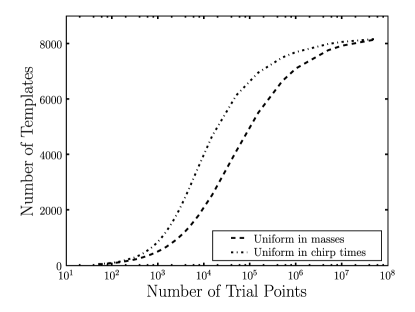
For this choice of parameters and for trial points placed uniformly in both coordinate systems, the number of templates is plotted as a function of the number of trial points in Fig. 9. Fig. 10 shows the distribution of resultant templates for both initial trial point distributions.
In this two-dimensional example, the stochastic algorithm, in both cases, converges at about 7500 templates. For comparison, with the same range of masses a hexagonal lattice has 5914 templates and and a square lattice has 8353 templates. This may seem to be in conflict with the statement in section II that the stochastic algorithm performs worse than hyper-cubic lattices in two dimensions. However, one must remember that the geometrical algorithm used here begins by placing templates along the boundaries, which is quite inefficient. One also must remember that though this parameter space is close to flat it is not flat.

IV.3 Efficiency of the Stochastic bank
The quality or performance of a template bank can be assessed by measuring the overlap between randomly simulated compact binary signals in the relevant range of parameters of the template bank in question. To test the performance of the stochastic template banks, a set of 20,000 signals (standard post-Newtonian waveforms of type TaylorT3 Damour et al. (2001)) was generated and the maximum overlap of each over the entire template bank was calculated. In this case templates with masses between 3 and 30 solar masses were used (a different mass range was used here to produce less templates, thus making it easier to show the results graphically) and an overlap of 0.95 was used, equivalently, . The template bank was generated from 60,000 trial points placed uniformly in coordinates.
The result of the test is shown in Fig. 11. One can see that the stochastic placement algorithm struggles to cover certain areas of this parameter space. If a larger number of trial points had been used, the coverage would have been better.
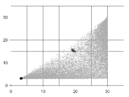
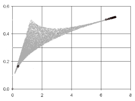
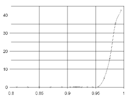
The areas of the parameter space with poor coverage from the stochastic template bank are in regions of the parameter space that are very thin, almost one-dimensional. The hexagonal and square lattices also have this difficulty but they have been specifically designed to overcome this problem by placing templates along the boundary of the space, especially along the curve. A stochastic placement algorithm can overcome this problem in the same manner, or by increasing the mass range of allowed templates. But both solutions come with the cost of additional templates in the bank.
V Conclusions
This paper presents a method for stochastically generating template banks in parameter spaces of arbitrary dimension and with arbitrary metrics. The relationship between coverage and the number of templates required to reach that coverage has been investigated for dimensions up to 4. The performance of the stochastic placement algorithm has been compared to lattice placement algorithms in flat spaces and was found to only be marginally less effective at dimension less than 4. The area where we believe this algorithm would be of most use is in signal manifolds that have a large intrinsic curvature, where lattice placement algorithms can not easily be applied. Stochastic banks which cover less than 100% of the signal manifold may be useful for large dimensional manifolds, though further investigation is needed to show that this is the case.
For cases where the number of required templates is very high, the algorithm will become very computationally expensive. In these cases other “random template banks”, which do not use our filtering stage might become more practical Messenger et al. (2009). Nevertheless the stochastic template bank will provide better coverage for a given number of templates. The construction of stochastic template banks can be made less expensive, however, by utilizing the fact that it is not necessary to compute the distance between a trial point and every template in the bank. This is a topic of ongoing investigation.
Acknowledgements
We would like to thank Reinhard Prix, Thomas Dent, Stephen Fairhurst, Gareth Jones and Gian Mario Manca for their useful comments and feedback in bringing this paper to fruition. In this work IWH was supported by the Science and Technology Facilities Council, UK, studentship ST/F005954/1, BA was partly supported by US National Science Foundation grant PHY-0701817 and BSS was supported by Science and Technology Facilities Council, UK, grant PP/F001096/1. This paper has been assigned LIGO document number P0900069-v3.
References
- Acernese et al. (2006) F. Acernese et al., Class. Quant. Grav. 23, S635 (2006).
- Abbott et al. (2009a) B. Abbott et al., Reports on Progress in Physics 72, 076901 (25pp) (2009a).
- Abbott et al. (2007a) B. Abbott et al. (LIGO Scientific Collaboration), Phys. Rev. D76, 042001 (2007a), eprint gr-qc/0702039.
- Abbott et al. (2007b) B. Abbott et al. (LIGO Scientific Collaboration), Class. Quant. Grav. 24, 5343 (2007b), eprint arXiv:0704.0943 [gr-qc].
- Abbott et al. (2009b) B. Abbott et al. (LIGO Scientific Collaboration), Phys. Rev. D79, 122001 (2009b).
- Thorne (1987) K. S. Thorne, in Three hundred years of gravitation, edited by S. Hawking and W. Israel (Cambridge University Press, 1987), pp. 330–458.
- Helström (1968) C. Helström, Statistical Theory of Signal Detection, vol. 9 of International Series of Monographs in Electronics and Instrumentation (Pergamon Press, Oxford, U.K., New York, U.S.A., 1968), 2nd ed.
- Schutz (1989) B. Schutz, in The detection of gravitational waves, edited by D. Blair (Cambridge University Press, England, 1989), pp. 406–452.
- Sathyaprakash and Dhurandhar (1991) B. S. Sathyaprakash and S. V. Dhurandhar, Phys. Rev. D44, 3819 (1991).
- Dhurandhar and Sathyaprakash (1994) S. V. Dhurandhar and B. S. Sathyaprakash, Phys. Rev. D49, 1707 (1994).
- Sathyaprakash (1994) B. S. Sathyaprakash, Phys. Rev. D50, 7111 (1994), eprint gr-qc/9411043.
- Balasubramanian et al. (1995) R. Balasubramanian, B. S. Sathyaprakash, and S. V. Dhurandhar, Pramana 45, L463 (1995), eprint gr-qc/9508025.
- Balasubramanian et al. (1996) R. Balasubramanian, B. S. Sathyaprakash, and S. V. Dhurandhar, Phys. Rev. D 53, 3033 (1996), erratum-ibid. D 54, 1860 (1996), eprint gr-qc/9508011.
- Owen (1996) B. Owen, Phys. Rev. D 53, 6749 (1996).
- Owen and Sathyaprakash (1999) B. Owen and B. S. Sathyaprakash, Phys. Rev. D 60, 022002 (1999).
- Brady et al. (1998) P. R. Brady, T. Creighton, C. Cutler, and B. F. Schutz, Phys. Rev. D 57, 2101 (1998), eprint gr-qc/9702050.
- Babak et al. (2006) S. Babak, R. Balasubramanian, D. Churches, T. Cokelaer, and B. Sathyaprakash, Class. Quant. Grav. 23, 5477 (2006), eprint gr-qc/0604037.
- Cokelaer (2007) T. Cokelaer, Phys. Rev. D76, 102004 (2007), eprint arXiv:0706.4437 [gr-qc].
- Prix (2007) R. Prix, Classical and Quantum Gravity 24, S481 (2007).
- Messenger et al. (2009) C. Messenger, R. Prix, and M. A. Papa, Phys. Rev. D79, 104017 (2009).
- Conway and Sloane (1993) J. Conway and N. Sloane, Sphere Packings, Lattices and Groups (Springer-Verlag, New York, 1993), 2nd ed.
- Blanchet et al. (2002) L. Blanchet, G. Faye, B. R. Iyer, and B. Joguet, Phys. Rev. D 65, 061501(R) (2002), Erratum-ibid 71, 129902(E) (2005), eprint gr-qc/0105099.
- Blanchet et al. (2004) L. Blanchet, T. Damour, G. Esposito-Farèse, and B. R. Iyer, Phys. Rev. Lett. 93, 091101 (2004), eprint gr-qc/0406012.
- Arun et al. (2004) K. G. Arun, L. Blanchet, B. R. Iyer, and M. S. S. Qusailah, Class. Quantum Grav. 21, 3771 (2004), erratum-ibid. 22, 3115 (2005), eprint gr-qc/0404185.
- Blanchet (2002) L. Blanchet, Living Rev. Rel. 5, 3 (2002), eprint gr-qc/0202016.
- Pretorius (2005) F. Pretorius, Phys. Rev. Lett. 95, 121101 (2005), eprint gr-qc/0507014.
- Van Den Broeck et al. (2009) C. Van Den Broeck et al. (2009), eprint arXiv:0904.1715 [gr-qc].
- Harry et al. (2009) I. Harry, S. Fairhurst, and B. Sathyaprakash, Class. Quantum Grav. 25, 184027 (2009).
- Babak (2008) S. Babak, Class. Quant. Grav. 25, 195011 (2008), eprint 0801.4070.
- Damour et al. (2001) T. Damour, B. R. Iyer, and B. S. Sathyaprakash, Phys. Rev. D 63, 044023 (2001), erratum-ibid. D 72 (2005) 029902, eprint gr-qc/0010009.