Interpolating compact binary waveforms using the singular value decomposition

Abstract

Compact binary systems with total masses between tens and hundreds of solar masses will produce gravitational waves during their merger phase that are detectable by second-generation ground-based gravitational-wave detectors. In order to model the gravitational waveform of the merger epoch of compact binary coalescence, the full Einstein equations must be solved numerically for the entire mass and spin parameter space. However, this is computationally expensive. Several models have been proposed to interpolate the results of numerical relativity simulations. In this paper we propose a numerical interpolation scheme that stems from the singular value decomposition. This algorithm shows promise in allowing one to construct arbitrary waveforms within a certain parameter space given a sufficient density of numerical simulations covering the same parameter space. We also investigate how similar approaches could be used to interpolate waveforms in the context of parameter estimation.

I Introduction

Searches for gravitational waves from binary black holes with total masses between tens and hundreds of solar masses benefit from the complete model of the gravitational waveform obtained by numerical relativity Flanagan and Hughes (1998); Hanna (2010). Numerically solving Einstein’s equations is now quite routine Pretorius (2005); Campanelli et al. (2006); Baker et al. (2006); Pretorius (2009); Husa (2007); Hannam (2009); Hinder (2010), yet still computationally burdensome. Reference Baumgarte et al. (2008) suggests that there is a finite density of numerical simulations that would adequately cover the parameter space for certain ground-based detectors. In this work we explore this concept and extend the numerical techniques presented in Cannon et al. (2010) and Cannon et al. (2011), to interpolation of template waveforms using the singular value decomposition. This should allow for the construction of gravitational waveforms with parameters between the numerically generated waveforms.

The idea of interpolating gravitational waveforms has existed for over a decade. Interpolation of waveforms generated by post-Newtonian techniques was described in Croce et al. (2000) and Mitra et al. (2005). In these references analytic formulae for waveform interpolation were derived for particular PN models. Since 2005 the numerical relativity community has been generating a substantial number of gravitational waveforms for the coalescence of binary black holes Pretorius (2005); Campanelli et al. (2006); Baker et al. (2006); Pretorius (2009); Husa (2007); Hannam (2009); Hinder (2010). Interpolation of these waveforms has been accomplished primarily by (i) phenomenologically fitting the simulations to closed-form expressions Ajith et al. (2007, 2008, 2009) or (ii) by numerically solving simpler differential equations that capture the orbital dynamics combined with numerical stitching of the ringdown phase Buonanno et al. (2007a); Damour et al. (2008); Buonanno et al. (2007b); Damour et al. (2008, 2008); Damour and Nagar (2009); Buonanno et al. (2009). In this work we propose a different approach to interpolate a set of template waveforms. This approach does not require careful tuning of fitting formulae or stitching of waveforms and can be applied to any waveform set of sufficient density.

This paper is organized as follows. First, we describe the technique for interpolating waveforms via the singular value decomposition. Second we apply the technique to a set of waveforms containing all phases of the compact binary coalescence, inspiral, merger and ringdown. Third we discuss how these results might be applied to the contruction of waveform families, ongoing gravitational wave searches, and parameter estimation.

II Interpolation technique

It was shown in Cannon et al. (2010) that the singular value decomposition (SVD) reduces the number of template waveforms needed to search a given parameter space. Additionally, Cannon et al. (2011) showed that arbitrary waveforms within the parameter space could be reconstructed from the SVD of a sufficiently dense template bank. Here we demonstrate a method to directly obtain approximate reconstruction coefficients for arbitrary waveforms in the parameter space via interpolation. Consider a waveform family ${\bf h}(x,y)$ described by the physical parameters $(x,y)$, and consider a set of these waveforms enumerated by the index $\alpha$ drawn from a region of the parameter space, ${\bf h}(x_{\alpha},y_{\alpha})$. Recall that a SVD of these waveforms allows each to be written as a linear combination of basis waveforms ${\bf u}_{\mu}$ with coefficients $M_{\mu}(x_{\alpha},y_{\alpha})$

$${\bf h}(x_{\alpha},y_{\alpha})=\sum_{\mu}M_{\mu}(x_{\alpha},y_{\alpha})\,{\bf u}_{\mu},$$ (1)

where, in the formalism of Cannon et al. (2010) and Cannon et al. (2011), $M_{\mu}(x_{\alpha},y_{\alpha}):=\sigma_{\mu}(v_{(2\alpha-1)\mu}+\mathrm{i}v_{(2\alpha)\mu})$ is the $\alpha$th combination of singular values $\sigma_{\mu}$ and reconstruction coefficients $v_{(2\alpha-1)\mu}$ and $v_{(2\alpha)\mu}$. Recall also that waveforms with arbitrary physical parameters from the same region of parameter space can also be reconstructed using the basis vectors ${\bf u}_{\mu}$ by projecting the waveforms onto the basis vectors to obtain the reconstruction coefficients—a computationally expensive procedure,

$${\bf h}(x,y)\approx\sum_{\mu}({\bf h}(x,y)\cdot{\bf u}_{\mu})\,{\bf u}_{\mu}.$$ (2)

This can be used to define the arbitrary reconstruction coefficients as

$$M_{\mu}(x,y)={\bf h}(x,y)\cdot{\bf u}_{\mu}.$$ (3)

We seek the set of interpolated reconstruction coefficients $M_{\mu}^{\prime}(x,y)$ that can approximately reconstruct an arbitrary waveform from that region of parameter space.

Compact binary gravitational waveforms with negligible effects from spin and eccentricity are characterized by their component masses. We will assume for concreteness a two parameter family of waveforms ${\bf h}(x,y)$ where $x$ and $y$ are $M$ and $q$, respectively, where $M=m_{1}+m_{2}$ is the total mass of the system and $q=m_{1}/m_{2}$ is the mass ratio of the system.

Chebyshev polynomials of the first kind are known to be good for interpolation, however other interpolation schemes are also possible. We start with a set of basis vectors ${\bf u}_{j}$ covering the desired region of parameter space. We choose a net of points, scaled such that each dimension covers the interval $[-1,1]$, located at the ${J_{\mathrm{max}}}$th order Chebyshev nodes. For a single dimension, these nodes occur at the locations

$$x_{j}=\cos\left(\pi\frac{j+\frac{1}{2}}{{J_{\mathrm{max}}}+1}\right),$$ (4)

where $j$ ranges from 0 to ${J_{\mathrm{max}}}$. This choice of net reduces Runge’s phenomenon when used with the Chebyshev polynomials, which, for a single dimension, are given as

$$T_{J}(x)=\frac{(x-\sqrt{x^{2}-1})^{J}+(x+\sqrt{x^{2}-1})^{J}}{2w},$$ (5)

where $w=\sqrt{(1+\delta_{J0})({J_{\mathrm{max}}}+1)/2}$ is a normalization factor for the polynomials and $\delta_{J0}$ is the Kroenecker delta. Both $x_{j}$ and $w$ depend on the choice of ${J_{\mathrm{max}}}$, however for ease of notation we will leave this implied. The polynomials $T_{J}(x)$ satisfy the discrete orthogonality condition

$$\sum_{j=0}^{{J_{\mathrm{max}}}}T_{I}(x_{j})T_{J}(x_{j})=\delta_{IJ}.$$ (6)

It is straightforward to extend this to higher dimensions.

In order to obtain the reconstruction coefficients for these locations, we project waveforms from these locations onto the basis vectors. From the values on this net, we interpolate to other positions in parameter space using 2D-Chebyshev interpolation for each set of reconstruction coefficients $M_{\mu}(x,y)$. Specifically, these values are projected onto the Chebyshev polynomials

$$C_{KL\mu}=\sum_{k=0}^{{K_{\mathrm{max}}}}\sum_{l=0}^{{L_{\mathrm{max}}}}T_{K}(x_{k})T_{L}(y_{l})M_{\mu}(x_{k},y_{l}).$$ (7)

This results in coefficients for the 2D-Chebyshev polynomials which can be used to evaluate the interpolated reconstruction coefficients $M_{\mu}^{\prime}(x,y)$ at other points in parameter space

$$M_{\mu}^{\prime}(x,y)=\sum_{K=0}^{{K_{\mathrm{max}}}}\sum_{L=0}^{{L_{\mathrm{max}}}}C_{KL\mu}T_{K}(x)T_{L}(y).$$ (8)

In the next section we explore this approximation technique using gravitational waveforms containing all three phases of binary coalescence, inspiral, merger and ringdown.

II.1 Reconstruction Errors

Errors in reconstructing these waveforms come in two types: errors due to SVD truncation, and errors due to reconstruction coefficient interpolation. The truncation errors have previously been shown to take the form

$$\left(\frac{\delta\rho(x,y)}{\rho(x,y)}\right)_{\rm trunc}=\frac{1}{4}\sum_{\mu=N^{\prime}+1}^{N}|M_{\mu}(x,y)|^{2},$$ (9)

where the sum is over the basis vectors that are discarded. The interpolation errors have a similar form

$$\left(\frac{\delta\rho(x,y)}{\rho(x,y)}\right)_{\rm interp}=\frac{1}{4}\sum_{\mu=1}^{N^{\prime}}|M_{\mu}(x,y)-M_{\mu}^{\prime}(x,y)|^{2}.$$ (10)

It should be noted that here the sum is over the basis vectors that are kept from the SVD. By setting the reconstruction coefficients with $\mu>N^{\prime}$ to zero, these can be combined into a single expression

$$\frac{\delta\rho(x,y)}{\rho(x,y)}=\frac{1}{4}\sum_{\mu=1}^{N}|M_{\mu}(x,y)-M_{\mu}^{\prime}(x,y)|^{2}.$$ (11)

III Results

We apply this procedure in two ways. In section III.1 we investigate using this approach in the context of interpolating whitened waveforms. This would be useful in the context of parameter estimation. Specifically, one could obtain reconstruction coefficients that would be used for constructing filter outputs associated with arbitrary points in parameter space using the filter outputs from the SVD basis vectors.

In section III.2, we apply similar techniques to interpolate raw waveforms. This is done in the context of waveforms one would receive from numerical relativity simulations (i.e., time series of $\Psi_{2}(t)=\partial_{t}^{2}h_{+}(t)+\mathrm{i}\partial_{t}^{2}h_{\times}(t)$ that are restricted to lie along lines of constant $M$). This approach could be taken to extend numerical relativity waveform catalogs at greatly reduced computational cost.

III.1 Whitened waveforms

We apply this procedure to non-spinning phenomenological inspiral-merger-ringdown (IMR) waveforms Ajith et al. (2009) with $M\in[60M_{\odot},80M_{\odot}]$, $q\in[1,10]$, whitened with an initial LIGO amplitude spectral density (ASD), and transformed to the time domain. We generate a stochastic template bank Harry et al. (2009) with $99\%$ minimal match for this range of parameters. Since we are working with IMR waveforms, there is no well defined end of the waveform. We choose to align the whitened waveforms according to their peak amplitudes and compute the SVD basis vectors from these waveforms using the procedure described in Cannon et al. (2010). At this intermediate stage, if we were to look at how the resulting reconstruction coefficients vary in parameter space, we would see high frequency features that would be difficult to resolve with interpolation without a high density interpolation net.

Figure 1: Reconstruction coefficients as a function of $M$ and $q$ associated with the $3^{\rm rd}$ and $21^{\rm st}$ basis vectors are shown in the left and right columns, respectively. The top row shows the real part of the reconstruction coefficients. The bottom row shows the imaginary part of the reconstruction coefficients.

Fortunately, these features can be ameliorated by a complex rotation of the input waveforms, which is equivalent to a complex rotation of the reconstruction coefficients,

$$M_{\mu}(x,y)\rightarrow e^{-\mathrm{i}\arg M_{1}(x,y)}M_{\mu}(x,y).$$ (12)

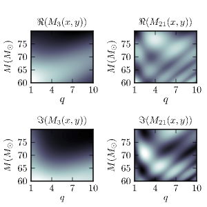
This rotation is chosen such that $\Im\left[M_{1}(x,y)\right]=0$. Fig. 1 shows the reconstruction coefficients associated with the $3^{\rm rd}$ and $21^{\rm st}$ basis vectors after this complex rotation. The smoothness of these reconstruction coefficients indicates that interpolation should be possible.

Figure 2: The upper panel shows the fitting factor residual associated with using the interpolation net as templates in a template bank. The lower panel shows the interpolation mismatch for waveforms from with the parameter space. The interpolation mismatch is more than an order of magnitude smaller than the fitting factor residual.

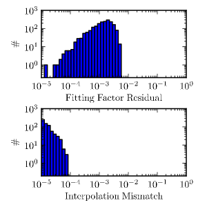
In order to perform the interpolation, waveforms from the (12,12) order 2D-Chebyshev net are then projected onto these basis vectors to obtain the interpolation coefficients, as described by (7), and rotated as described above. $40\times 40$ test waveforms from within the parameter space, laid out in a grid, are used for computing mismatches between the interpolated waveforms, given by (8), and the original waveforms. Fig. 2 compares the fitting factor residual, which we define to be one minus the fitting factor, obtained from using the net waveforms as templates with the interpolation mismatches associated with the test waveforms. We see that the largest interpolation mismatch is more than an order of magnitude smaller than the fitting factor residual from the net waveforms.

III.2 Raw waveforms

We apply similar techniques to waveforms of a type that would be provided by numerical relativity simulations. Specifically, we use non-spinning phenomenological IMR waveforms Ajith et al. (2009) with $M\in[60M_{\odot},80M_{\odot}]$, $q\in[1,6]$, multiplied by $f^{2}$, which is equivalent to taking two time-derivatives, and transformed to the time domain. We use the same alignment and rotation techniques described in section III.1 to prepare the waveforms for interpolation.

To generate the basis vectors that enclose this parameter space, we construct a stochastic template bank with an additional constraint. The mass ratios of the templates are restricted to take on values $q\in\{q_{j}=5x_{j}+1|j\in[1,6]\}$, where $x_{j}$ are the nodes associated with the 10th order Chebyshev polynomial.

Figure 3: The upper panel shows the locations for which waveforms were produced, chosen by a stochastic template placement algorithm. These waveforms were used in constructing the basis vectors enclosing this region of parameter space. The lower panel shows the interpolation mismatch for waveforms from within the parameter space. Waveforms interpolation accuracies are below a few times $10^{-4}$.

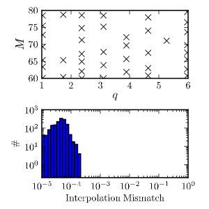
With the basis vectors in hand, we project the waveforms from an interpolation net consisting of the (20,10) 2D-Chebyshev nodes onto the basis vectors to obtain the reconstruction coefficients. These complex coefficients are rotated as described above, and then used to obtain the interpolation coefficients. Again, $40\times 40$ test waveforms from within the parameter space, laid out in a grid, are used for computing mismatches between the interpolated waveforms and the original waveforms. We find comparable interpolation mismatches for these non-whitened waveforms, shown in figure 3, as for the whitened waveforms.

IV Conclusion

Using the procedure described above, we have shown it is possible to produce gravitational waveforms for arbitrary points in parameter space by interpolating reconstruction coefficients from the SVD of a set of waveforms uniformly covering the space.

Results have been presented for both whitened waveforms, and raw waveforms. The former could be useful in the context of parameter estimation associated with compact binary coalescence (CBC) gravitational-wave (GW) signals, which frequently uses Monte Carlo Markov Chain methods to measure the likelihood ratio from many points in parameter space. This requires the generation of the waveforms for each point in parameter space and the overlap computation between the waveform and the data. Using the interpolated reconstruction coefficients, the same computation could be approximately performed with generating a subset of the total waveforms, reconstructing the overlap by appropriately recombining the filter outputs from the basis vectors. The latter could be used to accurately interpolate waveforms that are computationally costly to produce, as is the case for numerical relativity waveforms.

For future work, these techniques should be expanded to include additional dimensions of parameter space (e.g., binary object spin parameters). In addition, other interpolation schemes that use equispaced or random points in parameter space might be found to be favorable for different applications. We also note that these techniques could be applied to other gravitational waveforms such as supernova waveforms where singular value decomposition has also been applied Heng (2009), or where other methods have been used to reduce the rank of the parameter space Field et al. (2011).