Matching post-Newtonian and numerical relativity waveforms: systematic errors and a new phenomenological model for non-precessing black hole binaries
Abstract
We present a new phenomenological gravitational waveform model for the inspiral and coalescence of non-precessing spinning black hole binaries. Our approach is based on a frequency domain matching of post-Newtonian inspiral waveforms with numerical relativity based binary black hole coalescence waveforms. We quantify the various possible sources of systematic errors that arise in matching post-Newtonian and numerical relativity waveforms, and we use a matching criteria based on minimizing these errors; we find that the dominant source of errors are those in the post-Newtonian waveforms near the merger. An analytical formula for the dominant mode of the gravitational radiation of non-precessing black hole binaries is presented that captures the phenomenology of the hybrid waveforms. Its implementation in the current searches for gravitational waves should allow cross-checks of other inspiral-merger-ringdown waveform families and improve the reach of gravitational wave searches.
pacs:
04.80.Nn, 04.30.Db, 04.25.Nx, 04.25.dcI Introduction
As a generalization of the classic Kepler problem in Newtonian gravity, the binary black hole (BBH) system in general relativity is of great interest from a fundamental physics viewpoint. Equally importantly, this system has received a great deal of attention for its relevance in astrophysics and, in particular, as one of the most promising sources of detectable gravitational radiation for the present and future generations of gravitational-wave detectors, such as LIGO Abbott et al. (2009), Virgo Acernese et al. (2008), GEO600 Grote (2008), LISA Shaddock (2009) or the Einstein Telescope Punturo et al. (2010). The Kepler problem can be solved exactly in Newtonian gravity and it leads to the well-known elliptical orbits when the system is gravitationally bound. In contrast, in general relativity, closed orbits do not exist and the BBH system emits gravitational waves (GWs) which carry away energy, thereby causing the black holes to inspiral inwards, and to eventually coalesce. The emitted GWs are expected to carry important information about this process, and it is one of the goals of gravitational wave astronomy to detect these signals and decode them.
No analytic solutions of Einstein’s equations of general relativity are known for the full inspiral and merger of two black holes. Post-Newtonian (PN) methods can be used to calculate an accurate approximation to the early inspiral phase, using an expansion in powers of (where is the orbital velocity and is the speed of light). As for the coalescence phase, starting with Pretorius (2005); Campanelli et al. (2006); Baker et al. (2006), the late inspiral and merger has been calculated by large-scale numerical solutions of the full Einstein field equations. Since the initial breakthroughs in 2005, there has been dramatic progress in numerical relativity (NR) simulations for GW astronomy, including many more orbits before merger, greater accuracy and a growing sampling of the black hole-binary parameter space. A summary of the published “long” waveforms is given in the review Hannam (2009), and a complete catalog of waveforms is being compiled at nin ; more recent work is summarized in Hinder (2010). NR results are now accurate enough for GW astronomy applications over the next few years Hannam et al. (2009), and have started playing a role in GW searches Aylott et al. (2009, 2009).
Given PN and NR results, it is promising to try and combine them to produce “complete” inspiral-merger-ringdown waveforms. PN techniques in their standard formulation become less accurate as the binary shrinks, and the approximation breaks down completely somewhere prior to the merger. NR waveforms, on the other hand, become more and more computationally expensive the larger the number of cycles that one wishes to simulate; the longest published data spans 16 orbits for the equal-mass non-spinning case Scheel et al. (2009). We therefore would hope to combine PN and NR results in the region between the point where NR simulations start and where PN breaks down. To do this it is critical to verify that the PN and NR results are in good agreement in this region and that there is a consistent PN-NR matching procedure. Much work has been done in comparing PN and NR results over the last 5-15 orbits before merger for a variety of physical configurations, such as the equal-mass non-spinning case Buonanno et al. (2007); Baker et al. (2007); Hannam et al. (2008); Gopakumar et al. (2008); Boyle et al. (2007, 2008); Hinder et al. (2008), the equal-mass non-precessing-spin case Hannam et al. (2008), and the unequal-mass spinning case Campanelli et al. (2009). The consistency of PN amplitudes during the merger and ringdown has also been studied Buonanno et al. (2007); Berti et al. (2007, 2008). These studies suggest that a sufficiently accurate combination of PN and NR results should be possible. One topic that has not received much attention, however, is the systematic errors that are introduced by different choices of matching procedure.
One of the aims of this paper is to further understand and quantify the various systematic errors that arise in the matching procedure. There are thus far two kinds of approaches to the PN-NR matching problem, both of which have yielded successful results. The first is the Effective-One-Body (EOB) approach Buonanno and Damour (1999, 2000); Damour et al. (1998, 2000). Originally motivated by similar techniques in quantum field theory, the idea is to map the two body problem into an effective one-body system with an appropriate potential and with the same energy levels as the two-body system. It was shown Buonanno and Damour (1999) that the appropriate one-body problem (for non-spinning black holes) is that of a single particle moving in a deformed Schwarzschild spacetime. It turns out that most parameters of this one-body system can be found by using the appropriate PN calculations, and the remaining parameters are calculated by calibrating to NR simulations. This approach has been successful so far for non-spinning systems where only a few parameters need to be calibrated by NR Buonanno et al. (2007, 2009); Damour et al. (2008, 2008); Damour and Nagar (2009). The spinning case is more complicated, and work is underway to extend the parameter space described by the model Pan et al. (2010).
A complementary approach is to perform a phenomenological matching of the GW waveforms in a window (which could be either in the time or frequency domain) where both PN and NR are expected to be good approximations to the true waveform. The first step is to construct a hybrid PN-NR waveform by matching the two waveforms within the matching window. The waveform is completely PN before this window, completely NR afterward, and it interpolates between the two in the matching window. Once the hybrid waveform is constructed and we are confident about the matching procedure, the second step is to fit the hybrid waveform to a parametrized model containing a number of phenomenological coefficients and finally to map them to the physical parameters of the system. The resulting model would thus be parametrized by the masses and spins of the two black holes (and eccentricity if appropriate). Most of the work in this approach has thus far been based on matching PN and NR waveforms in the time domain, but then producing a phenomenological model in the frequency domain, which is often more convenient for data-analysis applications Ajith et al. (2007); Ajith (2008); Ajith et al. (2008, 2009). See also Sturani et al. (2010) for a complementary construction. In this paper we take a slightly different approach: both the construction of the PN-NR hybrid waveform and the matching to a phenomenological model are carried out in the frequency domain. The reasons for this are twofold. First, we find it easier to work in the frequency domain since the quantities used to estimate the errors of our matching procedure and the goodness of the fit, such as waveform overlaps, are conveniently formulated in Fourier space. Second, and more importantly, in light of the potential errors in the hybrid construction, comparing results between two independent methods is a valuable way of ensuring that the matching procedure is robust. The frequency domain construction presented here is complementary to the time domain method of Ajith et al. (2009).
The phenomenological waveform family presented in Ajith et al. (2009) used a simple piecewise ansatz for the phase of the hybrid PN-NR waveform, and another for the amplitude. The resulting analytic model was found to agree with the hybrid waveforms with overlaps above 97% for most black hole binary systems that would be observable by the current LIGO detectors. In this paper we investigate whether the fidelity of the phenomenological waveforms can be improved by using ansätze that make smooth transitions between their inspiral, merger and rindown forms. This procedure also allows us to further test the robustness of the phenomenological model’s construction to variations in its analytic form.
The main results of this paper are the following. We construct hybrid waveforms for binary black hole systems with aligned spins in the frequency domain. We do this by combining 3.5PN waveforms in the stationary phase approximation with a number of NR results. We show that this construction is internally consistent and it yields hybrids which are, for the most part, sufficiently accurate for the initial and advanced LIGO detectors. Notably, the difference between the different PN approximants is a more significant source of error than the numerical errors in the NR waveforms. Using these hybrid waveforms, we construct a phenomenological frequency-domain waveform model depending on three parameters (as in Ajith et al. (2009)) and covering the space of aligned spins and moderate mass ratios. We show that the model fits the original hybrid waveforms with the overlaps (maximized over the model parameters) better than 97% for Advanced LIGO (and for the most part, better than 99%) for essentially all black hole systems observable with Advanced LIGO, i.e. for systems with total mass ranging up to . These results are comparable to those obtained in Ajith et al. (2009), suggesting that the phenomenological construction is indeed robust and that the phenomenological model waveforms are useful for detection purposes.
Sections II and III describe the post-Newtonian waveform model and the numerical waveforms that we employ. Section IV describes the fitting procedure and the various systematic errors that appear in this procedure. It quantifies the reliability of the waveforms for specific GW detector and signal-to-noise ratios (SNRs). Section V fits these hybrid waveforms to an analytic model. It shows that the model provides a good representation of the hybrid waveforms and can be used in GW searches in the appropriate parameter space. Finally, section VI concludes with a summary and suggestions for future work.
II Numerical simulations of non-precessing black hole binaries
In this section we summarize the numerical waveforms used in this paper. Since the first successful numerical simulations of equal-mass, non-spinning binary black hole mergers were published Pretorius (2005); Campanelli et al. (2006); Baker et al. (2006) the NR community has continued exploring the parameter space of the BBH system. Each black hole is described by a mass and a spin vector, and the binary’s trajectory is described by adiabatically evolving Keplerian orbits, so 17 parameters are needed to describe the binary system (see e.g. Apostolatos et al. (1994)). Besides the two masses and spin vectors, we need a fiducial time and orbital phase at , the distance to the source and its sky-location, two parameters for the unit vector normal to the orbital plane, and finally, if non-circular orbits are considered, we additionally need the eccentricity and the direction of the semi-major axis. Sufficiently close to or during the merger, this description in terms of Keplerian orbits will break down, and higher order black hole multipoles might play a role as well.
| Data Set | Code | Mass ratios | Spins | Extraction of GW signal |
|---|---|---|---|---|
| #1 | BAM Brügmann et al. (2008); Husa et al. (2008) | at | ||
| #2 | ” | , | ” | |
| #3 | ” | , | ” | |
| #4 | ” | ” | ||
| #5 | CCATIE Pollney et al. (2007) | , | at | |
| #6 | ” | , | ” | |
| #7ab | ” | , | ” | |
| #8 | Llama Pollney et al. (2009) | Null InfinityaaaOnly the GW radiation corresponding to the Llama simulation has been extracted at future null-infinity using the Cauchy-characteristic method; the waveform has been extracted at finite radius and extrapolated to . | ||
| #9 | SpEC Scheel et al. (2006) | at bbbUsing the extrapolation method described in Scheel et al. (2009) with extrapolation order . |
Due to the complexity of this parameter space, most match-filtered searches for coalescing binaries have so far employed non-spinning templates, neglecting the effect of the spin by assuming a small, tolerable loss in SNR Abbott et al. (2008, 2009, 2009). Dedicated searches for spinning binaries have attempted to model an enlarged parameter space by using a template family designed to capture the spin-induced modulations of the gravitational waveform Abbott et al. (2008). In Abbott et al. (2008) the spin effects were modeled using unphysical phenomenological parameters; however, it would be desirable to devise searches for spinning systems based on strictly physical parameters. Indeed, Van Den Broeck et al. (2009) showed that from the point of view of detection efficiency at a given false-alarm rate, a search based on non-physical spinning templates is not superior to a non-spinning search unless specific signal-based vetoes and other tools are devised. The performance of spinning searches would increase with the use of templates determined by physical rather than phenomenological parameters. That was the motivation for the waveform family presented in Ajith et al. (2009), where as a first step in modeling the full spinning-binary parameter space, only binaries with non-precessing spins were considered. Additionally, it is known from PN treatments of the inspiral Vaishnav et al. (2007) and from numerical simulations of the merger Reisswig et al. (2009) (which though only considers equal mass systems), that the dominant spin effect on the waveform is from the total spin of the system. Indeed, in Ajith et al. (2009) it was found that the effect of the black hole spins can be modeled with suficient accuracy using only one spin parameter, roughly corresponding to the total spin of the two black holes. We adopt the same approach here.
There are a number of NR simulations of non-precessing systems for a variety of spin values and mass ratios. Results with the BAM code are reported in Hannam et al. (2008) for the orbital hang-up case and in Hannam et al. (2010) for anti-aligned spins. The CCATIE simulations are presented in Ajith et al. (2009); Pollney et al. (2007); Rezzolla et al. (2008, 2008); a long spectral simulation with anti-aligned spins can be found in Chu et al. (2009).
II.0.1 NR waveforms and codes
The NR waveforms employed in the construction of the hybrid model used in this paper are summarized in Table 1. They have been produced with four independent NR codes, BAM, CCATIE, Llama and SpEC. The first 3 codes use the moving-puncture approach Baker et al. (2006); Campanelli et al. (2006) to solve the Einstein equations in a decomposed 3+1 spacetime while the last implements the generalized harmonic formulation Pretorius (2005); Boyle et al. (2007). BAM and CCATIE use computational domains based on Cartesian coordinates, while the SpEC code uses a sophisticated series of spherical and cylindrical domains; in the wave zone, the outer computational domains have the same angular resolution, thus the computational cost only increases linearly with the radius of the outermost shell. A summary of the properties of the three codes is given in Hannam et al. (2009). The Llama code Pollney et al. (2009, 2009) is based on finite differencing but the set-up of the numerical grid in the outer wave zone is, as in SpEC, also based on spherical coordinates with constant angular separation. The large wave-zone enables accurate waveform extraction at large distances, accurate extraction of higher angular modes of the radiation, and it allows the outer boundary to be far enough away so that it is causally disconnected from the sphere where the radiation is extracted.
The BAM data-set #1 covers the parameter space of non-spinning systems for several mass ratios during at least the last 5 orbits before merger (length , where is the total ADM mass of the spacetime) Hannam et al. (2008); Ajith et al. (2008); Ajith (2008); Hannam et al. (2010). Data-set #2 consists of moderately long simulations covering at least the last 8 orbits before merger (length ) for equal-mass systems with equal spins, and are described in depth in Hannam et al. (2008, 2010). Data-set #3 consists of unequal-mass, unequal-spins simulations Ajith et al. (2009). Data-set #4 is a simulation with unequal mass and unequal spins employed in the verification of our fitting mode Ajith et al. (2009). For the sets #1–4, initial momenta for quasi-circular orbits were computed for non-spinning cases according to the procedures described in Husa et al. (2008), leading to low-eccentricity () inspiral evolutions. A number of different methods were used for the spinning cases Brügmann et al. (2008); Hannam et al. (2008, 2010), depending on which method gave the lowest eccentricity for a given configuration. The GW radiation is calculated from the Weyl tensor component (see e.g. Penrose and Rindler (1986)) and extracted at a sphere with radius . In all cases the uncertainty in the phase is less than 0.1 rad during inspiral (up to ), and less than 0.5 rad during merger and ringdown. The uncertainty in the amplitude is less than 0.5% during inspiral, and less than 5% during merger and ringdown.
The CCATIE data-sets #5, #6 and #7ab correspond to the –, –, – and –sequences studied in Reisswig et al. (2009). They span the last orbits before merger (length ) and are in fact not sufficiently long for use in the hybrid construction. They are still useful to independently verify the reliability of our phenomenological fit. Data-set #5 corresponds to the hang-up configuration analogous to the BAM set #1; data-set #6 consists of configurations with , i.e. zero net spin; data-set #7a was analyzed in Pollney et al. (2007) in the context of the study of the recoil velocity (“kick”) of the final merged black hole. GW radiation is extracted at via the Regge-Wheeler-Zerilli formalism for perturbations of a Schwarzschild black hole Regge and Wheeler (1957); Zerilli (1970); Abrahams and Evans (1988, 1990).
Data-set #8 consists of two waveforms for non-spinning black holes with mass ratios . The black holes are evolved with the Llama code according to the set-up reported in Pollney et al. (2009). The outer boundary is placed at and the initial separation is , corresponding to 8 orbits in the inspiral phase followed by merger and ringdown. Wave extraction for the configuration is done via the Cauchy-characteristic method Reisswig et al. (2009, 2010), taking boundary data from the numerical spacetime for a subsequent characteristic evolution of the metric to null-infinity, thereby obtaining waveforms that are mathematically unambiguous and free of any systematic finite radius and gauge effects. The only remaining source of error is due to numerical discretization. The equal-mass waveform produced with this code was reported in Reisswig et al. (2010), while the waveform is new. For these data, the uncertainty in the phase is comparable to that of the BAM waveforms, while the uncertainty in the amplitude is at least an order of magnitude lower, because of the more sophisticated wave extraction procedure Pollney et al. (2009); Reisswig et al. (2009, 2010).
Data-set #9 consists of a long non-spinning, equal-mass simulation that follows 16 orbits of the binary plus merger and ringdown of the final black hole (length ). These are publicly available data SpE which were originally computed using the SpEC code with negligible initial orbital eccentricity (). The GW radiation is extracted via in a similar manner to #1–4 and extrapolated to infinity. The phase uncertainty is less that 0.006 rad during inspiral, and less than 0.02 rad during merger and ringdown; the amplitude uncertainty is less than 0.1% during inspiral, and less than 0.3% during merger and ringdown. A full description of this simulation is given in Scheel et al. (2009). The long duration of the waveform allows for its use in the estimation of the errors associated with the length of the NR data. In particular, since it contains physical information at lower frequencies, it can be matched to PN results at lower frequencies, where the PN errors are expected to be smaller (see the discussion around the right panel of Fig. 6).
II.0.2 Going from to
The gravitational waveforms calculated using NR codes are typically reported in terms of the Weyl tensor component , which is a complex function that encodes the two polarizations of the outgoing transverse radiation. is related to the two polarizations of the gravitational wave perturbation (in the transverse-traceless gauge) via two time derivatives
| (1) |
Going from to thus involves two time integrations and requires us to fix two integration constants appropriately, corresponding to the freedom to add a linear function to the strain.
The frequency domain offers a straightforward way of calculating the strain
| (2) |
from , since integration is replaced by division:
| (3) |
where denotes the Fourier transform of as defined in Eq. (20). In the limit of large signal durations, the integration constants only affect the zero-frequency component of the signal in the frequency domain. For finite duration signals, the effect of the integration constants will spill over into higher frequencies like . Since for our purposes, the numerical simulation provides useful information only starting at a finite frequency, we conveniently apply a high-pass filter to the data, thus reducing the effect of the integration constants without using a fitting procedure. When performing the division in the frequency domain, tanh-window functions are employed to pass-filter the data before computing the Fourier transform. Fig. 1 illustrates the efficacy of our approach for the Llama equal-mass waveform. Though we do not discuss it further here, in general we find that the time- and frequency-domain integration techniques, both with some fine-tuning, yield comparable results.


III Analytical waveforms for spinning binaries using the post-Newtonian approach
Coalescing compact binaries such as BBHs can be accurately modeled by the PN approximation to general relativity at least during the major part of the long inspiral phase, under the assumptions of a weak gravitational field Blanchet (2006). In order to obtain an analytical description of the early inspiral in the Fourier domain we construct the TaylorF2 phase Damour et al. (2001, 2002, 2005); Arun et al. (2005) and the 3PN amplitude Blanchet et al. (2008); Arun et al. (2009) for compact binaries with comparable masses and spins (anti-)aligned with the orbital angular momentum.
The PN expansion of the binding energy of such systems in the adiabatic approximation can be taken from the literature, see for instance Blanchet (2006); Damour et al. (2001); Blanchet et al. (2004); Buonanno et al. (2006) and references therein. For the results shown here we include leading order and next-to-leading order spin-orbit effects Kidder (1995); Apostolatos et al. (1994); Blanchet et al. (2006) as well as spin-spin effects that appear at relative 2PN order Kidder (1995); Damour (2001); Poisson (1998); note that the square terms in the individual spins are valid only for black holes as discussed in Damour (2001); Poisson (1998); Buonanno et al. (2006). The notation used in this section adopts unit total mass and . Each black hole is characterized by its mass and the magnitude of its spin
| (4) |
The spin vectors are (anti-)aligned with the orbital angular momentum , where the sign of defines the sign of . With the aim of matching to available NR data, we use the PN spin definition that yields constant spin magnitudes Faye et al. (2006); Blanchet et al. (2006). The quantity
| (5) |
is the symmetric mass ratio. The PN expansion is written in the dimensionless variable , related to the orbital angular frequency of the binary via . To summarize the structure of this derivation, we start by giving the energy for the considered scenario as
| (6) |
where the coefficients are listed in Eq. (46).
The other ingredient needed to describe an inspiraling BBH as a sequence of quasi-circular orbits is the flux , which we take at 3.5PN order including the same spin effects as for the energy. We additionally take into account the 2.5PN correction of the flux due to the energy flow into the BHs, calculated in Alvi (2001). The final result is
| (7) |
where the coefficients are given in Eq. (47).
The energy loss of the system due to gravitational radiation is expressed as , which translates to an evolution equation for the orbital frequency, or equivalently
| (8) |
Starting from (8), different waveform models can be constructed, for overviews see Boyle et al. (2007); Buonanno et al. (2009). For the purpose of the results shown here, we shall give the relevant expressions in the frequency domain later and explicitly construct only the TaylorT4 approximant, which is obtained by expanding the right-hand side of Eq. (8) to 3.5PN order
| (9) |
with given in (A).
Note that the formal re-expansion of the denominator and the multiplication with the numerator in Eq. (8) also yields contributions to higher orders than those in Eq. (9). However, since 4PN and higher terms in flux and energy are not fully determined, the expressions one can compute for with are incomplete. The same applies to contributions of the spins at relative PN orders higher than 2.5PN. When we later use the TaylorT4 expression (9) in this paper, we only expand it to 3.5PN order but keep all the spin terms that appear, i.e. incomplete contributions in and are not neglected. Only if higher order spin corrections at 3 and 3.5PN order become available in energy and flux, the corresponding spin terms in the TaylorT4 (and TaylorF2) description can be completed.
In order to construct an analytical formula of the wave signal in the Fourier domain, the stationary phase approximation is commonly used to obtain the TaylorF2 expression for the phase Damour et al. (2001, 2002, 2005); Arun et al. (2005). Below, we briefly recapitulate the steps towards the derivation of this approximant and provide the final result.
Expanding the inverse of relation (8), , allows for the analytical integration of . The orbital phase can be integrated via
| (10) |
to obtain . This is the definition of the TaylorT2 approximant. The modes of the decomposition of the gravitational radiation in spherical harmonics can be approximated in the time domain by Blanchet et al. (2008)
| (11) |
and the transformation to the frequency domain is carried out in the framework of the stationary phase approximation
| (12) | ||||
| (13) |
where is defined as the moment of time when the instantaneous frequency coincides with the Fourier variable, i.e., . The phase in the frequency domain is given by
| (14) |
Given and one can immediately change to the Fourier variable by
| (15) |
Starting from the energy (6) and flux (7) consequently leads to
| (16) | ||||
with the corresponding coefficients of (49). From (14) one realizes that, in fact, Eq. (16) is valid for all spherical harmonics with . The quantities and are arbitrary and arise as integration constants when calculating and . When implementing this Fourier domain phase we also take into account the spin terms that appear after re-expanding at 3PN and 3.5PN order, although they are not complete.
The time-domain amplitude of the gravitational wave was recently calculated at 3PN order by Blanchet et al. Blanchet et al. (2008). We use the expression given by them for the , mode in combination with the spin corrections provided in Berti et al. (2008); Arun et al. (2009). In our notation, the time-domain amplitude reads
| (17) |
where is the luminosity distance between source and observer and the coefficients are given in (50).
From (13) we see that, in order to construct the Fourier domain amplitude, an explicit expression for is needed. In Arun et al. (2009) this is done by re-expanding using the same ingredients as those underlying the TaylorT approximants. We may, however, look at and choose one “preferred” prescription for without re-expanding the quotient. Aiming at matching PN results to NR waveforms, we compare different possibilities of replacing (namely by its TaylorT1 and TaylorT4 description) and the re-expansion of the form
| (18) |
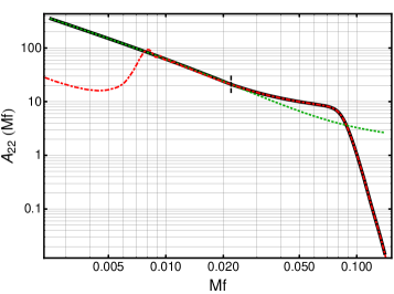
(see Arun et al. (2009)) with data of numerical simulations in full general relativity. The result in the equal-mass case can be seen in Fig. 2. Note that the transfer to the Fourier domain is completed by using (17) in (13) in combination with (15).
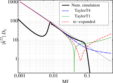
All variants of the 3PN Fourier amplitude agree reasonably well with the numerical relativity data roughly up to the frequency of the last stable circular orbit in the Schwarzschild limit, . Due to a comparable behavior even beyond this point we choose to construct the Fourier amplitude of our post-Newtonian model by using the TaylorT4 (9). The same choice was employed e.g. in Read et al. (2009).
IV Matching post-Newtonian and numerical relativity waveforms
IV.1 Basic notions
The basic criteria for evaluating the goodness of fit for the hybrid waveform require a notion of distance between two GW signals and . The simplest notion is the distance in the least-squares sense over an interval Ajith et al. (2007, 2008); Ajith (2008)
| (19) |
This can be used for the numerical relativity and the post-Newtonian waveform , with the interval being chosen so that both waveforms are reasonably good approximations (in a sense to be quantified later). Thus, the PN waveform is taken up to and the NR waveform is taken to start at , and they overlap within the interval .
Let us consider the frequency domain equivalent. Our convention for the Fourier transform of a signal is
| (20) |
One needs to be careful in converting the time interval to a frequency interval . In principle, the Fourier transform is “global” in time; signals that have compact support in time cannot have compact support in frequency, and vice versa. However, for the binary black hole waveforms (prior to the ring-down stage) that we are considering, the frequency always increases in time, so that we can sensibly associate a frequency interval with a given time interval . For these waveforms, we can consider the above distance definition in the frequency domain:
| (21) |
We shall use such a norm (applied to the phase) for constructing the hybrid waveform.
When evaluating the goodness of a hybrid waveform for a particular detector, we need to consider detector-specific inner products, which are convenient to describe in the frequency domain. Let be the single-sided power spectral density of the noise in a GW detector defined as
| (22) |
Here is the detector noise time series with its Fourier transform, ∗ denotes complex conjugation and refers to the expectation value over an ensemble of independent realizations of the noise, which is assumed to be a zero-mean, stationary, stochastic process. This equation implies that data at different frequencies are independent, and is one of the reasons why working in the frequency domain is so useful in data analysis. The time domain description of the noise is more complicated; and are in general not independent; is generally non-zero. For stationary noise this is a function only of , and is related to via a Fourier transform (see e.g. Papoulis and Unnikrishna Pillai (2002)).
Given , we use the following definition of an inner product between two signals and
| (23) |
where are the Fourier transforms of respectively. This inner product is appropriate for Gaussian noise and forms the basis for matched filtering (see e.g. Helstrom (1995)). It can be used to define a suitable notion of distance between two signals and as , where .
The distinguishability between and in the presence of noise can be understood with the following construction. Following Lindblom et al. (2008), we define a 1-parameter family of waveforms which interpolates linearly between and as
| (24) |
We obviously have and . The question of distinguishability between and now becomes one of estimating the value of [for the extended signal model ] in the presence of noise. If we use an unbiased estimator for , the variance of the estimator is bounded from below by the Cramer-Rao bound (see e.g. Stuart et al. (2009))
| (25) |
This can be a useful bound for large SNRs, which is in fact what we are interested in here; it is easier to distinguish between two loud waveforms and demands on the waveform model are correspondingly more stringent. Thus, a useful condition for being able to distinguish between the two waveforms is . If is the true waveform and our approximation to it, then we say that is a sufficiently accurate approximation if . Assuming that , it is clear that where is the optimal SNR. Hence, as we just remarked, the two signals are easier to distinguish when the detector is more sensitive, or when the signal amplitude is larger. It will be convenient to normalize the norm of and write this distinguishability criterion as
| (26) |
Thus, for a given detector, we choose a reasonable guess for the largest expected SNR and we compute the normalized distance between the two waveforms . If this exceeds , then we consider that the detector is able to distinguish between the two waveforms.
If we are interested in the less stringent requirement of detection rather than in strict distinguishability, then a sufficient condition is Lindblom et al. (2008)
| (27) |
where is the maximum tolerated fractional loss in SNR. More explicitly: if is the exact waveform and an approximation thereof, then the approximation is potentially useful for detection purposes if (27) is satisfied for an appropriate choice of . If we are willing to accept e.g. a 10% loss in detection rate, then a suitable choice is (corresponding to sources uniformly distributed in space). This value of does not take into account the additional loss in SNR due to discrete template banks used in realistic searches. In practice one might need to choose an order of magnitude smaller than this so that the total fractional loss in SNR remains acceptable. Since a more precise value is pipeline dependent, we shall ignore this caveat and use as a convenient reference; the reader can easily scale the results of this paper appropriately for different choices.
A useful way to describe the efficacy of approximate waveform models is through the concepts of effectualness and faithfulness introduced in Damour et al. (1998). Let be the exact waveform with parameters and the approximate waveform model be . The ambiguity function is defined as the normalized inner product maximized over extrinsic parameters
| (28) |
where is the time offset between the two waveforms, and is the initial phase. Performing a further maximization over the parameters of the model waveforms, we define . If exceeds a chosen threshold, e.g. 0.97, then the waveform model is said to be effectual. Effectual models are sufficient for detection. In order to be able to estimate parameters we also need the model to be faithful. This means that the value of which maximizes should not be biased too far away from .
IV.2 Issues in matching PN with NR
It is useful at this stage to discuss some of the issues that arise in combining PN and NR results. The discussion here will be short and incomplete, and the topic merits an in-depth investigation that is beyond the scope of the present work. Our immediate aim is simply to spell out some of the reasons why black hole parameters in the PN and NR frameworks may not necessarily refer to the same physical quantities. One should therefore not be surprised that when combining NR and PN waveforms, it might become necessary to vary the intrinsic black hole parameters as well. This is not to say that either PN or NR use incorrect definitions for black hole parameters, both frameworks are in fact consistent within their domains of applicability. The point rather is that the two formalisms are quite different when viewed as approximation schemes to general relativity, and these differences might need to be taken into account depending on the accuracy requirements for the matching.
Since PN and NR are both used to address the BBH problem, one could imagine starting with the two black holes very far apart, evolve them using appropriate PN equations of motion and compute the resulting waveforms. As one gets close to the merger, terminate the PN evolution and use this end-point to construct initial data for the full NR simulation which then evolves the black holes through the merger and ringdown. However, the formalisms and methods employed in the two cases are radically different and there are potential difficulties in carrying out this procedure.
The PN formalism is based on a perturbative expansion in powers of the small parameter , where is the orbital velocity and is the speed of light. In the usual formulations, PN theory uses a point-particle description of the black holes, and their parameters can be viewed as effective parameters which couple in the appropriate manner with the external background gravitational field (see e.g. Goldberger and Rothstein (2006); Porto and Rothstein (2008)). The goal of PN theory is to find a 1-parameter sequence of solutions to the field equations to any specified order in . It has recently been shown rigorously Oliynyk (2010) that, in the cosmological setting with gravitating perfect fluids, the 1-parameter family of solutions exists and admits an expansion in to any order. While similar results in the asymptotically-flat case are not yet available, it is certainly reassuring to know that PN works well in this non-trivial setting (in fact, it can be persuasively argued that the cosmological setting is more relevant to GW observations than strict asymptotic flatness). The errors in PN waveforms are then due to the systematic differences between the true waveform and the asymptotic series expansion in truncated at a finite order, and this error depends on which particular PN expansion one chooses to use.
In contrast, numerical relativity is based on the 3+1 formulation of general relativity as an initial value problem, and one solves the resulting partial differential equations numerically. The GW signal is typically measured at a large, but finite, coordinate distance from the source, and encoded in , the frame-dependent outgoing transverse component of the Weyl tensor component. The data from multiple coordinate radii are extrapolated to asymptotic distances, or evaluated at null infinity in the case that characteristic extraction is used Reisswig et al. (2009, 2010). For a given physical configuration (choice of masses, spins, separation etc.), one specifies the initial data consisting of the spatial metric and extrinsic curvature of the initial spatial slice. The physical initial data parameters should be chosen to be as compatible as possible with the spacetime computed in the PN formalism, and significant progress has been made in this regard Husa et al. (2008); Walther et al. (2009).
The black holes here are not point particles but rather black hole horizons. The parameters of the black hole are often computed as integrals over the apparent horizon, and in most cases the parameters used in constructing the initial data are also useful approximations to the true ones. There are, however, possible systematic errors. For example, if we are using the quasi-local horizon definitions, an important requirement is that the horizon should locally be approximately axisymmetric. The methods for finding the approximate symmetry vectors have become increasingly accurate and reliable Dreyer et al. (2003); Jasiulek (2009); Beetle (2008); Harte (2008); Lovelace et al. (2008). However, it should be kept in mind that the assumption of approximate axisymmetry is expected to become increasingly worse closer to the merger. Furthermore, the very use of apparent horizons is gauge dependent; using a different time coordinate will lead to a different set of apparent horizons and possibly also different values of the parameters. In the inspiral phase when the horizons are sufficiently isolated this gauge issue is not expected to be a problem, but as we get closer to the merger (this has not yet been quantified), the variation in the parameters due to gauge choices could become significant Nielsen et al. (2010).
Let us elaborate a little more on the spin. Most post-Newtonian treatments are based on the equations of motion derived in Corinaldesi and Papapetrou (1952); Papapetrou (1951). The starting point is the spin tensor constructed from moments of the stress energy tensor . Since has potentially 6 non-zero independent components, the system for the 4 equations of motion is over-determined. One thus imposes the additional spin supplementary conditions such as or with being the 4-momentum and the 4-velocity. These different conditions lead to physically different equations of motion and trajectories Kyrian and Semerák (2007). On the other hand, for black holes in NR, a common method for evaluating spin employs the formalism of quasi-local horizons Ashtekar and Krishnan (2004). The final result for the magnitude of the horizon angular momentum is an integral over the apparent horizon :
| (29) |
where is the extrinsic curvature of the Cauchy slice, is a suitable approximate axial symmetry vector on Dreyer et al. (2003); Jasiulek (2009); Beetle (2008); Harte (2008); Lovelace et al. (2008), and is the area element on the apparent horizon. The direction of the spin is harder to find, but some approximate methods are available Campanelli et al. (2007); Jasiulek (2009). There is yet no detailed study of possible analogs of the spin supplementary conditions in this formalism, or on the equations of motion for horizons with a given set of multipole moments. For a horizon with area and spin magnitude , the mass is given by the Christodoulou formula
| (30) |
Hence, uncertainties in spin can also lead to uncertainties in the mass.
As long as we are dealing with just the numerical or PN waveforms by themselves, these small effects in the definitions of mass and spin are not important for most applications. In fact, we can treat them as just convenient parameterizations of the waveform without worrying about their detailed physical interpretation. However, when we wish to compare the results from frameworks as different as PN and NR this may no longer work. Depending on the details of the matching procedure, systematic differences between the various definitions might need to be taken into account, or at the very least they should be quantified. If a particular case requires matching a very long PN portion (depending on the total mass and the lower-frequency cutoff of a particular detector), then even a small change in the PN parameters at the matching frequency can translate into a large phase difference at lower frequencies. One valid approach is to not assume a priori that the PN and NR parameters are equal to each other but rather, for a given numerical waveform, we search over PN waveforms in a particular PN approximant and find the best fit values. Finally, given that the NR and PN parts have different values of physical parameters, it is a matter of convention what values are to be assigned to the hybrid. The values of the parameters in the early inspiral are a convenient and astrophysically relevant choice.
IV.3 An illustration for non-spinning systems
Let us now move to a concrete case of constructing hybrid waveforms, considering the non-spinning Llama waveforms, i.e. data set #7 in Table 1. Recall that this data set consists of two waveforms with non-spinning black holes with mass ratios 1:1 (used in left and central panels of Fig. 6) and 1:2 (Figs. 3, 4, 5 and right panel of 6). Since these waveforms are calculated using the Llama code with extraction at future null-infinity with the Cauchy-characteristic method for the equal mass case, or well into the wave-zone for the 1:2 case, we are confident that systematic effects of waveform extraction are small. Even for these waveforms, based on the discussion above, in principle we should not rule out a small mismatch in the values of the spin (and perhaps also eccentricity) between the NR and PN waveforms. For simplicity, let us consider only the possibility that the symmetric mass ratio could be different, and restrict ourselves to non-spinning black holes and zero eccentricity. We would like to match the Llama waveforms with the frequency domain PN waveforms discussed in Sec. III with the values of the spins set to zero. The total mass sets the scale for the time (and frequency); in addition we have the extrinsic parameters for the time offset and initial phase and . Furthermore, we only consider the mode, so that the PN waveform is of the form in the frequency domain.
IV.3.1 Fitting errors
For a given NR waveform we consider a time window or, alternatively, in the frequency domain the matching region consists of a lower starting frequency and a width . We match the two waveforms in a least-squares sense by minimizing the phase difference in Fourier space
| (31) |
We optimize over all allowed time and phase shifts, i.e. , and the PN intrinsic parameters . Given the previous discussion on the possible differences between the intrinsic parameters in the PN and NR frameworks, here we have distinguished between the intrinsic parameter (5) appearing in and . Note that we are not only neglecting spins and eccentricity but also assume . Future analyses should successively drop these simplifications.
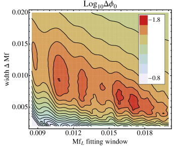
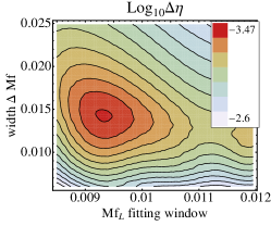
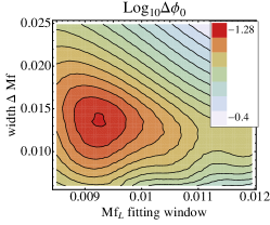
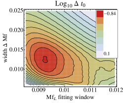
Let us now consider the choice of the optimal matching window , and the best fit values of . For each window, the least squares procedure gives a best fit value and 1- error estimates . Our principle for choosing is to pick the one for which the quality of fit between the NR and PN waveforms is the best, i.e. to minimize the fitting errors.
We first fix , choosing the 1:2 waveform, and consider fitting for . The result for is shown in Fig. 3 as a contour plot in the plane. There are clearly multiple best-fit islands but we already see that the optimal window choice turns out to be a long frequency width starting at low frequencies, or a relatively short window starting closer to the merger. Regarding the increasing error PN most likely introduces towards higher frequencies, we prefer using an early and long matching window. Though we do not show it here, the result is similar for the time offset .
It is more interesting instead to generalize this and allow all three parameters to vary. The main result is displayed in Fig. 4, which shows contour plots of the fitting errors , and in the plane. There are now clear and consistent minima for all errors and thus a clear best choice for and . At this optimal choice, we see that we can fit , and to better than , and , respectively. Apart from the error , the actual best fit value is also of great interest. Fig. 5 shows the value of as a function of the start frequency of the matching window and . The x-axis on this plot is the start point of the fitting window , and the color bar indicates . The most trustworthy values correspond to the optimal choice of obtained in Fig. 4; we indicate the union of all three minimal-error islands as a rectangle in Fig. 5.
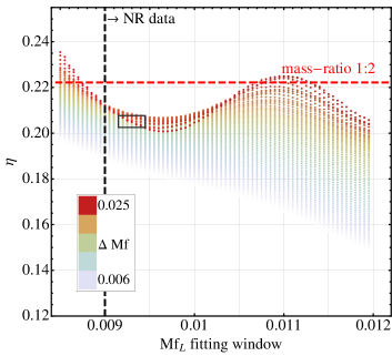
To summarize, from Figs. 4 and 5 we deduce that, if we were to ignore (the value that the numerical simulation nominally assumes) and simply try to find the best fit with the PN waveforms described in Sec. III, then we can clearly estimate the best matching region and a best fit value . This procedure illustrates a trade-off between trying to match at early frequencies, where our PN model is more reliable and having a sufficiently long fitting window, in which a considerable frequency evolution leads to an accurate estimate of the fitting parameters. The difference between and for this case is seen to be . This by itself does not say that the uncertainty in is because as we shall soon see, the uncertainties in the hybrid waveform are dominated by the uncertainties in the PN model. In other words, the NR waveform is closer to the true physical waveform within the matching window, and we should not actually use the best fit value of to construct the hybrid.
IV.3.2 Accuracy of the hybrid waveform
Later we shall show a phenomenological fit for the hybrid waveform and we shall claim that the fit reproduces the hybrid waveform sufficiently accurately. Here we first ask whether the hybrid waveform is itself sufficiently accurate subject to various errors. The basic criteria for evaluating this is the notion of a distance between two signals whose difference is , as given in Eq. (26). For two signals and , we shall consider the normalized distance squared , where is calculated from our best model (3PN amplitude, 3.5PN TaylorF2 phase combined with highest resolution NR waveform). Now the total mass becomes important. Previously, when we looked at the least square fits in Eq. (IV.3.1), the total mass appeared just as a scale factor. However, in the inner product Eq. (23), the power spectral density sets a frequency scale, and the value for becomes mass-dependent. We shall consider two design noise curves, Initial and Advanced LIGO Abadie et al. (2010); adv . We are then addressing the question of how different our hybrids would be if we were to use a slightly different result on either the NR or PN side.
On the NR side, we first consider data computed at different resolutions. The Llama waveforms for the equal-mass case have been computed at low, medium and high resolutions corresponding to spacing h = 0.96, 0.80 and 0.64 on the wave extraction grid. The finest grid, i.e. the grid covering the black hole, has a resolution of for the finest resolution. This is scaled by and for the medium and low resolution runs respectively. We combine these waveforms with the TaylorF2 model from Sec. III by using the optimal matching window discussed around Fig. 3 and . The result is shown in the left panel of Fig. 6. Hybrids constructed with medium- and high-resolution waveforms would be indistinguishable even with Advanced LIGO at a SNR of 80 over the considered mass range. Thus, we conclude that the numerical errors related to a finite resolution are not relevant in the hybrid construction process.
The uncertainties increase when comparing NR data produced by different codes. Similar to the analysis of different resolutions we calculate the distance of hybrid waveforms for non-spinning black holes with mass ratio 1:1 and 1:2. Results from data set #1 and #8 (see Table 1) were used, and the distance plot in the central panel of Fig. 6 shows that the 1:2 waveform would be distinguishable for Advanced LIGO at SNR 20 for a total masses between and . Note that these errors are dominated by our matching to PN which possibly yields different fit parameters for the PN model and therefore amplifies small differences in the NR data. Towards higher masses, the influence of this matching decreases as well as the distance of both waveform. However, as we shall show next, all these errors are still small compared to the intrinsic uncertainties introduced by PN and they do not matter for Initial LIGO. If we care only about detection with a minimal match see Eq. (27), we have even less to worry about.
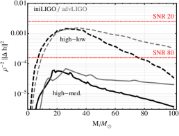
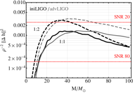
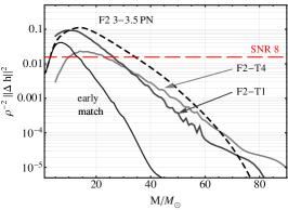
The errors on the PN side turn out to be much more important. The right panel of Fig. 6 illustrates the effect of using different PN approximants combined with the same SpEC equal mass simulation. We first use the fitting window discussed above, although the exceptionally long SpEC waveform would allow a much earlier matching. The dashed curve shows the difference in the hybrid waveforms when we match the 3PN or 3.5PN phase following the TaylorF2 frequency domain approximants described in Sec. III (the amplitude is taken at 3PN order in both cases). We see that the difference between these hybrids becomes significant even for Initial LIGO at SNR of 8 between a total mass of and . Similarly, the differences between the F2 and Taylor T1 & T4 approximants are also significant. For detection with see Eq. (27), we need to look at the horizontal line with in the right panel of Fig. 6. Both in the 3PN/3.5PN distance (dashed line) and the TaylorT1/TaylorF2 comparison (upper black solid line), there is a small range of masses for which the difference between the hybrids would matter even for detection.
As a reference, we make use of the fact that the numerical data #9 (Table 1) actually contains physical information to frequencies considerably smaller than the matching window used for our hybrid production. We therefore match the TaylorF2 phase at 3PN and 3.5PN order also with a much earlier fitting window (roughly a factor of lower in frequency). The right panel of Fig. 6 shows that the difference indicated as “early match” remains undetectable for a larger range of total masses. Expanding such studies may be used to quantify the necessary length of NR waveforms and estimate to which frequency standard PN results can be used in hybrid waveform constructions.
Having carried out this study of errors for non-spinning waveforms, we can now draw some conclusions for the aligned-spin case. In principle, the procedure outlined here remains valid; we should search over not only , but now also over the spins . We would not expect the results to be better than shown here for non-spinning waveforms because (i) we are adding two more parameters and (ii) the waveforms #1-4 are expected to have more wave-extraction systematic errors than the Llama results considered here. Most importantly, as we have just seen, the intrinsic errors in PN are more significant whereas the numerical accuracy is not the bottleneck. The intrinsic parameter biases in PN also show up when different PN models are compared with each other. An extensive comparison of different PN models is made in Buonanno et al. (2009); this paper quantifies the mutual effectualness and faithfulness of the different PN models and shows that errors of are not uncommon for Advanced LIGO. The less than 10% discrepancy in shown in Fig. 5 is thus entirely consistent with the differences between different PN models. To address this, one needs either improved PN models or a greater variety of longer NR waveforms such as the long SpEC simulation.
As a simplification, in what follows below we will choose the matching window based on maximizing over the extrinsic parameters motivated by Fig. 3. In that figure, we observe the best fit region extending diagonally from on the y-axis, to the bottom right corner. It turns out that for this diagonal, the upper frequency of the window does not vary much, , and we shall use this fact below for constructing hybrid waveforms for aligned spinning systems.
IV.4 Construction of hybrid waveforms for aligned spinning systems
Let us now proceed to the construction of a hybrid waveform model for non-precessing, spinning systems with comparable mass. Again, the waveforms described in Sec. III will be the basis for our model at low frequencies corresponding to the inspiral stage. On the other hand, the NR simulations described as data-sets #1–3 in Table 1 contain physical information for frequencies above . We will refer to Fig. 3 to justify our choice of an overlapping window at .
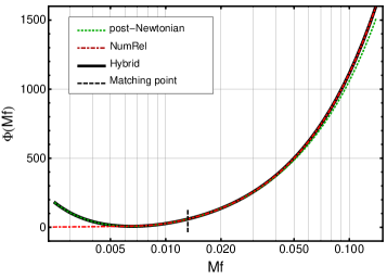
Once this interval is fixed, we now carry out the following matching procedure for all NR simulations of data-sets #1–3: PN and NR phases are aligned by fitting the free parameters and in Eq. (16); with a standard root-finding algorithm (starting at the mid point of the fitting interval) we find a frequency where PN and NR phase coincide and construct the hybrid phase consisting of TaylorF2 at and NR data at . An analogous procedure is applied to the amplitude, but in this case there is no freedom for adjusting any parameters. Hence, we use an educated guess for the matching frequency (compatible with that for the phase) and find the root where the difference of PN and NR amplitude vanishes. The hybrid amplitude consists of PN data before and NR data after . Small wiggles in the NR amplitude, due to the Fourier transform, do not affect the phenomenological fit significantly. The most important ingredient for arriving at an effectual model is the phase.
Fig. 7 illustrates the above-described hybrid construction method for matching PN and NR data in the frequency domain. The procedure does not require any re-sizing the PN or NR data and allows for the construction of waveforms containing all the information from the TaylorF2 approximant at low frequencies and input from the NR simulations for the late inspiral, merger and ringdown. The resulting hybrid PN-NR data cover a part of the parameter space corresponding to equal-valued, (anti-)aligned spins for and constitute the “target”waveforms to be fitted by the analytical phenomenological model described in Section V.
V Phenomenological model
In this section we present the phenomenological model developed in order to fit the hybrid PN-NR waveforms of Section IV to an analytical formula. A geometric description of the procedure for constructing phenomenological waveforms parametrized by just the physical parameters is detailed in Ajith et al. (2008), and here we just summarize it. Let be the space of intrinsic physical parameters that we are interested in. In the present case, this is the four-dimensional space of the component masses and spins . For each point in , let be the true physical waveform that we wish to approximate; in particular we consider only the dominant mode in this paper. Furthermore, as in Ajith et al. (2009), we model the spin effects using a single parameter defined as
| (32) |
where . As mentioned in Sec. II, this is justified from PN treatments of the inspiral Vaishnav et al. (2007) and from numerical simulations of the merger Reisswig et al. (2009) which considers equal mass systems. In these works, it is found that the dominant spin effect on the waveform is from the mass-weighted total spin of the system. On the PN side, this can be further justified by looking at the expressions for the PN phase and amplitudes given in the appendix [Eqs. (49,50)]. Consider the phase and amplitude terms as polynomials in and retain only the terms. At this lowest order, the amplitude and phase are seen to depend only on . We can therefore hope that this single parameter captures the main effects of the black hole spins, at least for the purpose of constructing an effectual model. In fact, whenever we incorporate pure PN contributions in our final model, we use them with . It is however important to note that this is only an approximation; while it suffices for our purposes (i.e., in constructing an effectual model) it will need to be refined as more faithful models are required. The degeneracy in the space of aligned spins will be studied in greater detail in a forthcoming paper Ohme , but here we look to construct a phenomenological model using only as the physical parameters.
We start with some known signals in this parameter space at points . We take these known signals to be the hybrid waveforms whose construction we described earlier. Here the NR waveforms are the BAM waveforms of data sets #1-3 summarized in Table 1, and the PN model is the 3.5PN frequency domain model for aligned spins described in Sec. III. Given the finite set of hybrid waveforms constructed from these ingredients, we wish to propose a phenomenological model that interpolates between the hybrid waveforms with sufficient accuracy. In constructing this phenomenological model, it is convenient to work not with the physical parameters , but rather with a larger set of phenomenological parameters , which we shall shortly describe. If is the space of phenomenological parameters, then we need to find a one-to-one mapping denoted , and thus the subspace of corresponding to the physical parameters. As the end result of this construction, for every physical parameter , we will know the corresponding phenomenological parameter and thus the corresponding phenomenological waveform .
Following the construction procedure of Section IV.4, we split our waveforms in amplitude and phase, both of which shall be fitted to a phenomenological model
| (33) |
For both the amplitude and the phase of the dominant mode of the GW radiation, we make use of the insights from PN and perturbation theory for the description of the inspiral and ringdown of the BBH coalescence, respectively, and introduce a phenomenological model to complete the description of the waveforms in the merger.
V.1 Phase model
The PN approach for the GW radiation based on the stationary phase approximation, introduced in Eq. (16) of Section III (used with and ), gives an adequate representation of the phase of the dominant mode during the adiabatic inspiral stage of the BBH coalescence . As the system transitions towards the merger phase, it is expected that further terms in the expansion are required to capture the features of the evolution. With this ansatz in mind, we propose a pre-merger phase of the form
| (34) |
where the coefficients are inspired by the SPA phase, redefined and phenomenologically fitted to agree with the hybrid waveforms in the region between the frequencies and , which depend on the spins and masses of the black holes in the form explained below in Eq. (36). Note that roughly corresponds to the starting frequency of our NR simulations.
As for the post-merger phase, the Teukolsky equation Teukolsky (1973) describes the ringdown of a slightly distorted spinning black hole. The metric perturbation for the fundamental mode at large distances can be expressed as an exponential damped sinusoidal
| (35) |
where is the mass of the ringing black hole, the distance from the source, and and correspond to the quality factor of the ringing down and the central frequency of the quasi-normal mode. These can be approximated with an error in the range by the following fit Berti et al. (2006)
| (36) | ||||
| (37) |
where and , as given in Table VIII of Berti et al. (2006) for the mode. The review Berti et al. (2009) presents a full description of quasi-normal modes. The quantity is the spin magnitude of the final black hole after the binary has merged, which can be inferred from the spins of the two black holes. In our case, we use the fit presented in Rezzolla et al. (2008), which maps the mass-ratio and spins of the binary to the total spin of the final black hole.
The analytical treatment of the ringdown (35) motivates a linear ansatz for the post-merger phase of the form
| (38) |
The parameters are not fitted, but obtained from the pre-merger ansatz (34) by taking the value and slope of the phase at the transition point . The transition between the different regimes is smoothened by means of tanh-window functions
| (39) |
to produce the final phenomenological phase
| (40) |
with , ; here we have used in the window functions . Roughly, these two transition points respectively signal the frequencies at which our NR simulations start and the point at which the binary merges, and have been found to provide the best match between the hybrids and the phenomenological model.
V.2 Amplitude model
In a similar manner to the phase, we approach the problem of fitting the amplitude of the GW by noting that the PN amplitude obtained from the SPA expression could be formally re-expanded as
| (41) |
where . We introduce a higher-order term to model the pre-merger amplitude
| (42) |
where the coefficient is introduced to model the amplitude in the pre-merger regime and is the amplitude constructed in Sec. III (see Fig. 2).
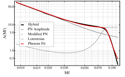
The ansatz for the amplitude during the ringdown is
| (43) |
where only the width and overall magnitude of the Lorentzian function are fitted to the hybrid data. The factor is introduced to correct the Lorentzian at high frequencies, since the hybrid data shows a faster fall-off, and accounts for the overall amplitude scale of the ringdown. In principle, the phenomenological parameter should not be necessary because the width of the Lorentzian for the ringdown should be given by the quality factor which depends only on the spin of the final black hole. However, recall that here we estimate the final spin from the initial configuration using the fit given in Rezzolla et al. (2008); accounts for the errors in this fit.
The phenomenological amplitude is constructed from these two pieces in a manner analogous to the phase
| (44) |
with and . Fig. 8 demonstrates how this phenomenological ansatz fits the hybrid amplitude in a smooth manner through the late inspiral, merger and ringdown.
V.3 Mapping the phenomenological coefficients
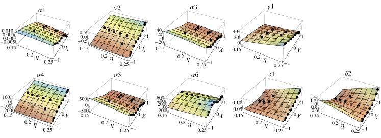
Our models for the amplitude and phase involve 9 phenomenological parameters defined in Eqs. (34), (42) and (43). The coefficients from (38) can be trivially derived from the set of . We now need to find the mapping from the physical to these phenomenological parameters. As mentioned earlier, instead of , we consider , the weighted sum of the spins, defined in Eq. (32). Thus, our phenomenological waveforms are parametrized only by the symmetric mass ratio and the spin parameter , as well as by the total mass of the system through a trivial rescaling. Fig. 9 shows the mapping of , and to surfaces in the –plane.
The 9 phenomenological coefficients introduced in our model, denoted generically by , are expressed in terms of the physical parameters of the binary as
| (45) |
which yields 5 coefficients for each of the 9 parameters, as given in table 2.
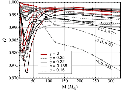
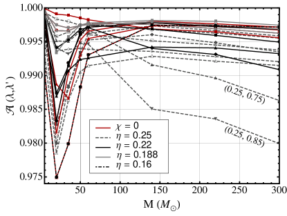
We evaluate the goodness of fit between the phenomenological model and the hybrid waveforms in terms of the fitting factor, i.e. the ambiguity function defined in Eq. (28) and the overlap, i.e. . In evaluating the overlap, we maximize over the extrinsic parameters as indicated in Eq. (28), but for the results shown in the upper panel of Fig. 10 we do not perform the additional maximization over the model parameters . Thus, the results shown there can be viewed as a lower bound on the effectualness. The maximization over the intrinsic parameters and allows to study the faithfulness of the model.
Figs. 10 and 11 illustrate the result using the design curve of the Advanced LIGO detector. Fig. 10 shows the overlap and fitting factor between the hybrid waveforms constructed in Sec. IV.4 and their corresponding phenomenological fit. The match approaches unity by construction at low masses and degrades with increasing total mass. Nevertheless, for none of the hybrid waveforms employed in the construction of our model does the overlap fall below a value of , thus reflecting the fact that the phenomenological model effectually represents the target signals. A further maximization over the parameters, shown in the lower panel of Fig. 10, indicates a maximum bias on the intrinsic parameters of the binary of .
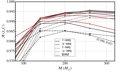
We have constructed a gravitational waveform model for binary black hole inspiral and coalescence starting with a particular set of simulations, and using a particular ansatz for the waveform. Is this model robust, and is it consistent with waveforms from other numerical simulations? In the upper panel of Fig. 11, and as a further test to assess the robustness of our model, we compute the maximized overlap between the phenomenological waveforms and the NR data-sets #4-7 that were not used in the construction of the model. At low masses, there is no contribution of these short NR waveforms in the frequency band of interest for Advanced LIGO, and it turns out that the overlaps can be computed only for .
In Fig. 11 we see that the maximization of the overlaps with respect to and shows values for all configurations; in this case the maximum bias in the parameters is . This is roughly consistent with Fig. 10 which shows the overlap and fitting factor of the model with the original set of hybrid waveforms. These results prove that our model is effectual and, thus, sufficient for detection. We shall study its effectualness and faithfulness in greater detail in a forthcoming paper.
VI Summary and future work
The aim of this paper has been to construct an analytical model for the inspiral and coalescence of binary black hole systems with aligned spins and comparable masses in circular orbits. Since this requires merging post-Newtonian and numerical relativity waveforms, one of the main themes has been to quantify the internal consistency of hybrid waveforms. This is important because even if one succeeds in finding a useful fit for a family of hybrid waveforms, one still needs to show that the hybrid one started with is a sufficiently good approximation to the true physical waveforms. We investigated the systematics of constructing hybrid waveforms for accurate non-spinning waveforms based on the Llama code and we saw that neither the numerical errors nor the hybrid-construction errors are significant. This suggests that in order to improve the accuracy of hybrid waveforms, we require either longer NR waveforms so that the matching with PN can be done earlier in the inspiral phase, or improved PN models that are more accurate at frequencies closer to the binary merger.
With the hybrid waveforms for non-precessing systems in hand, we constructed an analytical model for the waveform which has an overlap and fitting factor of better than 97% for Advanced LIGO with the hybrid waveforms for systems with a total mass ranging up to . Since these overlaps are comparable to those achieved with the alternative phenomenological waveform construction presented in Ajith et al. (2009), we conclude that this process is robust, and, in particular, its accuracy is not affected by the way in which the transitions between inspiral, merger and ringdown are modeled. Furthermore, though we have not discussed it in detail in this paper, it turns out that the model presented here agrees very well with the model of Ajith et al. (2009). This will be discussed in detail in a forthcoming paper Ohme
In the future we will study in greater detail the effectualness and faithfulness of this waveform model, thereby quantifying more precisely its performance for detection and parameter estimation. In this context it is important to extend this work to modes higher than the dominant , spherical harmonics. It was shown recently McWilliams et al. (2010) that the overlap with the real signal can possibly be affected by the inclusion of higher modes up to the order of , which is comparable or greater than the disagreement we find between hybrid and phenomenological model.
We will further quantify the behavior of our templates in real non-Gaussian detector noise, and use them in real searches for gravitational wave signals. Eventually, work is underway in extending the model to include precessing spins. Our phenomenological model can be readily applied to existent GW detection efforts within the LIGO/Virgo Scientific Collaborations. Ongoing searches are already making use of inspiral-merger-ringdown waveforms, such as the EOBNR family and the phenomenological family of Ajith et al. (2007, 2008); Ajith (2008); Ajith et al. (2009) in the form of software injections and as filter approximants. Our newly developed frequency-domain matching procedure should serve to cross-check the validity of these alternative approaches and to complement them.
Acknowledgments
We thank Doreen Müller for carrying out some of the BAM simulations, and Stas Babak, Vitor Cardoso, Steve Fairhurst, Ian Hinder, Doreen Müller, Dirk Pützfeld, Bangalore Sathyaprakash and Bernard Schutz for useful comments and discussions. LS has been partially supported by DAAD grant A/06/12630. MH was supported by FWF Lise-Meitner project M1178-N16 at the University of Vienna. SH was supported by DAAD grant D/07/13385 and grant FPA-2007-60220 from the Spanish Ministry of Science. DP has been supported by grant CSD-2007-00042 of the Spanish Ministry of Science. DP and CR received support from the Bundesministerium für Bildung und Forschung, Germany. BAM simulations were performed at computer centers LRZ Munich, ICHEC Dublin, VSC Vienna, CESGA Santiago the Compostela and at MareNostrum at Barcelona Supercomputing Center – Centro Nacional de Supercomputación (Spanish National Supercomputing Center). This work was supported in part by the DFG grant SFB/Transregio 7 “Gravitational wave astronomy” and by the DLR (Deutsches Zentrum für Luft- und Raumfahrttechnik).
Appendix A PN expansion coefficients
For the convenience of the reader we explicitly give all the PN expansion coefficients used in Section III as functions of the symmetric mass ratio (5), the dimensionless spin magnitudes , where is the unit angular momentum vector, and . The energy (6) is given in terms of
| (46) | ||||
The flux coefficients read
| (47) | ||||
is the Euler constant. Note that the next-to-leading order spin-orbit effects appearing at relative 2.5PN order () have recently been corrected Blanchet et al. (2010) and we take these corrections into account.
The TaylorT4 approximant can be written as a series (9) with the following coefficients
| (48) | ||||
The spin-dependent terms that appear at 3 and 3.5 PN order (i.e., in and ) are not complete since the corresponding terms are not known in energy and flux. However, in this re-expansion they do appear as contributions from lower order spin effects and we keep them.
The TaylorF2 description of the Fourier phase (16) is expressed in terms of
| (49) | ||||
The comment we just made about the spin contributions at 3 and 3.5 PN order holds for the -coefficients of the TaylorF2 phase as well. Also, note that the contributions in that are not proportional to could be absorbed in a re-definition of the undetermined additional phase that appears in Eq. (16). (A similar discussion can be found in Arun et al. (2005).) However, since we chose to set when combining this phase description with other analytical formulas in our phenomenological model (40), it is important to keep all terms in .
References
- Abbott et al. (2009) B. Abbott et al. (LIGO Scientific), Rept. Prog. Phys., 72, 076901 (2009a), arXiv:0711.3041 [gr-qc] .
- Acernese et al. (2008) F. Acernese et al., Class. Quant. Grav., 25, 184001 (2008).
- Grote (2008) H. Grote (LIGO Scientific), Class. Quant. Grav., 25, 114043 (2008).
- Shaddock (2009) D. A. Shaddock, Publ. Astron. Soc. Austral., 26, 128 (2009), arXiv:0909.0650 [gr-qc] .
- Punturo et al. (2010) M. Punturo et al., Class. and Quant. Grav., 27, 084007 (2010).
- Pretorius (2005) F. Pretorius, Phys. Rev. Lett., 95, 121101 (2005a), arXiv:gr-qc/0507014 .
- Campanelli et al. (2006) M. Campanelli, C. O. Lousto, P. Marronetti, and Y. Zlochower, Phys. Rev. Lett., 96, 111101 (2006), arXiv:gr-qc/0511048 .
- Baker et al. (2006) J. G. Baker, J. Centrella, D.-I. Choi, M. Koppitz, and J. van Meter, Phys. Rev. Lett., 96, 111102 (2006a), arXiv:gr-qc/0511103 .
- Hannam (2009) M. Hannam, Class. Quant. Grav., 26, 114001 (2009), arXiv:0901.2931 [gr-qc] .
- (10) “Numerial INJection Analysis project,” http://www.ninja-project.org.
- Hinder (2010) I. Hinder, Class. Quant. Grav., 27, 114004 (2010), arXiv:1001.5161 [gr-qc] .
- Hannam et al. (2009) M. Hannam et al., Phys. Rev., D79, 084025 (2009), arXiv:0901.2437 [gr-qc] .
- Aylott et al. (2009) B. Aylott et al., Class. Quant. Grav., 26, 165008 (2009a), arXiv:0901.4399 [gr-qc] .
- Aylott et al. (2009) B. Aylott et al., Class. Quant. Grav., 26, 114008 (2009b), arXiv:0905.4227 [gr-qc] .
- Scheel et al. (2009) M. A. Scheel et al., Phys. Rev., D79, 024003 (2009), arXiv:0810.1767 [gr-qc] .
- Buonanno et al. (2007) A. Buonanno, G. B. Cook, and F. Pretorius, Phys. Rev., D75, 124018 (2007a), arXiv:gr-qc/0610122 .
- Baker et al. (2007) J. G. Baker, J. R. van Meter, S. T. McWilliams, J. Centrella, and B. J. Kelly, Phys. Rev. Lett., 99, 181101 (2007), arXiv:gr-qc/0612024 .
- Hannam et al. (2008) M. Hannam, S. Husa, U. Sperhake, B. Bruegmann, and J. A. González, Phys. Rev., D77, 044020 (2008a), arXiv:0706.1305 [gr-qc] .
- Gopakumar et al. (2008) A. Gopakumar, M. Hannam, S. Husa, and B. Brügmann, Phys. Rev., D78, 064026 (2008), arXiv:0712.3737 [gr-qc] .
- Boyle et al. (2007) M. Boyle et al., Phys. Rev., D76, 124038 (2007), arXiv:0710.0158 [gr-qc] .
- Boyle et al. (2008) M. Boyle et al., Phys. Rev., D78, 104020 (2008), arXiv:0804.4184 [gr-qc] .
- Hinder et al. (2008) I. Hinder, F. Herrmann, P. Laguna, and D. Shoemaker, (2008), arXiv:0806.1037 [gr-qc] .
- Hannam et al. (2008) M. Hannam, S. Husa, B. Brügmann, and A. Gopakumar, Phys. Rev., D78, 104007 (2008b), arXiv:0712.3787 [gr-qc] .
- Campanelli et al. (2009) M. Campanelli, C. O. Lousto, H. Nakano, and Y. Zlochower, Phys. Rev., D79, 084010 (2009), arXiv:0808.0713 [gr-qc] .
- Berti et al. (2007) E. Berti et al., Phys. Rev., D76, 064034 (2007), arXiv:gr-qc/0703053 .
- Berti et al. (2008) E. Berti, V. Cardoso, J. A. González, U. Sperhake, and B. Brügmann, Class. Quant. Grav., 25, 114035 (2008), arXiv:0711.1097 [gr-qc] .
- Buonanno and Damour (1999) A. Buonanno and T. Damour, Phys. Rev., D59, 084006 (1999), arXiv:gr-qc/9811091 .
- Buonanno and Damour (2000) A. Buonanno and T. Damour, Phys. Rev., D62, 064015 (2000), arXiv:gr-qc/0001013 .
- Damour et al. (1998) T. Damour, B. R. Iyer, and B. S. Sathyaprakash, Phys. Rev., D57, 885 (1998a), arXiv:gr-qc/9708034 .
- Damour et al. (2000) T. Damour, P. Jaranowski, and G. Schäfer, Phys. Rev., D62, 084011 (2000), arXiv:gr-qc/0005034 .
- Buonanno et al. (2007) A. Buonanno et al., Phys. Rev., D76, 104049 (2007b), arXiv:0706.3732 [gr-qc] .
- Buonanno et al. (2009) A. Buonanno et al., Phys. Rev., D79, 124028 (2009a), arXiv:0902.0790 [gr-qc] .
- Damour et al. (2008) T. Damour, A. Nagar, E. N. Dorband, D. Pollney, and L. Rezzolla, Phys. Rev., D77, 084017 (2008a), arXiv:0712.3003 [gr-qc] .
- Damour et al. (2008) T. Damour, A. Nagar, M. Hannam, S. Husa, and B. Brügmann, Phys. Rev., D78, 044039 (2008b), arXiv:0803.3162 [gr-qc] .
- Damour and Nagar (2009) T. Damour and A. Nagar, Phys. Rev., D79, 081503 (2009), arXiv:0902.0136 [gr-qc] .
- Pan et al. (2010) Y. Pan et al., Phys. Rev., D81, 084041 (2010), arXiv:0912.3466 [gr-qc] .
- Ajith et al. (2007) P. Ajith et al., Class. Quant. Grav., 24, S689 (2007), arXiv:0704.3764 [gr-qc] .
- Ajith (2008) P. Ajith, Class. Quant. Grav., 25, 114033 (2008), arXiv:0712.0343 [gr-qc] .
- Ajith et al. (2008) P. Ajith et al., Phys. Rev., D77, 104017 (2008), arXiv:0710.2335 [gr-qc] .
- Ajith et al. (2009) P. Ajith et al., (2009), arXiv:0909.2867 [gr-qc] .
- Sturani et al. (2010) R. Sturani et al., (2010), arXiv:1005.0551 [gr-qc] .
- Apostolatos et al. (1994) T. A. Apostolatos, C. Cutler, G. J. Sussman, and K. S. Thorne, Phys. Rev., D49, 6274 (1994).
- Brügmann et al. (2008) B. Brügmann et al., Phys. Rev., D77, 024027 (2008a), arXiv:gr-qc/0610128 .
- Husa et al. (2008) S. Husa, M. Hannam, J. A. González, U. Sperhake, and B. Brügmann, Phys. Rev., D77, 044037 (2008a), arXiv:0706.0904 [gr-qc] .
- Pollney et al. (2007) D. Pollney, C. Reisswig, L. Rezzolla, B. Szilágyi, M. Ansorg, B. Deris, P. Diener, E. N. Dorband, M. Koppitz, A. Nagar, and E. Schnetter, Phys. Rev., D76, 124002 (2007), arXiv:0707.2559 [gr-qc] .
- Pollney et al. (2009) D. Pollney, C. Reisswig, E. Schnetter, N. Dorband, and P. Diener, (2009a), arXiv:0910.3803 [gr-qc] .
- Scheel et al. (2006) M. A. Scheel, H. P. Pfeiffer, L. Lindblom, L. E. Kidder, O. Rinne, and S. A. Teukolsky, Phys. Rev., D74, 104006 (2006), arXiv:gr-qc/0607056 .
- Abbott et al. (2008) B. Abbott et al. (LIGO Scientific), Phys. Rev., D77, 062002 (2008a), arXiv:0704.3368 [gr-qc] .
- Abbott et al. (2009) B. P. Abbott et al. (LIGO Scientific), Phys. Rev., D79, 122001 (2009b), arXiv:0901.0302 [gr-qc] .
- Abbott et al. (2009) B. P. Abbott et al. (LIGO Scientific), Phys. Rev., D80, 047101 (2009c), arXiv:0905.3710 [gr-qc] .
- Abbott et al. (2008) B. Abbott et al. (LIGO Scientific), Phys. Rev., D78, 042002 (2008b), arXiv:0712.2050 [gr-qc] .
- Van Den Broeck et al. (2009) C. Van Den Broeck et al., Phys. Rev., D80, 024009 (2009), arXiv:0904.1715 [gr-qc] .
- Vaishnav et al. (2007) B. Vaishnav, I. Hinder, F. Herrmann, and D. Shoemaker, Phys. Rev., D76, 084020 (2007), arXiv:0705.3829 [gr-qc] .
- Reisswig et al. (2009) C. Reisswig et al., Phys. Rev., D80, 124026 (2009a), arXiv:0907.0462 [gr-qc] .
- Hannam et al. (2010) M. Hannam, S. Husa, F. Ohme, D. Müller, and B. Brügmann, (2010), arXiv:1007.4789 [gr-qc] .
- Rezzolla et al. (2008) L. Rezzolla et al., Astrophys., J679, 1422 (2008a), arXiv:0708.3999 [gr-qc] .
- Rezzolla et al. (2008) L. Rezzolla et al., Astrophys. J., 674, L29 (2008b), arXiv:0710.3345 [gr-qc] .
- Chu et al. (2009) T. Chu, H. P. Pfeiffer, and M. A. Scheel, Phys. Rev., D80, 124051 (2009), arXiv:0909.1313 [gr-qc] .
- Baker et al. (2006) J. G. Baker, J. Centrella, D.-I. Choi, M. Koppitz, and J. van Meter, Phys. Rev. Lett., 96, 111102 (2006b), arXiv:gr-qc/0511103 .
- Pretorius (2005) F. Pretorius, Class. Quant. Grav., 22, 425 (2005b), arXiv:gr-qc/0407110 .
- Pollney et al. (2009) D. Pollney, C. Reisswig, N. Dorband, E. Schnetter, and P. Diener, Phys. Rev., D80, 121502 (2009b), arXiv:0910.3656 [gr-qc] .
- Brügmann et al. (2008) B. Brügmann, J. A. González, M. Hannam, S. Husa, and U. Sperhake, Phys. Rev., D77, 124047 (2008b), arXiv:0707.0135 [gr-qc] .
- Penrose and Rindler (1986) R. Penrose and W. Rindler, Spinors and Space-time: Two-spinor calculus and relativistic fields (Press Syndicate of the University of Cambridge, 1986).
- Regge and Wheeler (1957) T. Regge and J. A. Wheeler, Phys. Rev., 108, 1063 (1957).
- Zerilli (1970) F. J. Zerilli, Phys. Rev. Lett., 24, 737 (1970).
- Abrahams and Evans (1988) A. M. Abrahams and C. R. Evans, Phys. Rev., D37, 318 (1988).
- Abrahams and Evans (1990) A. M. Abrahams and C. R. Evans, Phys. Rev., D42, 2585 (1990).
- Reisswig et al. (2009) C. Reisswig, N. T. Bishop, D. Pollney, and B. Szilagyi, Phys. Rev. Lett., 103, 221101 (2009b), arXiv:0907.2637 [gr-qc] .
- Reisswig et al. (2010) C. Reisswig, N. T. Bishop, D. Pollney, and B. Szilagyi, Class. Quant. Grav., 27, 075014 (2010), arXiv:0912.1285 [gr-qc] .
- (70) Waveforms are available at http://www.black-holes.org/Waveforms.html.
- Blanchet (2006) L. Blanchet, Living Reviews in Relativity, 9 (2006), arXiv:gr-qc/0202016 .
- Damour et al. (2001) T. Damour, B. R. Iyer, and B. S. Sathyaprakash, Phys. Rev., D63, 044023 (2001a), arXiv:gr-qc/0010009 .
- Damour et al. (2002) T. Damour, B. R. Iyer, and B. S. Sathyaprakash, Phys. Rev., D66, 027502 (2002), arXiv:gr-qc/0207021 .
- Damour et al. (2005) T. Damour, B. R. Iyer, and B. S. Sathyaprakash, Phys. Rev., D72, 029901 (2005).
- Arun et al. (2005) K. G. Arun, B. R. Iyer, B. S. Sathyaprakash, and P. A. Sundararajan, Phys. Rev., D71, 084008 (2005), arXiv:gr-qc/0411146 .
- Blanchet et al. (2008) L. Blanchet, G. Faye, B. R. Iyer, and S. Sinha, Class. and Quant. Grav., 25, 165003 (2008), arXiv:0802.1249 [gr-qc] .
- Arun et al. (2009) K. G. Arun, A. Buonanno, G. Faye, and E. Ochsner, Phys. Rev., D79, 104023 (2009), arXiv:0810.5336 [gr-qc] .
- Damour et al. (2001) T. Damour, P. Jaranowski, and G. Schäfer, Phys. Lett., B513, 147 (2001b), arXiv:gr-qc/0105038 .
- Blanchet et al. (2004) L. Blanchet, T. Damour, G. Esposito-Farèse, and B. R. Iyer, Phys. Rev. Lett., 93, 091101 (2004), arXiv:gr-qc/0406012 .
- Buonanno et al. (2006) A. Buonanno, Y. Chen, and T. Damour, Phys. Rev., D74, 104005 (2006), arXiv:gr-qc/0508067 .
- Kidder (1995) L. E. Kidder, Phys. Rev., D52, 821 (1995), arXiv:gr-qc/9506022 .
- Blanchet et al. (2006) L. Blanchet, A. Buonanno, and G. Faye, Phys. Rev., D74, 104034 (2006), arXiv:gr-qc/0605140 .
- Damour (2001) T. Damour, Phys. Rev., D64, 124013 (2001), arXiv:gr-qc/0103018 .
- Poisson (1998) E. Poisson, Phys. Rev., D57, 5287 (1998), arXiv:gr-qc/9709032 .
- Faye et al. (2006) G. Faye, L. Blanchet, and A. Buonanno, Phys. Rev., D74, 104033 (2006), arXiv:gr-qc/0605139 .
- Alvi (2001) K. Alvi, Phys. Rev., D64, 104020 (2001), arXiv:gr-qc/0107080 .
- Buonanno et al. (2009) A. Buonanno, B. Iyer, E. Ochsner, Y. Pan, and B. S. Sathyaprakash, Phys. Rev., D80, 084043 (2009b), arXiv:0907.0700 [gr-qc] .
- Read et al. (2009) J. S. Read et al., Phys. Rev., D79, 124033 (2009), arXiv:0901.3258 [gr-qc] .
- Papoulis and Unnikrishna Pillai (2002) A. Papoulis and S. Unnikrishna Pillai, Probability, Random Variables and Stochastic Processes, 4th ed. (McGraw Hill Higher Education, 2002).
- Helstrom (1995) C. W. Helstrom, Elements of signal detection and estimation (Prentice-Hall, Inc., Upper Saddle River, NJ, USA, 1995) ISBN 0-13-808940-X.
- Lindblom et al. (2008) L. Lindblom, B. J. Owen, and D. A. Brown, Phys. Rev., D78, 124020 (2008), arXiv:0809.3844 [gr-qc] .
- Stuart et al. (2009) A. Stuart, K. Keith Ord, and S. Arnold, Kendall’s Advanced Theory of Statistics:Volume 2A -Classical Inference and and the Linear Model, 6th ed. (Wiley, 2009).
- Damour et al. (1998) T. Damour, B. R. Iyer, and B. S. Sathyaprakash, Phys. Rev., D57, 885 (1998b).
- Goldberger and Rothstein (2006) W. D. Goldberger and I. Z. Rothstein, Phys. Rev., D73, 104029 (2006), arXiv:hep-th/0409156 .
- Porto and Rothstein (2008) R. A. Porto and I. Z. Rothstein, Phys. Rev., D78, 044012 (2008), arXiv:0802.0720 [gr-qc] .
- Oliynyk (2010) T. A. Oliynyk, Commun. Math. Phys., 295, 431 (2010), arXiv:0908.2836 [gr-qc] .
- Husa et al. (2008) S. Husa, J. A. González, M. Hannam, B. Brügmann, and U. Sperhake, Class. Quant. Grav., 25, 105006 (2008b), arXiv:0706.0740 [gr-qc] .
- Walther et al. (2009) B. Walther, B. Brügmann, and D. Müller, Phys. Rev., D79, 124040 (2009), arXiv:0901.0993 [gr-qc] .
- Dreyer et al. (2003) O. Dreyer, B. Krishnan, D. Shoemaker, and E. Schnetter, Phys. Rev., D67, 024018 (2003), arXiv:gr-qc/0206008 .
- Jasiulek (2009) M. Jasiulek, Class. Quant. Grav., 26, 245008 (2009), arXiv:0906.1228 [gr-qc] .
- Beetle (2008) C. Beetle, (2008), arXiv:0808.1745 [gr-qc] .
- Harte (2008) A. I. Harte, Class. Quant. Grav., 25, 205008 (2008), arXiv:0805.4259 [gr-qc] .
- Lovelace et al. (2008) G. Lovelace, R. Owen, H. P. Pfeiffer, and T. Chu, Phys. Rev., D78, 084017 (2008), arXiv:0805.4192 [gr-qc] .
- Nielsen et al. (2010) A. B. Nielsen, M. Jasiulek, B. Krishnan, and E. Schnetter, (2010), arXiv:1007.2990 [gr-qc] .
- Corinaldesi and Papapetrou (1952) E. Corinaldesi and A. Papapetrou, Proc. Roy. Soc. Lond., A64, 259 (1952).
- Papapetrou (1951) A. Papapetrou, Proc. Roy. Soc. Lond., A209, 248 (1951).
- Kyrian and Semerák (2007) K. Kyrian and O. Semerák, Mon. Not. Roy. Astr. Soc., 382, 1922 (2007).
- Ashtekar and Krishnan (2004) A. Ashtekar and B. Krishnan, Living Rev. Rel., 7, 10 (2004), arXiv:gr-qc/0407042 .
- Campanelli et al. (2007) M. Campanelli, C. O. Lousto, Y. Zlochower, B. Krishnan, and D. Merritt, Phys. Rev., D75, 064030 (2007), arXiv:gr-qc/0612076 .
- Abadie et al. (2010) J. Abadie et al. (LIGO Scientific Collaboration and Virgo Collaboration), ArXiv e-prints (2010), 1003.2481, arXiv:1003.2481 .
- (111) “Advanced LIGO anticipated sensitivity curves,” "https://dcc.ligo.org/cgi-bin/DocDB/ShowDocument?docid=2974".
- (112) F. Ohme, In preparation.
- Teukolsky (1973) S. A. Teukolsky, Astrophys. J., 185, 635 (1973).
- Berti et al. (2006) E. Berti, V. Cardoso, and C. M. Will, Phys. Rev., D73, 064030 (2006), arXiv:gr-qc/0512160 .
- Berti et al. (2009) E. Berti, V. Cardoso, and A. O. Starinets, Class. Quant. Grav., 26, 163001 (2009), arXiv:0905.2975 [gr-qc] .
- McWilliams et al. (2010) S. T. McWilliams, B. J. Kelly, and J. G. Baker, (2010), arXiv:1004.0961 [gr-qc] .
- Blanchet et al. (2010) L. Blanchet, A. Buonanno, and G. Faye, Phys. Rev. D, 81, 089901 (2010), arXiv:gr-qc/0605140v4 .