Three-Point Correlation Functions of SDSS Galaxies: Luminosity and Color Dependence in Redshift and Projected Space

Abstract

The three-point correlation function (3PCF) provides an important view into the clustering of galaxies that is not available to its lower order cousin, the two-point correlation function (2PCF). Higher order statistics, such as the 3PCF, are necessary to probe the non-Gaussian structure and shape information expected in these distributions. We measure the clustering of spectroscopic galaxies in the Main Galaxy Sample of the Sloan Digital Sky Survey (SDSS), focusing on the shape or configuration dependence of the reduced 3PCF in both redshift and projected space. This work constitutes the largest number of galaxies ever used to investigate the reduced 3PCF, using over $220\,000$ galaxies in three volume-limited samples. We find significant configuration dependence of the reduced 3PCF at $3-27\;h^{-1}\mathrm{Mpc}$, in agreement with $\Lambda\mathrm{CDM}$ predictions and in disagreement with the hierarchical ansatz. Below $6\;h^{-1}\mathrm{Mpc}$, the redshift space reduced 3PCF shows a smaller amplitude and weak configuration dependence in comparison with projected measurements suggesting that redshift distortions, and not galaxy bias, can make the reduced 3PCF appear consistent with the hierarchical ansatz. The reduced 3PCF shows a weaker dependence on luminosity than the 2PCF, with no significant dependence on scales above $9\;h^{-1}\mathrm{Mpc}$. On scales less than $9\;h^{-1}\mathrm{Mpc}$, the reduced 3PCF appears more affected by galaxy color than luminosity. We demonstrate the extreme sensitivity of the 3PCF to systematic effects such as sky completeness and binning scheme, along with the difficulty of resolving the errors. Some comparable analyses make assumptions that do not consistently account for these effects.

1. Introduction

In the current paradigm of structure formation, an almost uniform distribution of mass at early times in the universe evolved through gravitational instability into the irregular and complex distribution that galaxies occupy today. Gravitational dynamics are sensitive to cosmology and depend on the spatial curvature of the universe as well as the nature of its contents. A combination of many observations including both constraints from large-scale structure (LSS; Tegmark et al. 2004; Cole et al. 2005; Eisenstein et al. 2005; Tegmark et al. 2006; Sánchez et al. 2009) and the cosmic microwave background (CMB; Spergel et al. 2007) support a standard model in accordance with current observations (see recent constraints in Komatsu et al. 2009). These observations suggest a critically dense (spatially flat) universe, consisting of a small amount of baryonic matter, several times more mass in cold dark matter (CDM), and well over the majority of the current energy density in some form of dark energy ($\Lambda$). This concordance model, referred to as $\Lambda\mathrm{CDM}$, forms the basis of predicting LSS and the framework underlying statistical studies of galaxy distributions.

Modern galaxy surveys, such as the Sloan Digital Sky Survey (SDSS; York et al. 2000; Stoughton et al. 2002), provide a wealth of information about large-scale structure, galaxy formation, galaxy evolution and cosmology. The main workhorse for statistical analyses has been the $n$-point correlation functions (Peebles 1980). The most common clustering measurements use the two-point correlation function (2PCF) or its analog in Fourier space, the power spectrum. Results from measurements of these statistics using observational datasets have been able to distinguish subtle differences in theoretical models of how galaxies occupy dark matter halos (e.g. departures from power law clustering, Zehavi et al. 2004), a comprehensive study of the effects of luminosity and color on galaxy clustering (Zehavi et al. 2005, 2010), as well as providing precise measurements of cosmological phenomena to better understand the nature of dark energy (e.g. baryon acoustic oscillations, Eisenstein et al. 2005).

If the galaxy distribution was entirely Gaussian, the 2PCF would provide a complete description of galaxy clustering. Although analyses of the CMB suggest that the primordial mass fluctuations in our universe appear extremely Gaussian (Komatsu et al. 2009), we expect gravitational collapse to produce non-Gaussian signatures in the galaxy distribution that we measure today (Bernardeau et al. 2002). As such, the 2PCF provides only a partial view of the full distribution and cannot sufficiently probe non-Gaussian signals.

To investigate non-Gaussian structure, as well as shape information in these distributions, we require higher order clustering statistics. In the hierarchy of $n$-point correlation functions, the 3PCF is the lowest order statistic to provide information on shape (Peebles 1980). For example, this enables probes of the triaxial nature of halos and extended filaments within the “cosmic web”. Measurements of higher order moments allow a more complete picture of the galaxy distribution, breaking model degeneracies describing cosmology and galaxy bias (Zheng and Weinberg 2007; Kulkarni et al. 2007).

The statistical strength of information in higher order moments of clustering can potentially rival that of the two-point statistics (Sefusatti and Scoccimarro 2005). As a complement to bispectrum (Fourier transform of the 3PCF) and redshift-space analyses, we can use the projected 3PCF to sidestep redshift distortions in observational data by integrating out the effect of peculiar velocities from the density field.

The additional information contained in higher order moments comes at a price. Their increased complexity make the measurements, modeling and interpretation difficult. Theoretically, non-linear contributions have significant non-trivial implications. Their calculation gets computationally challenging and efficient algorithms become critically important. They require larger and cleaner galaxy samples as they show more sensitivity to observational systematics than the 2PCF. As it was recently described: “the overlap between well understood theory and reliable measurements is in fact disquietingly small” (Szapudi 2009). This work attempts to increase this overlap by leveraging the massive dataset available from the SDSS.

Previous work has estimated the 3PCF from modern galaxy redshift surveys, including work on the the two-degree field galaxy redshift survey (Jing and Börner 2004; Wang et al. 2004; Gaztañaga et al. 2005) and results from earlier SDSS data (Kayo et al. 2004; Nichol et al. 2006; Kulkarni et al. 2007). Fourier space analogs or related higher order statistics have also been measured for these datasets (Verde et al. 2002; Pan and Szapudi 2005; Hikage et al. 2005; Nishimichi et al. 2007).

This work is the first of two papers analyzing the reduced 3PCF on SDSS galaxy samples, where this work focuses on details of the measurements as well as the dependence of clustering from varying the galaxy sample’s luminosity and color. The second paper (McBride, et al. 2010) utilizes the configuration dependence to constrain non-linear galaxy-mass bias parameters in the local bias model (Fry and Gaztanaga 1993). Throughout our study, we assume a standard flat $\Lambda\mathrm{CDM}$ cosmology where $\Omega_{\mathrm{m}}=0.3$, $\Omega_{\Lambda}=0.7$, and $H_{o}=h\,100{\;{\rm km}\,{\rm s}^{-1}}{\mathrm{Mpc}}^{-1}$ .

This paper is organized as follows. We discuss the SDSS data and the simulations in §2. We review the relevant theory and methods of our analysis in §3. We introduce our measurements in §4, which include measurements of the 2PCF in §4.1, the equilateral reduced 3PCF in §4.2, and configuration dependence of the reduced 3PCF in §4.3. We resolve the covariance of our measurements in §4.4 and investigate the effects of large overdense structures, such as the Sloan Great Wall, in §4.5. We discuss our results and compare to previous studies in §5. Finally, we review our findings in §6.

2. Data

2.1. SDSS Galaxy Samples

Specifics of SDSS galaxy samples
Name	Magnitude	Redshift	Volume	Number of	Blue / Red	Density
			$\;h^{-3}{\mathrm{Gpc}}^{3}$	Galaxies	Galaxies	$10^{-3}\;h^{-3}{\mathrm{Mpc}}^{3}$
BRIGHT	$M_{r}<-21.5$	$0.010$ - $0.210$	$0.1390$	$37\,875$	—	$0.272$
LSTAR	$-21.5<M_{r}<-20.5$	$0.053$ - $0.138$	$0.0391$	$106\,823$	$46\,574/60\,249$	$2.732$
FAINT	$-20.5<M_{r}<-19.5$	$0.034$ - $0.086$	$0.0098$	$76\,808$	$39\,360/37\,448$	$7.849$

Table 1 The redshift limits, volume, total number of galaxies, number per color sample, and completeness corrected number density are shown for the three galaxy samples constructed from the SDSS DR6 spectroscopic catalog. We selected these by cuts in redshift, $z$, and corrected (K-correction and passive evolution) absolute $r$-band magnitude, $M_{r}$, to create volume-limited selections. These samples represent $221\,506$ unique galaxies.

The SDSS (York et al. 2000; Stoughton et al. 2002) employs a dedicated 2.5 meter telescope (Gunn et al. 1998, 2006) at Apache Point Observatory in New Mexico. Nearly a quarter of the sky was imaged in five bandpasses (Fukugita et al. 1996; Smith et al. 2002), reduced by a processing pipeline (Lupton et al. 2001), and calibrated for accurate astrometry (Pier et al. 2003) and photometry (Hogg et al. 2001; Ivezić et al. 2004; Tucker et al. 2006; Padmanabhan et al. 2008).

For our analysis, we use spectroscopic galaxy data defined as the Main galaxy sample (Strauss et al. 2002). The algorithm which defines this selection targets about 90 galaxies per square degree that turn out to have a median redshift of 0.104, a high completeness, and an accurate statistical separation of stars and galaxies which prevents stellar contaminants in the galaxy samples (Strauss et al. 2002). A fiber based spectrograph observes the targets using an adaptive tiling algorithm (Blanton et al. 2003).

The SDSS galaxy samples are made more readily available via the New York University Value-Added Galaxy Catalog (NYU-VAGC; Blanton et al. 2005a). This catalog provides detailed characterizations of the sample geometry and completeness as well as correcting for known systematics that are pertinent to large-scale structure analyses. These include $K$-corrections, passive evolution corrections, and “fiber collision corrections” that account for missing spectra due to galaxy pairs that are closer than fibers can be positioned on the sky ($55\arcsec$). We conduct our analysis of clustering measurements using galaxies from DR6 (Adelman-McCarthy et al. 2008).

The NYU-VAGC galaxy catalog corresponding to DR6 contains $\sim\!470\,000$ galaxies covering $6377$ square degrees of unmasked area (we neglect regions around bright stars). We select volume-limited sub-samples from this flux-limited parent catalog to analyze well-defined samples, which still contain a large number of galaxies ($221\,500$ unique galaxies in three samples). We do not analyze a flux-limited sample. Using volume-limited samples prevents systematic effects on clustering measurements from the inaccuracies in the radial selection function, and allows a cleaner association of clustering differences to properties of the galaxy sample, such as luminosity and color.

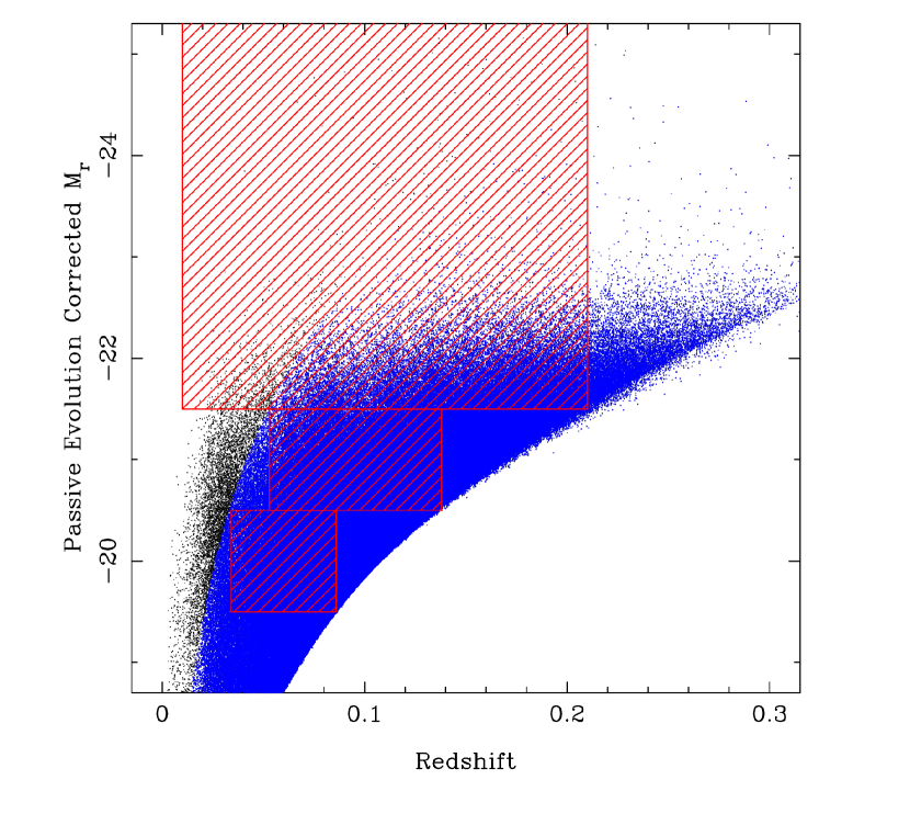
We construct the volume-limited samples by using corrected absolute $r$-band magnitude as a function of redshift. Our absolute $r$-band magnitudes use the NYU-VAGC convention: absolute magnitudes represent values at $z=0.1$ (see details in Blanton et al. 2005a). These are often written as $M_{{}^{0.1}\!{r}}$, which we simplify to $M_{r}$. Basically, passive evolution and $K$-corrections use the median redshift of the flux-limited SDSS Main sample to minimize uncertainties in their empirical determination. Formally, $M_{r}=M_{r}-5\log h$ but our unit convention sets $h=1$ making the last term unnecessary. We define a sub-sample of objects by selecting bounding redshifts which correspond to a specific luminosity range. We define three samples: a BRIGHT sample with $M_{r}<-21.5$, LSTAR with $-21.5<M_{r}<-20.5$, and FAINT with $-20.5<M_{r}<-19.5$. We show the selection of these samples in Figure 1. We tabulate their properties, such as the redshift range, volume, number of objects, and completeness corrected number density in Table 1.

Of particular concern might be the “fiber collision corrections” in the galaxy data. The correction used in the NYU-VAGC assigns the redshift of the nearest angular neighbor to a galaxy that does not have a redshift, reducing the number of collisions from $\sim 7\%$ to less than $\sim 4\%$. This correction was investigated using galaxy mocks in the 2PCF (Zehavi et al. 2002, 2005), and concluded that it works incredibly well for separations above the collision scale with only a small residual effect for redshift space quantities on all scales. We do not expect this correction to be appropriate for smaller scales. However, the fiber collision correction does not significantly affect our analysis as we focus on scales above $3\;h^{-1}\mathrm{Mpc}$. The collision scale at the largest redshift in our galaxy sample remains well below this value, as $55\arcsec$ corresponds to a separation of $\sim 0.13\;h^{-1}\mathrm{Mpc}$ at $z=0.21$.

Figure 1.— This figure depicts the selection of three volume-limited samples from the SDSS DR6 release detailed in Table 1 and shown as shaded boxes corresponding to BRIGHT, LSTAR, and FAINT (from top to bottom). Each point represents a galaxy, and the blue and black colors depict the two overlapping parent catalogs (a single galaxy can be in both catalogs). The black points correspond to NYU-VAGC bright which does not include a limit on a galaxy’s bright apparent magnitude. The blue points, overplotted on the black, correspond to NYU-VAGC safe and include a bright cut to the apparent magnitude (see Blanton et al. 2005a). We select redshift limits where galaxies of all included magnitudes can be seen at both the inner and outer boundaries.

Galaxy clustering measurements for SDSS have been shown to vary strongly with color (Zehavi et al. 2005, 2010). We investigate the color dependence on two of our samples (LSTAR and FAINT) by defining a simple red-blue split based on the $g-r$ color. There is a strong bi-modality between red and blue sub-samples that varies with absolute magnitude, as shown in Baldry et al. (2004). We adopt a simple linearly sloped color cut that depends on absolute $r$-band magnitude to account for the bi-modal distribution which separates the red sequence from the blue cloud, as described in Zehavi et al. (2005). Specifically, the $g-r$ color limit is

$$(g-r)_{lim}=0.21-0.03M_{r}\;.$$ (1)

Radial distances and absolute magnitudes are calculated using a flat $\Lambda\mathrm{CDM}$ cosmology with ($\Omega_{\mathrm{m}}=0.3\,,\,\Omega_{\Lambda}=0.7$).

2.2. Hubble Volume Simulation

We compare the SDSS galaxy distribution with the structure in cosmological $N$-body simulations. We use the Hubble Volume (HV) simulations (Colberg et al. 2000; Evrard et al. 2002) that were completed by the the Virgo Consortium. We choose the simulation with $\Lambda\mathrm{CDM}$ cosmology: ($\Omega_{\mathrm{m}}=0.3$, $\Omega_{\Lambda}=0.7$, $H_{o}=70{\,{\rm km}\,{\rm s}^{-1}\,{\rm Mpc}^{-1}}$, $\sigma_{8}=0.9$). This HV simulation consists of $1000^{3}$ particles in a box of $(3000\;h^{-1}\mathrm{Mpc})^{3}$ volume which evolves particles of mass $m_{\mathrm{part}}=2.2\times 10^{12}\;h^{-1}M_{\odot}$ from an initial redshift of $z_{init}=35$ to the current epoch using a Plummer softened gravitational potential where the softening length is $0.1\;h^{-1}\mathrm{Mpc}$. To better compare with observational galaxy samples, we utilize their “light-cone” realization. The light-cone output of the HV $\Lambda\mathrm{CDM}$ simulation was kindly provided by Gus Evrard and Jörg Colberg.

We treat the particles of the HV simulation like a potential observation and apply observational constraints to their distribution. We filter particles to match the same angular footprint of the SDSS geometry and radial distance to exactly reproduce the volume of the corresponding galaxy sample. We apply redshift distortions by using the peculiar velocity of the DM particle.

Finally, we randomly downsample the number of dark matter particles to make the computational time of the analysis more manageable. To verify this downsampling does not introduce a systematic bias, we perform a few measurements on several downsampled realizations and compare with the full DM distribution. We find minimal differences that are within expectations for Poisson sampling.

3. Theory & Methods

The $n$-point correlation functions provide a statistical description of LSS and remain a standard tool for quantifying the structure of the mass field and galaxy distribution (Peebles 1980). We summarize the basics relevant to this analysis below.

We can define density as a function of position, $\rho(\vec{x})$, that has an average density of $\bar{\rho}$. We define the fractional overdensity about the mean at a local point as

$$\delta(\vec{x})=\frac{\rho(\vec{x})}{\bar{\rho}}-1\;.$$ (2)

Casting the density in terms of the overdensity effectively removes the first moment of the $\delta$ field, i.e. $\langle\delta(\vec{x})\rangle=0$, where the $\langle\rangle$ denotes an ensemble average. The two-point correlation function (2PCF) can be defined in terms of $\delta$ values characterized by the separation of two positions, $r_{12}=|\vec{x}_{1}-\vec{x}_{2}|$, by assuming homogeneity and isotropy, and we write the 2PCF as

$$\xi(r_{12})=\langle\delta(\vec{x}_{1})\delta(\vec{x}_{2})\rangle\;.$$ (3)

A Gaussian field refers to any distribution that is fully described (statistically) by only its first and second moments (e.g. a mean and variance). For the $\delta$ field, the mean is zero and $\xi(r)$ successfully describes all clustering properties of a Gaussian field. Any other possible distribution is then non-Gaussian and can have non-trivial higher order moments (i.e. non-zero higher order correlation functions). Higher order functions can be similarly defined in terms of overdensity fluctuations, where the three-point correlation function (3PCF) is given by

$$\zeta(r_{12},r_{23},r_{31})=\langle\delta(\vec{x}_{1})\delta(\vec{x}_{2})\delta(\vec{x}_{3})\rangle\;.$$ (4)

Instead of a single dependent variable, such as $r_{12}$ in $\xi(r_{12})$, we see the 3PCF relies on three separations necessary to parameterize triplets. Further higher order correlation functions (greater than $n=3$) require even more variables and quickly result in a “combinatorial explosion” of parameters (Szapudi 2009).

The hierarchical ansatz posits that the 3PCF can be estimated by a cyclic combination of respective 2PCFs:

$$\zeta(r_{12},r_{23},r_{31})\approx Q\left[\xi_{12}\xi_{23}+\xi_{23}\xi_{31}+\xi_{31}\xi_{12}\right],$$ (5)

where we have simplified notation with $\xi_{12}=\xi(r_{12})$, and $Q$ denotes a scaling constant to adjust the amplitude. Initial measurements of 3PCF using angular surveys suggested that the hierarchical ansatz held at small scales with $Q\approx 1.3$ (Peebles 1980).

What was originally called the hierarchical amplitude ($Q$) can be rewritten as a function, specifically

$$Q(r_{12},r_{23},r_{31})=\frac{\zeta(r_{12},r_{23},r_{31})}{\xi_{12}\xi_{23}+\xi_{23}\xi_{31}+\xi_{31}\xi_{12}}\;.$$ (6)

This definition provides a useful normalization, and $Q(r_{12},r_{23},r_{31})$ is commonly referred to as the normalized or reduced 3PCF. As long as the the 2PCF remains well above zero, i.e. the denominator in (6), the value of the function $Q$ roughly equals unity regardless of scale. This functional form was later justified by gravitational perturbation theory, as the evolution of the 3PCF depends on quadratic terms in the equations of motion encapsulated in the square of the 2PCF (Bernardeau et al. 2002). An additional benefit of utilizing such a “ratio statistic”: we expect $Q$ to be insensitive to both time and cosmology. To leading order, $Q$ only depends on the spectral index and triangle configuration (see Figure 9 in Bernardeau et al. 2002).

3.1. Redshift Distortions and Projected Correlation Functions

Redshift distortions destroy the isotropy of the galaxy distribution. They arise from our inability to disentangle the peculiar (dynamical) velocity of a galaxy’s motion from the Hubble flow when determining the radial distance via the spectroscopic redshift. We characterize the correlation functions by a separation in real space (i.e. non-distorted), generally denoted as $r$. In practice, observations yield the distorted distance, and we refer to this redshift space separation as $s$. When the angle subtended by $s$ is small (i.e. the plane-parallel approximation), we can decompose the redshift space distance into a line-of-sight ($\pi$) and projected separation ($r_{p}$) such that $s=(\pi^{2}+r_{p}^{2})^{1/2}$. This effectively encapsulates the redshift distortion in the $\pi$ coordinate.

Redshift distortions (Jackson 1972; Sargent and Turner 1977; Peebles 1980) produce two clearly observable effects on the galaxy distribution (reviewed in Hamilton 1998). At small scales, gravitational collapse becomes highly non-linear and large peculiar velocities produce elongated structures in the radial direction affectionately referred to as fingers-of-god (the dominant effect at small $r_{p}$, see Jackson 1972). Larger scales exhibit a flattening from linear infall, observed as less obvious structures perpendicular to the line-of-sight (Kaiser 1987).

We can parameterize the redshift space 2PCF in terms of the plane-parallel approximation, $\xi(s)\rightarrow\xi(r_{p},\pi)$, and integrate along $\pi$ to produce the projected 2PCF:

$$w_{p}(r_{p})=2\int_{0}^{\pi_{\mathrm{max}}}\xi(r_{p},\pi)\mathrm{d}\pi\;.$$ (7)

Physically, we project the 3D correlation function onto a 2D surface of the sky in a moving annulus of fixed width according to $\pi_{\mathrm{max}}$. The projected 3PCF and its reduced form can be analogously defined as:

$$\zeta_{proj}(r_{p12},r_{p23},r_{p31})=\\ \iint\zeta(r_{p12},r_{p23},r_{p31},\pi_{12},\pi_{23})\mathrm{d}\pi_{12}\mathrm{d}\pi_{23}\;,$$ (8)

$$Q_{proj}(r_{p12},r_{p23},r_{p31})=\\ \frac{\zeta_{proj}(r_{p12},r_{p23},r_{p31})}{w_{p12}w_{p23}+w_{p23}w_{p31}+w_{p31}w_{p12}}\;.$$ (9)

We extended our simplified notation such that $r_{p12}$ is the projected analog to $r_{12}$, and $w_{p12}=w_{p}(r_{p12})$. We choose $\pi_{\mathrm{max}}=20\;h^{-1}\mathrm{Mpc}$ for the measurements we present in this work (discussed further in Appendix B).

Our notation is as follows. We show measurements of the 2PCF as a function of redshift space separation $s$. For projected space measurements, we keep the 2PCF characterized by a single dependent variable: $r_{p}$. The 3PCF is a function with three dependent variables and we continue the notation: $s$ or $r_{p}$ for redshift and projected space separations, respectively. Finally, our use of $r$ is more general and can refer to separation in (theoretical) real, redshift or projected space.

3.2. Estimating the Correlation Functions

We estimate the correlation functions using normalized pair counts for the 2PCF and triplets for the 3PCF. We use a class of unbiased and minimal variance estimators (see Szapudi and Szalay 1998) to optimally correct for edge effects. The estimator we use for the 2PCF was first presented by Landy and Szalay (1993):

$$\widehat{\xi}_{LS}=\frac{DD-2DR+RR}{RR}\;,$$ (10)

where $DD$ denotes the normalized data-data pairs, $RR$ represents the normalized random-random pairs and $DR$ corresponds to the normalized cross count of data-random pairs. The $LS$ estimator was extended for all $n$-point correlation functions by Szapudi and Szalay (1998), and we estimate the 3PCF as

$$\widehat{\zeta}_{SS}=\frac{DDD-3DDR+3DRR-RRR}{RRR}\;.$$ (11)

As before, $DDD$ represents the normalized count of data-data-data triplets, $DDR$ corresponds to data-data-random, etc.

We construct random catalogs that are a factor of $5-10$ greater in density than the data. We find this ratio sufficient to keep the shot noise contribution of the random catalogs well below that of the data for all triplet counts, as well as small enough to be computational manageable. We designed the random catalogs to have the exact redshift distribution as the data: for each galaxy, we generate $5-10$ points with random angular coordinates but identical redshifts. Finally, we match both the angular footprint and volume of the corresponding data samples.

For our pair and triplet counts, we employ an exact $n$-point calculator implemented in Ntropy, a parallel kd-tree framework (Gardner et al. 2007). The application, ntropy-npoint, utilizes an efficient algorithm developed by Moore et al. (2001) and discussed in Gray et al. (2004). Their original implementation, npt, is publicly available and has been used to investigate the 3PCF (Nichol et al. 2006; Kulkarni et al. 2007; Marín et al. 2008). The independent $n$-point implementation based on Ntropy shows enhanced runtime performance, true parallel capability, and the ability to search directly in projected coordinates of $r_{p},\pi$ (see details in Gardner et al. 2007). We define the coordinates $\pi$ and $r_{p}$ for each point pair, where the 3D separation is $\vec{r}_{12}=\vec{x}_{1}-\vec{x}_{2}$. We use the unit direction to the midpoint of the separation, $\widehat{r}_{m}$ to calculate $\pi=\widehat{r}_{m}\cdot\vec{r}_{12}$ and find $r_{p}^{2}=r^{2}_{12}-\pi^{2}$.

We stress that the ability to utilize massively parallel computing platforms proved extremely important, as the projected 3PCF required almost two orders of magnitude more time to compute than the spatial 3PCF. We utilized hundreds of processors at a time and required $\sim\!300,000$ CPU hours to complete the $n$-point calculations presented here.

3.3. Triplet Configurations and Binning Scheme

The full 3PCF is a function of three variables that characterize both the size and shape of triplets. A natural and unique description of a triplet is the length of each side of the triangle that connects the points: $r_{1}$, $r_{2}$ and $r_{3}$ where connectivity is assumed by $\vec{r}_{3}=\vec{r}_{1}+\vec{r}_{2}$.

In perturbation theory, it is most common to see triangles described by two side lengths ($r_{1}$ and $r_{2}$) and their opening angle ($\theta$) defined by the cosine rule:

$$\cos\theta=\frac{r_{1}^{2}+r_{2}^{2}-r_{3}^{2}}{2r_{1}r_{2}}\;.$$ (12)

We find this last characterization the most natural and intuitive and will use it to describe our 3PCF measurements. When $\theta\approx 0$ or $\theta\approx\pi$, we refer to triplets as “collapsed” or “elongated” respectively, both of which have two sides being very close to co-linear. As $\theta$ approaches $\pi/2$ the triplet forms a right triangle which we will refer to as a “perpendicular” configuration. The triangle shape, or configuration dependence, describes a function of $\theta$ where “strong configuration dependence” means a significant amplitude difference in the reduced 3PCF, $Q(r_{1},r_{2},\theta)$, between co-linear and perpendicular configurations and “weak configuration dependence” shows little or no change of in $Q(r_{1},r_{2},\theta)$ with $\theta$. This terminology relates to that used by Gaztañaga and Scoccimarro (2005).

While it might appear this description is both trivial and pedantic, we caution that these mappings are non-linear. Triangle descriptions such as side-side-side and side-side-angle remain completely equivalent for exact values when the triangle vertices are infinitesimal points. However, these transformations will not be exact for small volumes, as in the case of estimating correlation functions where we accumulate counts within bins of a finite width. Care must be taken to prevent significant discrepancies in 3PCF measurements if the parameterization used for the calculation differs from the one that is modeled. We carefully consider this subtlety to correctly interpret our measurements.

We choose ($r_{1}$, $r_{2}$, $\theta$) to parametrize our 3PCF measurements, although we measure the 3PCF using bins defined by ($r_{1},r_{2},r_{3}$) and use (12) to convert $r_{3}$ to $\theta$. Even though we treat the reduced 3PCF as a function of three variables, $Q(r_{1},r_{2},\theta)$, we may often denote it as $Q(\theta)$ of even $Q$ for simplicity.

A good choice of binning is not straightforward for the configuration dependence of the 3PCF. Since neighboring bins need to be tightly packed to measure $Q(\theta)$, choosing a bin-width based on $\log r$ will be too large and insufficient to resolve a slow variation. On the other hand, a small bin-size will quickly become under-sampled, as triplets are characterized by three variables. We choose to employ linearly spaced bins in $\theta$, and use the cosine rule in (12) to define the midpoint $r_{3}$. We choose a bin-width as a fraction, $f$, of the measured scale, $r$, such that $\Delta_{r}=f\times r$ and a bin at $r$ is measured between $(r-\frac{\Delta_{r}}{2},r+\frac{\Delta_{r}}{2})$. This scheme was independently found to be useful in a theoretical study of the 3PCF by Marín et al. (2008). We compare measurements between three volume-limited galaxy samples which have very different number densities (see Table 1), and select a single fraction $f$ to apply to all samples and scales for a fair comparison. We set the value of the fractional bin-width by requiring a “reasonable sampling” of the sparsest dataset: the BRIGHT galaxy sample. Using a fractional bin-width of 25% ($f=0.25$) results in several hundred triplet counts at the smallest scales ($r_{1}=3\;h^{-1}\mathrm{Mpc}$), and we use this $f$ value for all measurements. This produces relatively wide bins with some that physically overlap (the same triplet is counted more than once). We note two observable consequences: (1) a slight damping of the 3PCF near $\theta\approx\pi$, and (2) an induced correlation between some neighboring $\theta$ bins. Qualitatively, this should not pose a problem since all comparisons use the exact same scheme (including $N$-body results). Quantitatively, we account for this by using the full covariance matrix. We further discuss the implications of binning in the appendix, § A.3.

3.4. Estimating the Covariance Matrix

We measure the correlation between measurements by empirically calculating the covariance matrix. Given a number of realizations, $N$, a residual on $Q$ can be defined as

$$\Delta_{i}^{k}=\frac{Q_{i}^{k}-\bar{Q}_{i}}{\sigma_{i}}\;,$$ (13)

for each realization ($k$) and bin ($i$) given a mean value ($\bar{Q}_{i}$) and variance ($\sigma_{i}^{2}$) for each bin over all realizations. We use $Q$ as a general placeholder for any measured statistic (2PCF, 3PCF, etc). A covariance matrix can be estimated from the data itself using a leave one out cross validation method, more commonly referred to as jackknife re-sampling (see further description in Lupton et al. 2001).

The number of jackknife samples (which we denote with $N$) are not independent realizations, and the jackknife covariance matrix can be estimated by:

$$\mathcal{C}^{(jack)}_{ij}=\frac{(N-1)^{2}}{N}\mathcal{C}_{ij}=\frac{N-1}{N}\sum_{k=1}^{N}\Delta_{i}^{k}\Delta_{j}^{k}\;,$$ (14)

where $\mathcal{C}_{ij}$ denotes the typical unbiased estimator of the covariance when computed on jackknife samples. Jackknife re-sampling has been shown to be reliable on scales up to $30\;h^{-1}\mathrm{Mpc}$ for the 2PCF on spectroscopic galaxy samples when compared with independent mock catalogs (Zehavi et al. 2002, 2004, 2005). However, a more elaborate study by Norberg et al. (2009) highlights potential problems and caveats of using such an “internal” estimate of the errors. We defer questioning the validity of jackknife re-sampling methods for estimating the covariance of the reduced 3PCF to a companion paper (McBride et al. 2010). They compare jackknife estimates to those from mock galaxy catalogs generated from $N$-body simulations. They conclude that while jackknife error estimates do not exactly agree with mocks, they appear sufficient for the analysis presented here (McBride et al 2010).

We generate our jackknife samples using the pixelization scheme of STOMP . This code can account for the irregular geometry of the SDSS data, and has been used to quantify errors in angular clustering (Scranton et al. 2005). The jackknife regions are selected to maintain equal unmasked area on the sky. In the SDSS samples we use, survey depth does not vary over the sky, which makes equal area consistent with equal volume. We want to resolve the covariance of $Q(\theta)$ for $15$ bins in $\theta$ between $0$ and $\pi$, therefore using less than $15$ jackknife samples should formally result in a singular covariance matrix. We choose $30$ jackknife samples where the regions are each $\sim 180$ square degrees in unmasked area (see discussion in McBride et al. 2010 where they investigate varying the number of jackknife samples for these $Q(\theta)$ measurements).

4. SDSS Measurements

4.1. Two-Point Correlation Function

Figure 2.— The redshift space 2PCF, $\xi(s)$ in the left panel, and projected 2PCF, $w_{p}(r_{p})$ in the right panel, for our three SDSS samples. Brighter galaxy samples exhibit more clustering (e.g. higher amplitude) than fainter samples, in agreement with published analyses of SDSS galaxies (Zehavi et al. 2005). Error bars denote $1$$\sigma$ uncertainties calculated from 30 jackknife samples.

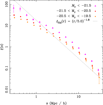
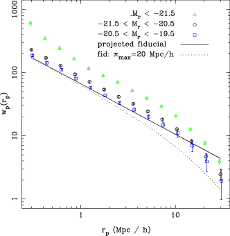
We first investigate the 2PCF of our samples. While we later focus our clustering analysis on the reduced 3PCF, $Q(r_{1},r_{2},\theta)$, it is instructive to directly examine the 2PCF since $Q$ is the ratio of the connected 3PCF, $\zeta(r_{1},r_{2},\theta)$ divided by products of the 2PCF, $\xi(r)$, such that $Q\propto\zeta/\xi^{2}$ as shown in (6). We choose equal width bins in $\log r$ to measure the 2PCF.

The galaxy correlation function was first shown to be a power law by Totsuji and Kihara (1969) using galaxy data from the Lick Observatory (Shane and Wirtanen, 1967). Along with our measurements, we plot a fiducial power law model,

$$\xi(r)=\left(\frac{r}{r_{o}}\right)^{-\gamma}\;;\;\xi_{fid}=\left(\frac{r}{5\;h^{-1}\mathrm{Mpc}}\right)^{-1.8},$$ (15)

which we adopt for comparison from a detailed study of clustering in SDSS galaxies by Zehavi et al. (2005). Given the precision of modern measurements, recent work has noted significant departures of the galaxy 2PCF from a power law (Zehavi et al. 2004) where the data are better described by the halo model (reviewed in Cooray and Sheth 2002). Nevertheless, a power law provides a simple and convenient comparison.

We plot the 2PCF in both redshift space, $\xi(s)$, and projected space, $w_{p}(r_{p})$, for our three galaxy samples in Figure 2. At larger scales, $\xi(s)$ runs almost parallel to the fiducial model for all galaxy samples. We note the reduction in strength of $\xi(s)$ at separations below $\approx 5\;h^{-1}\mathrm{Mpc}$ in Figure 2. At these scales this is an effect of redshift distortions where the fingers-of-god make galaxy pairs at close separations less likely and reduce the small scale correlation function.

In contrast to $\xi(s)$, the $w_{p}(r_{p})$ does not exhibit the same reduction in power, and remains close to a power law for small projected separations. This confirms our expectations that the projected $w_{p}(r_{p})$ should be less affected by redshift distortions – especially at the smaller projected scales (see Figure 2). At large $r_{p}$, $w_{p}(r_{p})$ shows a reduction of power due to truncating the $\pi$ integration at $\pi_{\mathrm{max}}=20\;h^{-1}\mathrm{Mpc}$. We show this effect by using our fiducial model. Assuming a perfect power law in real space, we depict the resulting $w_{p}(r_{p})$ with two lines in Figure 2, where the dotted line uses the same $\pi_{\mathrm{max}}$ as the data and solid line depicts the full projection (i.e. $\pi_{\mathrm{max}}=\infty$).

In both $\xi(s)$ and $w_{p}(r_{p})$ we note that brighter galaxies exhibit stronger clustering when compared to fainter galaxies. We can understand this in terms of a simple galaxy-mass bias parameter (Fry and Gaztanaga 1993), where $\xi\propto b^{2}$ and the linear bias, $b$, increases with galaxy luminosity; this has been studied in detail for SDSS galaxies(Zehavi et al. 2005, 2010). Our measurements are in agreement with their analysis. The galaxy 2PCF depicts a higher amplitude than the fiducial model, which is consistent with the luminosity of our galaxy samples.

4.2. Equilateral Three-Point Correlation Function

Figure 3.— The equilateral reduced 3PCF, $Q_{eq}(r)$, for our three SDSS galaxy samples, both in redshift space (left) and projected space (right). The equilateral reduced 3PCF is characterized by a single scale for simplicity: $Q_{eq}(r)=Q(r,r,r)$. We choose a bin-size to be equal width in $\log r$ analogous to the binning we used for the 2PCF. Error bars denote $1$$\sigma$ uncertainties calculated from 30 jackknife samples.

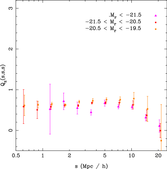
The simplest analog to the 2PCF is the equilateral reduced 3PCF, $Q_{eq}(r)$. As each side of the triangle formed by a triplet corresponds to the same scale ($r_{1}=r_{2}=r_{3}=r$), $Q_{eq}$ can easily be characterized by a single separation:

$$Q_{eq}(r)=\frac{\zeta(r,r,r)}{3\;\xi(r)^{2}}\;.$$ (16)

$Q_{eq}$ is not sensitive to shape, but it provides a clear sense of scale dependence in the reduced 3PCF. When $Q_{eq}\!\approx 1$, the number of triplets exactly correspond to those expected from the 2PCF; when $Q_{eq}$ is above or below $1$, there are more or less triplets, respectively. Like the 2PCF, we choose bins of equal width in $\log r$.

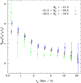
We show $Q_{eq}$ in both redshift and projected space for our three galaxy samples in Figure 3. In redshift space, $Q_{eq}$ appears flat and never exceeds $1$, showing very little difference in terms of luminosity. In the projected measurement, small scales reveal $Q_{eq}>1$ until $r_{p}\approx 2-3\;h^{-1}\mathrm{Mpc}$, where it approximately reproduces the amplitude of the redshift space measurement. We expect larger scales to dip below one, as $\zeta(r)$ drops more rapidly than pairs in the 2PCF for the same scale. Intuitively, the number of equilateral triplets of a set side length become more rare than the number of available pairs of the same separation length.

On small scales redshift distortions destroy small scale triplets in a manner similar to what we discussed for pairs in the 2PCF. We notice that redshift space $Q_{eq}$ remains flat in Figure 3, but the projected $Q_{eq}$ recovers power at small $r_{p}$. This suggests the flattening of the redshift space measurement is a result of redshift distortions. This interpretation is supported by a theoretical comparison of the real and redshift space $Q_{eq}$ in Marín et al. (2008) (see their Figure 1). We notice a slight variation of the measurement with sample luminosity, but not nearly as pronounced as seen in the 2PCF, and only significant for a few points. At the largest scales ($r\geq 10\;h^{-1}\mathrm{Mpc}$), the reduction in amplitude of $Q_{eq}$ and increased size of the errors suggest that we are limited in signal by the finite volume of the galaxy sample. The effects appear worst for the faintest volume-limited sample, which is expected since it also occupies the smallest volume in comparison with the larger volume brighter samples (see Table 1). Finite volume effects have been shown to cause a rapid reduction in amplitude for higher order measurements of clustering (Scoccimarro 2000).

4.3. Configuration Dependence of reduced 3PCF

We focus our investigation on the shape or configuration dependence of the reduced 3PCF, $Q(r_{1},r_{2},\theta)$. The reduced 3PCF was analyzed in redshift space by Kayo et al. (2004) and Nichol et al. (2006) using a previous release of SDSS galaxy data: “sample12” – a version between the first and second data releases covering $\sim\!2406$ square degrees. Unlike these previous studies, we restrict our analysis only to volume-limited galaxy samples, and jointly investigate redshift and projected space measurements. We measure the reduced 3PCF for SDSS DR6 galaxies at three scales, which we specify by the smallest side of the triangle, $r_{1}$. We choose $r_{2}$ so that the ratio of the first two sides stays fixed such that $r_{2}/r_{1}=2$. We then measure the reduced 3PCF as a function of opening angle between these two sides, $\theta$, regularly spaced between $0$ and $\pi$. The resulting scale we probe varies from $r_{1}$, when $\theta=0$ (i.e. “collapsed”) to $(r_{1}+r_{2})$, when $\theta=\pi$ (i.e. “elongated”). Specifically we measure triplets on scales between $3-9$, $6-18$ and $9-27\;h^{-1}\mathrm{Mpc}$ corresponding respectively to $r_{1}=3,6$ and $9\;h^{-1}\mathrm{Mpc}$.

Figure 4.— The reduced 3PCF on SDSS DR6 galaxies showing both redshift space and projected measurements. The filled symbols are redshift measurements, and the hollow symbols are projected. Triangles correspond to $M_{r}<-21.5$, circles with $-21.5<M_{r}<-20.5$ and squares with $-20.5<M_{r}<-19.5$. The three columns are different scales, specified by the first side of the triangle ($r_{1}$) representing the smallest scale measured. Error bars denote $1$$\sigma$ uncertainties calculated from 30 jackknife samples.

We introduce the configuration dependence for each sample and scale in Figure 4, where we overlay the reduced 3PCF in both redshift and projected space. On smaller scales (left side of Figure 4), we see weaker configuration dependence in the reduced 3PCF (i.e. smaller change in $Q(\theta)$ with $\theta$) than at the larger scales (right side).

We notice a “V-shape” at $r_{1}=9\;\;h^{-1}\mathrm{Mpc}$, present in both redshift and projected space measurements of Figure 4. We interpret this as a statistical signal of filamentary structure that becomes more pronounced as the scale increases: an over-abundance ($Q>1$) of co-linear triangles with an under-abundance ($Q<1$) of perpendicular configurations. This characteristic V-shape is predicted from gravitational perturbation theory (Bernardeau et al. 2002) as well as results from simulations (Gaztañaga and Scoccimarro 2005; Marín et al. 2008).

We identify the effect of redshift distortions on the small scales in the redshift space reduced 3PCF in two ways: (1) almost no configuration dependence in $Q_{z}(\theta)$ and (2) $Q_{z}(\theta)<1$ for all configurations, showing a deficiency of triplets due to non-linear velocities stretching compact structures beyond the scales probed (i.e. fingers-of-god). On small scales, we notice that $Q_{proj}$ has both a higher amplitude and exhibits a stronger configuration dependence in comparison with $Q_{z}$. When comparing with the 2PCF (Figure 2), the projected measurements are larger in amplitude. However, $Q_{proj}$ is normalized by $w_{p}(r_{p})$, so we expect $Q_{proj}$ to match $Q_{z}$ and remain close to $1$ in value. The increased amplitude of $Q_{proj}$ is attributed to recovering signal that was lost to $Q_{z}$ due to redshift distortions. We consider the stronger configuration dependence of $Q_{proj}$ reflective of the true galaxy distribution, as a simple projection should not increase the configuration dependence. We conclude that the projected measurement recovers signal that is destroyed in the redshift space measurement due to non-linear distortions. However, we expect that our choice of $\pi_{max}=20\;h^{-1}\mathrm{Mpc}$ will permit redshift distortions to affect these projected measurements, albeit in a reduced capacity with respect to redshift measurements. As the scale increases beyond $9\;h^{-1}\mathrm{Mpc}$, $Q_{proj}$ and $Q_{z}$ generally converge (right column of Figure 4).

We see a dramatic difference in the size of uncertainties between these measurements. For each individual sample and statistic, there are two important aspects to consider. First, the small scales become sensitive to sampling where a galaxy sample with a lower number density will be less well determined (shot noise limited). Second, the larger scale measurements will show more sensitivity to volume effects (being dominated by sample or cosmic variance). We see this same behavior for $Q_{eq}$ in Figure 3.

The uncertainties increase with larger scales, especially for the fainter galaxy samples. We actually expect the growth of errors from the “ratio” static of the reduced 3PCF since we predict the reduced 3PCF to be approximately unity at all scales. We interpret the general increase of errors on $Q$ as the higher order 3PCF (numerator in $Q$) becoming uncertain at a much faster rate than the 2PCF (denominator).

We notice the uncertainties on the FAINT sample appear much larger than measurements on the two brighter samples, especially at larger scales. This is not Poisson uncertainty as the sample contains over 76,000 galaxies, a factor of two greater than the BRIGHT sample. The FAINT galaxy sample occupies a much smaller volume, and a few large structures dominate the errors in the large scale measurements (see discussion in §4.5). The observed increase of uncertainties with fainter galaxy samples is generally a consequence of the smaller volume being probed by the fainter volume-limited samples (see Table 1).

The projected $Q(\theta)$ shows larger uncertainties than redshift space measurements at all scales. This is a natural side effect of the projection: a given scale in $r_{p}$ represents a lower bound on the redshift space scale, $s$, where the upper bound is $s=(\pi_{\mathrm{max}}^{2}+r_{p}^{2})^{1/2}$. Since $Q(\theta)$ at any given value of $r_{p}$ is sensitive to scales greater than the same value of $s$, it will encode properties of the larger scales. As the uncertainty grows with scale, $Q_{proj}$ will reflect higher uncertainties than $Q_{z}$ when $r_{p}\approx s$.

4.3.1 Luminosity Dependence

Figure 5.— The reduced 3PCF on SDSS DR6 galaxies, comparing the three samples of different magnitude limits. Triangles correspond to $M_{r}<-21.5$, circles with $-21.5<M_{r}<-20.5$, and squares with $-20.5<M_{r}<-19.5$. The top row contains redshift space measurements, and the bottom row depicts the projected measurements. The three columns are different scales, specified by the first side of the triangle ($r_{1}$) representing the smallest scale measured. Error bars denote $1$$\sigma$ uncertainties calculated from 30 jackknife samples.

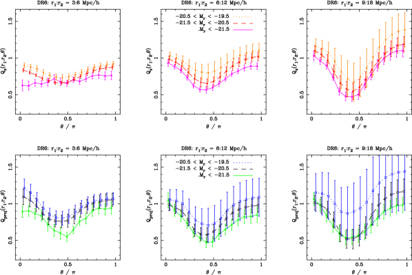
To highlight the effect of luminosity on the reduced 3PCF, we present the measurements of all three samples in Figure 5. As we noted in the 2PCF, the luminosity of the sample affects the clustering strength. However, we see the opposite behavior in $Q(\theta)$ as brighter galaxies show lower values of $Q$ than fainter galaxies. Also remember that in the 2PCF (Figure 2) brighter galaxies showed a stronger segregation with galaxy luminosity. If brighter galaxies exhibit stronger clustering, they will have a correspondingly higher linear bias $b$. Since $\xi\propto b^{2}$, the amplitude will be more sensitive to changes in $b$ as opposed to the reduced 3PCF, where $Q\propto 1/b$. The difference of $Q(\theta)$ with sample luminosity appears constant, or slightly increases, with scale.

Physically, we expect bright galaxies to predominantly live in galaxy groups or clusters and centered at the “knots” in LSS. Fainter galaxies will be more populous in the field and overdense filaments, which might show more configuration dependence in the reduced 3PCF. The uncertainties on these measurements prevent a clear demonstration of this effect – though we might speculate that a few measurements at $r_{1}=9\;h^{-1}\mathrm{Mpc}$ hint at fainter samples showing a stronger configuration dependence (e.g. LSTAR vs BRIGHT in lower right panel of Figure 5)

4.3.2 Color Dependence

We investigate the color dependence of the reduced 3PCF using two volume-limited samples, designed to have unit magnitude bins with limiting $r$-band magnitudes below and above $L_{\ast}$. We divided the galaxies into “red” and “blue” sub-samples to probe the color dependence as described in §2.

Figure 6.— We show the configuration dependence of the reduced 3PCF for our FAINT galaxy sample with $-20.5<M_{r}<-19.5$. The sample is divided into “red” (red, dashed line) and “blue” (blue, dotted line) sub-samples based on SDSS $g-r$ color (see sample description for details). The top row consists of redshift space measurements, and the bottom row depicts projected measurements. The three columns correspond to different scales specified by the first side of the triangle ($r_{1}$) representing the smallest scale measured. The black line denotes measurements on dark matter in the Hubble Volume simulation, but matching the selection of the galaxies and includes redshift distortions. Error bars denote $1$$\sigma$ uncertainties calculated from $30$ jackknife samples.

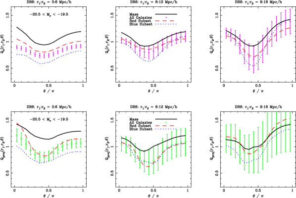
We examine the reduced 3PCF of the FAINT sample ($-20.5<M_{r}<-19.5$) in Figure 6. We see configuration dependence at all scales, and the V-shape becomes more prevalent on larger scales; behavior that is reflected in both color sub-samples. The red and blue galaxies show a larger disparity at smaller scales, with a significant increase in the clustering difference at $r_{1}=3\;h^{-1}\mathrm{Mpc}$ for both the redshift space and projected $Q(\theta)$. Unlike the luminosity dependence, we notice a significant change in the configuration dependence between the color samples. This effect is most noticeable in the $r_{1}=3\;h^{-1}\mathrm{Mpc}$ configuration for the projected $Q(\theta)$, which shows the red galaxies with a stronger configuration dependence than either the blue or full samples. At configurations where $r_{1}\geq 6\;h^{-1}\mathrm{Mpc}$, the blue sub-sample shows greater configuration dependence than the red, which can be best seen in redshift space. Overall, red galaxies typically show larger values of $Q(\theta)$ than the blue and full samples.

Figure 7.— We show the configuration dependence of the reduced 3PCF, as in Figure 6, but for the brighter LSTAR galaxy sample defined by $-21.5<M_{r}<-20.5$. The sample is divided into “red” (red, dashed line) and “blue” (blue, dotted line) sub-samples based on SDSS $g-r$ color (see sample description for details). The top row consists of redshift space measurements, and the bottom row depicts projected measurements. The three columns correspond to different scales specified by the first side of the triangle ($r_{1}$) representing the smallest scale measured. The black line denotes measurements on dark matter particles from the Hubble Volume simulation, but matching the selection of the galaxies and includes redshift distortions. Error bars denote $1$$\sigma$ uncertainties calculated from $30$ jackknife samples.

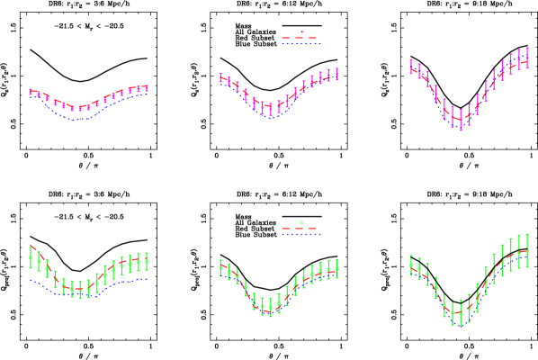
We show the reduced 3PCF for our LSTAR sample ($-21.5<M_{r}<-20.5$) in Figure 7. We still see configuration dependence at all scales, including color sub-samples — but the color dependence appears diminished with respect to the FAINT sample in Figure 6. Again, the red galaxies at $r_{1}=3\;h^{-1}\mathrm{Mpc}$ show a stronger configuration dependence than the blue according to $Q_{proj}$. This sample has a volume almost four times larger than the FAINT sample, and the large scale $r_{1}=9\;h^{-1}\mathrm{Mpc}$ measurements show significantly smaller uncertainties. As we speculated before, the blue galaxies appear to have a slightly stronger configuration dependence.

Although the difference between red and blue sub-samples is both small and within the reported uncertainties, it might be significant as the errors are dominated by cosmic variance. If the blue sub-sample does have a stronger configuration dependence than the red sub-sample, it would support the typically understood notion that blue galaxies more commonly populate the filamentary structures at these scales.

On smaller scales ($r_{1}=3\;h^{-1}\mathrm{Mpc}$), the blue sub-sample in projected space shows less configuration dependence than the red in both samples. We attribute this to a real clustering difference that is obscured by redshift distortions in the redshift space measurements. However, both $Q_{z}$ and $Q_{proj}$ show differences in the amplitude between “red” and “blue” populations at the smaller triangle scales, but this difference declines at the larger scales.

4.3.3 Comparing Galaxy and Mass Clustering

In Figures 6 and 7, we also plot measurements of the reduced 3PCF based on the dark matter particles in the Hubble Volume (HV) simulation. Using $N$-body simulations enables reliable predictions well into the non-linear regime where accurate analytic models do not exist (although some recent work has been introduced, see Smith et al. 2008). In addition, we can include observational systematics by trimming HV particles to match the exact selection and volume of the observed galaxy sample, and include the effects of redshift distortions. The HV measurement serves as a comparison between clustering of the observed galaxies and that expected from gravitational evolution of a $\Lambda\mathrm{CDM}$ mass field. Examining the figures, we make two observations: (1) the general shape is similar to that of the galaxy reduced 3PCF, and (2) there is a significant offset in amplitude between galaxies and mass.

Figure 8.— We show the configuration dependence of the reduced 3PCF of SDSS DR6 galaxies with $M_{r}<-21.5$. The top row consists of redshift space measurements, and the bottom row depicts projected measurements. The three columns correspond to different scales specified by the first side of the triangle ($r_{1}$) which represents the smallest scale measured. The black line denotes measurements on dark matter in the Hubble Volume simulation, matching the selection of the galaxies and includes redshift distortions. Error bars denote $1$$\sigma$ uncertainties calculated from $30$ jackknife samples.

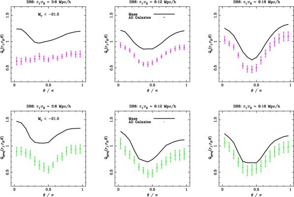
We show our measurement of the reduced 3PCF $Q$ on our BRIGHT galaxy sample ($M_{r}<-21.5$) in Figure 8. As shown previously, the black line depicts measurements from the HV simulation in comparison to the symbols that denote the galaxy measurements. The BRIGHT galaxy sample covers the largest volume, but is a factor of 10 less dense than the LSTAR sample and almost $30$ times less dense than FAINT.

It remains clear that galaxies do not cluster exactly the same as the simulated mass field. However, there are significant commonalities. The overall shape is the same, and the predominant effect is an offset. Remember, the nature of the reduced 3PCF makes it insensitive to cosmology (excepting the slope of the power spectrum), so the differences we observe in $Q$ are unlikely to be due to variation in assumed cosmology by the HV simulation. There is a large volume of work showing that galaxies are known to be biased tracers of the mass field, which offers a natural explanation of the offset (Cooray and Sheth 2002). The luminosity dependence of the reduced 3PCF discussed in §4.3.1 is further evidence of the same. The difference between clustering of galaxies and the underlying mass distribution is commonly referred to as galaxy-mass bias and depends on galaxy properties such as luminosity. We constrain the non-linear galaxy-mass bias parameters relating to these measurements in a companion paper (McBride et al. 2010).

4.4. Covariance of Galaxy Samples

Correctly accounting for the covariance in data measurements is essential to accurately constrain theoretical models. If significant covariance exists, neglecting it can result in a statistical bias (inaccurate constraints) or an overestimate of significance. However, proper estimation and use of the covariance matrix remains tricky. For statistical measures of clustering in LSS, the covariance matrix encodes higher-order information. The covariance matrix of the 2PCF includes significant third and fourth order terms, whereas the covariance of the 3PCF has leading order contributions from up to sixth order. The covariance matrix itself is a complementary measure of clustering.

We typically use the inverse of the covariance matrix to constrain models, such as a common $\chi^{2}$ determination. Doing this makes an analysis extremely sensitive to the noise properties of the covariance matrix (the poorest determined eigenmodes can have a dramatic impact on the $\chi^{2}$ value). While this fact is often overlooked in LSS analyses, ways of accounting for poorly resolved modes are well established for the 2PCF (see e.g. Norberg et al. 2009) and 3PCF (see e.g. Gaztañaga and Scoccimarro 2005). If a measured statistic is poorly resolved, i.e. the dominant contribution to the error is shot-noise, the off-diagonal elements of the covariance matrix can become excessively noisy. In such a case, using the full covariance matrix might be a poorer choice than a diagonal approximation (demonstrated in Chen and Szapudi 2006).

For our galaxy samples, we resolve the covariance matrix using jackknife re-sampling methods defined by $30$ equal-area regions on the sky (a factor of two over the number of measured bins).

Figure 9.— The normalized covariance matrix for the 2PCF, both in redshift (top row) and projected space (bottom row) for our three DR6 galaxy samples of different magnitudes. From left to right, the panels indicate FAINT to BRIGHT galaxy samples. The matrix is normalized such that diagonal elements are set to unity, rather than the $1$$\sigma$ error. The solid, dashed and dotted contours correspond respectively to values of 0.70, 0.85 and 0.99.

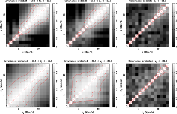
We show the normalized covariance matrix of the 2PCF for our three galaxy samples in Figure 9. At these scales we expect significant correlation in the covariance matrix for all the 2PCF measurements. In the power spectrum we expect the Fourier modes to be statistically independent (Bardeen et al. 1986) and the off-diagonal elements of the covariance matrix in the 2PCF preserve this Fourier space property. We note the BRIGHT sample (right column) appears almost diagonal. Since we still expect correlated bins for the sample, we interpret this result as an undersampled covariance matrix. This can occur when the most significant contribution is shot-noise (since Poisson errors are not correlated). While this is still a “true” measure of the errors, care must be taken when using the full covariance matrix as the off-diagonal elements can be noisy. For the two fainter samples, we see the projected $w_{p}(r_{p})$ measurements appear much more correlated than the redshift space $\xi(s)$. Since $w_{p}$ projects along the line-of-sight, the projection mixes scales between ($s=r_{p}$) and ($s=(\pi^{2}+r_{p}^{2})^{1/2}$), inducing a correlation in the measurements. Seeing this effect supports the validity our of covariance estimation. Finally, we note that the correlation appears to increase for the fainter galaxy sample. In the 2PCF, this increase of correlation with fainter galaxy samples has been previously seen (Zehavi et al. 2005).

Figure 10.— The normalized covariance matrix for the reduced 3PCF, both in redshift (top row) and projected space (bottom row) for our three DR6 galaxy samples of different magnitudes. From left to right, the panels indicate FAINT to BRIGHT galaxy samples. The matrix is normalized such that diagonal elements are set to unity, rather than the $1$$sigma$ error. This shows only the covariance for the largest triangles where $r_{1}=9\;h^{-1}\mathrm{Mpc}$. The solid, dashed and dotted contours correspond respectively to values of 0.70, 0.85 and 0.99.

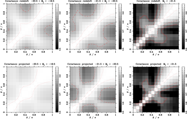
The covariance matrices for the reduced 3PCF on large scales ($r_{1}=9\;h^{-1}\mathrm{Mpc}$) for the three galaxy samples are shown in Figure 10. Note the significant off-diagonal structure for all samples, which is comparable to that seen in theoretical studies (see figure 9 in Gaztañaga and Scoccimarro 2005). The correlation between a few neighboring bins at $\theta\approx\pi$ is enhanced due to physical overlap of our binning scheme (the same triplet can be counted more than once). We again see that the correlation in the projected measurements indicate more correlation in comparison to redshift space. Analogous to the 2PCF, we find that fainter galaxy samples appear to have increased correlation between bins of the reduced 3PCF. Although we show only the largest measurements, we find significant off-diagonal elements at all scales. Clearly the use of a diagonal approximation to the covariance matrix would be a poor assumption.

4.5. Effects of Super Structures

Large coherent structures or “super structures”, such as the Sloan Great Wall (SGW; Gott et al. 2005), can dramatically affect clustering measurements. Detailed analyses on SDSS galaxy samples have documented this in both the 2PCF (Zehavi et al. 2002, 2005, 2010) and redshift space reduced 3PCF (Nichol et al. 2006). One advantage of using jackknife re-sampling methods for error analysis is that we probe the variation between different spatial regions essentially “for free”. We investigate this variation using our $30$ jackknife samples. There are several reasons this variation of the 3PCF is worth investigation beyond that in the literature. First, our samples are based on a newer SDSS sample (DR6) which includes additional regions of the sky resulting in a larger volume than previous studies. Second, as we have repeatedly mentioned, measurements of the reduced 3PCF are affected by a chosen binning scheme making it important to document the effects of structures given our exact parameterization. Finally, we want to understand the impact on detailed measurements of the projected reduced 3PCF for which the effect of super structures has not been previously investigated.

We identify $6$ out of $30$ regions of the sky which show large deviations in the reduced 3PCF. These “jackknife regions” characterize a jackknife sample by being omitted from a clustering measurement. The northern SDSS DR6 footprint in shown in Figure 11, with the entire sample displayed in gray and the six regions highlighted by color. Two regions encapsulate the majority of the SGW, specifically the red and magenta regions at a J2000 declination of zero. Overall, the jackknife regions appear contiguous and rectangular (excepting the apparent geometry of the Aitoff sky projection). Please note the black region, however, which is split between two sides of the survey. The algorithm we use to define the jackknife regions must occasionally make such divisions.

Before examining the reduced 3PCF for these regions, let us briefly review the jackknife re-sampling method. We excise a jackknife region from the full sample and measure the clustering. This means that a measurement on a specific jackknife sample represents the clustering of the entire sample omitting the jackknife region. If the clustering on the jackknife sample deviates strongly from the average of all samples, it means that a specific jackknife region dominates the measurement for the entire sample. Without that region, the overall clustering would be significantly different. This is a profound concept, as we do not expect such clustering differences given the volume of these SDSS samples.

We investigate the effects on the reduced 3PCF in two of our three galaxy samples. Although the jackknife regions based on sky location are consistent across both, the redshift limits vary. This results in a volume that is not identical between samples, although it does overlap. We use our LSTAR ($-21.5<M_{r}<-20.5$) and FAINT ($-20.5<M_{r}<-19.5$) samples which both include the SGW at a mean redshift at $z\approx 0.08$.

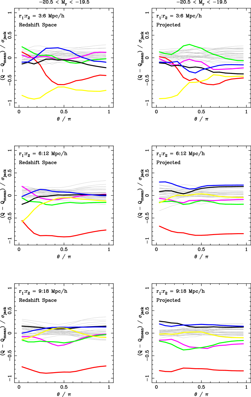
To highlight the clustering deviations between samples, we plot the residual of the reduced 3PCF, as defined by (13). We subtract the mean reduced 3PCF of the $30$ samples from each individual measurement, and normalize this difference by the jackknife variance. As noted in (14), the prefactor for the jackknife variance is ($\frac{N-1}{N}$), and not the familiar $\frac{1}{N}$, so error estimates do not decrease with $N$. In terms of the residuals, this means no jackknife sample will deviate significantly beyond the error. This scaling of the residuals emphasizes how each jackknife region significantly contributes to the $1\sigma$ error estimate.

Figure 11.— We show six selected jackknife regions on the sky (yellow, blue, black, green, magenta, and red) in comparison with the full galaxy sample (grey points) for the SDSS DR6 North footprint in J2000 equatorial coordinates. The Sloan Great Wall (Gott et al. 2005) is located at $\sim 0$ in declination, and is included in two of the six selected jackknife regions (red and magenta).

Figure 12.— The residuals, as defined in (13), for 30 jackknife samples of the reduced 3PCF in redshift and projected space for the DR6 galaxies with $-21.5<M_{r}<-20.5$. A jackknife sample is defined by taking the full sample and excluding a specific jackknife region. Colors of the six selected jackknife samples correspond to excluding galaxies in the region of matching color in Figure 11.

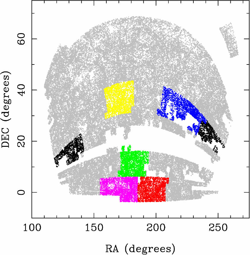
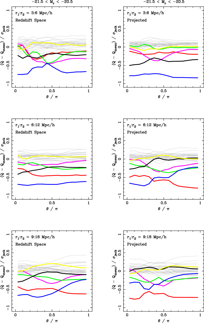
Figure 12 shows the residual of the reduced 3PCF for the LSTAR galaxy sample ($-21.5<M_{r}<-20.5$). The left three panels are results for redshift space, $Q_{z}$, and the right correspond to projected space, $Q_{proj}$. The scale increases downward in order with $r_{1}=3,6$ and $9\;h^{-1}\mathrm{Mpc}$. The gray lines represent results from the $30-6=24$ “ordinary” jackknife samples. The colored lines correspond to jackknife samples that omit the jackknife regions highlighted in Figure 11. Most of the regions are close to the mean value (i.e. around zero), but several samples deviate, which always happens in the negative direction. If a structure in the jackknife region, which is included in all other samples, boosts $Q(\theta)$, then a negative residual results. In the LSTAR sample, $Q_{z}$ appears to be boosted at all scales by galaxies in the blue jackknife region. As scale increases, structure in the red region also appears to increase $Q_{z}$. Both regions also have an effect on $Q_{proj}$, with red clearly dominating at $r_{1}=9\;h^{-1}\mathrm{Mpc}$ and blue at the small scale $r_{1}=3\;h^{-1}\mathrm{Mpc}$ measurement. In $Q_{proj}$, we note the black region, which is a physical neighbor to the blue region, strongly affects the small scale reduced 3PCF.

It appears the red region, which encloses a significant portion of the SGW, predominantly affects the reduced 3PCF on large scales; this has been seen before in the reduced 3PCF by Nichol et al. (2006). The blue and neighboring black regions were first included in the DR5 release. At smaller scales, these regions clearly dominate the reduced 3PCF measurement. We visually inspect the galaxy distribution within the several of the anomalous regions, and find that these jackknife regions (consisting of $1/30$ of the entire SDSS area) enclose a single dominant super structure, or sometimes just part of one structure straddled across several regions. For example, there is an extremely clustered region at the boundary of the blue and black regions with a median redshift around $z\approx 0.11$. This is clearly distinct from the SGW. We refer to such regions as “super” structures since, like the SGW, they are coherent overdensities that are not gravitationally self-bound in contrast to a galaxy cluster. Individually, these regions shift the reduced 3PCF by less than 10% – but this analysis neglects cumulative effects (remember, the same super structure is split between the blue and black regions).

We examine the FAINT galaxy sample ($-20.5<M_{r}<-19.5$) in Figure 13. Recall from the reduced 3PCF measurement in Figure 6, that the uncertainties were quite large, much more than the LSTAR sample. The residuals at the large scales are completely swamped from the clustering in the red region. Excluding this region changes the reduced 3PCF by approximately $20\%$, which we attribute to galaxies clustered in the SGW. The black and blue regions seem inconsequential for this sample; this makes sense as this fainter sample has a maximum redshift of $z=0.086$, thereby trimming the structure at $z\approx 0.11$ which accounted for the significant deviation in the LSTAR sample. We also see that a new region, denoted in yellow, dominates at small scales.

Figure 13.— The analogous figure to 12: the residuals as per (13), for 30 jackknife samples of the reduced 3PCF in redshift and projected space for the DR6 galaxies with $-20.5<M_{r}<-19.5$. A jackknife sample is defined by taking the full sample and excluding a specific jackknife region. Colors of the six selected jackknife samples correspond to excluding galaxies in the region of matching color in Figure 11.

5. Discussion

Our clustering measurements on our galaxy samples produced the following main results:

• $Q(\theta)$ exhibits configuration dependence at all scales ($3-27\;h^{-1}\mathrm{Mpc}$), which is not consistent with $Q$ being simply a constant.

• Larger scales ($9-27\;\;h^{-1}\mathrm{Mpc}$) exhibit a stronger configuration dependence and display the V-shape expected from gravitational evolution.

• All galaxy samples show significantly different clustering strength than the mass estimates.

• Uncertainties for the reduced 3PCF increase for larger scales and with smaller sample volume.

Generally, the shape of our SDSS galaxy measurements appear similar to predictions of gravitational collapse in the $\Lambda\mathrm{CDM}$ model realized by the Hubble Volume simulation. The difference in clustering strength between galaxies and mass predictions can be accounted for as galaxies of these luminosities are expected to be biased tracers of the mass field. We constrain the non-linear galaxy-mass bias using a detailed error analysis in a companion paper (McBride et al. 2010).

We studied measurements of three galaxy samples characterized by different luminosities, attributing observed variations as a luminosity dependence in the reduced 3PCF. In §4.3.1 we found:

• Luminosity dependence affects all scales at about the same level, which primarily changes the amplitude of $Q$.

• The discrepancy between galaxies and mass predictions appears larger for brighter galaxies.

• The covariance matrix appears more correlated for fainter galaxy samples.

The division of two volume-limited samples into sub-populations based on color led to these observations:

• The $g-r$ color split isolates populations with different clustering properties,

• Red sub-samples have a higher average $Q$ value than blue.

• The difference between red and blue sub-samples is greatest at small scales and includes changes to the configuration dependence.

• The effects of galaxy color on $Q$ are more pronounced than luminosity at small scales, where galaxy color more dramatically affects the configuration dependence.

A concern might arise that the defined samples are not complete for both color definitions. This could result from possible evolutionary effects (discussed in the context of DEEP2 in Gerke et al. 2007) or inaccuracies in the $K$-correction due to differences in galaxy morphology. We confirmed that there were minimal to no differences in the measured reduced 3PCF by creating samples defined to be more conservative in their sample description, where we found the largest variation to be less than 10% of the reported errors.

An analysis of the 2PCF for SDSS galaxies (Zehavi et al. 2005, 2010) conceptually explains the clustering difference of the brighter galaxy samples. Brighter galaxies remain “more biased” than fainter samples resulting in a larger discrepancy between galaxies and mass for brighter galaxy samples. We see a similar result in our clustering measurements and find that $Q$ shows less discrepancy between samples since $Q\propto 1/b$ whereas $\xi\propto b^{2}$ (“more biased” refers to a higher linear bias value of $b$). The stronger effect of color separation on smaller scales ($3-9\;h^{-1}\mathrm{Mpc}$) agrees with the conclusions of Blanton et al. (2005b) that galaxy color is strongly tied to local environment. Recent analysis of the 2PCF by Zehavi et al. (2010) showed striking differences in clustering between luminosity and color, where luminosity predominately shifts the amplitude, whereas different color samples show a different slope of the 2PCF. We find that the configuration dependence of $Q_{proj}$ is stronger for red sub-samples at smaller scales ($r_{1}=3\;h^{-1}\mathrm{Mpc}$). This scale is still beyond a reasonable size for individual dark matter halos. However, it might suggest that regions outside large halos have a surrounding anisotropic distribution of red galaxies, perhaps tracing the infall regions. This interpretation supports observations of the angular distribution of satellite galaxies by Azzaro et al. (2007), where they find an alignment of satellites along the major axis of their host. They find the strongest evidence of alignment when considering red satellites of red hosts, which would be best represented by our red sub-sample. On measurements of large scale triangles ($r_{1}=9\;h^{-1}\mathrm{Mpc}$), we conclude that both red and blue populations exhibit similar configuration dependence given the large errors. However, we speculate that the blue galaxies occupy regions that show stronger shape dependence.

A detailed study of the reduced 3PCF in redshift space (Gaztañaga et al. 2005) was conducted on a different redshift survey: the two-degree field galaxy redshift survey (2dFGRS; Colless et al. 2001). Their parameterization of triplets is very close to ours, and the analysis is in qualitative agreement with our measurements of $Q_{z}$. They also divided a volume-limited sample into “red” and “blue” sub-samples, noting that red galaxies typically have a larger value of $Q_{z}$ below $12\;h^{-1}\mathrm{Mpc}$.

The reduced 3PCF of SDSS galaxies was also studied in redshift space by Kayo et al. (2004). Their measurements that are sensitive to shape (see their Figure 13) show a configuration dependence that grows with scale. Their $Q_{z}$ for $s=2.5\;h^{-1}\mathrm{Mpc}$ shows very little configuration dependence with $Q_{z}\leq 1$ for all $\theta$, which is comparable to our measurements at $s=3.0\;h^{-1}\mathrm{Mpc}$, and confirm the effects of redshift distortions on these scales. In contrast to their findings, our measurements suggest a luminosity dependence of the reduced 3PCF which is apparent in the equilateral $Q_{eq}$ (Figure 3) but more so in the configuration dependent $Q(\theta)$ (Figure 5). However, even our study suggest a weak statistical significance, especially on the larger scales. The difference between our results and Kayo et al. (2004) is likely due to statistical strength of the galaxy samples – since DR6 contains many more galaxies in a much larger volume than their earlier data, it makes the weak luminosity dependence noticeable. We note a discrepancy between the results with respect to color dependence. Kayo et al. (2004) see very little clustering difference between populations on our small scales (middle panels of their Figure 13). In addition, their measurements show the blue population has larger value of $Q$ than the red on larger scales (bottom panels of their same figure), whereas our results show little difference (our right hand panels of figures 7 and 6). However, the latter effect is within $1\sigma$ given the uncertainties of both studies, making any conclusions suggestive at best. The differences might be accounted for by one of the many subtle differences of the analyses, which include (1) different SDSS dataset, (2) different galaxy sample and color definitions, and (3) different choices of triangle parameterization and binning. Sorting out these systematic differences would require a detailed joint comparison which is not warranted by the low statistical significance of the discrepancy.

We compare clustering of the reduced 3PCF in redshift and projected space to find:

• $Q_{proj}$ successfully recovers configuration dependence at small scales ($3-9\;h^{-1}\mathrm{Mpc}$), which is lost in $Q_{z}$.

• $Q_{proj}$ has a higher amplitude at small scales than $Q_{z}$.

• $Q_{z}$ and $Q_{proj}$ both converge at large scales ($9-27\;h^{-1}\mathrm{Mpc}$).

Both $Q_{z}$ and $Q_{proj}$ were measured by Jing and Börner (2004). Although they analyze entirely different galaxy data (2dFGRS), we expect similar behavior between redshift and projected space measurements. Their results do not agree completely with our findings on comparable scales and triplet configuration. While they notice an increase in the amplitude of $Q$ between redshift and projected measurements in their “full” sample (compare their figures 7 and 12 for $r=3.25\;h^{-1}\mathrm{Mpc}$ with $u=2$), it is not as much of a difference as our results suggest. They also see no configuration dependence in $Q_{proj}$. We suspect their measurements obscure these features due to their choice of binning and triangle parameterization, as described in Gaztañaga and Scoccimarro (2005). A separate analysis of 2dFGRS data by Gaztañaga et al. (2005), which uses a parameterization similar to what we employ, presents $Q_{z}$ measurements that show more configuration dependence than Jing and Börner (2004).

We have seen that the covariance of the reduced 3PCF yields significant structure at all resolved scales and in all of our galaxy samples. While our choice of wide bins contribute to the correlation, especially when $\theta$ approaches zero or $\pi$, we conclude most of the correlation is physical. Measuring the configuration dependence of the reduced 3PCF requires closely packed measurements. The range of scales probed by a specific $Q(r_{1},r_{2},\theta)$ measurement is the change in scale of the third side, equal to $2r_{1}$ for our measurements. Empirically estimating the covariance enables both systematic correlations (i.e. overlapping bins) and physical covariance between reduced 3PCF values to be taken into account for quantitative constraints. There is a limit to the effectiveness of empirical determinations: if we bin the correlation function too finely, such that pair and triplet counts become poorly sampled, the uncertainties will be dominated by Poisson noise and the covariance matrix will look diagonal. This would be a false representation of the correlation, and care must be taken to properly account for noise in the covariance matrix if used in an analysis. We note that we approached this undersampled limit for the covariance of our brightest sample ($M_{r}<-21.5$) even with our wide binning scheme (bin-width was $0.25r$, where $r$ is the scale probed).

If we restrict ourselves to the quasi-linear regime where $\xi<1$, represented in the reduced 3PCF by the largest scale measured ($r_{1}=9\;h^{-1}\mathrm{Mpc}$), we see significant structure to the covariance matrix. This type of structure, almost an “X” pattern, has been seen in simulations (e.g. Gaztañaga and Scoccimarro 2005). We notice that the overall correlation increases as the galaxy sample becomes fainter for this scale. This luminosity dependence of covariance has been seen in the projected 2PCF (Zehavi et al. 2005). This work is the first time it has been resolved in observational measurements of the reduced 3PCF, which we note in both redshift and projected space. An important implication of this result is that care must be taken to properly estimate the covariance matrix specific to the galaxy sample being studied. The correlation matrix of one galaxy sample is not necessarily representative of another.

We investigate the variation of clustering in jackknife samples to enable a view of clustering in SDSS galaxy samples with an alternative perspective. A few regions, which each likely contain one or perhaps two “super structures”, dictate the clustering of the entire sample – even with the sizable volume represented by the SDSS samples. Different structures affect different scales. We clearly showed anomalous structures in a few rare regions dictate the accuracy of clustering measurements. The standard proposed solution is to continue collecting bigger samples in the hope of a large enough volume to average over multiple rare “super” structures. Clearly, these super structures can affect quantitative descriptions of bias. How best to handle this in detailed analyses remains an open question, but is most often addressed by comparing sub-samples with matching volumes (so a specific structure affects them equally).

We agree with Nichol et al. (2006) that the reduced 3PCF shows more sensitivity to the presence of super structures than lower order statistics such as the 2PCF (Zehavi et al. 2005, 2010). Although we do not include details in this paper, we also noticed marked differences in the 2PCF due to our jackknife regions. With the reduced 3PCF, deviations caused by the super structures appear largely as an amplitude offset affecting triplets of all configurations equally. It would be interesting to see if the lack of configuration dependence in the deviations between jackknife regions continues for smaller scales that approach the size of large halos. The configuration dependence at the scales we measure are predominately due to filamentary structures ($3-27\;h^{-1}\mathrm{Mpc}$ correlates structure between 3 different halos), making it unlikely that one specific region would dramatically enhance or erase this signature.

6. Summary

In this paper we present clustering measurements of three volume-limited samples of SDSS galaxies. We investigate the 2PCF in §4.1 and find clustering measurements consistent with other analyses of SDSS data (Zehavi et al. 2005, 2010). Specifically, we note the 2PCF is reasonably well approximated by a power-law model and brighter galaxies result in stronger clustering at all measured scales ($0.3-30\;h^{-1}\mathrm{Mpc}$).

We consider the reduced 3PCF in §4.2 and §4.3 and find significant configuration dependence on intermediate to large scales ($3-27\;h^{-1}\mathrm{Mpc}$), in general agreement with predictions from $\Lambda\mathrm{CDM}$. These results are in contrast to the hierarchical ansatz where the reduced 3PCF shows no dependence on triplet shape. Below $6\;h^{-1}\mathrm{Mpc}$, the redshift space reduced 3PCF shows reduced power and weak configuration dependence in comparison with projected measurements. These results indicate that redshift distortions, and not galaxy bias, can make the reduced 3PCF appear consistent with the hierarchical ansatz. We address the luminosity dependence of our samples in §4.3.1 and color dependence in §4.3.2. Compared to the lower order 2PCF, the reduced 3PCF exhibits a weaker dependence on luminosity with no significant dependence on scales above $9\;h^{-1}\mathrm{Mpc}$. On scales less than $9\;h^{-1}\mathrm{Mpc}$, the reduced 3PCF shows a more dramatic dependence on galaxy color than on luminosity, which includes significant changes to the configuration dependence.

We resolve the covariance matrices of our clustering measurements in §4.4, calculated by jackknife re-sampling using $30$ samples. We find significant structure in the covariance with large off-diagonal elements depicting strong correlations. These results demonstrate that an assumption of a diagonal covariance matrix is a poor choice, and the correlations must be taken into account for any quantitative analysis. The covariance matrix can be improperly resolved, such as when measurement bins are too small, complicating the use of the full covariance matrix due to noisy modes. We show that the overall correlation generally increased with fainter galaxy samples, suggesting a luminosity dependence to the structure of the covariance. Clearly care must be taken to properly estimate the covariance matrix specific to the galaxy sample being used for quantitative constraints — a fact which is often overlooked in recent work on the reduced 3PCF.

In §4.5, we demonstrate how large coherent structures, referred to as “super structures”, affect these clustering measurements. We use $30$ independent regions on the sky, and show that $6$ of the $30$ produce anomalous deviations in clustering, with different structures dominant at different scales. These regions, each of which contain one or perhaps two super structures, dictate the clustering of the entire sample – even with the sizable volume of the SDSS galaxy samples. Two of these regions are coincident with the huge structure known as the Sloan Great Wall (SGW; Gott et al. 2005), which has already been shown to strongly affect clustering (Zehavi et al. 2005, 2010; Nichol et al. 2006). We further show that a specific region dominates clustering measurements differently based on the galaxy sample and scale. No one structure dominates all scales, but almost all measurements are affected by at least one region.

Appendix A Measurement Systematics

A.1. Estimating the Correlation Functions

A detailed comparison between 2PCF estimators by Kerscher et al. (2000) found that $\widehat{\xi}_{LS}$ performs as well or better than other formulations. An investigation of three-point estimators shows $\widehat{\zeta}_{SS}$ performs favorably to alternatives, with stable estimates when using the least number of randoms (see appendix in Kayo et al. 2004).

The validity of our $n$-point calculator is of paramount importance. We carefully scrutinized the results of our main analysis code by separately implementing naive calculators for spatial and projected counts for both the 2PCF and 3PCF. In addition to these internal consistency checks, we verified the accuracy with external codes used by different research groups. For the spatial 3PCF, we reproduced exact results to those calculated by npt (Gray et al. 2004). We also checked that our projected 2PCF produced identical measurements to the code used by Zehavi et al. (2005).

A.2. Effects of Sky Completeness

Our measurements must take into account the angular sky completeness of the survey. We restrict our analysis to volume-limited galaxy samples, and as such, the radial selection function typically used in flux-limited samples plays no role (it is defined to be unity for at all redshifts within the galaxy samples). The sky completeness can vary due to factors such as missing plates (specific regions in the sky), poor quality spectra and fiber collisions (see §2.1). The completeness is well characterized by sectors, and calculated by comparing the number of targeted galaxies with the corresponding number of spectra obtained (Blanton et al. 2005a). We correct the estimated correlation functions by applying a multiplicative weight to pair counts such that each galaxy uses a weight assigned from the inverse completeness of the respective region. For the large scales, this weighting corrects the clustering strength for regions where you know galaxies exist, and is standard practice for measurements (Zehavi et al. 2002, 2005, 2010). To test the magnitude of this correction, we consider a sample of $73\,320$ galaxies from an earlier SDSS release (DR5; Adelman-McCarthy et al. 2007, specifically referred to as safe26), where we only consider galaxies with completeness between $0.5$ and $1.0$, with average and median values above $0.96$.

Figure 14.— We show the fractional difference when correcting for sky completeness in the 2PCF in redshift (left panel) and projected (right) space. The fractional difference is defined as $(\xi-\xi_{w})/\xi_{w}$ where $\xi_{w}$ denotes the weighted (corrected) quantity. We show two galaxy measurements using two weighting schemes, where we vary the weight in calculating $\xi_{w}$. The solid lines depict weighting by the real sky completeness, and the dotted lines represent the same weights, but randomly assigned to galaxies. As we expect, the randomly shuffled weights show little difference with the unweighted 2PCF.

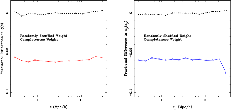
We first show the effect of weighting by sky completeness on the 2PCF in Figure 14. We see this sample shows an approximately $6\%$ offset in both redshift and projected space at all scales below $30\;h^{-1}\mathrm{Mpc}$ if the weights are unaccounted for (see solid lines in both panels). To demonstrate the validity of this test, we have re-measured the exact same galaxy data but randomly shuffled the weights which shows no fractional difference (dotted lines).

Figure 15.— The effects of correcting for sky completeness in the reduced 3PCF. The $Q_{cw}$ denotes the completeness weighted (corrected) quantity. The effect for both redshift space (red, x-marks) and projected space (blue, open circles) measurements are described by the absolute difference (left) and the fractional effect (right). Not accounting for sky completeness introduces a systematic offset that varies by scale, which can be seen in the left panel. The projected measurements appear more sensitive to sky completeness than redshift space ones.

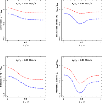
We investigate the effects of neglecting sky completeness on the reduced 3PCF in Figure 15, where we show both the absolute difference (left column) and fractional effect (right). We notice a systematic offset that increases with scale in both redshift and projected measurements. On larger scales ($r_{1}=9\;h^{-1}\mathrm{Mpc}$), we find about a 12% deviation in redshift space and almost 20% difference for projected space, showing more sensitivity to completeness weighting than the 2PCF. We estimate the uncertainties in these measurements from $30$ jackknife samples at approximately 12% and 17% respectively, and we conclude that sky completeness must be considered for accurate 3PCF measurements.

A.3. Effects of Binning

The choice of binning scheme affects measurements and covariance matrices of the configuration dependence in the 3PCF. To be specific, we refer to the choice of bin-size as well as their spacing by “binning scheme”. For the 2PCF, the most common scheme is to use log spaced bins in $r$ to account for the dynamic range of scales and power law dependence of the 2PCF. In this scheme, bins at larger $r$ correspond to larger bin-widths. When we measure $Q(\theta)$, the angular bins are closely packed over a much smaller scale range making a choice of log spaced bins impractical. If the bin-size is too large, we notice an attenuation or averaging out of the configuration dependence. On the other hand, if the bin-size is too small, we do not resolve the measurement nor the covariance. Both the sample size and number density will impact the efficiency of a binning scheme. Even if we find an acceptable choice for one sample, it might show different effects on another sample. This effect remains more dramatic for the 3PCF due to the larger parameter space of potential configurations.

Naively, for a given data set of size $N$, we expect the number of available triplets (i.e. $N^{3}$) to be much larger than pairs ($N^{2}$). However, the configuration dependence of the 3PCF is a function of three dependent variables. Any specific configuration represents a tiny slice through the available data, making the 3PCF much harder to determine. For a rough idea, we can compare the number of triplets to the number of pairs for a specific 3PCF configuration. For a choice of binning scheme with no overlap for the $r_{1}=9\;h^{-1}\mathrm{Mpc}$ triangles, we find that approximately $1$ in every $1000$ pairs contribute to the 2PCF for the denominator of $Q_{proj}(\theta)$. For the 3PCF (the numerator), only $1$ in $67,000,000$ contribute. Even if we consider that the 3PCF scales as the square of the 2PCF (i.e. $\zeta\propto\xi^{2}$), we notice the triplet count in the 3PCF remains smaller by a factor of $\sim 67$.

The impact of bin-size has only recently been addressed in the literature (see Gaztañaga and Scoccimarro 2005). We believe this remained unresolved for two main reasons (1) the availability of large datasets to statistically determine finely binned higher order moments, and (2) the computational complexity of calculating them. For a small data sample, it may not be possible to measure the 3PCF with small enough bins. This is not the case with our SDSS samples. Most methods of estimation solve the computational complexity by performing counts after pre-gridding the data, thereby imposing a bin-size effect. While this can help mask the effect, it does not hide it entirely. Gaztañaga and Scoccimarro (2005) comment on the effect of bin-size using a pre-gridding technique by using a sufficiently fine grid. Our estimation of correlation functions uses an efficient counting algorithm to yield exact counts, so we do not need to pre-grid our data. At large scales, measurements using a sufficiently fine pre-gridding technique and those with an exact count converge. At small scales, pre-gridding becomes less effective at reducing the computational expense and may become prohibitively expensive.

Gaztañaga and Scoccimarro (2005) suggest a good test of bin-size is to measure the small scale configuration dependence of the reduced 3PCF in redshift space. Redshift distortions produce elongated finger-of-god structures, which should significantly amplify the signal of collapsed triangles at $\theta=0$ and $\theta=\pi$. This characteristic “U-shape” will not be present if the bin-size is too large, since the finger-of-god structures are effectively averaged over. For the 3PCF, we must consider the bin-size in three parameters, i.e. each side of the triplet. In figure 16, we show three choices of bin-size in $\theta$ when two sides of the triangle ($r_{1},r_{2}$) are tightly constrained ($\pm 0.1\;h^{-1}\mathrm{Mpc}$). Even with large bins in $\theta$, all measurements equivalently show configuration dependence, demonstrating the importance of bin-size for $r_{1}$ and $r_{2}$. We also show a measurement with “large bins”, constructed to match those used in Nichol et al. (2006) where the first side of the triangle ($r_{1}$) varies by $\pm 0.5\;h^{-1}\mathrm{Mpc}$. The larger bin-size completely masks the configuration dependence expected from the redshift distortions.

Figure 16.— We show the reduced 3PCF on a subset of SDSS data. At small scales, we expect the redshift space distortions to cause a “U-shape” signal due to elongated fingers-of-god. This plot illustrates that small binning ($\pm 0.1\;h^{-1}\mathrm{Mpc}$) in the two sides ($r_{1}$ and $r_{2}$) resolves the “U-shape” even with large $\theta$ bins. For comparison, we show “Large Bins” defined to correspond to the binning scheme of Nichol et al. (2006) (i.e. $\pm 0.5\;h^{-1}\mathrm{Mpc}$). The error bars show the combined Poisson errors of the respective counts and signify the statistical significance of the bin-sizes.

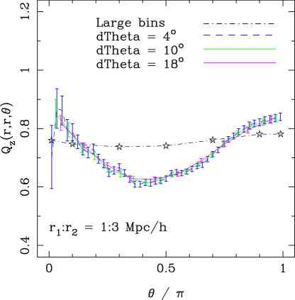
In Figure 17 we extend the comparison of bin-width to the three specific scales that we measure in redshift and projected space. We utilize our fiducial binning scheme, which consists of 15 linear spaced bins in $\theta$ with the bin-width chosen to be a fraction (denoted with $f$) of the scale of the bin midpoint. To be clear, the bin-size for $r_{1}$ and $r_{2}$ also change appropriately with $f$. We show results for $f=0.1,0.2$ and $0.3$ with $1\sigma$ Poisson uncertainties calculated from bin counts. The larger bin-width smooths the configuration dependence at all scales, with a dramatic effect on the $r_{1}=9\;h^{-1}\mathrm{Mpc}$ triangles. This occurs in both redshift and projected space measurements of $Q(\theta)$. Physically, larger bins allow a greater range of configurations to be represented in each bin.

Figure 17.— In our measurements on DR6 data, we adopt a fiducial binning scheme using linear spaced bins in $\theta$ with a bin-size a set fraction of the midpoint. For the three triangle scales of interest, we compare this scheme using three fractional bin-widths on $Q_{z}$ (top row) and $Q_{proj}$ (bottom row): $10$, $20$ and $30$%. The error bars represent Poisson errors on the counts from each bin. Larger bin-width measurements show smaller uncertainties and less configuration dependence. We use the LSTAR galaxy sample from DR6 selected to have $-21.5<M_{r}<-20.5$.

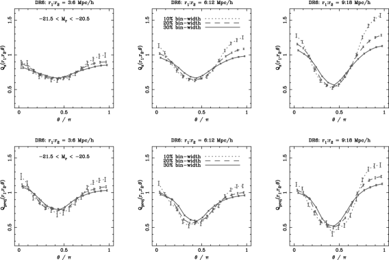
We keep the number of bins fixed (at 15) but vary the bin-width; this results in an increased overlap of configurations, and hence imposes a larger correlation in the covariance between neighboring bins. Basically, the physical overlap is simply larger for equally spaced $\theta$ bins when $\theta$ corresponds to $\sim 0$ or $\sim\pi$. We show the covariance matrices for $Q_{z}(\theta)$ and $Q_{proj}(\theta)$ in Figure 18 for the largest scale ($r_{1}=9\;h^{-1}\mathrm{Mpc}$) and two bin-widths using $f=0.1$ and $0.25$. The significant configuration overlap in $f=0.25$ results in a larger correlation, as we expect. However, we also see increased correlation in non-overlapping bins (see the $\theta\sim 0$ with $\theta\sim\pi$ bins; the top left and bottom right corners).

Figure 18.— For our fiducial binning scheme, we show the covariance matrices for $Q_{z}(\theta)$ (top row) and $Q_{proj}(\theta)$ (bottom row) for the largest triangles with $r_{1}=9\;h^{-1}\mathrm{Mpc}$. The solid, dashed and dotted contours correspond respectively to values of 0.70, 0.85 and 0.99. We use the LSTAR galaxy sample from DR6 ($-21.5<M_{r}<-20.5$).

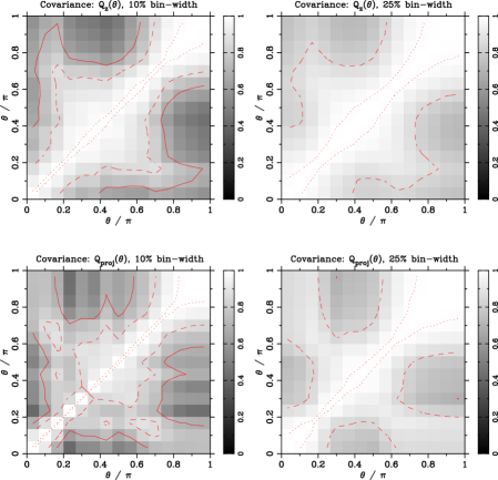
Clearly identified differences due to bin-size are prevalent in both measurements of the reduced 3PCF and its covariance. The general rule of thumb is that smaller bins, assuming they are well resolved, produce more accurate results – but that assumes we properly resolve the covariance.

Appendix B Projected Correlation Functions

The purpose of employing projected correlation functions is to minimize the effects of redshift distortions on clustering measurements. However, we might ask how effective the projected statistic really is. We use the Hubble volume (HV) $N$-body simulations to investigate this question. Since we want to apply our results to observational galaxy surveys, we construct realizations of dark matter (DM) that have the same footprint and volume of an observation galaxy sample. This should incorporate any edge effects or issues of finite volume that are also present in galaxy data. We use line-of-sight peculiar velocities to create a redshift space distribution of DM. In a few cases, we compare this to a similar distribution without any redshift distortions, which we call real space. Two important decisions need to be made when using projected measurements: (1) how large of $\Delta\pi$ bins do we use to integrate over and (2) what is the maximum line-of-sight distance for the integration ($\pi_{\mathrm{max}}$).

The first question stated above is relatively easy to address. We want to choose bins of $\Delta\pi$ that remain small enough to prevent a smoothing bias. In the left panel of Figure 19, we show the anisotropy introduced by redshift distortions on the 2PCF, the $r_{p}-\pi$ diagram, within our HV test sample. Using these data, we calculate the projected 2PCF by integrating to $\pi_{\mathrm{max}}=40\;h^{-1}\mathrm{Mpc}$ with different values of $\Delta\pi$. We compare each with the fiducial measurement using $\Delta\pi=2\;h^{-1}\mathrm{Mpc}$, and show the fractional difference in Figure 19. We notice a very small effect, and the largest deviation appears at small projected separation where $\xi(r_{p},\pi)$ changes rapidly. The systematic effect remains below the 2% level even with bins as wide as $\Delta\pi=20\;h^{-1}\mathrm{Mpc}$.

Figure 19.— On the left we show the $r_{p}-\pi$ diagram from the 2PCF on dark matter particles from the Hubble Volume simulation, using a grid of $2\;h^{-1}\mathrm{Mpc}$ in both $r_{p}$ and $\pi$. The HV particles are trimmed to match the same volume and footprint of SDSS data, with velocities used to construct radial redshift distortions. The red (solid) lines are contours of a specific value of the CF, $\xi(r_{p},\pi)$, with values of $3,2,1,0.6,0.4,0.2,0.1,0.07,0.04$ with the yellow highlighted one corresponding to $\xi(r_{p},\pi)=1$ . The blue (dot-dashed) semi-circles show a perfect isotropic correlation for comparison. On the right, we depict the accuracy of the $w_{p}(r_{p})$ integration using different sized $\pi$ bins, which we show as a function of projected scale ($r_{p}$). We obtain the “truth” value by comparing to a fiducial $\Delta\pi=2\;h^{-1}\mathrm{Mpc}$, and our $\pi_{\mathrm{max}}=40\;h^{-1}\mathrm{Mpc}$. We show the 1% level of accuracy with the dashed line.

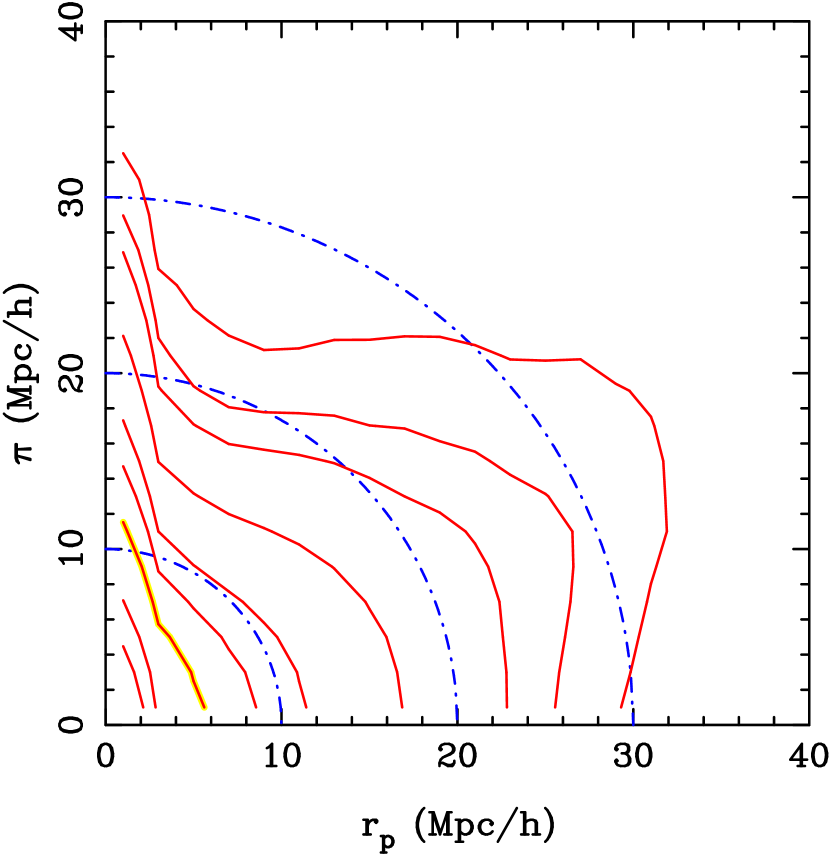
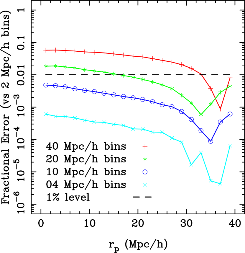
The second question remains more subtle: what is an appropriate $\pi_{\mathrm{max}}$? Formally, we might prefer to keep $\pi_{\mathrm{max}}=\infty$, which preserves the property that a power law spatial correlation function $\xi$ produces a power law projected 2PCF $w_{p}$. Realistically, galaxy samples represent finite volumes and the correlation function can only be well estimated to a certain maximum distance. We want to keep our $\pi_{\mathrm{max}}$ well below this limit, lest we dilute our signal. On the other hand, we want $\pi_{\mathrm{max}}$ be large enough to (re-)capture clustering strength lost due to redshift distortions. We compute $w_{p}(r_{p})$ using two same volume realizations of DM, one in real space (no distortions) and one in redshift space, which we compare in Figure 20. We expand $\pi_{\mathrm{max}}$ to range between $20$ and $80\;h^{-1}\mathrm{Mpc}$. We see several interesting features. First, both real and redshift space $w_{p}(r_{p})$ are roughly power laws, with the strongest power corresponding to the largest $\pi_{\mathrm{max}}$. We expected this, as the projected 2PCF has units of distance, a larger integration equates to a higher functional value. We notice a much smaller difference between the smallest and largest $\pi_{\mathrm{max}}$ in redshift space. This is a result of the large scale infall (Kaiser 1987), as clustering strength is compressed to smaller line-of-sight separation which we see in Figure 19. Examining the fractional difference between real and redshift space measurements, we find a higher $\pi_{\mathrm{max}}$ does what we expect in reducing the difference between real and redshift space $w_{p}(r_{p})$ measurements. However, we also see that different values of $\pi_{\mathrm{max}}$ dramatically changes the 2PCF from the “ideal case”, inducing a systematic difference which can range from right below the 10% level at $r_{p}=10;\pi_{\mathrm{max}}=80\;h^{-1}\mathrm{Mpc}$ to 80% at the largest scales and smallest $\pi_{\mathrm{max}}$. Finally, we conclude that even at $\pi_{\mathrm{max}}=80\;h^{-1}\mathrm{Mpc}$ the effects of redshift distortions cannot be completely negated by the projected 2PCF.

Figure 20.— We show the projected 2PCF, $w_{p}(r_{p})$, for dark matter particles in the Hubble Volume simulation both in real space (top left panel), redshift space (top right panel), the absolute difference due to redshift distortions (bottom left panel), and the fractional difference (bottom right panel). The different curves correspond to different $\pi_{\mathrm{max}}$ integrations, as denoted. We estimate $w_{p}(r_{p})$ by integrating in bins of $\Delta\pi=5\;h^{-1}\mathrm{Mpc}$. The legend in the top two panels denotes the maximum $\pi_{\mathrm{max}}$ used for each calculation, such that “pi20” corresponds to $\pi_{\mathrm{max}}=20\;h^{-1}\mathrm{Mpc}$, etc.

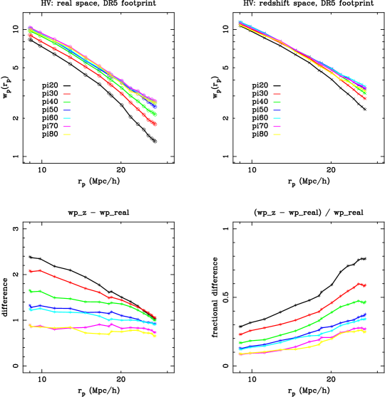
We extend the investigation to the reduced 3PCF, using the two largest triangle configurations ($r_{1}=6$ and $9\;h^{-1}\mathrm{Mpc}$). Since $Q(\theta)$ is normalized by the respective 2PCF, we expect the same amplitude between spatial and projected measurements and can compare measurements on real observed galaxy samples. We show the measurements on an SDSS sample where we measure $Q(\theta)$ in redshift space and projected with $\pi_{\mathrm{max}}=20,$ $30$ and $40\;h^{-1}\mathrm{Mpc}$ in Figure 21. For observational galaxies, it appears that $Q_{proj}$ recovers some configuration dependence with larger $\pi_{\mathrm{max}}$. The $r_{1}=9\;h^{-1}\mathrm{Mpc}$ triangles show decreased amplitude perpendicular configurations and we note the “splitting” of collapsed triangles ($\theta\sim 0$) in the smaller triangles. In both cases, a decreased $\pi_{\mathrm{max}}$ yields a $Q(\theta)$ that approaches the redshift space measurement, in agreement with our expectations.

Figure 21.— We show the reduced 3PCF, $Q(\theta)$, on a galaxy sample from SDSS DR5 at our two largest triangle scales: $r_{1}=6$ & $9\;h^{-1}\mathrm{Mpc}$. We compare three different values of $\pi_{\mathrm{max}}$, namely $20,30$ and $40\;h^{-1}\mathrm{Mpc}$ with the spatial reduced 3PCF in redshift space. We note the lower values of $\pi_{\mathrm{max}}$ tend toward the redshift space measurement, but emphasize that it is a minor effect at these scales.

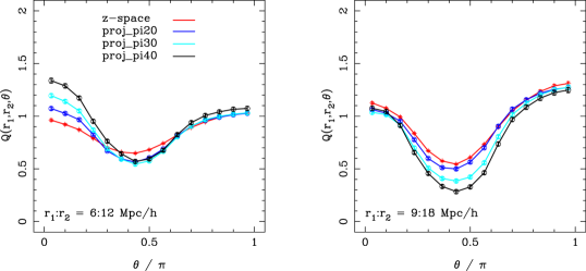
Overall, we conclude that the projected correlation function reduces the impact of redshift distortions on measurements of clustering. However, the projected statistic does not completely remove effects of the distortions for any of practical values of $\pi_{\mathrm{max}}$ that we might use. Our results suggest a larger $\pi_{\mathrm{max}}$ might further minimize redshift distortions but a more thorough investigation is required to disentangle the systematics (for example, we integrate the projected 3PCF with a single bin of $\pi_{\mathrm{max}}$ width which we would have to investigate). Since the computational efficiency of estimating the 3PCF decreases dramatically with increased $\pi_{\mathrm{max}}$, we choose to use $\pi_{\mathrm{max}}=20\;h^{-1}\mathrm{Mpc}$ for our measurements. This choice should be sufficient to minimize some effects of redshift distortions, remaining most effective at small scales where it will recapture clustering strength lost from the non-linear collapse in dense regions (the fingers-of-god).

References

- Tegmark et al. (2004) M. Tegmark, M. R. Blanton, M. A. Strauss, F. Hoyle, D. Schlegel, R. Scoccimarro, M. S. Vogeley, D. H. Weinberg, I. Zehavi, A. Berlind, et al., ApJ 606, 702 (2004), arXiv:astro-ph/0310725.
- Cole et al. (2005) S. Cole, W. J. Percival, J. A. Peacock, P. Norberg, C. M. Baugh, C. S. Frenk, I. Baldry, J. Bland-Hawthorn, T. Bridges, R. Cannon, et al., MNRAS 362, 505 (2005), arXiv:astro-ph/0501174.
- Eisenstein et al. (2005) D. J. Eisenstein, I. Zehavi, D. W. Hogg, R. Scoccimarro, M. R. Blanton, R. C. Nichol, R. Scranton, H. Seo, M. Tegmark, Z. Zheng, et al., ApJ 633, 560 (2005), arXiv:astro-ph/0501171.
- Tegmark et al. (2006) M. Tegmark, D. J. Eisenstein, M. A. Strauss, D. H. Weinberg, M. R. Blanton, J. A. Frieman, M. Fukugita, J. E. Gunn, A. J. S. Hamilton, G. R. Knapp, et al., Phys. Rev. D 74, 123507 (2006), arXiv:astro-ph/0608632.
- Sánchez et al. (2009) A. G. Sánchez, M. Crocce, A. Cabré, C. M. Baugh, and E. Gaztañaga, MNRAS 400, 1643 (2009), 0901.2570.
- Spergel et al. (2007) D. N. Spergel, R. Bean, O. Doré, M. R. Nolta, C. L. Bennett, J. Dunkley, G. Hinshaw, N. Jarosik, E. Komatsu, L. Page, et al., ApJS 170, 377 (2007), arXiv:astro-ph/0603449.
- Komatsu et al. (2009) E. Komatsu, J. Dunkley, M. R. Nolta, C. L. Bennett, B. Gold, G. Hinshaw, N. Jarosik, D. Larson, M. Limon, L. Page, et al., ApJS 180, 330 (2009), 0803.0547.
- York et al. (2000) D. G. York, J. Adelman, J. E. Anderson, Jr., S. F. Anderson, J. Annis, N. A. Bahcall, J. A. Bakken, R. Barkhouser, S. Bastian, E. Berman, et al., AJ 120, 1579 (2000), arXiv:astro-ph/0006396.
- Stoughton et al. (2002) C. Stoughton, R. H. Lupton, M. Bernardi, M. R. Blanton, S. Burles, F. J. Castander, A. J. Connolly, D. J. Eisenstein, J. A. Frieman, G. S. Hennessy, et al., AJ 123, 485 (2002).
- Peebles (1980) P. J. E. Peebles, The large-scale structure of the universe (1980).
- Zehavi et al. (2004) I. Zehavi, D. H. Weinberg, Z. Zheng, A. A. Berlind, J. A. Frieman, R. Scoccimarro, R. K. Sheth, M. R. Blanton, M. Tegmark, H. J. Mo, et al., ApJ 608, 16 (2004), arXiv:astro-ph/0301280.
- Zehavi et al. (2005) I. Zehavi, Z. Zheng, D. H. Weinberg, J. A. Frieman, A. A. Berlind, M. R. Blanton, R. Scoccimarro, R. K. Sheth, M. A. Strauss, I. Kayo, et al., ApJ 630, 1 (2005), arXiv:astro-ph/0408569.
- Zehavi et al. (2010) I. Zehavi, Z. Zheng, D. H. Weinberg, M. R. Blanton, and S. collaboration, ApJ pp. ??–?? (2010).
- Bernardeau et al. (2002) F. Bernardeau, S. Colombi, E. Gaztañaga, and R. Scoccimarro, Phys. Rep. 367, 1 (2002), arXiv:astro-ph/0112551.
- Zheng and Weinberg (2007) Z. Zheng and D. H. Weinberg, ApJ 659, 1 (2007), arXiv:astro-ph/0512071.
- Kulkarni et al. (2007) G. V. Kulkarni, R. C. Nichol, R. K. Sheth, H. Seo, D. J. Eisenstein, and A. Gray, MNRAS 378, 1196 (2007), arXiv:astro-ph/0703340.
- Sefusatti and Scoccimarro (2005) E. Sefusatti and R. Scoccimarro, Phys. Rev. D 71, 063001 (2005), arXiv:astro-ph/0412626.
- Szapudi (2009) I. Szapudi, in Data Analysis in Cosmology, edited by V. J. Martinez, E. Saar, E. M. Gonzales, & M. J. Pons-Borderia (2009), vol. 665 of Lecture Notes in Physics, Berlin Springer Verlag, pp. 457–+.
- Jing and Börner (2004) Y. P. Jing and G. Börner, ApJ 607, 140 (2004), arXiv:astro-ph/0311585.
- Wang et al. (2004) Y. Wang, X. Yang, H. J. Mo, F. C. van den Bosch, and Y. Chu, MNRAS 353, 287 (2004), arXiv:astro-ph/0404143.
- Gaztañaga et al. (2005) E. Gaztañaga, P. Norberg, C. M. Baugh, and D. J. Croton, MNRAS 364, 620 (2005), %****␣dr6_3pcf.bbl␣Line␣275␣****arXiv:astro-ph/0506249.
- Kayo et al. (2004) I. Kayo, Y. Suto, R. C. Nichol, J. Pan, I. Szapudi, A. J. Connolly, J. Gardner, B. Jain, G. Kulkarni, T. Matsubara, et al., PASJ 56, 415 (2004), arXiv:astro-ph/0403638.
- Nichol et al. (2006) R. C. Nichol, R. K. Sheth, Y. Suto, A. J. Gray, I. Kayo, R. H. Wechsler, F. Marin, G. Kulkarni, M. Blanton, A. J. Connolly, et al., MNRAS 368, 1507 (2006), arXiv:astro-ph/0602548.
- Verde et al. (2002) L. Verde, A. F. Heavens, W. J. Percival, S. Matarrese, C. M. Baugh, J. Bland-Hawthorn, T. Bridges, R. Cannon, S. Cole, M. Colless, et al., MNRAS 335, 432 (2002), %****␣dr6_3pcf.bbl␣Line␣325␣****arXiv:astro-ph/0112161.
- Pan and Szapudi (2005) J. Pan and I. Szapudi, MNRAS 362, 1363 (2005), arXiv:astro-ph/0505422.
- Hikage et al. (2005) C. Hikage, T. Matsubara, Y. Suto, C. Park, A. S. Szalay, and J. Brinkmann, PASJ 57, 709 (2005), arXiv:astro-ph/0506194.
- Nishimichi et al. (2007) T. Nishimichi, I. Kayo, C. Hikage, K. Yahata, A. Taruya, Y. P. Jing, R. K. Sheth, and Y. Suto, PASJ 59, 93 (2007), arXiv:astro-ph/0609740.
- Fry and Gaztanaga (1993) J. N. Fry and E. Gaztanaga, ApJ 413, 447 (1993), arXiv:astro-ph/9302009.
- Gunn et al. (1998) J. E. Gunn, M. Carr, C. Rockosi, M. Sekiguchi, K. Berry, B. Elms, E. de Haas, Ž. Ivezić, G. Knapp, R. Lupton, et al., AJ 116, 3040 (1998), arXiv:astro-ph/9809085.
- Gunn et al. (2006) J. E. Gunn, W. A. Siegmund, E. J. Mannery, R. E. Owen, C. L. Hull, R. F. Leger, L. N. Carey, G. R. Knapp, D. G. York, W. N. Boroski, et al., AJ 131, 2332 (2006), arXiv:astro-ph/0602326.
- Fukugita et al. (1996) M. Fukugita, T. Ichikawa, J. E. Gunn, M. Doi, K. Shimasaku, and D. P. Schneider, AJ 111, 1748 (1996).
- Smith et al. (2002) J. A. Smith, D. L. Tucker, S. Kent, M. W. Richmond, M. Fukugita, T. Ichikawa, S. Ichikawa, A. M. Jorgensen, A. Uomoto, J. E. Gunn, et al., AJ 123, 2121 (2002), arXiv:astro-ph/0201143.
- Lupton et al. (2001) R. Lupton, J. E. Gunn, Z. Ivezić, G. R. Knapp, and S. Kent, in Astronomical Data Analysis Software and Systems X, edited by F. R. Harnden, Jr., F. A. Primini, and H. E. Payne (2001), vol. 238 of Astronomical Society of the Pacific Conference Series, pp. 269–+.
- Pier et al. (2003) J. R. Pier, J. A. Munn, R. B. Hindsley, G. S. Hennessy, S. M. Kent, R. H. Lupton, and Ž. Ivezić, AJ 125, 1559 (2003), arXiv:astro-ph/0211375.
- Hogg et al. (2001) D. W. Hogg, D. P. Finkbeiner, D. J. Schlegel, and J. E. Gunn, AJ 122, 2129 (2001), arXiv:astro-ph/0106511.
- Ivezić et al. (2004) Ž. Ivezić, R. H. Lupton, D. Schlegel, B. Boroski, J. Adelman-McCarthy, B. Yanny, S. Kent, C. Stoughton, D. Finkbeiner, N. Padmanabhan, et al., Astronomische Nachrichten 325, 583 (2004), arXiv:astro-ph/0410195.
- Tucker et al. (2006) D. L. Tucker, S. Kent, M. W. Richmond, J. Annis, J. A. Smith, S. S. Allam, C. T. Rodgers, J. L. Stute, J. K. Adelman-McCarthy, J. Brinkmann, et al., Astronomische Nachrichten 327, 821 (2006), arXiv:astro-ph/0608575.
- Padmanabhan et al. (2008) N. Padmanabhan, D. J. Schlegel, D. P. Finkbeiner, J. C. Barentine, M. R. Blanton, H. J. Brewington, J. E. Gunn, M. Harvanek, D. W. Hogg, Ž. Ivezić, et al., ApJ 674, 1217 (2008), arXiv:astro-ph/0703454.
- Strauss et al. (2002) M. A. Strauss, D. H. Weinberg, R. H. Lupton, V. K. Narayanan, J. Annis, M. Bernardi, M. Blanton, S. Burles, A. J. Connolly, J. Dalcanton, et al., AJ 124, 1810 (2002), arXiv:astro-ph/0206225.
- Blanton et al. (2003) M. R. Blanton, H. Lin, R. H. Lupton, F. M. Maley, N. Young, I. Zehavi, and J. Loveday, AJ 125, 2276 (2003), arXiv:astro-ph/0105535.
- Blanton et al. (2005a) M. R. Blanton, D. J. Schlegel, M. A. Strauss, J. Brinkmann, D. Finkbeiner, M. Fukugita, J. E. Gunn, D. W. Hogg, Ž. Ivezić, G. R. Knapp, et al., AJ 129, 2562 (2005a), arXiv:astro-ph/0410166.
- Adelman-McCarthy et al. (2008) J. K. Adelman-McCarthy, M. A. Agüeros, S. S. Allam, C. Allende Prieto, K. S. J. Anderson, S. F. Anderson, J. Annis, N. A. Bahcall, C. A. L. Bailer-Jones, I. K. Baldry, et al., ApJS 175, 297 (2008), 0707.3413.
- Zehavi et al. (2002) I. Zehavi, M. R. Blanton, J. A. Frieman, D. H. Weinberg, H. J. Mo, M. A. Strauss, S. F. Anderson, J. Annis, N. A. Bahcall, M. Bernardi, et al., ApJ 571, 172 (2002), arXiv:astro-ph/0106476.
- Baldry et al. (2004) I. K. Baldry, K. Glazebrook, J. Brinkmann, Ž. Ivezić, R. H. Lupton, R. C. Nichol, and A. S. Szalay, ApJ 600, 681 (2004), arXiv:astro-ph/0309710.
- Colberg et al. (2000) J. M. Colberg, S. D. M. White, N. Yoshida, T. J. MacFarland, A. Jenkins, C. S. Frenk, F. R. Pearce, A. E. Evrard, H. M. P. Couchman, G. Efstathiou, et al., MNRAS 319, 209 (2000), arXiv:astro-ph/0005259.
- Evrard et al. (2002) A. E. Evrard, T. J. MacFarland, H. M. P. Couchman, J. M. Colberg, N. Yoshida, S. D. M. White, A. Jenkins, C. S. Frenk, F. R. Pearce, J. A. Peacock, et al., ApJ 573, 7 (2002), arXiv:astro-ph/0110246.
- Jackson (1972) J. C. Jackson, MNRAS 156, 1P (1972).
- Sargent and Turner (1977) W. L. W. Sargent and E. L. Turner, ApJ 212, L3 (1977).
- Hamilton (1998) A. J. S. Hamilton, in The Evolving Universe, edited by D. Hamilton (1998), vol. 231 of Astrophysics and Space Science Library, pp. 185–+.
- Kaiser (1987) N. Kaiser, MNRAS 227, 1 (1987).
- Szapudi and Szalay (1998) S. Szapudi and A. S. Szalay, ApJ 494, L41+ (1998).
- Landy and Szalay (1993) S. D. Landy and A. S. Szalay, ApJ 412, 64 (1993).
- Gardner et al. (2007) J. P. Gardner, A. Connolly, and C. McBride, in Astronomical Data Analysis Software and Systems XVI, edited by R. A. Shaw, F. Hill, & D. J. Bell (2007), vol. 376 of Astronomical Society of the Pacific Conference Series, pp. 69–+.
- Moore et al. (2001) A. W. Moore, A. J. Connolly, C. Genovese, A. Gray, L. Grone, N. I. Kanidoris, R. C. Nichol, J. Schneider, A. S. Szalay, I. Szapudi, et al., in Mining the Sky, edited by A. J. Banday, S. Zaroubi, & M. Bartelmann (2001), pp. 71–+.
- Gray et al. (2004) A. G. Gray, A. W. Moore, R. C. Nichol, A. J. Connolly, C. Genovese, and L. Wasserman, in Astronomical Data Analysis Software and Systems (ADASS) XIII, edited by F. Ochsenbein, M. G. Allen, & D. Egret (2004), vol. 314 of Astronomical Society of the Pacific Conference Series, pp. 249–+.
- Marín et al. (2008) F. A. Marín, R. H. Wechsler, J. A. Frieman, and R. C. Nichol, ApJ 672, 849 (2008), 0704.0255.
- Gaztañaga and Scoccimarro (2005) E. Gaztañaga and R. Scoccimarro, MNRAS 361, 824 (2005), arXiv:astro-ph/0501637.
- Norberg et al. (2009) P. Norberg, C. M. Baugh, E. Gaztañaga, and D. J. Croton, MNRAS 396, 19 (2009), 0810.1885.
- Scranton et al. (2005) R. Scranton, B. Ménard, G. T. Richards, R. C. Nichol, A. D. Myers, B. Jain, A. Gray, M. Bartelmann, R. J. Brunner, A. J. Connolly, et al., ApJ 633, 589 (2005), arXiv:astro-ph/0504510.
- Totsuji and Kihara (1969) H. Totsuji and T. Kihara, PASJ 21, 221 (1969).
- Cooray and Sheth (2002) A. Cooray and R. Sheth, Phys. Rep. 372, 1 (2002), arXiv:astro-ph/0206508.
- Scoccimarro (2000) R. Scoccimarro, ApJ 544, 597 (2000), arXiv:astro-ph/0004086.
- Smith et al. (2008) R. E. Smith, R. K. Sheth, and R. Scoccimarro, Phys. Rev. D 78, 023523 (2008), 0712.0017.
- Chen and Szapudi (2006) G. Chen and I. Szapudi, ApJ 647, L87 (2006), arXiv:astro-ph/0606394.
- Bardeen et al. (1986) J. M. Bardeen, J. R. Bond, N. Kaiser, and A. S. Szalay, ApJ 304, 15 (1986).
- Gott et al. (2005) J. R. I. Gott, M. Jurić, D. Schlegel, F. Hoyle, M. Vogeley, M. Tegmark, N. Bahcall, and J. Brinkmann, ApJ 624, 463 (2005), arXiv:astro-ph/0310571.
- Gerke et al. (2007) B. F. Gerke, J. A. Newman, S. M. Faber, M. C. Cooper, D. J. Croton, M. Davis, C. N. A. Willmer, R. Yan, A. L. Coil, P. Guhathakurta, et al., MNRAS 376, 1425 (2007), arXiv:astro-ph/0608569.
- Blanton et al. (2005b) M. R. Blanton, D. Eisenstein, D. W. Hogg, D. J. Schlegel, and J. Brinkmann, ApJ 629, 143 (2005b), arXiv:astro-ph/0310453.
- Azzaro et al. (2007) M. Azzaro, S. G. Patiri, F. Prada, and A. R. Zentner, MNRAS 376, L43 (2007), arXiv:astro-ph/0607139.
- Colless et al. (2001) M. Colless, G. Dalton, S. Maddox, W. Sutherland, P. Norberg, S. Cole, J. Bland-Hawthorn, T. Bridges, R. Cannon, C. Collins, et al., MNRAS 328, 1039 (2001), arXiv:astro-ph/0106498.
- Kerscher et al. (2000) M. Kerscher, I. Szapudi, and A. S. Szalay, ApJ 535, L13 (2000), arXiv:astro-ph/9912088.
- Adelman-McCarthy et al. (2007) J. K. Adelman-McCarthy, M. A. Agüeros, S. S. Allam, K. S. J. Anderson, S. F. Anderson, J. Annis, N. A. Bahcall, C. A. L. Bailer-Jones, I. K. Baldry, J. C. Barentine, et al., ApJS 172, 634 (2007), arXiv:0707.3380.