Cosmological parameter constraints from SDSS luminous red galaxies: a new treatment of large-scale clustering.

Abstract

We apply a new model for the spherically averaged correlation function at large pair separations to the measurement of the clustering of luminous red galaxies (LRGs) made from the SDSS by Cabre & Gaztañaga (2009a). Our model takes into account the form of the BAO peak and the large scale shape of the correlation function. We perform a Monte Carlo Markov chain analysis for different combinations of datasets and for different parameter sets. When used in combination with a compilation of the latest CMB measurements, the LRG clustering and the latest supernovae results give constraints on cosmological parameters which are comparable and in remarkably good agreement, resolving the tension reported in some studies. The best fitting model in the context of a flat, $\Lambda$-CDM cosmology is specified by $\Omega_{\rm m}=0.261\pm 0.013$, $\Omega_{\rm b}=0.044\pm 0.001$, $n_{\rm s}=0.96\pm 0.01$, $H_{0}=71.6\pm 1.2\,{\rm km}\,{\rm s}^{-1}\,{\rm Mpc}^{-1}$ and $\sigma_{8}=0.80\pm 0.02$. If we allow the time-independent dark energy equation of state parameter to vary, we find results consistent with a cosmological constant at the $5\%$ level using all data sets: $w_{\rm DE}=-0.97\pm 0.05$. The large scale structure measurements by themselves can constrain the dark energy equation of state parameter to $w_{\rm DE}=-1.05^{+0.16}_{-0.15}$, independently of CMB or supernovae data. We do not find convincing evidence for an evolving equation of state. We provide a set of “extended distance priors” that contain the most relevant information from the CMB power spectrum and the shape of the LRG correlation function which can be used to constrain dark energy models and spatial curvature. Our model should provide an accurate description of the clustering even in much larger, forthcoming surveys, such as those planned with NASA’s JDEM or ESA’s Euclid mission.

1 Introduction

The acoustic peaks imprinted on the temperature power spectrum of the cosmic microwave background (CMB) have now been measured with impressive precision by a number of experiments (Lee et al., 2001; Bennet et al., 2003; Hinshaw et al., 2003, 2007, 2009; Jones et  al., 2006; Reichardt et al., 2009). These observations place tight constraints on the values of many of the fundamental cosmological parameters. With the fifth year of integration from the WMAP satellite there is seemingly little room left for any deviation from the basic $\Lambda$CDM model (Dunkley et al., 2009; Komatsu et al., 2009). However, degeneracies exist between some parameters which cannot be broken by CMB data alone (e.g. (Bond et al., 1997; Efstathiou & Bond, 1999; Bridle et al., 2003). Perhaps the two most important examples are the curvature of the Universe and the equation of state of the dark energy, $w_{\rm DE}=P_{\rm DE}/\rho_{\rm DE}$, where $P_{\rm DE}$ is the pressure of the dark energy and $\rho_{\rm DE}$ is its density. Meaningful constraints cannot be obtained on these parameters using CMB data in isolation.

The full potential of the CMB measurements is realized when these data are combined with other observations, such as the Hubble diagram of type Ia supernovae and the large scale structure of the Universe as traced by galaxies (Riess et al., 1998; Perlmutter et al., 1999; Efstathiou et al., 2002; Percival et al., 2002; Spergel et al., 2003; Riess et al., 2004; Tegmark et al., 2004; Seljak et al., 2005; Sánchez et al., 2006; Astier et al., 2006; Seljak et al., 2006; Wang & Mukherjee, 2006; Wood-Vasey et al., 2007; Spergel et al., 2007; Komatsu et al., 2009; Okumura et al., 2008; Xia et al., 2008; Ferramacho et al., 2009). These complementary data sets come from the late Universe compared with the CMB data, and the interpretation of the observations is more complicated and controversial.

Type Ia supernovae (SNe) have been proposed as standard candles which can probe the luminosity distance - redshift relation. The first strong evidence in support of a cosmological constant came from combining the SNe data with CMB measurements (Riess et al., 1998; Perlmutter et al., 1999). The type Ia Hubble diagram has come under intense scrutiny to uncover any hint of non-standardness arising from the nature of the host galaxy, possible evolution with redshift or variation in dust extinction (Sullivan et al., 2003; Gallagher et al., 2005; Ellis et al., 2008; Howell et al., 2009). A recent joint analysis of SNe from different datasets suggests that the systematic error on the equation of state parameter from a joint CMB and SNe analysis is comparable to the size of the random error (Kowalski et al., 2008).

The power spectrum of galaxy clustering has also been used in combination with CMB data (e.g. Percival et al. 2002). According to the standard lore, the galaxy power spectrum on large scales is expected to have a simple relation to the underlying dark matter spectrum. Moreover, the shape of the spectrum is believed to closely follow that expected in linear perturbation theory for the matter, which can be readily computed given a set of values for the cosmological parameters. However, with the availability of improving measurements and more refined modelling of the galaxy power spectrum it has become clear that this simple picture is no longer sufficiently accurate to describe the data. Additional levels of modelling of the deviations from linear theory have to be incorporated into the analysis. These include empirical models of the nonlinear distortion of the power spectrum (Smith et al., 2003) and possible scale dependent biases between the clustering of galaxies and mass (Cole et al., 2005; Hamann et al., 2008; Cresswell & Percival, 2009). Recent studies have cast doubt on the accuracy of these prescriptions (Sánchez & Cole, 2008; Reid et al., 2008). In principle, if the simple models described the form of the observed power spectrum, then the power spectra measured from different galaxy samples should yield equivalent constraints on cosmological parameters. However, Sánchez & Cole (2008) found a fundamental difference in the shapes of the galaxy power spectra measured from the two-degree galaxy redshift survey and the Sloan Digital Sky Survey, after attempting to correct the measured spectra. These authors found that the red selection of the SDSS galaxies results in a strong scale dependent bias (see also Swanson et al., 2008). Similar scale dependent effects have been seen in the power spectrum of dark matter haloes and galaxies modelled in simulations (Smith et al., 2007; Angulo et al., 2008).

Recent analyses have not attempted to model the overall shape or amplitude of the power spectrum, as a consequence of the difficulties described above in interpreting the results from different samples. Instead, attention has shifted to a pattern of oscillatory features called the baryonic acoustic oscillations (BAO), which are imprinted on the matter power spectrum. These features have been advocated as a standard ruler which can be used to measure the distance-redshift relation, and hence constrain the dark energy equation of state (Blake & Glazebrook, 2003; Hu & Haiman, 2003; Linder et al., 2003; Seo & Eisenstein, 2003; Wang, 2006; Guzik et al., 2007; Seo & Eisenstein, 2007; Seo et al., 2008). The BAO arise from oscillations in the baryon-photon fluid prior to matter-radiation decoupling. This phenomenon gives rise to the peaks seen in the power spectrum of temperature fluctuations in the CMB. In the matter power spectrum, the oscillations have a much smaller amplitude as baryons only account for around 20 per cent of the total matter density of the Universe. Furthermore, the oscillations in the matter spectrum are out of phase with those in the CMB (Sugiyama, 1995; Eisenstein & Hu, 1998, 1999; Meiksin et al., 1999). The oscillation scale is related to the size of the sound horizon at recombination, which can be measured with high accuracy from the CMB (Komatsu et al., 2009). The apparent size of the BAO ruler depends upon the parameters $w_{\rm DE}$ and $\Omega_{k}$, as these determine the angular diameter distance out to a given redshift. In practice, the BAO are not precisely a standard ruler at the level of precision demanded for their interpretation in future surveys. Nevertheless, by modelling the appearance of the BAO accurately, they are still a valuable probe of cosmological parameters (Sánchez et al., 2008; Smith et al., 2008). Careful simulation work and modelling has shown that techniques can be developed which can overcome long-wavelength gradients in the power spectrum to yield robust constraints on the BAO using the galaxy power spectrum (Percival et al., 2007b; Smith et al., 2007; Angulo et al., 2008; Crocce & Scoccimarro, 2008; Takahasi et al., 2008; Seo et al., 2008).

The BAO signal has been detected in both the 2dFGRS and SDSS surveys (Cole et al., 2005; Eisenstein et al., 2005). The most powerful BAO measurements currently come from samples of luminous red galaxies (LRGs) (Cole et al., 2005; Hütsi, 2006; Padmanabhan et al., 2007; Percival et al., 2007b, c; Okumura et al., 2008; Cabre & Gaztañaga, 2009a; Gaztañaga et al., 2008b; Martinez et al., 2009). Detections at a lower significance have also been reported using galaxy clusters (Hütsi, 2007; Estrada et al., 2009). The imprint of these features has even been found in the three point function of LRGs (Gaztañaga et al., 2008a). Despite this rapid progress, the conclusions drawn from measurements of the BAO remain unclear. For example, Percival et al. (2007c) analysed the BAO signal in a joint galaxy sample drawn from the Sloan Digital Sky Survey (SDSS) data release five (DR5) and the two-degree Field Galaxy Redshift Survey (2dFGRS). Ignoring the information from the amplitude and long-wavelength shape of the power spectrum, and simply isolating the BAO, the results of Percival et al. showed a 2.4$\sigma$ discrepancy with the distance measurements inferred from the supernovae type Ia (SN) data by Astier et al. (2006), signaling a possible problem in the modelling of the BAO data, or a challenge to the $\Lambda$CDM model.

Much theoretical work has been devoted to uncovering scale dependent effects in the BAO and in improving the modelling of the signal in galaxy surveys (Angulo et al., 2005; Huff et al., 2007; Smith et al., 2007; Angulo et al., 2008; Smith et al., 2008; Crocce & Scoccimarro, 2008; Seo et al., 2008; Desjacques, 2008). In order to realize the full potential of the BAO technique as a cosmological probe it is essential to quantify any systematics in the signal and to understand how the measurements relate to cosmological parameters. First, let us debunk some possible preconceptions about BAO. As we have remarked above, the BAO are not precisely a standard ruler. In the correlation function, the Fourier transform of the power spectrum, the BAO appear as a broad peak at large pair separations (Matsubara, 2004). Sánchez et al. (2008) showed that even in linear perturbation theory, the maximum of the BAO peak in correlation function does not coincide with the sound horizon scale at the percent level of accuracy required to fully exploit the measurements expected from forthcoming galaxy surveys. Furthermore, Smith et al. (2008) and Crocce & Scoccimarro (2008) have shown that both large volume numerical simulations and theoretical predictions based on renormalized perturbation theory (RPT) indicate that the BAO peak in the correlation function is shifted and distorted in a non-trivial manner relative to the prediction of linear perturbation theory. If unaccounted for, these shifts bias the constraints obtained by using the BAO measurements as a standard ruler.

Careful modelling of the correlation function is therefore required to extract the cosmological information encoded in large scale structure. Sánchez et al. (2008) argued that the correlation function is less affected by scale dependent effects than the power spectrum and that a simple model for the correlation function proposed by Crocce & Scoccimarro (2008), based on RPT (Crocce & Scoccimarro, 2006a, b), gives an essentially unbiased measurement of the dark energy equation of state. This means that information from the large scale shape of the correlation function, in addition to the form of the BAO peak, can be used to provide robust constraints on cosmological parameters. The correlation function therefore provides a better constraint on the distance scale than the more conservative, “BAO only” approach required when using the power spectrum (i.e. which requires the long wavelength shape information to be discarded along with the amplitude).

In this paper we apply this new model to the shape of the redshift space correlation function, $\xi(s)$, of the SDSS Data release 6 (DR6) LRGs measured by Cabre & Gaztañaga (2009a). The LRG sample analysed by Cabre & Gaztañaga (2009a) is twice the size of the sample used to make the first detection of the BAO by Eisenstein et al. (2005), and has also yielded the first measurement of the radial BAO signal, which constrains the Hubble parameter (Gaztañaga et al., 2008b). We combine the LRG clustering information with the latest measurements of CMB and SNe data. We focus on the constraints on the dark energy equation of state and the curvature of the Universe, which are the parameters where the extra information from the shape of $\xi(s)$ can dramatically improve upon the CMB only constraints. We also pay special attention to the consistency of the results obtained with different dataset combinations.

The outline of the paper is as follows. In Section 2, we describe the data used in our parameter estimation. In Section 3 we describe the details of our modelling of the shape of the redshift space correlation function and compare it with measurements in N-body simulations. We also set out the different parameter spaces that we study and describe our methodology for parameter estimation. In Section 4 we assess the impact of the details of the parameter estimation technique on the obtained constraints on cosmological parameters. Section 5 presents our main results for the parameter constraints obtained by comparing theoretical models to the CMB data and the correlation function of the SDSS-DR6. In Section 6 we focus on the constraints on certain distance combinations obtained from the shape of $\xi(s)$. We summarize our conclusions in Section 7. Appendix A gives the theoretical motivation for the model we use to describe the correlation function and Appendix B gives the covariance matrix for the distance constraints.

2 The Datasets

Here we describe the different datasets that we use to constrain cosmological parameters. The modelling of the correlation function of luminous red galaxies is described later on in Section 3.2. The datasets described below are used in different combinations to check the consistency of the constraints returned.

2.1 The redshift space correlation function of SDSS-DR6 LRGs: the monopole

Luminous red galaxies (LRGs) are an efficient tracer of the large scale structure of the Universe. These galaxies are selected by color and magnitude cuts designed to identify intrinsically red, bright galaxies using SDSS photometry (see Eisenstein et al 2001 for a complete description of the color cuts). LRGs can be seen out to higher redshifts than galaxies in a simple magnitude limited catalogue, and so map a larger volume of the Universe. LRGs have a low space density compared to $L_{*}$ galaxies, which means that fewer redshifts have to be measured to map out the same volume. The low space density, which translates into a higher shot noise, is compensated for by the stronger than average clustering of LRGs, which maintains the signal-to-noise of the correlation function at a level which can be measured.

Figure 1: The spherically averaged correlation function of LRGs in redshift space. Circles with errorbars show the correlation function used in this paper. The shaded region shows the dispersion in the correlation function obtained when using the new MANGLE mask of Swanson et al. (2008) with different completeness fractions. The dotted line shows the result for the north stripe of DR6. We have also calculated the correlation function for the new DR7 (solid line), estimated using a random catalog generated from a smoothed version of the selection function. The dashed line shows the estimate from DR7 without smoothing. The measurement from Eisenstein et al. (2005) is shown using triangles; note these authors had fewer LRGs and used broader bins.

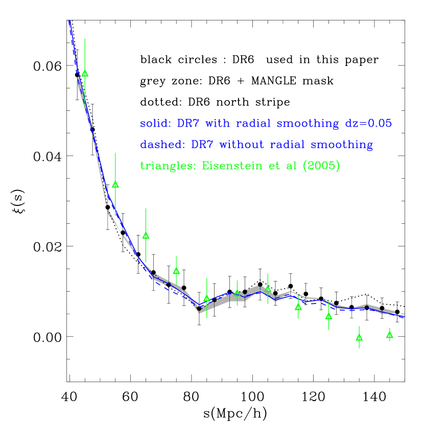
Here we use the measurement of the 2-point correlation function of LRGs in redshift space made by Cabre & Gaztañaga (2009a) shown by the black points in Fig. 1. These authors studied the clustering of LRGs in Data Release 6 (DR6) of the Sloan Digital Sky Survey (SDSS), which has 75 000 LRG galaxies spanning a volume of $1\,h^{-3}\,{\rm Gpc}^{3}$ over the redshift interval $0.15<z<0.47$. The comparison between DR6 and the result of Eisenstein et al. (2005) is plotted in Fig.B4 of Cabre & Gaztañaga (2009a) and Fig. 1; the two results are in good agreement with the DR6 result showing an improvement of a factor of about $\sqrt{2}$ in the size of the errors. Cabre & Gaztañaga (2009a) carried out an extensive series of tests of their measurement of the LRG correlation function. They found that systematic uncertainties in the estimation of the radial selection have a small impact on the results (ie see their figure B2). The adoption of different weighting schemes also produces negligibly small changes (their Fig.B5 and B11). These careful tests indicate that this new estimation of the correlation function is robust and that any possible systematic effects are small compared to the error bars.

Here we recap two aspects of the analysis of Cabre & Gaztañaga (2009a) which are particularly relevant to this paper: the treatment of the survey mask and the estimation of the covariance matrix of the correlation function.

An accurate knowledge of the angular and radial selection of a galaxy catalogue, including the redshift completeness as a function of magnitude and position on the sky, is an essential prerequisite for a measurement of clustering. This information allows the mean density of galaxies in the survey to be estimated. After the release of DR6, Swanson et al. (2008) provided this information in a readily usable form, translating the original mask files extracted from the NYU Value-Added Galaxy Catalog (Blanton et al., 2005), from MANGLE into Healpix format (Gorski et al., 1999). Cabre & Gaztañaga (2009a) describe how they constructed a survey “mask” for LRGs and tested the impact of the mask on clustering measurements using mock catalogues. Using the same techniques, we have also examined the correlation function of LRGs in DR7, which has become available since the submission of Cabre & Gaztañaga (2009a). In Fig. 1, we plot a summary of the possible systematics in the estimation of the correlation function. The estimates corresponding to different versions of the survey mask and different ways of generating a catalogue of random points are in remarkably good agreement with one another. Furthermore, the results from DR6 and DR7 are in excellent agreement; DR7 represents only a modest improvement over DR6. The results of Eisenstein et al. (2005) are plotted in Fig. 1 using triangles. Their estimate is consistent with that of Cabre & Gaztañaga (2009a) within the errors (note that their binning is different, and also, perhaps, their normalisation, due to a small shift which could be attributed to systematics (see Section 2.1.1)). Whilst there is a modest improvement in the parameter constraints on using the DR7 measurement, in line with the incremental change in the number of LRGs and the solid angle covered, we have decided to retain the DR6 measurement in this paper, because the survey mask has been tested more extensively in that case. The DR6 measurement represents a factor of $\sim 2$ more volume than that covered by the LRG sample analyzed by Eisenstein et al. (2005).

Cabre & Gaztañaga (2009a) constructed a covariance matrix for the LRG correlation function using mock catalogues drawn from the MareNostrum Institut de Ciencias del Espacio (MICE) N-body simulations (Fosalba et al., 2008; Crocce et al., 2009). The extremely large volume of this run (box size $7680\,h^{-1}\,{\rm Mpc}$) allowed 216 essentially independent LRG DR6 mocks to be extracted. Cabre & Gaztañaga (2009a) investigated different methods to estimate the error on the correlation function (see their Appendix A). They found that the jackknife error, an internal estimate made from the dataset itself (JK; see Norberg et al. 2008), gave a reasonable match to the diagonal elements of the covariance matrix obtained directly from the 216 mock catalogues. However, the JK estimate of the off-diagonal elements of the covariance matrix is noisier than that obtained from the mocks. In this analysis we construct the full covariance matrix of the measurement from the correlation matrix estimated from mock catalogues of dark matter haloes with similar clustering and abundance to the LRGs, rescaled by the JK estimate of the variance from the data, which has the advantage of being independent of the cosmological model adopted in the N-body simulation.

2.1.1 The implications of a possible constant systematic shift in clustering amplitude

Small systematic effects including, for example, the integral constraint, calibration errors or evolutionary effects, will, if unaccounted for, appear as an additive term in the measured correlation function: $\xi(s)=\xi_{\rm true}(s)+\xi_{\rm sys}(s)$, where $\xi_{\rm sys}(s)$ stands for the systematic error. The simplest model for $\xi_{\rm sys}(s)$ is a constant shift, $\xi_{\rm sys}(s)=K$, which we label here as the K-shift. Systematic shifts include both effects which are unaccounted for in the estimate of the radial selection function and angular calibration errors which can move galaxies in or out of the galaxy sample. These can introduce spurious fluctuations in the observed density. A 1% variation in $(r-i)$ color or a 3% shift in $r$ magnitude can introduce a 10% modulation in the LRG target number density (Eisenstein et al., 2001). However, Hogg et al. (2005) found that the large scale density variations in the final LRG sample are completely consistent with the predictions of biased $\Lambda$CDM models, showing that when averaged over large angular scales, the fluctuations in the photometric calibration of the SDSS do not affect significantly the uniformity of the LRG sample. Even a spurious number density fluctuation as large as $\delta\sim 5\%$ can only produce a shift $K=\delta^{2}<0.0025$. As illustrated in Fig.1 the potential systematics that we are able to check seem to produce shifts of $|K|<0.001$.

These are small changes, but could our analysis below be affected by such a systematic effect, if present? We have checked this explicitly by repeating our analysis allowing for a constant additive term $K$ as an extra free parameter, which we marginalize over. We imposed a prior on this K-shift as large as $|K|=0.01$. This corresponds to 10% density fluctuations, well above the expected systematics in the LRG sample. We find that even with this wide prior in $K$, the marginalization over the additive K-shift does not change the obtained errors of the cosmological parameters and only changes the mean values by less than 0.5$\sigma$ in the most extreme cases. This small difference does not justify the inclusion of this extra parameter. But note that if we want to address the question of what is the absolute goodness of fit, then it might be important to consider such a K-shift as an additional degree of freedom. We will come back to this question in Sec. 7.

2.2 The redshift space correlation function of SDSS-DR6 LRGs: the radial BAO peak

The main piece of clustering information we shall use in this paper is the monopole or spherical average of the two-point redshift space correlation function described in the previous subsection. However, there is also useful cosmological information in the form of the correlation function split into bins of pair separation parallel ($\pi$) and perpendicular ($\sigma$) to the line of sight, $\xi(\sigma,\pi)$. Gaztañaga et al. (2008b) found a significant detection of a peak along the line-of-sight direction, the position and shape of which is consistent with it being the baryonic acoustic peak.

Gaztañaga et al. (2008b) measured the position of the radial BAO peak (rBAO) using the full LRG DR6 sample, and two sub-samples at low, $z=0.15-0.30$, and high redshifts, $z=0.40-0.47$ (see their Table II). In this paper we make use of these two last measurements, which can be treated as independent due to the large separation between these redshift intervals. When combined with a measurement of the sound horizon scale from the CMB, the position of the BAO feature can be used as a standard ruler to obtain a constraint on the value of the Hubble parameter, $H(z)$, as a function of redshift (Gaztañaga et al., 2008b). Here, instead of calibrating the radial BAO distance $r_{\rm BAO}(z)$ with the CMB, we follow the same approach as Gaztañaga et al. (2008c) and use the measurement of the dimensionless redshift scale

$$\Delta z_{\rm BAO}(z)=r_{\rm BAO}(z)\frac{H_{\rm fid}(z)}{c}.$$ (1)

In this equation $H_{\rm fid}(z)$ is the Hubble constant at the redshift of the measurement in the fiducial cosmology assumed by Gaztañaga et al. (2008b) to convert the observed galaxy redshifts into comoving distances. Note that the factor $H_{\rm fid}(z)/c$ in Eq. (1) ensures that $\Delta z_{\rm BAO}$ does not depend on the fiducial cosmology assumed to obtain the rBAO measurement. Section 3.3 describes the details of our modelling of these measurements.

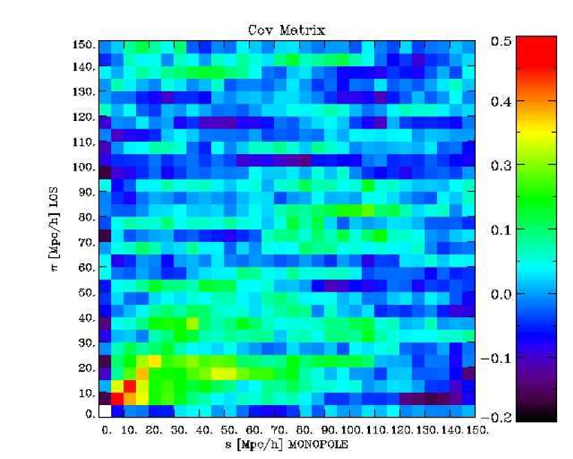
Because of the narrow range of $\sigma$ values ($0.5<\sigma<5.5\,h^{-1}\,{\rm Mpc}$) used in the radial measurement, the rBAO results are essentially independent from the monopole of the two-point function; fewer than 1% of the bins considered in the spherically averaged correlation function are used in the estimate of the radial correlation. For this reason we treat these two datasets as independent. We tested this explicitly using the mock LRG catalogues from Cabre & Gaztañaga (2009a) (the same set used to estimate the covarince matrix in the monopole), to evaluate the covariance of the radial and the monopole correlations. Fig. 2 shows the normalized covariance:

$$C_{ij}=\frac{1}{M}\sum_{k=1}^{M}\frac{[\xi_{\rm m}(i)^{k}-\widehat{\xi}_{\rm m}(i)]}{\sigma_{\rm m}(i)}\frac{[\xi_{\rm r}(j)^{k}-\widehat{\xi}_{\rm r}(j)]}{\sigma_{\rm r}(j)}$$ (2)

where $\xi_{\rm m}(i)^{k}$ and $\xi_{\rm r}(j)^{k}$ are the monopole and radial correlation in the $i$-th and $j$-th bins respectivelly measured in the $k$-th mock catalogue $(k=1,...M)$ and $\widehat{\xi}$ and $\sigma$ are the corresponding mean and rms fluctuations over the $M$ realizations. As shown in Fig.2 the covariance on the scales of interest in our analysis (larger than $40\,h^{-1}\,{\rm Mpc}$) is quite small (less than the noise in the estimation, of about 10%) which shows that the two datasets are indeed independent in practice. This implies that the rBAO measurements obtained from the radial correlation functions are independent from the monopole $\xi(s)$.

Figure 2: Normalized covariance matrix estimated from 216 mocks LRG samples. Here we test the covariance between the monopole correlation (horizontal axis) and the radial (LOS) correlation (vertical axis). The correlation is only important on small scales and is negligible (less than 10%) for the scales of interest here ($>40\,h^{-1}\,{\rm Mpc}$).

2.3 CMB data: temperature and polarization power spectra

The accuracy of recent observations of the CMB mean that this is the single most powerful dataset for constraining the values of cosmological parameters. The compilation of CMB measurements we use includes the temperature power spectrum in the range $2\leq\ell\leq 1000$ and the temperature-polarization power spectrum for $2\leq\ell\leq 450$ of the first five years of observations of the WMAP satellite (Hinshaw et al., 2009; Nolta et al., 2009); the bandpower temperature spectrum from the 2008 observations of the Arcminute Cosmology Bolometer Array Receiver (Kuo et al., 2007; Reichardt et al., 2009, ACBAR,) over the spherical harmonic range $910<\ell<1850$; temperature and polarization data from the Cosmic Background Imager (Readhead et al., 2004, CBI,) with $855<\ell<1700$; observations from the 2003 flight of BOOMERANG (Ruhl et al., 2003; Jones et  al., 2006; Montroy et al., 2006; Piacentini et al., 2006) in the range $925<\ell<1400$ and the recent results for the temperature and polarization power spectra measurements from QUaD (Ade et al., 2008) over the range $893<\ell<1864$. These measurements of the power spectrum of temperature fluctuations in the CMB cover the spherical harmonic range $2<\ell<1800$. Following Dunkley et al. (2009), in order to avoid cross-correlations with the WMAP data, we use only the bandpowers of the small scale CMB experiments that do not overlap with the signal-dominated WMAP data. Note that the QUaD measurements were not available at the time of the “WMAP+CMB” analysis carried out by Komatsu et al. (2008).

2.4 The Hubble diagram of type Ia supernovae

We also consider the constraints provided by the Hubble diagram of type Ia supernovae (SN) as provided by the UNION sample from (Kowalski et al., 2008). This compilation is drawn from 13 independent datasets processed using the SALT light curve fitter (Guy et al., 2005) and analysed in a uniform way. The sample contains a set of 57 low-redshift SN, the recent samples from the SuperNova Legacy Survey (Astier et al., 2006, SNLS,) and the Equation of State SupErNovae trace Cosmic Expansion (ESSENCE, Miknaitis et al., 2007), the high-redshift sample from the Hubble Space Telescope (Riess et al., 2004, 2007), as well older datasets (Riess et al., 1998; Perlmutter et al., 1999; Tonry et al., 2003; Barris et al., 2004). The final sample is the largest available to date, comprising 307 SN which pass the selection criteria.

Kowalski et al. (2008) suggest a way to include the effect of systematic errors when fitting the SN data. This estimation and those from other authors (Astier et al., 2006; Wood-Vasey et al., 2007; Hicken et al., 2009), predict different systematic errors in the estimated constraints on the dark energy equation of state, with values ranging from 5% to more than 10%. These approaches differ in the choice of which potential sources of systematic errors are taken into account and the estimation of their likely magnitude. It is our understanding that the community has not reached a consensus about the correct way to estimate the effect of the systematic errors in the analysis of the SN data. For this reason we follow other authors (e.g. Komatsu et al., 2009) and do not include the systematic errors in our constraints on cosmological parameters. However, the inclusion of the systematic errors in the SN data has important implications for the derived values of the dark energy equation of state (see Section 5.2). This should be borne in mind when comparing constraints obtained using SN data with those obtained using other datasets.

3 Methodology

In this section we summarize the approach used to obtain constraints on cosmological parameters. We start by describing he different parameter sets that we consider. The parametric model we use to describe the shape of the correlation function in redshift space is presented 3.2. The theoretical motivation for this parametric form can be found in Appendix A. In Section 3.2, we also compare the model with measurements made using numerical simulations. Section 3.3 describes the model we implement to describe the radial BAO measurements. The methodology we follow to explore and constrain the parameter spaces is discussed in Section 3.4.

3.1 The parameter space

In this paper we make the basic assumption that the primordial density fluctuations were adiabatic, Gaussian and had a power-law spectrum of Fourier amplitudes, with a negligible contribution from tensor modes. From the analysis of the fifth year of WMAP data, Komatsu et al. (2009) did not detect any deviation from these hypotheses at the 99% confidence limit (CL). Within this framework, a cosmological model can be defined by specifying the values of the following eight parameters:

$$\mathbf{P\equiv(}\Omega_{k},\omega_{\rm dm},\omega_{\rm b},\tau,n_{\rm s},A_{\rm s},\Theta,w_{\rm DE}).$$ (3)

We now go through the parameters in the above list, defining each one and also explaining how the values of other parameters are obtained, which we will refer to as derived parameters.

The homogeneous background cosmology is described through the various contributions to the mass-energy density. These are, in units of the critical density: $\Omega_{k}$, which describes the curvature of the universe; $\omega_{\rm dm}\equiv\Omega_{\rm dm}h^{2}$, the density of the dark matter (assumed cold, where $h$ is Hubble’s constant in units of $100\,{\rm kms}^{-1}{\rm Mpc}^{-1}$) and $\omega_{\rm b}\equiv\Omega_{\rm b}h^{2}$, the baryon density. We assume that massive neutrinos make no contribution to the mass budget. For most of this paper, we assume that the dark energy component has a constant equation of state independent of redshift, with the ratio of pressure to density given by $w_{\rm DE}$. In section 5.3 we relax this assumption and analyse models allowing for a time variation in this parameter. In this case we use the standard linear parametrization given by (Chevallier & Polarski, 2001; Linder et al., 2003)

$$w_{\rm DE}(a)=w_{\rm 0}+w_{a}(1-a),$$ (4)

where $a$ is the expansion factor and $w_{\rm 0}$ and $w_{a}$ are parameters.

The form of the initial fluctuations is described by two quantities; the scalar spectral index, $n_{\rm s}$ and the primordial amplitude of the scalar fluctuations $A_{\rm s}$. These parameter values are quoted at the “pivot” scale wavenumber of $k=0.05\,{\rm Mpc}^{-1}$.

We assume that the reionization of the neutral intergalactic medium occurred instantaneously, with an optical depth given by $\tau$. Finally, $\Theta$ gives the ratio of the sound horizon scale at the epoch of decoupling to the angular diameter distance to the corresponding redshift.

There are further basic quantities whose values can be derived from those listed in the set of Eq. (3):

$$\mathbf{P_{\rm derived}}\equiv(\Omega_{\rm m},h,\Omega_{\rm DE},\sigma_{8},z_{\rm re},t_{0}).$$ (5)

The matter density parameter is given by $\Omega_{\rm m}=\Omega_{\rm dm}+\Omega_{\rm b}$. The value of the Hubble constant is derived from $h=\sqrt{(\omega_{\rm dm}+\omega_{\rm b})/\Omega_{\rm m}}$. The energy-density of the dark energy is set by $\Omega_{\rm DE}=1-\Omega_{\rm m}-\Omega_{k}$. The results for $A_{\rm s}$ can be translated into a constraint on $\sigma_{8}$, the rms linear perturbation theory variance in spheres of radius $8~{}h^{-1}$Mpc, using the matter fluctuation transfer function. The redshift of reionization, $z_{\rm re}$, can be computed from the values of $\tau$, the Hubble constant and the matter and baryon densities (Tegmark et al., 1994). The age of the universe is $t_{0}$.

The $\Lambda$CDM cosmological model is the simplest model which can account for the wide variety of cosmological observations available today. This model is characterized by six parameters:

$$\mathbf{P^{6}_{\rm varied}}\equiv(\omega_{\rm dm},\omega_{\rm b},n_{\rm s},\tau,A_{\rm s},\Theta),$$ (6)

assuming $\Omega_{\rm k}=0$ and $w_{\rm DE}=-1$. This parameter space is well constrained by the temperature and polarization power spectrum measurements from five years of integration of the WMAP satellite (Komatsu et al., 2009). In Section 5.1 we analyse the impact of the measurement of the shape of $\xi(s)$ on the constraints in this parameter space.

Using the latest WMAP data, Komatsu et al. (2009) placed strong constraints on the possible deviations from the $\Lambda$CDM model, namely non-Gaussianity, the presence of isocurvature modes, deviations from a pure power law scalar primordial power spectrum, the presence of tensor modes, a non-negligible energy component in the form of massive neutrinos and parity-violation interactions. However, there are two parameters that signal important deviations of the standard $\Lambda$CDM model that can not be tightly constrained from CMB data alone: the curvature of the Universe $\Omega_{k}$ and the dark energy equation of state $w_{\rm DE}$. In order to assess the improvement on the constraints once the information on the shape of $\xi(s)$ is included in the analysis, we explore four parameter spaces which contain extensions of the simple $\Lambda$CDM set. First we extend the parameter set of Eq. (6) by adding a constant dark energy equation of state

$$\mathbf{P^{6+{\rm w_{DE}}}_{\rm varied}}\equiv(\omega_{\rm dm},\omega_{\rm b},n_{\rm s},\tau,A_{\rm s},\Theta,w_{\rm DE}),$$ (7)

fixing $\Omega_{k}=0$. The results obtained in this case are shown in Section 5.2.

In Section 5.3 we include the parametrization of Eq. (4) in our analysis and explore the extended parameter space

$$\mathbf{P^{6+{\rm w(a)}}_{\rm varied}}\equiv(\omega_{\rm dm},\omega_{\rm b},n_{\rm s},\tau,A_{\rm s},\Theta,w_{\rm 0},w_{a}),$$ (8)

where we also implement the hypothesis of a flat universe with $\Omega_{k}=0$. We also analyse the effect of dropping this assumption. First, in Section 5.4, we include $\Omega_{k}$ as a free parameter, with

$$\mathbf{P^{6+{\rm\Omega_{k}}}_{\rm varied}}\equiv(\omega_{\rm dm},\omega_{\rm b},n_{\rm s},\tau,A_{\rm s},\Theta,\Omega_{k}),$$ (9)

assuming that the dark energy is given by a cosmological constant (or vacuum energy) with $w_{\rm DE}=-1$. Finally, in Section 5.5, we also allow this parameter to vary freely and we explore the full parameter space of Eq. (3).

3.2 A physically motivated model for the correlation function

In the linear perturbation theory regime (valid when the fluctuation amplitude is small, for instance at high redshift or on very large scales), the shape of the matter correlation function is well understood and can be readily obtained using linear Boltzmann solvers, such as CAMB (Lewis et al., 2000). The shape of the correlation function, in the context of a standard adiabatic CDM model, is sensitive to the values of the matter density, $\Omega_{m}h^{2}$, the baryon density $\Omega_{b}h^{2}$, the spectral tilt $n_{\rm s}$ and the density parameter of massive neutrinos. The evolution with redshift of the correlation function is well understood in the linear regime. In this case, each Fourier mode of the density field evolves independently of the others and the shape of $\xi$ is unaltered, although the overall amplitude changes with time.

Unfortunately this simple behaviour is modified by a number of nonlinear phenomena, which affect different scales at different epochs. These include nonlinear effects generated by the latter stages of gravitational instability, redshift-space distortions caused by gravitationally induced motions and a possible non-trivial scale dependent bias relation between the distribution of galaxies and the underlying dark matter field (see, for example, the step-by-step illustration of these effects given by Angulo et al., 2008). Nonlinear growth results in cross-talk between different Fourier modes and introduces scale dependent patterns in the clustering, even on large scales. This is particularly noticeable in the appearance of the BAO bump, which is sensitive to the match between the amplitude and phases of the fluctuations around the peak scale. Due to the distortion of the Fourier modes from their original values, nonlinear growth causes the BAO bump to become smeared out and also to lose contrast. Such effects cannot be ignored when modelling low-redshift data.

Figure 3: The correlation function of dark matter halos in redshift space measured in an ensemble of 50 large-volume N-body simulations (with total volume of $\sim 105\,h^{-3}\,{\rm Gpc}^{3}$). The error bars correspond to the error on the mean of the ensemble and are obtained from the scatter among the $50$ realizations. The best fitting parametric model used in this work, Eq. (10), is shown by the solid blue line (note the fit takes into account the covariance between the bins). The dashed line corresponds to setting $A_{\rm MC}=0$ and highlights the importance of this term in matching the shape of the correlation function at $r<80\,h^{-1}\,{\rm Mpc}$. The scaling uses $r_{\rm BAO}=102h^{-1}$Mpc.

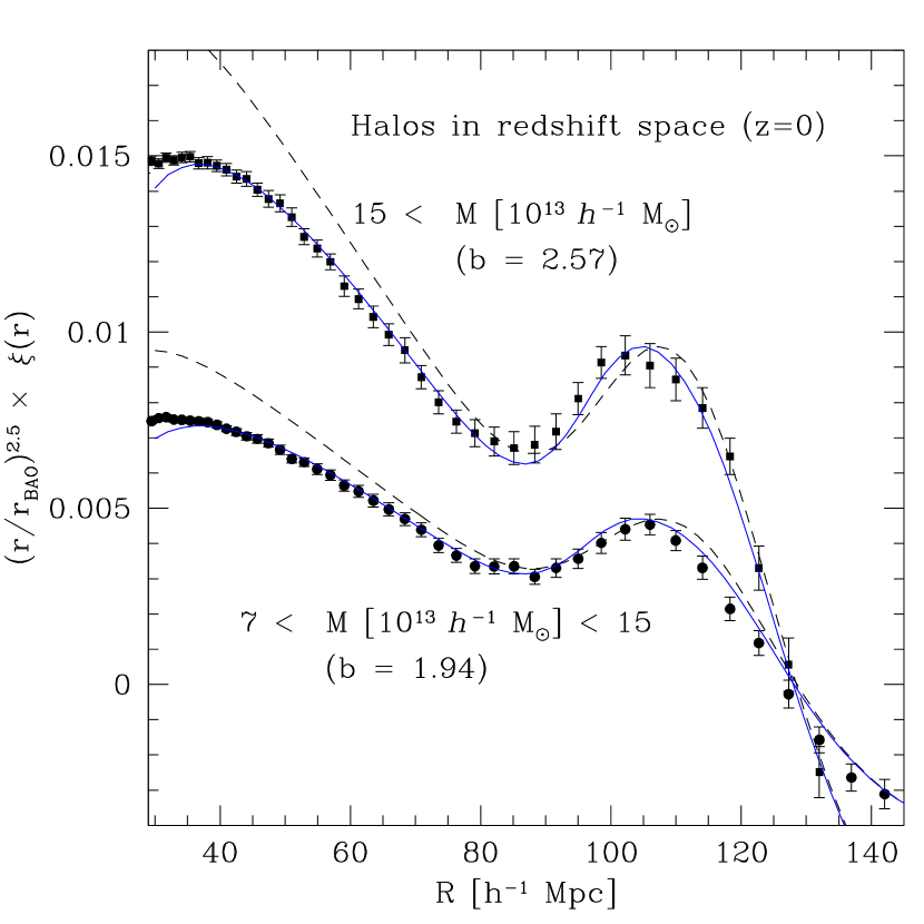
On large scales, ($r>30\,h^{-1}\,{\rm Mpc}$), the correlation function falls sharply with increasing comoving pair separation, scaling roughly as a power law $\sim r^{-\gamma}$, with $\gamma\sim 2.5$. At even larger separations, this behaviour is altered by the emergence of a bump known as the BAO peak (e.g. see Fig. 3). This feature, first measured for LRGs by Eisenstein et al. (2005), is centered at about $110\,h^{-1}\,{\rm Mpc}$ and has a width of $\sim 20\,h^{-1}\,{\rm Mpc}$. The amplitude of the peak in the LRG correlation function corresponds to a $\sim 1\%$ excess in the number of LRG pairs above the number expected in a random distribution (e.g. Cabre & Gaztañaga, 2009a).

To model the shape of the correlation function on large scales, we follow Crocce & Scoccimarro (2008) and Sánchez et al. (2008) and adopt the following parametrization:

$$\xi_{\rm NL}(r)=b^{2}\{\xi_{\rm L}(r)\otimes{\rm e}^{-(k_{\star}r)^{2}}+A_{\rm MC}\,\xi^{\prime}_{\rm L}(r)\,\xi^{(1)}_{\rm L}(r)\},$$ (10)

where $b$, $k_{\star}$ and $A_{\rm MC}$ are nuisance parameters, and the symbol $\otimes$ denotes a convolution. Here $\xi^{\prime}_{\rm L}$ is the derivative of the linear correlation function and $\xi^{(1)}_{\rm L}(r)$ is defined by the integral:

$$\xi_{\rm L}^{(1)}(r)\equiv\hat{r}\cdot\nabla^{-1}\xi_{\rm L}(r)=4\pi\,\int P_{\rm L}(k)\,j_{1}(kr)k\,{\rm d}k,$$ (11)

with $j_{\rm 1}(y)$ denoting the spherical Bessel function of order one. The model in Eq. 10 is primarily motivated by RPT, where the matter power spectrum is written as $P=G^{2}P_{L}+P_{MC}$, with $G$ a nonlinear growth factor and $P_{\rm MC}$ being the power generated by mode-coupling. To a very good approximation $G$ is of Gaussian form, while at large scales the leading order contribution of $P_{\rm MC}$ in real space is $\sim\xi^{(1)}_{L}\xi^{\prime}_{L}$ (see Appendix A for a detailed discussion). The Gaussian degradation of the BAO information was also shown to be a good description by Eisenstein et al. (2006).

We now demonstrate how accurately the model of Eq. (10) can reproduce the spatial clustering of halo samples with comoving number densities similar to that of the LRGs in DR6. To this end we utilize an ensemble of $50$ realizations of collisionless dark matter N-body simulations. Each simulation contains $640^{3}$ particles in a comoving volume $V=L^{3}=(1280\,h^{-1}\,{\rm Mpc})^{3}$. The cosmological parameters were set to $\Omega_{m}=0.27$, $\Omega_{\Lambda}=0.7$, $\Omega_{b}=0.046$ and $h=0.72$. The initial power spectrum had spectral index $n_{s}=1$ and was normalized to give $\sigma_{8}=0.9$ when linearly extrapolated to $z=0$. Halos were identified using the friends-of-friends algorithm with linking-length parameter $l=0.2$ (see Smith et al., 2008; Crocce & Scoccimarro, 2008, for more details).

Fig. 3 shows the 2-point correlation function measured in redshift-space at $z=0$ for two non-overlapping samples of dark matter haloes of masses $7\times 10^{13}<M[{\it h}^{-1}\,{\rm M}_{\odot}]<15\times 10^{13}$ and $15\times 10^{13}<M[{\it h}^{-1}\,{\rm M}_{\odot}]$ (with number densities $\bar{n}[{\it h}^{3}\,{\rm Mpc}^{-3}]=1.88\times 10^{-5}$ and $3.46\times 10^{-5}$ respectively). Our redshift space measurements were done considering the contribution of peculiar velocities along one dimension in the simulation (i.e. recreating a plane-parallel configuration).

Szapudi (2004) discussed in depth the issue of wide angle redshift space distortions. He found that opening angles $\theta\lesssim 15^{\circ}-20^{\circ}$ would ensure the validity of the plane-parallel approximation. For the redshift range of the LRG sample considered in our analysis ($0.15<z<0.47$) and the largest pair-distance separation allowed ($s_{\rm max}=150\,h^{-1}{\rm Mpc}$), the maximum opening angle is given by $\sin(\theta_{\rm max})=s_{\rm max}/D_{\rm A}(z=0.15)$, which implies $\theta_{\rm max}\approx 20^{\circ}$. For the mean redshift of the sample the angle subtended by $s_{\rm max}$ is $\theta\approx 10^{\circ}$, well within the validity of the plane-parallel approximation.

The error bars plotted show the error on the mean obtained from the ensemble of 50 simulations. Each simulation has a larger volume than the LRG sample we use from DR6. Therefore these errors are $\approx\sqrt{2}\times\sqrt{50}=10$ times smaller than they would be for the LRG sample. This means that the deviations between models (solid lines) and simulation results (points) are not important for our purposes.

The parametrization given in Eq. (10) corresponds to the solid blue line in Fig. 3. The corresponding best-fit $\chi^{2}$ values for the nuisance parameters $(k_{\star}[{\it h}\,{\rm Mpc}^{-1}],b,A_{\rm MC})$ were $(0.142,1.94,3.23)$ and $(0.146,2.75,4.53)$ respectively. Clearly, the model can accurately describe the clustering of halos in redshift space.

Sánchez et al. (2008) also compared Eq. (10) against measurements of the non-linear correlation function from a similar large ensemble of N-body simulations at various redshifts, and confirmed that this form gives an essentially unbiased measurement of the dark energy equation of state using both, real and redshift space information.

The dashed line in Fig. 3 corresponds to Eq. (10) with $A_{\rm MC}=0$. From the plot we can see that the inclusion of this term is the key to recovering the correct clustering shape at separations smaller than the BAO bump. In addition it contributes slightly to the shape of the bump and alleviates a systematic effect related to the position of the BAO peak (Crocce & Scoccimarro, 2008) (but this is sub-dominant for the survey volume being considered). In subsequent sections we check that this nuisance parameter is not degenerate with any of the cosmological parameters.

On theoretical grounds, one expects the smoothing length $k_{\star}^{-1}$ to depend on cosmology (i.e. aside from galaxy type or redshift) with, for example, a $10\%$ increase in $\Omega_{\rm m}$ expected to increase $k_{\star}$ by about $4\%$ (Crocce & Scoccimarro, 2006b; Matsubara, 2008). In view of this, we decided to consider $k_{\star}$ as a nuisance parameter at the expense of a possible increase in error bars. Note that this is at variance with the approach of Eisenstein et al. (2005), Tegmark et al. (2006) and Percival et al. (2007c) who kept this length fixed.

In summary, for each cosmological model we compute the linear correlation function $\xi_{\rm L}(r)$ using CAMB to generate the corresponding transfer function, and simulate nonlinear effects through Eq. (10) after computing $\xi_{\rm L}^{\prime}(r)$ and $\xi_{\rm L}^{(1)}(r)$ from Eq. (11).

3.3 A model for the radial acoustic scale

Here we describe the simple model that we use to compute the dimensionless redshift radial acoustic scale $\Delta z_{\rm BAO}$ for a given choice of the cosmological parameters of Eq. (3).

The value of $\Delta z_{\rm BAO}$ can be computed as,

$$\Delta z_{\rm BAO}(z)=\frac{H(z)r_{\rm s}(z_{\rm d})}{c},$$ (12)

where $H(z)$ is the Hubble constant at the mean redshift of the measurements ($z_{\rm m}=0.24$ and 0.43), and $r_{\rm s}(z_{\rm d})$ is the comoving sound horizon at the drag epoch, which is given by

$$r_{\rm s}(z)=\frac{c}{\sqrt{3}}\int_{0}^{(1+z)^{-1}}\frac{{\rm d}a}{a^{2}H(a)\sqrt{1+Ra}},$$ (13)

where $R=3\Omega_{\rm b}/4\Omega_{\rm\gamma}$ and $\Omega_{\rm\gamma}=2.469\times 10^{-5}\,h^{-2}$ for a CMB temperature $T_{\rm CMB}=2.725\,{\rm K}$. The value of $z_{\rm d}$ can be computed with high accuracy from the values of $\omega_{\rm b}$ and $\omega_{\rm dm}$ using the fitting formulae of Eisenstein & Hu (1998).

The radial BAO scale measurements can be used to place constraints on cosmological parameters independently of other datasets. Being a purely geometrical test, as in the case of the SN data, the radial BAO measurements are not sensitive to all the cosmological parameters of Eq. (3) since they contain no information about the primordial spectrum of density fluctuations, that is $A_{\rm s}$ and $n_{\rm s}$, and of the optical depth to the last scattering surface $\tau$.

Table 1: The parameter space probed in our analysis. We assume a flat prior in each case. The parameter spaces that we consider are set out in Section 3.1.

Parameter	Allowed range
$\omega_{\rm dm}$	0.01 – 0.99
$\omega_{\rm b}$	0.005 – 0.1
$\Theta$	0.5 – 10
$\tau$	0 – 0.8
$n_{\rm s}$	0.5 – 1.5
$\ln(10^{10}A_{\rm s})$	2.7 – 4.0
$w_{\rm DE}$	$-$2. – 0
$\Omega_{k}$	$-$0.3 – 0.3

3.4 Practical issues when constraining parameters

We use a Bayesian approach and explore the different parameter spaces defined in Section 3.1 using the Markov Chain Monte Carlo (MCMC) technique. Our results were generated with the publicly available CosmoMC code of Lewis & Bridle (2002). CosmoMC uses the camb package to compute power spectra for the CMB and matter fluctuations (Lewis, Challinor & Lasenby 2000). We use a generalized version of camb which supports a time-dependent dark energy equation of state (Fang et al., 2008). For each parameter set considered, we ran twelve separate chains which were stopped when the Gelman and Rubin (1992) criteria reached $R<1.02$. We implemented flat priors on our base parameters. Table 1 summarizes the ranges considered for different cosmological parameters in the cases where their values are allowed to vary.

In order to establish the link between a given cosmological model and the datasets described in Section 2 it is necessary to include a small set of extra parameters given by

$$\mathbf{P_{\rm extra}}\equiv(b,k_{\star},A_{\rm MC},A_{\rm SZ}),$$ (14)

to the parameter sets described in Section 3.1. The bias factor $b$, describes the difference in amplitude between the galaxy correlation function and that of the underlying dark matter. The values of $k_{\star}$ and $A_{\rm MC}$ from Eq. (10) are also included as free parameters in our parameter space. $A_{\rm SZ}$ gives the amplitude of the contribution from the Sunyaev-Zeldovich effect to the CMB angular power spectrum on small scales (high $\ell$). When quoting constraints on the parameters of Eq. (3) and (5), the values of these extra parameters are marginalized over. In the case of $b$, this is done using the analytic expression given in Appendix F of Lewis & Bridle (2002), but the remaining parameters are included in our Monte Carlo analysis (see Section 3.4).

There is one important point that must be considered in order to make a comparison between the model of Eq.(10) and the observational data of the LRG redshift-space correlation function. When measuring $\xi(s)$, in order to map the observed galaxy redshifts and angular positions on the sky into distances, it is necessary to assume a fiducial cosmological model. This choice has an impact on the results obtained.

Figure 4: The impact of a mismatch in cosmology on the form of the correlation function. The upper panel shows the difference between the correlation functions measured assuming different fiducial cosmologies ($\Lambda$CDM models with varying $\Omega_{\rm m}$) from that obtained assuming $\Omega_{\rm m}=0.25$. The lower panel shows the same comparison after applying the scale shift of Eq. (15) to take into account the change in the value of $\Omega_{\rm m}$.

One possible way to deal with this is to re-compute the correlation function and its covariance matrix for the cosmology corresponding to each point in the Markov chains, and then use this measurement when computing the likelihood of the given cosmological model. This approach is infeasible since it would require an exceedingly large amount of computing time. Instead we follow an alternative approach by indirectly including the effect of the choice of the cosmology on the model correlation function. To do this we follow Eisenstein et al. (2005) and simply rescale the distances in the model correlation function by a factor

$$\alpha=\frac{D_{{\rm V}}^{\rm model}}{D_{\rm V}^{{\rm fiducial}}},$$ (15)

where the effective distance $D_{{\rm V}}(z_{\rm m})$ to the mean redshift of the survey $z_{\rm m}=0.35$, is computed for each model as

$$D_{\rm V}(z_{\rm m})=\left[D_{\rm A}^{2}(z_{\rm m})\frac{cz}{H(z_{\rm m})}\right]^{1/3}.$$ (16)

where $D_{\rm A}(z)$ is the comoving angular diameter distance given by

$$D_{\rm A}(z)=\frac{c}{H_{0}\sqrt{|\Omega_{k}}|}f_{k}\left(H_{0}\sqrt{|\Omega_{k}|}\int_{0}^{z}\frac{{\rm d}z^{\prime}}{H(z^{\prime})}\right),$$ (17)

where

$$f_{k}(x)=\cases{{\rm sinh}(x)&if$(\Omega_{k}>0)$,\cr x&if$(\Omega_{k}=0)$,\cr\sin(x)&if$(\Omega_{k}<0)$.\cr}$$ (18)

The exponents within the square bracket on the right-hand side of Eq. (16) assume that the survey covers a wide solid angle, rather than a pencil-beam.

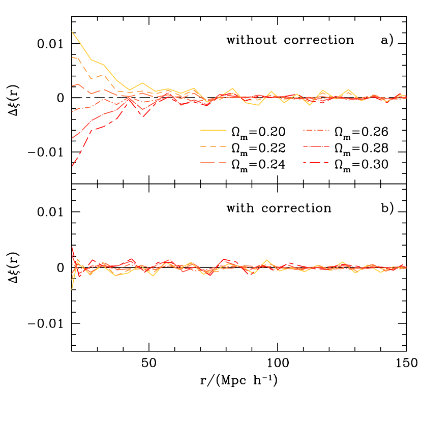
We can test the effectiveness of the correction factor given by Eq. (15) by applying it to different estimates of the correlation function computed with varying choices of the fiducial cosmology. Cabre & Gaztañaga (2009a) computed the redshift space correlation function of SDSS-DR6 LRGs assuming different flat fiducial cosmologies with values of $\Omega_{m}$ ranging from 0.2 to 0.3. The upper panel of Fig. 4 shows the difference of these estimates from the one obtained for $\Omega_{\rm m}=0.25$. It is clear that the choice of the cosmological model affects the shape of the correlation function. The effect of this choice is particularly important on small scales ($r<70\,h^{-1}\,{\rm Mpc}$), but also introduces a small distortion to the shape of the acoustic peak, shifting its position towards larger (smaller) scales for smaller (larger) values of $\Omega_{\rm m}$. If unaccounted for, this difference would bias the constraints obtained on the cosmological parameters. The lower panel shows the same quantity once the correction factor of Eq. (15) has been applied. Clearly, this simple correction is able to account for the choice of the fiducial cosmological model. We use this correction factor to translate the model correlation function to the fiducial cosmology used by Cabre & Gaztañaga (2009a) to estimate the LRG $\xi(s)$ (a flat $\Lambda$CDM mode with $\Omega_{\rm m}=0.25$). We then compute the likelihood of the model assuming the Gaussian form ${\cal L}\propto\exp(-\chi^{2}/2)$.

4 Testing the model of $\xi(s)$

In this section we analyse the sensitivity of the parameter constraints to the details of the procedure we follow to compute the likelihood of a given model. For the purpose of this exercise we use the information contained in the correlation function of LRGs combined with the latest results from the WMAP satellite alone to constrain the parameter set of Eq. (7), and assess the impact on the results of varying choices in our analysis procedure.

Figure 5: The dependence of the constraints on cosmological parameters on the minimum pair separation, $r_{\rm min}$, included in the correlation function measurement. The points show the mean value of the likelihood for each parameter and the error bars show the 68% CL.

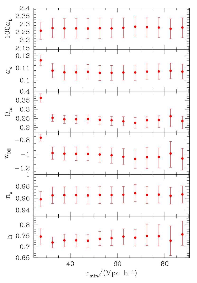
First we study the sensitivity of the results to the range of scales in $\xi(s)$ included in the analysis. Sánchez et al. (2008) showed that the model of Eq. (10) gives an accurate description of the redshift-space halo correlation function measured from N-body simulations on scales in the range $60\,h^{-1}\,{\rm Mpc}\leq r\leq 180\,h^{-1}{\rm Mpc}$. In Section 3.2, we showed that the second term in Eq. (10) also helps to reproduce the results from N-body simulations down to scales of $40\,h^{-1}{\rm Mpc}$. Even though our measurement of $\xi(s)$ extends to larger scales, the measurement beyond $150\,h^{-1}\,{\rm Mpc}$ is noisy and does not have any effect on the constraints. Besides, Cabre & Gaztañaga (2009a) showed that on these large scales, the measurement of the redshift space correlation function exhibits an excess in the amplitude with respect to the previous estimate of Eisenstein et al. (2005). For this reason we have chosen to set a maximum distance $r_{\rm max}=150\,h^{-1}\,{\rm Mpc}$ in all subsequent analyses.

Table 2: The marginalized 68% interval constraints on the cosmological parameters of the $\Lambda$CDM model obtained using different combinations of the datasets described in Section 2, as stated in the column headings.

	CMB	CMB + $\xi(s)$	CMB + rBAO	CMB + SN	CMB + $\xi(s)$	CMB + $\xi(s)$	$\xi(s)$+ rBAO
					+ rBAO	+ rBAO + SN
$100\Theta$	$1.0416_{-0.0023}^{+0.0023}$	$1.0415_{-0.0022}^{+0.0022}$	$1.0413_{-0.0022}^{+0.0022}$	$1.0413_{-0.0022}^{+0.0022}$	$1.0414_{-0.0022}^{+0.0022}$	$1.0412_{-0.0022}^{+0.0022}$	$0.987_{-0.069}^{+0.065}$
$\omega_{\rm dm}$	$0.1091_{-0.0053}^{+0.0053}$	$0.1076_{-0.0038}^{+0.0038}$	$0.1108_{-0.0036}^{+0.0036}$	$0.1125_{-0.0038}^{+0.0038}$	$0.1095_{-0.0032}^{+0.0032}$	$0.1110_{-0.0029}^{+0.0029}$	$0.091_{-0.038}^{+0.040}$
$100\,\omega_{\rm b}$	$2.282_{-0.051}^{+0.050}$	$2.280_{-0.051}^{+0.050}$	$2.277_{-0.050}^{+0.051}$	$2.270_{-0.051}^{+0.051}$	$2.276_{-0.049}^{+0.049}$	$2.267_{-0.051}^{+0.050}$	$3.0_{-1.7}^{+2.0}$
$\tau$	$0.088_{-0.016}^{+0.016}$	$0.090_{-0.017}^{+0.017}$	$0.088_{-0.016}^{+0.016}$	$0.087_{-0.016}^{+0.016}$	$0.088_{-0.016}^{+0.016}$	$0.086_{-0.016}^{+0.016}$	-
$n_{\rm s}$	$0.965_{-0.013}^{+0.013}$	$0.965_{-0.012}^{+0.012}$	$0.962_{-0.012}^{+0.012}$	$0.960_{-0.012}^{+0.012}$	$0.963_{-0.011}^{+0.011}$	$0.960_{-0.011}^{+0.011}$	$1.06_{-0.31}^{+0.34}$
$\ln(10^{10}A_{\rm s})$	$3.066_{-0.037}^{+0.037}$	$3.059_{-0.038}^{+0.038}$	$3.067_{-0.036}^{+0.036}$	$3.070_{-0.036}^{+0.036}$	$3.062_{-0.036}^{+0.036}$	$3.065_{-0.036}^{+0.036}$	-
$\Omega_{\rm DE}$	$0.749_{-0.026}^{+0.026}$	$0.755_{-0.018}^{+0.018}$	$0.740_{-0.017}^{+0.017}$	$0.730_{-0.020}^{+0.019}$	$0.747_{-0.014}^{+0.014}$	$0.739_{-0.013}^{+0.013}$	$0.782_{-0.041}^{+0.040}$
$\Omega_{\rm m}$	$0.251_{-0.026}^{+0.026}$	$0.244_{-0.018}^{+0.018}$	$0.260_{-0.017}^{+0.017}$	$0.270_{-0.019}^{+0.020}$	$0.253_{-0.014}^{+0.014}$	$0.261_{-0.013}^{+0.013}$	$0.218_{-0.040}^{+0.041}$
$\sigma_{8}$	$0.795_{-0.029}^{+0.028}$	$0.787_{-0.024}^{+0.024}$	$0.802_{-0.024}^{+0.024}$	$0.810_{-0.023}^{+0.023}$	$0.795_{-0.022}^{+0.021}$	$0.802_{-0.021}^{+0.021}$	-
$t_{0}/{\rm Gyr}$	$13.64_{-0.11}^{+0.11}$	$13.64_{-0.10}^{+0.10}$	$13.668_{-0.097}^{+0.099}$	$13.69_{-0.10}^{+0.10}$	$13.660_{-0.096}^{+0.097}$	$13.682_{-0.094}^{+0.095}$	$14.4_{-2.9}^{+3.2}$
$z_{\rm re}$	$10.5_{-1.3}^{+1.3}$	$10.5_{-1.3}^{+1.3}$	$10.4_{-1.3}^{+1.4}$	$10.4_{-1.3}^{+1.3}$	$10.4_{-1.3}^{+1.3}$	$10.4_{-1.3}^{+1.3}$	-
$h$	$0.726_{-0.024}^{+0.025}$	$0.731_{-0.018}^{+0.018}$	$0.718_{-0.016}^{+0.016}$	$0.710_{-0.018}^{+0.017}$	$0.723_{-0.013}^{+0.013}$	$0.716_{-0.012}^{+0.012}$	$0.73_{-0.14}^{+0.15}$

Fig. 5 shows the one-dimensional marginalized constraints on a subset of the parameters space of Eq. (7) as a function of the minimum scale, $r_{\rm min}$, included in the analysis. For $r_{\rm min}<40\,h^{-1}\,{\rm Mpc}$ we see that the constraints start to vary with $r_{\rm min}$. Coincidentally, in this regime the model of Eq. (10) starts to deviate from the N-body measurements of the correlation function discussed in Sec. 3.2. On such scales, extra terms beyond the one-loop contribution $\sim\xi^{\prime}$ to $\xi_{\rm MC}$ are expected to become important, which implies the breakdown of our ansatz.

For $r_{\rm min}>40\,h^{-1}\,{\rm Mpc}$, Fig. 5 shows that the constraints on the values of the cosmological parameters are very stable. Furthermore, the mean values obtained for these parameters using CMB data plus the LRG correlation function are in complete agreement with the ones obtained from CMB information only. The allowed regions of some parameters, like $\omega_{\rm b}$ or $n_{\rm s}$ which are tightly constrained by the CMB data alone show almost no change on varying $r_{\rm min}$. Other parameters, such as $\Omega_{\rm m}$ or $w_{\rm DE}$ show a substantial increase in their allowed regions as the data from small scales is gradually excluded from the analysis. For $r_{\rm min}=42.5\,h^{-1}\,{\rm Mpc}$ we obtain a constraint on the dark energy equation of state of $w_{\rm DE}=-0.996_{-0.095}^{+0.097}$, while for $r_{\rm min}=82.5\,h^{-1}\,{\rm Mpc}$, that is including only scales close to the acoustic peak in $\xi(s)$, we get $w_{\rm DE}=-0.99_{-0.19}^{+0.17}$. This approximately factor of two change in the error bar highlights the importance of the inclusion of information from the shape of $\xi(s)$ on intermediate scales. Based on this comparison and the results of Section 3.2, we have chosen to set $r_{\rm min}=42.5\,h^{-1}\,{\rm Mpc}$ in the subsequent analysis.

We also studied the impact of the correction to the measured correlation function to take into account changing the fiducial cosmology assumed when estimating $\xi(s)$. For this test we obtained constraints in the same parameter space without applying the correction of Eq. (15). The results obtained in this way are entirely consistent with those obtained when this correction is applied. The mean values of all the parameters remain practically identical with the exception of $\Omega_{\rm m}$ which shows a slight shift towards higher values of approximately 0.2$\sigma$. The allowed regions for these parameters also show almost no variation with a slight increase in the confidence limits of $\Omega_{\rm m}$ and $w_{\rm DE}$ of approximately 0.3$\sigma$. A similar shift but towards smaller values of $\Omega_{\rm m}$ is obtained on setting $A_{\rm MC}=0$ in the second term of the right hand side of Eq. (10). This is in agreement with the results of Sánchez et al. (2008), who found that the two most important parameters of this parametrization required to obtain a good description of the shape of the two-point correlation function are $k_{\star}$ and $b$ (which in this case is marginalized over).

Figure 6: The marginalized, one-dimensional posterior likelihood in the $\Lambda$CDM parameter space (Eq. 6) obtained from CMB information only (dashed lines), CMB plus the shape of $\xi(s)$ (solid line) and the full constraints including also rBAO and SN data (dot-dashed lines).

In Section 5 we also present constraints obtained from the combination of the two large scale structure datasets we use in our analysis, the LRG $\xi(s)$ and the position of the radial acoustic peak, without including any CMB information. The fact that the correction for the fiducial cosmology does not significantly change the obtained results when the LRG $\xi(s)$ is used in combination with the CMB, is not due to the later keeping the constraints sufficiently close to the fiducial cosmology. As we will see later (see Section 5.2) the constraints in this parameter space from CMB data alone present a strong degeneracy between $\Omega_{\rm m}$ and $w_{\rm DE}$, allowing for models that differ substantially from our fiducial cosmology of $\Omega_{\rm m}=0.25$ and $w_{\rm DE}=-1$. Nonetheless, these models are ruled out by the $\xi(s)$ data itself, (which on large scales is insensitive to this correction), since the position of the acoustic peak shows a strong variation in these models. The only region of the parameter space allowed by the data is that where the effect of the correction of Eq. (15) is small (although not completely negligible). This is the reason why the obtained constrains are not extremely sensitive to this correction. This also implies that this correction should not be too important even in the case in which the LRG $\xi(s)$ is combined with the radial acoustic peak whitout including any CMB data. We have tested this explicitly and found that the resulting mean values of the cosmological parameters obtained for this dataset combination when this correction is not applied show no variation with respect to the ones obtained when it is used. The only effect of ignoring this correction is a small artificial increase of the allowed regions of $\Omega_{\rm m}$ and $w_{\rm DE}$ of the same order as in the previous case. Setting $A_{\rm MC}=0$ for this combination of datasets also produces a small shift towards smaller values of $\Omega_{\rm m}$, which in this case is much smaller than the allowed region for this parameter. These tests show that our constraints are robust with respect to the details of our analysis technique.

5 Constraints on cosmological parameters

In this section, we carry out a systematic study of the constraints placed on the values of the cosmological parameters for the different parameter spaces defined in Section 3.4. In Section 5.1, we present the results for the simple $\Lambda$CDM cosmological model with six free parameters. In Section 5.2, we consider an extension to this parameter set, allowing the dark energy equation of state $w_{\rm DE}$ to float (but without any redshift dependence). Section 5.3 gives the constraints on models where the time variation of $w_{\rm DE}$ is parametrized according to Eq. (4). In Section 5.4 we discuss our constraints on non-flat models, analysing the parameter space of Eq. (9). Finally, Section 5.5 shows the constraints on the full parameter space of Eq. (3), allowing both for non-flat models and more general dark energy models. Tables 2-6 compare the constraints obtained in these parameter spaces using different combinations of the datasets described in Section 2.

5.1 The basic $\Lambda$CDM model

Due to the successful reproduction of a wide variety of observations, the $\Lambda$CDM model has emerged over the past decade as the new standard cosmological model. The recent results from five years of observations by the WMAP satellite have helped to reinforce this conclusion. The latest WMAP data give a much better estimation of the third acoustic peak in the CMB temperature power spectrum, as well as the low-$\ell$ polarization signal. Thanks to these improvements, the WMAP data alone has been able to provide much tighter constraints on this basic cosmological model than was possible when using earlier releases.

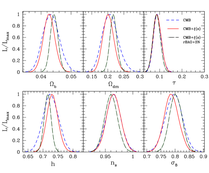
Table 2 summarizes the constraints on the parameters of this simple model for different combinations of datasets. Fig. 6 shows the marginalized likelihoods for this parameter set obtained using CMB data alone (dashed lines), CMB plus the LRG $\xi(s)$ (solid lines) and the full combination of the datasets described in Section 2 i.e. CMB+ LRG $\xi(s)$+rBAO+SN (dot-dashed line). Several parameters, such as $\omega_{\rm b}$, $\omega_{\rm c}$ and $\tau$, are tightly constrained by the CMB data alone, and show almost no variation when other datasets are included in the analysis. On the other hand, the constraints on the parameters of the energy budget do show a marked improvement on adding further datasets.

Table 3: The marginalized 68% interval constraints on cosmological parameters allowing for variations in the (redshift independent) dark energy equation of state (i.e. the parameter set defined by Eq.(7)), obtained using different combinations of the datasets described in Section 2, as stated in the column headings.

	CMB	CMB + $\xi(s)$	CMB + rBAO	CMB + SN	CMB + $\xi(s)$	CMB + $\xi(s)$	$\xi(s)$+ rBAO
					+ rBAO	+ rBAO + SN
$w_{\rm DE}$	$-0.73_{-0.30}^{+0.30}$	$-0.988_{-0.088}^{+0.088}$	$-0.92_{-0.15}^{+0.15}$	$-0.950_{-0.055}^{+0.054}$	$-0.999_{-0.091}^{+0.090}$	$-0.969_{-0.052}^{+0.052}$	$-1.05_{-0.15}^{+0.16}$
$100\Theta$	$10413_{-0.0024}^{+0.0023}$	$1.0415_{-0.0023}^{+0.0023}$	$1.0414_{-0.0022}^{+0.0022}$	$1.0413_{-0.0022}^{+0.0023}$	$1.0413_{-0.0023}^{+0.0023}$	$1.0414_{-0.0022}^{+0.0022}$	$0.994_{-0.075}^{+0.071}$
$\omega_{\rm dm}$	$0.1105_{-0.0050}^{+0.0052}$	$0.1068_{-0.0048}^{+0.0049}$	$0.1095_{-0.0045}^{+0.0045}$	$0.10933_{-0.0050}^{+0.0049}$	$0.1092_{-0.0042}^{+0.0042}$	$0.1088_{-0.0041}^{+0.0040}$	$0.099_{-0.045}^{+0.049}$
100 $\omega_{\rm b}$	$2.266_{-0.052}^{+0.053}$	$2.280_{-0.052}^{+0.052}$	$2.277_{-0.051}^{+0.051}$	$2.272_{-0.052}^{+0.052}$	$2.275_{-0.049}^{+0.00051}$	$2.275_{-0.050}^{+0.051}$	$3.0_{-1.7}^{+1.8}$
$\tau$	$0.089_{-0.017}^{+0.017}$	$0.090_{-0.017}^{+0.017}$	$0.090_{-0.017}^{+0.017}$	$0.089_{-0.017}^{+0.017}$	$0.088_{-0.017}^{+0.017}$	$0.088_{-0.016}^{+0.016}$	-
$n_{\rm s}$	$0.959_{-0.014}^{+0.014}$	$0.965_{-0.013}^{+0.012}$	$0.963_{-0.012}^{+0.012}$	$0.961_{-0.013}^{+0.013}$	$0.963_{-0.012}^{+0.011}$	$0.963_{-0.012}^{+0.012}$	$1.03_{-0.32}^{+0.37}$
$\ln(10^{10}A_{\rm s})$	$3.067_{-0.037}^{+0.038}$	$3.057_{-0.037}^{+0.037}$	$3.066_{-0.037}^{+0.037}$	$3.064_{-0.037}^{+0.038}$	$3.062_{-0.036}^{+0.035}$	$3.060_{-0.036}^{+0.036}$	-
$\Omega_{\rm DE}$	$0.63_{-0.12}^{+0.12}$	$0.754_{-0.021}^{+0.020}$	$0.723_{-0.034}^{+0.034}$	$0.733_{-0.019}^{+0.018}$	$0.746_{-0.017}^{+0.017}$	$0.739_{-0.013}^{+0.013}$	$0.778_{-0.045}^{+0.045}$
$\Omega_{\rm m}$	$0.36_{-0.12}^{+0.12}$	$0.245_{-0.020}^{+0.021}$	$0.277_{-0.034}^{+0.034}$	$0.267_{-0.018}^{+0.019}$	$0.254_{-0.017}^{+0.017}$	$0.261_{-0.013}^{+0.013}$	$0.222_{-0.045}^{+0.045}$
$\sigma_{8}$	$0.724_{-0.085}^{+0.087}$	$0.778_{-0.045}^{+0.045}$	$0.774_{-0.060}^{+0.060}$	$0.780_{-0.037}^{+0.038}$	$0.793_{-0.045}^{+0.043}$	$0.781_{-0.034}^{+0.035}$
$t_{0}/{\rm Gyr}$	$14.01_{-0.38}^{+0.40}$	$13.65_{-0.11}^{+0.11}$	$13.74_{-0.14}^{+0.14}$	$13.71_{-0.10}^{+0.10}$	$13.67_{-0.10}^{+0.10}$	$13.689_{-0.095}^{+0.095}$	$14.3_{-3.0}^{+3.1}$
$z_{\rm re}$	$10.7_{-1.4}^{+1.4}$	$10.5_{-1.3}^{+1.3}$	$10.6_{-1.3}^{+1.4}$	$10.5_{-1.3}^{+1.3}$	$10.4_{-1.4}^{+1.4}$	$10.4_{-1.3}^{+1.3}$	-
$h$	$0.63_{-0.10}^{+0.10}$	$0.729_{-0.029}^{+0.027}$	$0.695_{-0.046}^{+0.046}$	$0.704_{-0.017}^{+0.017}$	$0.722_{-0.025}^{+0.024}$	$0.711_{-0.013}^{+0.014}$	$0.74_{-0.15}^{+0.16}$

The CMB data is particularly sensitive to the value of $\omega_{\rm m}\equiv\Omega_{\rm m}h^{2}$. This leads to a degeneracy between $\Omega_{\rm m}$ and $h$ which can be broken by combining the CMB measurements with other datasets (Percival et al., 2002; Spergel et al., 2003; Sánchez et al., 2006; Spergel et al., 2007). However, the improved estimation of the third acoustic peak in the WMAP5 temperature power spectrum helps to alleviate the degeneracy with respect to earlier data releases. The ratio of the amplitudes of the first and third acoustic peaks in the temperature power spectrum is sensitive to the ratio $\Omega_{\rm m}/\Omega_{\rm r}$. This results in an improvement in the constraints on $\Omega_{\rm m}$ from CMB data alone, thereby reducing the degeneracy between $\Omega_{\rm m}$ and $h$ and improving the constraints on these parameters. From the CMB data alone we get $\Omega_{\rm m}=0.251\pm 0.026$ and $h=0.726_{-0.024}^{+0.025}$. Including the shape of $\xi(s)$, these constraints change to $\Omega_{\rm m}=0.244\pm 0.018$ and $h=0.731\pm 0.018$, in complete agreement with the results from the CMB and with previous determinations based on the combination of CMB and large scale structure data (Sánchez et al., 2006; Spergel et al., 2007; Dunkley et al., 2009; Komatsu et al., 2009). The data from the radial BAO and SN prefer slightly higher values of $\Omega_{\rm m}$ than the CMB data and the LRG $\xi(s)$, but are consistent within 1$\sigma$. Combining the information from all these datasets we get our tightest constraints, with $\Omega_{\rm m}=0.261\pm 0.013$ and $h=0.716\pm 0.012$.

With the exception of the optical depth $\tau$ and the amplitude of density fluctuations $A_{\rm s}$, it is also possible to obtain constraints on the same set of cosmological parameters from the combination of the LRG $\xi(s)$ with the rBAO data without including any CMB information. For this we have included the bias parameter $b$ explicitly in the analysis, but marginalized the results over a wide prior with $0.5<b<20$. This prior has minimal impact on the obtained constraints but it allowed us to effectively test if a prior in $b$ can have implications on the obtained constraints. The results with this combination of datasets are shown in the last column of Table 2. In this case we get $\Omega_{\rm m}=0.218_{-0.040}^{+0.041}$ and $h=0.73_{-0.14}^{+0.15}$. Although these constraints are weaker than those obtained using CMB data, their importance lies in the fact that they are determined purely on the basis of large scale structure information.

On combining the WMAP data with the BAO measurements from Percival et al. (2007c) and the same SN UNION data, Komatsu et al. (2009) found $\Omega_{\rm m}=0.279\pm 0.015$. This value is only marginally consistent with our results for CMB plus $\xi(s)$. This might indicate systematic problems introduced by the approximate treatment of the BAO measurements in previous analyses. We shall return to this point in Section 7.

From the analysis of a compilation of CMB measurements with the final power spectrum of the 2dFGRS, Sánchez et al. (2006) found evidence for a departure from the scale invariant primordial power spectrum of scalar fluctuations, with the value $n_{\rm s}=1$ formally excluded at the 95% level. This deviation was subsequently confirmed with higher significance with the availability of the three-year WMAP data (Spergel et al., 2007). By the full combination of the datasets of Section 2 we find a constraint on the scalar spectral index of $n_{\rm s}=0.963_{-0.011}^{+0.011}$, with the Harrison-Zel’dovich spectrum 3.6$\sigma$ away from the mean of the distribution.

The conclusion from this section is that the $\Lambda$CDM model gives a consistent and adequate description of all the datasets that we have included in our analysis. The precision and consistency of the constraints on the basic parameters on this model constitute a reassuring validation of the cosmological paradigm. In the following sections we will concentrate on two possible deviations from this model that can be better constrained by the shape of $\xi(s)$, namely alternative dark energy models and non-flat cosmologies.

Figure 7: Panel a): the marginalized posterior likelihood in the $\Omega_{\rm m}-w_{\rm DE}$ plane for the $\Lambda$CDM parameter set expanded by the addition of $w_{\rm DE}$ (Eq. (7)). The short-dashed lines show the 68 and 95 per cent contours obtained using CMB information alone, solid contours show CMB plus LRG $\xi(s)$ constraints. Panel b) Comparison of the marginalized posterior likelihood in the same parameter space obtained using CMB information plus LRG $\xi(s)$ (solid lines), CMB plus the radial BAO signal (long-dashed lines) and CMB+SN (dot-dashed lines), as indicated by the key. The filled contours correspond to the 68% CL in each case.

5.2 The dark energy equation of state

When treated as standard candles, the apparent dimming of distant Type Ia supernovae surprisingly pointed towards an accelerating expansion of the Universe (Riess et al., 1998; Perlmutter et al., 1999; Riess et al., 2004). This was the first piece of observational evidence in favour of the presence of a negative pressure component in the energy budget of the Universe. Independent support for this component, called dark energy, came from the combination of CMB measurements and large scale structure data (Efstathiou et al., 2002; Tegmark et al., 2004). Understanding the nature of dark energy has become one of the most important problems in physics today since it has strong implications for our understanding of the fundamental physical laws of the Universe. The simplest possibility is that the dark energy corresponds to the vacuum energy, in which case it behaves analogously to Einstein’s cosmological constant with $w_{\rm DE}=-1$, but several alternative models have been proposed. One way to narrow down the wide range of possible models is to obtain constraints on the dark energy equation of state parameter $w_{\rm DE}$. In this section we extend the parameter space of the $\Lambda$CDM models to allow for variations in the (redshift-independent) value of $w_{\rm DE}$. In Section 5.3 we drop this hypothesis to explore the possible redshift dependence of this parameter. Table 3 summarizes our constraints on this parameter set from different combinations of the datasets described in Section 2.

Figure 8: The marginalized posterior likelihood for the dark energy equation of state parameter, $w_{\rm DE}$, in the case of the parameter set defined by Eq. (7). The dashed line shows the likelihood in the case of CMB data alone, the solid line shows the likelihood for CMB combined with the LRG $\xi(s)$ and the dot-dashed line shows the likelihood using all of the data sets described in Section 2.

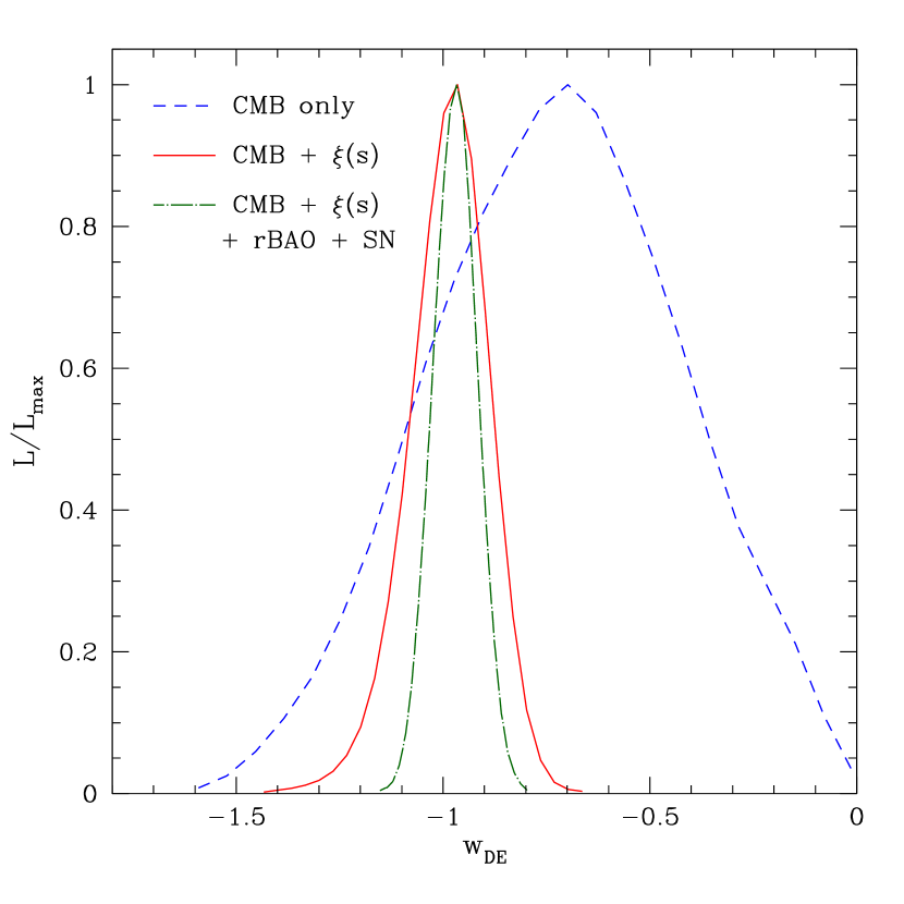
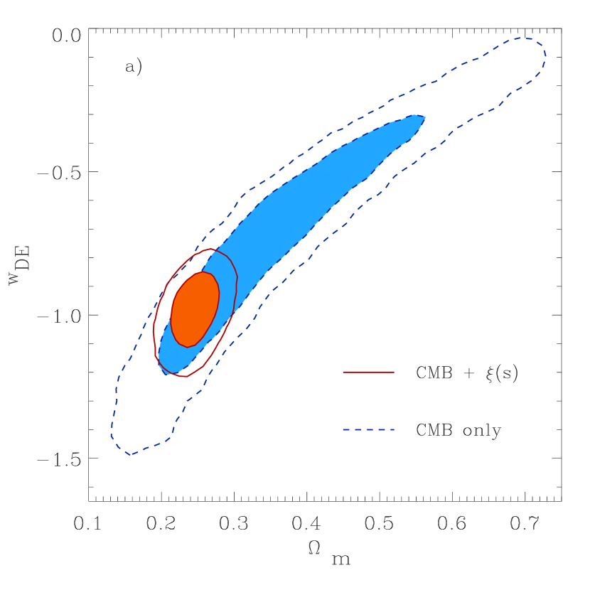
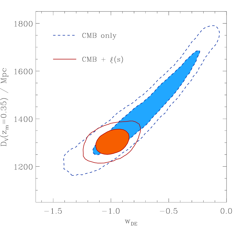
Fig. 7a shows the two-dimensional marginalized constraints in the $\Omega_{\rm m}-w_{\rm DE}$ plane from CMB data alone (dashed lines) and CMB plus the LRG $\xi(s)$. There is a strong degeneracy between these parameters when only CMB data is included in the analysis which leads to poor one-dimensional marginalized constraints of $w_{\rm DE}=-0.73_{-0.30}^{+0.30}$ and $\Omega_{\rm m}=0.36_{-0.12}^{+0.12}$. Another view of this is given by Fig. 8, which shows the one-dimensional marginalized constraint on $w_{\rm DE}$. The CMB only case is again shown by the dashed line.

The origin of this degeneracy is well understood. The position of the acoustic peaks in the CMB power spectrum depends on the size of the sound horizon at the decoupling epoch, $r_{\rm s}(z_{*})$, which is given by Eq. (13). The mapping of the physical scales of the acoustic peaks to angular scales on the sky depends on the comoving angular diameter distance, $D_{\rm A}(z_{*})$, given by Eq. (17). Therefore the peak pattern in the CMB provides tight constraints on the “acoustic scale” given by (Bond et al., 1997; Efstathiou & Bond, 1999; Page et al., 2003; Komatsu et al., 2009)

$$\ell_{\rm A}=\frac{\pi D_{\rm A}(z_{*})}{r_{\rm s}(z_{*})}.$$ (19)

While $w_{\rm DE}$ is relevant for the calculation of $D_{\rm A}(z_{*})$, it has minimum impact on $r_{\rm s}(z_{*})$, since the dark energy is dynamically negligible at decoupling. For this reason, for fixed values of $\omega_{\rm b}$ and $\omega_{\rm dm}$, and given a value of $\Omega_{\rm m}$ (or $h$), it is always possible to find a value of $w_{\rm DE}$ such that the value of $\ell_{\rm A}$ remains constant. This gives rise to the degeneracy between these parameters seen in Fig. 7a.

As shown in Fig. 7a, the inclusion of the LRG correlation function breaks the degeneracy between $\Omega_{\rm m}$ and $w_{\rm DE}$ present in the CMB data. This is done in two ways; first the shape of $\xi(r)$ on intermediate scales tightens the constraints on $\Omega_{\rm m}$, which helps to break the degeneracy between this parameter and $w_{\rm DE}$. Second, through the position of the acoustic peak it provides an independent estimation of the ratio $r_{\rm s}(z_{\rm d})/D_{\rm V}(z_{\rm m})$, where $z_{\rm d}$ is the redshift of the drag epoch and $z_{\rm m}=0.35$ is the mean redshift of the survey.

When this information is combined with the constraint on $r_{\rm s}(z_{\rm d})$ provided by the CMB data, this provides an extra distance measurement, $D_{\rm V}(z_{\rm m}=0.35)$, which breaks the degeneracy in the CMB data. This can be seen more clearly in Fig. 9, which shows the two dimensional constraints in the plane $w_{\rm DE}-D_{\rm V}(z_{\rm m}=0.35)$. Varying $w_{\rm DE}$ to keep a constant value of $\ell_{\rm A}$ produces varying values of $D_{\rm V}(z_{\rm m}=0.35)$. The extra information from the shape of $\xi(s)$ fixes the value of $D_{\rm V}$, tightening the constraints on the dark energy equation of state. In this case we get $\Omega_{\rm m}=0.245_{-0.020}^{+0.021}$ and $w_{\rm DE}=-0.988_{-0.088}^{+0.088}$, in complete agreement with the cosmological constant. Again, Fig. 8 shows the dramatic reduction in the width of the likelihood distribution for $w_{\rm DE}$ on combining the CMB data with the measurement of the LRG correlation function.

Using WMAP data combined with the BAO measurement from Percival et al. (2007c), Komatsu et al. (2009) found $w_{\rm DE}=-1.15_{-0.22}^{+0.21}$ (68% CL). If we exclude the small scale CMB experiments and consider only WMAP measurements plus the LRG $\xi(s)$, we get $w_{\rm DE}=-0.996_{-0.095}^{+0.097}$, which corresponds to a reduction of almost a factor two in the allowed region for the equation of state parameter. This highlights the importance of the information contained in the shape of the correlation function. The method of Percival et al. (2007c) sacrifices the long-wavelength shape of $P(k)$, which is affected by scale-dependent effects, in order to obtain a purely geometrical test from the BAO oscillations.

It is also possible to obtain constraints in this parameter space from the combination of the shape of the LRG $\xi(s)$ with the rBAO data without including any CMB information. In this case we get we get $w_{\rm DE}=-1.05_{-0.15}^{+0.16}$. This means that present day observations allow to obtain a competitive constraint on $w_{\rm DE}$ purely on the basis of large scale structure information, independently of CMB or SN observations.

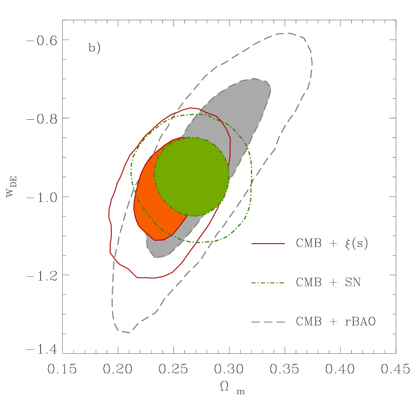
The values of $w_{\rm DE}$ listed in Table 3 as being obtained by combining the CMB data with rBAO and SN information are completely consistent (see Section 7 and Fig. 7b). Once again this shows the consistency between these datasets. Our results including rBAO data show an excellent agreement with those of Gaztañaga et al. (2008c). When including systematic effects in the SN data as advocated by Kowalski et al. (2008), the CMB plus SN result changes to $w_{\rm DE}=-0.900_{-0.078}^{+0.078}$, a 50% increase in the allowed region and a shift in the mean value of $w_{\rm DE}$ of about one $\sigma$. This means that when the SN systematic errors are included in the analysis, the precision of the constraint on $w_{\rm DE}$ obtained from CMB plus SN is comparable to the one derived from CMB plus the shape of the LRG $\xi(s)$. This highlights the importance of using the full shape of $\xi(s)$ as a cosmological probe. This also shows the importance of a precise determination of the effects of systematic errors in the SN data.

5.3 The time evolution of $w_{\rm DE}$

Figure 9: The marginalized posterior likelihood in the $D_{\rm V}-w_{\rm DE}$ plane for the $\Lambda$CDM parameter set extended to allow $w_{\rm DE}$ to vary (Eq. (7)). The dashed lines show the 68 and 95 per cent contours obtained using CMB information alone. The solid contours correspond to the results obtained from the combination of CMB data plus the shape of the LRG $\xi(s)$. The filled contours correspond to the 68% CL in each case.

In the previous section we analysed the possibility of extending the $\Lambda$CDM model with alternative dark energy models with a redshift-independent equation of state. From a theoretical perspective, if $w_{\rm DE}\neq-1$, there is no real reason why it should be constant. In this section, we analyse the constraints on the redshift dependence of this parameter, using the popular linear parametrization of Eq. (4) (Chevallier & Polarski, 2001; Linder et al., 2003).

Figure 10: The marginalized posterior likelihood in the $w_{0}-w_{a}$ plane for the $\Lambda$CDM parameter set extended with a redshift dependent dark energy equation of state parametrized according to Eq. (4). The dashed lines show the 68 and 95 per cent contours obtained using CMB information alone. The solid contours correspond to the results obtained from the combination of CMB data plus the shape of the LRG $\xi(s)$. The dot-dashed contours show the constraints on using all datasets. The filled contours correspond to the 68% CL in each case. The dotted straight line marks the degeneracy between $w_{0}$ and $w_{a}$.

Figure 11: The marginalized posterior likelihood in $w_{\rm DE}$ as a function of $z$ for the $\Lambda$CDM parameter set extended with a redshift dependent dark energy equation of state parametrized as in Eq. (4). The dashed lines show the mean value (thick line) and the corresponding 68 per cent constraints (filled blue region between thin lines) obtained using CMB information alone. The solid lines (and filled orange region) show the corresponding results from the combination of CMB plus the shape of the LRG $\xi(s)$. The dotted vertical line corresponds to the pivot redshift $z_{\rm p}=0.39$.

This parametrization may lead to models in which the dark energy density has a dynamical impact at the epoch of Big Bang Nucleosynthesis (BBN), unlike the case with a cosmological constant. Such a scenario would affect the present day abundances of light elements, thereby violating the constraints on the possible variation in the Hubble parameter at the epoch of BBN as expressed through the ratio (Steigman, 2007):

$$S\equiv\frac{H^{\prime}(a_{\rm BBN})}{H(a_{\rm BBN})}=0.942\pm 0.030,$$ (20)

where $H(a_{\rm BBN})$ is the Hubble parameter in a standard $\Lambda$CDM model, in which case dark energy is completely negligible at the expansion factor corresponding to the epoch of Big Bang nucleosynthesis, $a_{\rm BBN}$, and $H^{\prime}(a_{\rm BBN})$ is the Hubble parameter at the same epoch in an alternative model in which dark energy does play a role at this early epoch. Here we follow Wright (2007) and Komatsu et al. (2009) and impose a Gaussian prior given by Eq. (20) on $S$ which can be written as

$$S=\sqrt{1+\frac{\Omega_{\rm DE}\,a_{\rm BBN}^{-3(1+w_{\rm eff}(z_{\rm BBN}))}}{\Omega_{\rm m}\,a_{\rm BBN}^{-3}+\Omega_{\rm r}\,a_{\rm BBN}^{-4}+\Omega_{k}\,a_{\rm BBN}^{-2}}},$$ (21)

where $a_{\rm BBN}=10^{-9}$ and $w_{\rm eff}$ is the effective dark energy equation of state, defined as

$$w_{\rm eff}(a)\equiv\frac{1}{\ln(a)}\int_{0}^{\ln(a)}w_{\rm DE}(a^{\prime})\,{\rm d}\ln a^{\prime}.$$ (22)

With the parametrization of Eq. (4) this becomes

$$w_{\rm eff}(a)=w_{0}+w_{a}\left(1+\frac{1-a}{\ln(a)}\right).$$ (23)

Table 4 summarizes the constraints obtained in this parameter space using different combinations of datasets.

Table 4: The marginalized 68% interval constraints on cosmological parameters allowing for an evolving dark energy equation of state (i.e. the parameter set defined by Eq.(8)), obtained using different combinations of the datasets described in Section 2, as stated in the column headings.

	CMB	CMB + $\xi(s)$	CMB + rBAO	CMB + SN	CMB + $\xi(s)$	CMB + $\xi(s)$	$\xi(s)$+ rBAO
					+ rBAO	+ rBAO + SN
$w_{\rm 0}$	$-0.68_{-0.48}^{+0.48}$	$-1.00_{-0.29}^{+0.29}$	$-0.85_{-0.49}^{+0.49}$	$-1.07_{-0.15}^{+0.16}$	$-1.10_{-0.19}^{+0.19}$	$-1.03_{-0.10}^{+0.10}$	$-1.06_{-0.18}^{+0.19}$
$w_{a}$	$-0.30_{-0.96}^{+0.96}$	$-0.065_{-1.02}^{+0.99}$	$-0.2_{-1.0}^{+1.0}$	$0.45_{-0.61}^{+0.59}$	$0.31_{-0.59}^{+0.60}$	$0.30_{-0.41}^{+0.41}$	$-0.0_{-1.1}^{+0.9}$
$100\Theta$	$1.0413_{-0.0023}^{+0.0023}$	$1.0416_{-0.0023}^{+0.0023}$	$1.0415_{-0.0022}^{+0.0022}$	$1.0413_{-0.0022}^{+0.0022}$	$1.0414_{-0.0022}^{+0.0022}$	$1.0416_{-0.0022}^{+0.0022}$	$0.997_{-0.078}^{+0.073}$
$\omega_{\rm dm}$	$0.1098_{-0.0054}^{+0.0054}$	$0.1076_{-0.0050}^{+0.0051}$	$0.1098_{-0.0044}^{+0.0043}$	$0.1107_{-0.0052}^{+0.0053}$	$0.1087_{-0.0047}^{+0.0047}$	$0.1077_{-0.0045}^{+0.0045}$	$0.096_{-0.045}^{+0.048}$
$100\,\omega_{\rm b}$	$2.270_{-0.052}^{+0.051}$	$2.284_{-0.052}^{+0.053}$	$2.279_{-0.051}^{+0.051}$	$2.271_{-0.053}^{+0.053}$	$2.278_{-0.051}^{+0.051}$	$2.280_{-0.051}^{+0.050}$	$2.6_{-1.5}^{+1.6}$
$\tau$	$0.090_{-0.017}^{+0.017}$	$0.090_{-0.017}^{+0.017}$	$0.090_{-0.017}^{+0.017}$	$0.089_{-0.017}^{+0.017}$	$0.089_{-0.017}^{+0.017}$	$0.091_{-0.017}^{+0.016}$	-
$n_{\rm s}$	$0.961_{-0.013}^{+0.013}$	$0.966_{-0.013}^{+0.013}$	$0.964_{-0.012}^{+0.012}$	$0.960_{-0.013}^{+0.013}$	$0.963_{-0.012}^{+0.012}$	$0.963_{-0.012}^{+0.012}$	$1.04_{-0.32}^{+0.32}$
$\ln(10^{10}A_{\rm s})$	$3.065_{-0.038}^{+0.038}$	$3.059_{-0.037}^{+0.038}$	$3.068_{-0.038}^{+0.038}$	$3.068_{-0.037}^{+0.037}$	$3.061_{-0.037}^{+0.037}$	$3.062_{-0.037}^{+0.036}$	-
$\Omega_{\rm DE}$	$0.66_{-0.11}^{+0.11}$	$0.755_{-0.023}^{+0.023}$	$0.715_{-0.062}^{+0.062}$	$0.718_{-0.024}^{+0.024}$	$0.749_{-0.018}^{+0.018}$	$0.738_{-0.013}^{+0.013}$	$0.780_{-0.047}^{+0.045}$
$\Omega_{\rm m}$	$0.34_{-0.11}^{+0.11}$	$0.245_{-0.023}^{+0.023}$	$0.285_{-0.062}^{+0.062}$	$0.282_{-0.024}^{+0.024}$	$0.251_{-0.018}^{+0.018}$	$0.262_{-0.013}^{+0.013}$	$0.220_{-0.045}^{+0.047}$
$\sigma_{8}$	$0.733_{-0.082}^{+0.084}$	$0.786_{-0.045}^{+0.045}$	$0.773_{-0.070}^{+0.071}$	$0.7790_{-0.041}^{+0.041}$	$0.791_{-0.048}^{+0.047}$	$0.769_{-0.040}^{+0.040}$	-
$t_{0}/{\rm Gyr}$	$13.89_{-0.31}^{+0.32}$	$13.65_{-0.18}^{+0.19}$	$13.72_{-0.14}^{+0.14}$	$13.83_{-0.17}^{+0.18}$	$13.72_{-0.13}^{+0.13}$	$13.76_{-0.12}^{+0.12}$	$14.6_{-3.0}^{+3.3}$
$z_{\rm re}$	$10.6_{-1.4}^{+1.4}$	$10.5_{-1.3}^{+1.4}$	$10.5_{-1.4}^{+1.4}$	$10.6_{-1.4}^{+1.4}$	$10.5_{-1.4}^{+1.4}$	$10.6_{-1.3}^{+1.3}$	-
$h$	$0.65_{-0.10}^{+0.10}$	$0.732_{-0.031}^{+0.028}$	$0.692_{-0.075}^{+0.078}$	$0.689_{-0.023}^{+0.023}$	$0.726_{-0.027}^{+0.025}$	$0.706_{-0.015}^{+0.015}$	$73_{-0.14}^{+0.16}$

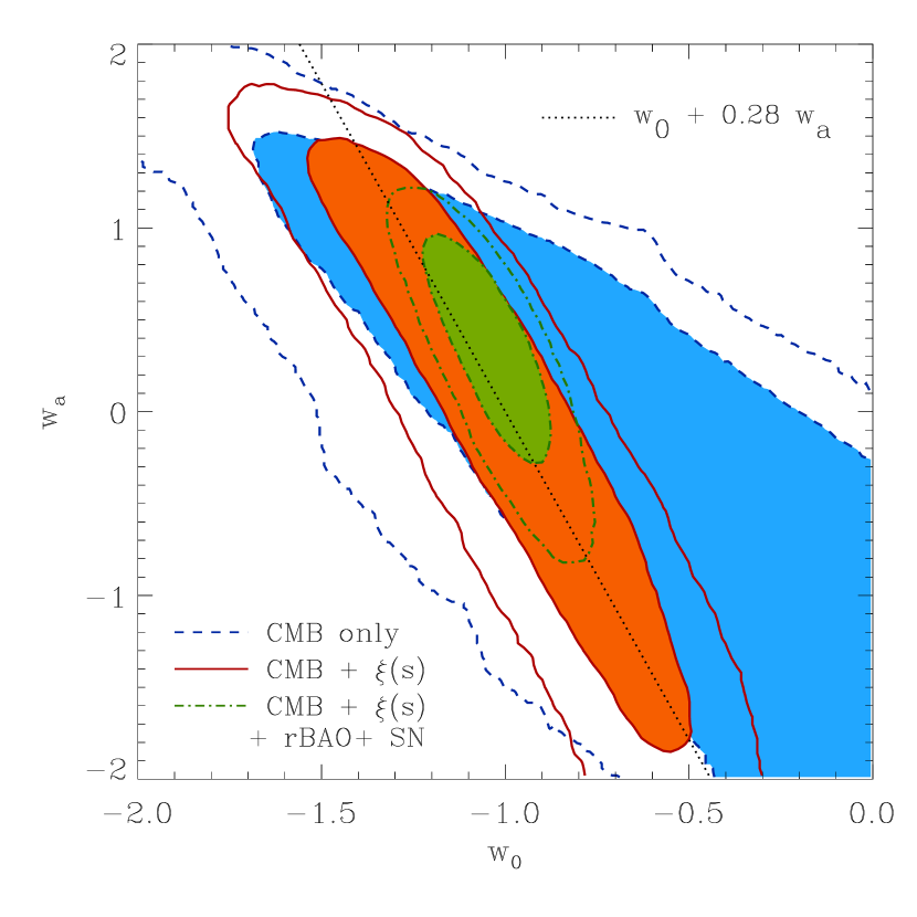
The dashed lines in Fig. 10 show the two dimensional marginalized constraints in the $w_{0}-w_{a}$ plane from CMB data alone. As discussed in the previous section, the CMB data follows a degeneracy of constant $\ell_{\rm A}$. Allowing the dark energy to evolve with redshift, this degeneracy gains an extra degree of freedom leading to poor constraints on $w_{0}$ and $w_{a}$.

These constraints can be transformed into constraints on the value of $w_{\rm DE}(a)$ which will be given by

$$\langle\delta w_{\rm DE}(a)^{2}\rangle=\langle(\delta w_{\rm 0}+(1-a)\delta w_{\rm a})^{2}\rangle.$$ (24)

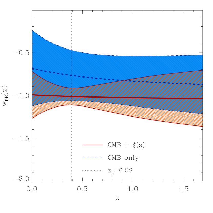
The dashed lines in Fig. 11 show the mean value of $w_{\rm DE}(z)$ as a function of $z$ (thick line), as well as the 68 per cent confidence limits (thin lines) obtained from CMB data alone. These constraints can accommodate large variations of $w_{\rm DE}(z)$. The solid lines show the correspondent results when the LRG correlation function is included in the analysis. Although considerable deviations from the simple cosmological constant case are still allowed, these are much strongly constrained by the data.

The pivot scale factor $a_{\rm p}$ is defined as the point where Eq. (24) is minimized (Huterer & Turner, 2001; Hu & Jain, 2004; Albretch et al., 2006). That is

$$a_{\rm p}=1+\frac{\langle\delta w_{\rm 0}\delta w_{\rm a}\rangle}{\langle\delta w_{\rm a}^{2}\rangle}.$$ (25)

For the combination of CMB plus the shape of $\xi(s)$ the corresponding pivot redshift is given by $z_{\rm p}=0.39$, which is shown by the dotted line in Fig. 11. At this redshift we get our tightest constraint on the dark energy equation of state, with $w_{\rm DE}(z_{\rm p}=0.39)=-1.01\pm 0.10$, entirely consistent with a cosmological constant. In this case also, adding the information from the shape of $\xi(s)$ allows to obtain a tight constraint on $\Omega_{\rm m}=0.245_{-0.022}^{+0.023}$.

The solid lines in Fig. 10 show the two dimensional marginalized constraints in the $w_{0}-w_{a}$ plane for CMB plus the shape of $\xi(s)$. The constraint on $w_{\rm DE}(z_{\rm p}=0.39)$ corresponds to a degeneracy between these parameters approximately given by $w_{\rm 0}+0.28w_{\rm a}=-1$, which is shown by the dotted line in Fig. 10.

Adding information from rBAO or SN gives completely consistent results, which are shown by the dot-dashed lines in Fig. 10. The combination of all the datasets gives the tightest constraints, with $w_{0}=-1.03\pm 0.10$, $w_{a}=0.30_{-0.41}^{+0.41}$ and $\Omega_{\rm m}=0.262\pm 0.013$. These values correspond to a lower pivot redshift $z_{\rm p}=0.28$ for which we get $w_{\rm DE}(z_{\rm p}=0.28)=-0.969\pm 0.049$. Even allowing for dynamic dark energy models current observations can constrain the present value of $w_{\rm DE}$ at the 10% level.

Combining the shape of the LRG correlation function with the rBAO measurements we obtain the constraints $w_{0}=-1.06_{-0.18}^{+0.19}$ and $w_{a}=0.0_{-1.1}^{+0.9}$. These constraints give a much lower pivot redshift, with $z_{\rm p}=0.11$, for which we find $w_{\rm DE}(z_{\rm p}=0.11)=-1.06\pm 0.19$. This shows that current large scale structure data allows for the present value of a redshift-dependent dark energy equation of state to be determined at the 20$\%$ level.

5.4 Non-flat models

Figure 12: The marginalized posterior likelihood in the $\Omega_{\rm m}-\Omega_{\rm DE}$ plane for the $\Lambda$CDM parameter set extended with $\Omega_{k}$ (Eq. (9)). The dashed lines show the 68 and 95 per cent contours obtained using CMB information alone. The solid contours correspond to the results obtained from the combination of CMB with the shape of the LRG $\xi(s)$. The thick solid line corresponds to flat models, where $\Omega_{k}=0$. The filled contours correspond to the 68% CL in each case.

Table 5: The marginalized 68% interval constraints on cosmological parameters for non-flat $\Lambda$CDM models (i.e. the parameter set defined by Eq.(9)), obtained using different combinations of the datasets described in Section 2, as stated in the column headings.

	CMB	CMB + $\xi(s)$	CMB + rBAO	CMB + SN	CMB + $\xi(s)$	CMB + $\xi(s)$	$\xi(s)$+ rBAO
					+ rBAO	+ rBAO + SN
$\Omega_{k}$	$-0.064_{-0.063}^{+0.056}$	$-0.0016_{-0.0074}^{+0.0070}$	$-0.0036_{-0.0053}^{+0.0053}$	$-0.012_{-0.010}^{+0.010}$	$-0.0034_{-0.0051}^{+0.0051}$	$-0.0035_{-0.0051}^{+0.0050}$	$-0.12_{-0.088}^{+0.089}$
$100\,\Theta$	$1.0412_{-0.0023}^{+0.0022}$	$1.0415_{-0.0022}^{+0.0022}$	$1.0415_{-0.0022}^{+0.0022}$	$1.0414_{-0.0023}^{+0.0022}$	$1.0415_{-0.0022}^{+0.0022}$	$1.0415_{-0.0023}^{+0.0023}$	$1.40_{-0.34}^{+0.34}$
$\omega_{\rm dm}$	$0.1104_{-0.0050}^{+0.0050}$	$0.1064_{-0.0048}^{+0.0048}$	$0.1086_{-0.0046}^{+0.0047}$	$0.1080_{-0.0048}^{+0.0047}$	$0.1072_{-0.0047}^{+0.0046}$	$0.1084_{-0.0044}^{+0.0044}$	$0.112_{-0.049}^{+0.051}$
$100\,\omega_{\rm b}$	$2.253_{-0.051}^{+0.049}$	$2.275_{-0.051}^{+0.051}$	$2.272_{-0.051}^{+0.051}$	$2.266_{-0.051}^{+0.050}$	$2.274_{-0.050}^{+0.050}$	$2.267_{-0.050}^{+0.050}$	$3.1_{-1.6}^{+1.7}$
$\tau$	$0.087_{-0.017}^{+0.017}$	$0.089_{-0.017}^{+0.017}$	$0.090_{-0.018}^{+0.017}$	$0.090_{-0.017}^{+0.017}$	$0.089_{-0.017}^{+0.017}$	$0.088_{-0.016}^{+0.016}$	-
$n_{\rm s}$	$0.956_{-0.013}^{+0.012}$	$0.964_{-0.012}^{+0.012}$	$0.963_{-0.012}^{+0.012}$	$0.960_{-0.012}^{+0.012}$	$0.963_{-0.012}^{+0.012}$	$0.961_{-0.012}^{+0.012}$	$0.99_{-0.31}^{+0.32}$
$\ln(10^{10}A_{\rm s})$	$3.061_{-0.037}^{+0.037}$	$3.052_{-0.037}^{+0.038}$	$3.062_{-0.039}^{+0.038}$	$3.058_{-0.038}^{+0.038}$	$3.055_{-0.038}^{+0.037}$	$3.055_{-0.035}^{+0.035}$	-
$\Omega_{\rm DE}$	$0.56_{-0.17}^{+0.16}$	$0.756_{-0.021}^{+0.021}$	$0.740_{-0.018}^{+0.018}$	$0.717_{-0.023}^{+0.023}$	$0.748_{-0.015}^{+0.015}$	$0.741_{-0.013}^{+0.013}$	$0.894_{-0.090}^{+0.091}$
$\Omega_{\rm m}$	$0.498_{-0.22}^{+0.23}$	$0.245_{-0.024}^{+0.025}$	$0.263_{-0.018}^{+0.019}$	$0.295_{-0.030}^{+0.030}$	$0.256_{-0.015}^{+0.016}$	$0.262_{-0.013}^{+0.013}$	$0.226_{-0.047}^{+0.049}$
$\sigma_{8}$	$0.765_{-0.032}^{+0.032}$	$0.778_{-0.028}^{+0.028}$	$0.791_{-0.028}^{+0.028}$	$0.782_{-0.028}^{+0.028}$	$0.782_{-0.027}^{+0.027}$	$0.787_{-0.026}^{+0.026}$	-
$t_{0}/{\rm Gyr}$	$15.7_{-1.6}^{+1.6}$	$13.71_{-0.38}^{+0.39}$	$13.85_{-0.26}^{+0.26}$	$14.27_{-0.46}^{+0.46}$	$13.83_{-0.25}^{+0.25}$	$13.85_{-0.25}^{+0.25}$	$14.2_{-2.6}^{+2.9}$
$z_{\rm re}$	$10.3_{-1.4}^{+1.4}$	$10.4_{-1.3}^{+1.3}$	$10.5_{-1.4}^{+1.4}$	$10.49_{-1.4}^{+1.3}$	$10.4_{-1.4}^{+1.3}$	$10.3_{-1.3}^{+1.3}$	-
$h$	$0.55_{-0.15}^{+0.13}$	$0.730_{-0.037}^{+0.034}$	$0.707_{-0.021}^{+0.021}$	$0.668_{-0.037}^{+0.037}$	$0.713_{-0.019}^{+0.019}$	$0.707_{-0.017}^{+0.017}$	$0.78_{-0.14}^{+0.15}$

The flatness of the Universe is one of the generic predictions of most common models of inflation. A detection of a non-negligible curvature would have profound implications for our understanding of the mechanism thought to be responsible for seeding density fluctuations in the Universe. The flatness hypothesis is also important because it has a strong impact on the constraints on the remaining cosmological parameters, since many of them are degenerate with $\Omega_{k}$. In this section, we analyse non-flat models and include $\Omega_{k}$ in our parameter space, assuming that the dark energy is given by vacuum energy with $w_{\rm DE}=-1$.

Figure 13: The marginalized posterior likelihood in $\Omega_{\rm k}$ for the $\Lambda$CDM parameter set extended with $\Omega_{k}$ (Eq. (9)). The dashed line shows the likelihood obtained using CMB information alone. The solid line corresponds to the result obtained from the combination of CMB data with the shape of the LRG $\xi(s)$. The dot-dashed line shows the likelihood when all datasets are considered.

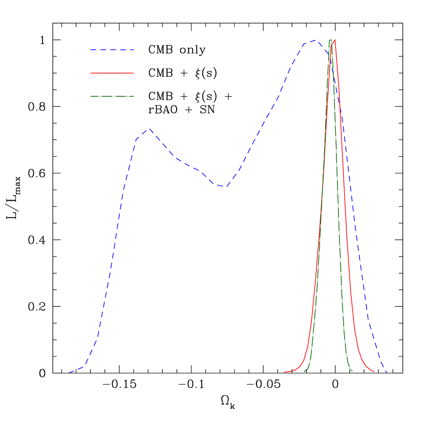
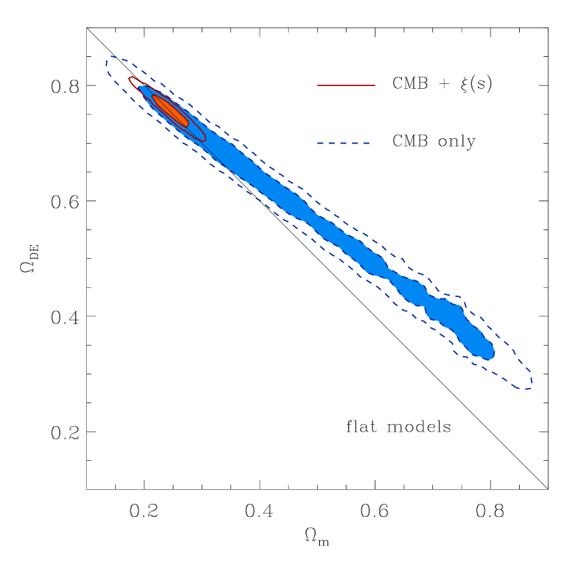
When $\Omega_{k}$ is allowed to float, the CMB data alone are unable to constrain all the parameters at the same time, giving rise to the well known geometrical degeneracy, which is completely analogous to the one between $w_{\rm DE}$ and $\Omega_{\rm m}$ described in Section 5.2. For each choice of $\omega_{\rm b}$, $\omega_{\rm dm}$ and $\Omega_{\rm m}$, it is possible to find a value of $\Omega_{k}$ (or $\Omega_{\rm DE}$) which will give the same value of $\ell_{\rm A}$. This strong degeneracy can be seen in the dashed lines of Fig. 12, which shows the two dimensional marginalized constraints in the plane $\Omega_{\rm m}-\Omega_{\rm DE}$. We plot the marginalized constraints on $\Omega_{k}$ in Fig. 13. The dashed curve shows the results for CMB data alone. This narrow degeneracy produces poor marginalized constraints on the curvature of the Universe, with $\Omega_{k}=-0.064_{-0.063}^{+0.056}$.

Adding the independent constraint from the shape of the LRG $\xi(s)$ helps to break this degeneracy. The solid lines in Fig. 12 show how with this extra information the two dimensional constraints in the plane $\Omega_{\rm m}-\Omega_{\rm DE}$ close up over the locus of the flat models (shown by the thick solid line). From CMB data plus the LRG $\xi(s)$ we get $\Omega_{k}=-0.0016_{-0.0074}^{+0.0070}$. Combining the CMB data with the other external datasets yields similar results, with $\Omega_{k}=-0.012_{-0.010}^{+0.010}$ for CMB plus SN and $\Omega_{k}=-0.0036_{-0.0053}^{+0.0053}$ from CMB plus rBAO.

Figure 14: The marginalized posterior likelihood in the $\Omega_{k}-w_{\rm DE}$ plane for the $\Lambda$CDM parameter set extended with $\Omega_{k}$ and $w_{\rm DE}$ (Eq. (3)). The dashed lines show the 68 and 95 per cent contours obtained using CMB information alone. The solid contours correspond to the results obtained from the combination of CMB data with the shape of the LRG $\xi(s)$. The dot-dashed lines show the constraints obtained using all data sets. The filled contours correspond to the 68% CL in each case.

The combination of the shape of the LRG $\xi(s)$ and the rBAO data is not able to give meaningful constraints on $\Omega_{k}$. This data combination allows for a wide range of closed models giving a very poor one dimensional marginalized constraint of $\Omega_{k}=-0.12_{-0.088}^{+0.089}$. On the other hand, these datasets can give a constraint on the matter density of $\Omega_{\rm m}=0.226_{-0.047}^{+0.049}$, with a similar precision to the one obtained in the parameter spaces analysed in the previous sections.

Our tightest constraint comes from the combination of the four datasets, which gives $\Omega_{k}=-0.0035_{-0.0050}^{+0.0051}$, which is dominated by the combination of CMB and rBAO data. This result is in full agreement with that found by Komatsu et al. (2009) from the combination of WMAP-5yr data with the BAO measurements from Percival et al. of $\Omega_{k}=-0.0050_{-0.0060}^{+0.0061}$. This means that, with the hypothesis that vacuum energy is the source of the accelerated expansion of the Universe, current data allow us to probe spatial curvature up to $\Omega_{\rm k}\simeq 5\times 10^{-3}$. As we shall see in Section 5.5, this limit does not change when the assumption of $w_{\rm DE}=-1$ is relaxed.

Table 6: The marginalized 68% interval constraints on the cosmological parameters allowing for non-flat models and variations in the (redshift independent) dark energy equation of state parameter (i.e. the parameter space defined by Eq. (3)), obtained using different combinations of the datasets described in Section 2, as stated in the column headings.

	CMB	CMB + $\xi(s)$	CMB + rBAO	CMB + SN	CMB + $\xi(s)$	CMB + $\xi(s)$	$\xi(s)$+ rBAO
					+ rBAO	+ rBAO + SN
$\Omega_{k}$	$-0.045_{-0.073}^{+0.067}$	$0.040_{-0.060}^{+0.057}$	$0.0089_{-0.016}^{+0.014}$	$-0.046_{-0.032}^{+0.037}$	$-0.0034_{-0.0065}^{+0.0065}$	$-0.0018_{-0.0054}^{+0.0054}$	$-0.169_{-0.092}^{+0.099}$
$w_{\rm DE}$	$-0.98_{-0.67}^{+0.57}$	$-0.81_{-0.48}^{+0.39}$	$-0.83_{-0.29}^{+0.29}$	$-1.31_{-0.34}^{+0.37}$	$-1.03_{-0.12}^{+0.12}$	$-0.965_{-0.081}^{+0.078}$	$-0.91_{-0.14}^{+0.13}$
$100\,\Theta$	$1.0411_{-0.0022}^{+0.0023}$	$1.0412_{-0.0022}^{+0.0022}$	$1.0415_{-0.0022}^{+0.0022}$	$1.0413_{-0.0023}^{+0.0022}$	$1.0416_{-0.0022}^{+0.0022}$	$1.0415_{-0.0022}^{+0.0022}$	$1.58_{-0.42}^{+0.39}$
$\omega_{\rm dm}$	$0.1104_{-0.0051}^{+0.0049}$	$0.1057_{-0.0049}^{+0.0050}$	$0.1085_{-0.0048}^{+0.0048}$	$0.1094_{-0.0047}^{+0.0048}$	$0.1073_{-0.0046}^{+0.0046}$	$0.1078_{-0.0046}^{+0.0047}$	$0.106_{-0.043}^{+0.045}$
$100\,\omega_{\rm b}$	$2.254_{-0.054}^{+0.052}$	$2.259_{-0.048}^{+0.049}$	$2.270_{-0.051}^{+0.050}$	$2.257_{-0.052}^{+0.050}$	$2.274_{-0.050}^{+0.050}$	$2.270_{-0.046}^{+0.046}$	$0.030_{-0.016}^{+0.018}$
$\tau$	$0.087_{-0.017}^{+0.017}$	$0.089_{-0.017}^{+0.017}$	$0.090_{-0.017}^{+0.017}$	$0.087_{-0.017}^{+0.017}$	$0.089_{-0.017}^{+0.017}$	$0.088_{-0.017}^{+0.017}$	-
$n_{\rm s}$	$0.956_{-0.013}^{+0.013}$	$0.963_{-0.013}^{+0.013}$	$0.962_{-0.012}^{+0.012}$	$0.957_{-0.012}^{+0.012}$	$0.963_{-0.012}^{+0.012}$	$0.962_{-0.012}^{+0.012}$	$0.99_{-0.30}^{+0.31}$
$\ln(10^{10}A_{\rm s})$	$3.059_{-0.038}^{+0.037}$	$3.047_{-0.038}^{+0.037}$	$3.061_{-0.038}^{+0.037}$	$3.057_{-0.037}^{+0.039}$	$3.055_{-0.039}^{+0.038}$	$3.055_{-0.037}^{+0.036}$	-
$\Omega_{\rm DE}$	$0.54_{-0.16}^{+0.15}$	$0.726_{-0.034}^{+0.033}$	$0.697_{-0.065}^{+0.066}$	$0.649_{-0.054}^{+0.058}$	$0.750_{-0.020}^{+0.019}$	$0.740_{-0.013}^{+0.013}$	$0.94_{-0.10}^{+0.09}$
$\Omega_{\rm m}$	$0.50_{-0.20}^{+0.22}$	$0.233_{-0.041}^{+0.047}$	$0.294_{-0.052}^{+0.052}$	$0.397_{-0.093}^{+0.087}$	$0.253_{-0.017}^{+0.017}$	$0.260_{-0.013}^{+0.013}$	$0.23_{-0.044}^{+0.044}$
$\sigma_{8}$	$0.73_{-0.10}^{+0.10}$	$0.667_{-0.15}^{+0.17}$	$0.735_{-0.091}^{+0.090}$	$0.805_{-0.045}^{+0.047}$	$0.789_{-0.046}^{+0.046}$	$0.775_{-0.033}^{+0.034}$	-
$t_{0}/{\rm Gyr}$	$15.4_{-1.9}^{+1.9}$	$12.6_{-1.8}^{+2.1}$	$13.67_{-0.38}^{+0.38}$	$15.6_{-1.4}^{+1.2}$	$13.85_{-0.31}^{+0.30}$	$13.78_{-0.26}^{+0.26}$	$14.3_{-2.6}^{+2.7}$
$z_{\rm re}$	$10.4_{-1.5}^{+1.5}$	$10.9_{-1.6}^{+1.6}$	$10.7_{-1.4}^{+1.4}$	$10.2_{-1.4}^{+1.4}$	$10.4_{-1.4}^{+1.4}$	$10.4_{-1.3}^{+1.3}$	-
$h$	$0.54_{-0.14}^{+0.12}$	$0.750_{-0.068}^{+0.061}$	$0.676_{-0.060}^{+0.060}$	$0.589_{-0.066}^{+0.070}$	$0.718_{-0.025}^{+0.024}$	$0.706_{-0.017}^{+0.017}$	$0.76_{-0.13}^{+0.14}$

5.5 Dark energy and curvature

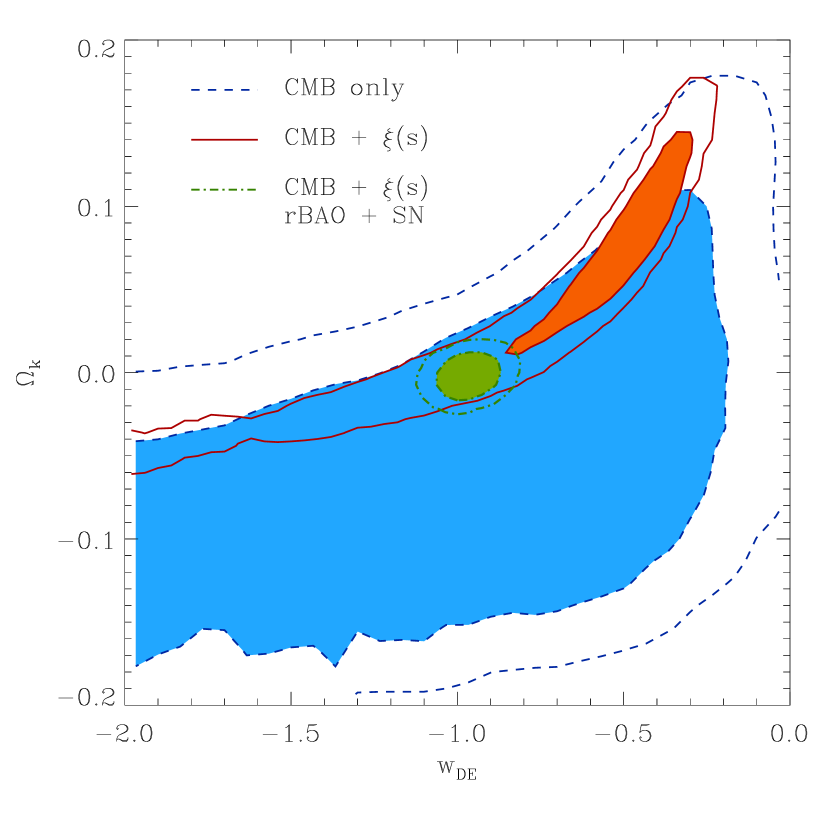
The assumption of a flat Universe has important implications for the constraints on the dark energy equation of state. Neither the curvature nor the dark energy play a role in determining the physical scales of the acoustic peaks in the CMB. These quantities do, however, have an impact on the angular diameter distance to the decoupling epoch. Furthermore, their contribution is degenerate. An increment in the value of $\Omega_{k}$, which reduces the value of $D_{\rm A}(z_{*})$, can be compensated for by an increase in $w_{\rm DE}$, which produces the opposite effect. This means that, instead of a one dimensional degeneracy as in the cases analysed in Sections 5.2 and 5.4, this parameter space has an extra degree of freedom for every choice of $\omega_{\rm b}$, $\omega_{\rm dm}$ and $\Omega_{\rm m}$. Fig. 14 shows the marginalized posterior likelihood in the $w_{\rm DE}-\Omega_{k}$ plane. Due to this degeneracy, the region allowed by the CMB data, shown by the dashed lines, covers a wide range of this parameter space. When the information from the shape of the correlation function is included in the analysis, the extra distance measurement reduces this degeneracy to an (approximately) one dimensional region in the $w_{\rm DE}-\Omega_{k}$ plane shown by the solid lines, but is also unable to place meaningful constraints on these parameters.

An extra piece of information, coming from rBAO or SN data can break the remaining degeneracy. The dot-dashed lines in Fig. 14 correspond to the results obtained by combining the CMB measurements, the SDSS $\xi(s)$, rBAO and SN data. Combining all these datasets, the contours close-up over the canonical $\Lambda$CDM values, with $\Omega_{k}=-0.0018_{-0.0054}^{+0.0054}$ and $w_{\rm DE}=-0.965_{-0.053}^{+0.054}$ It is important to note that the precision of these constraints is similar to those obtained with the assumptions of a flat Universe (Section 5.2) or a cosmological constant (Section 5.4), showing the robustness of our results.

As in Sec. 5.4, the combination of the LRG $\xi(s)$ and the rBAO measurements is not able to give useful constraints in this parameter space. In this case, there is a wide range of closed models allowed by the data, which leads to a poor marginalized constraint of $\Omega_{k}=-0.169_{-0.092}^{+0.099}$. On the other hand, the large scale structure data is able to constrain the dark energy equation of state to $w_{\rm DE}=-0.91\pm 0.14$, with the same level of accuracy obtained with the assumption of a flat Universe.

6 Distance constraints

In this section we explore the distance measurements that can be obtained from the shape of the LRG redshift space correlation function and its combination with other datasets. For the results of this section we have imposed the conservative constraint on the LRG bias factor of $b<4$.

Figure 15: The marginalized posterior likelihood in the $D_{\rm A}(z_{\rm m}=0.35)-H(z_{\rm m}=0.35)$ plane for the $\Lambda$CDM parameter set extended with $\Omega_{k}$ and $w_{\rm DE}$ (Eq. (3)). The short-dashed and long-dashed lines show the 68 and 95 per cent contours obtained individually from CMB information and the LRG $\xi(s)$ respectively. The solid contours correspond to the results obtained from the combination of CMB data plus the shape of the LRG $\xi(s)$, which follow approximately a line of constant $G(z_{\rm m}=0.35)$ (dotted line) defined by Eq. (28). The dot-dashed lines show the contours obtained including also rBAO information. The shading fills the 68% CL contours.

Eisenstein et al. (2005) used the correlation function of a sample of around 46,000 LRGs from the SDSS to obtain constraints on $\Omega_{\rm m}h^{2}$ and the combinations of distance measurements $D_{\rm V}(z)$ (defined in Eq. 16) and $A(z)$, defined as

$$A(z)\equiv D_{\rm V}(z)\frac{\sqrt{\Omega_{\rm m}H_{0}^{2}}}{zc},$$ (26)

at the mean redshift of the survey $z_{\rm m}=0.35$ and found $D_{\rm V}(z_{\rm m}=0.35)=1370\pm 64\,{\rm Mpc}$ and $A(z_{\rm m}=0.35)=0.469\pm 0.017$. In their analysis, Eisenstein et al. (2005) fixed the values of $w_{\rm b}=0.0223$ and $n_{s}=0.98$, as well as adopting a fixed BAO damping scale $k_{\star}=0.11\,h\,{\rm Mpc}^{-1}$ and varied only $\Omega_{\rm m}h^{2}$ and $D_{\rm V}(z_{\rm m}=0.35)$. Fixing the values of these parameters has implications for the obtained constraints. They also implemented a different model for the non-linear distortion of the shape of the correlation function and included a wider range of scales in their analysis ($10\,h^{-1}{\rm Mpc}<r<177\,h^{-1}{\rm Mpc}$) than we consider. Eisenstein et al. (2005) used a fixed template for the nonlinear distortion of the linear perturbation theory correlation function, ignoring changes expected on varying the cosmological parameters (e.g. $\sigma_{8}$). Also, no attempt was made to model scale dependent effects such as redshift space distortions or bias, which could become important for pair separations approaching $10h^{-1}\,$Mpc. In our analysis, we only consider pair separations given by $r>42.5\,h^{-1}{\rm Mpc}$, for which our theoretical model is in excellent agreement with the results of N-body simulations (see Fig. 3). For the wide priors listed in Table 1, and using only information from the shape of $\xi(s)$ over the range of pair separations $42.5\,h^{-1}{\rm Mpc}<r<150\,h^{-1}{\rm Mpc}$, we find weaker constraints, $D_{\rm V}(z_{\rm m}=0.35)=1230\pm 220\,{\rm Mpc}$ and $A(z_{\rm m}=0.35)=0.424\pm 0.064$. To achieve an accuracy comparable to that of Eisenstein et al. it is necessary to combine the $\xi(s)$ constraints with CMB information. In this case we find $D_{\rm V}(z_{\rm m}=0.35)=1300\pm 31\,{\rm Mpc}$ and $A(z_{\rm m}=0.35)=0.447\pm 0.015$.

In the analysis of the fifth year data of the WMAP satellite, Komatsu et al. (2009) produced a set of distance priors that contain most of the information in the WMAP power spectrum. This set contains (i) the physical baryon density $w_{\rm b}$, (ii) the redshift to the decoupling epoch $z_{*}$, (iii) the “acoustic scale” of Eq. (19) and (iv) the “shift parameter” $R$ given by

$$R(z_{*})\equiv D_{\rm A}(z_{*})\frac{\sqrt{\Omega_{\rm m}H_{0}^{2}}}{c},$$ (27)

with their respective covariance matrix. Here, we provide an extended set of distance priors combining the information from the clustering of the LRGs with CMB data. For this, we expand the set of parameters provided by Komatsu et al. (2009) by adding an extra constraint on the quantity

$$G(z_{\rm m})\equiv D_{\rm A}(z_{\rm m})\times h(z_{\rm m})^{0.8},$$ (28)

where $h(z_{\rm m})=H(z_{\rm m})/100\,{\rm km\,s^{-1}\,Mpc^{-1}}$. Now we show that this parameter is well constrained by the combination of the CMB measurements and the LRG $\xi(s)$.

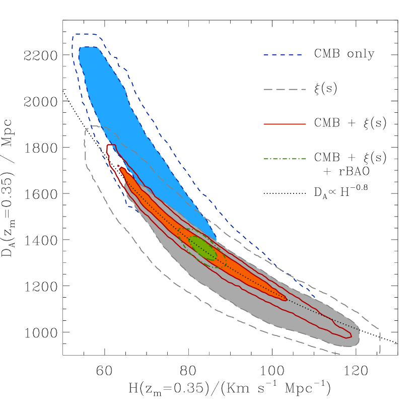
Fig. 15 shows the marginalized posterior likelihood in the $D_{\rm A}(z_{\rm m})-H(z_{\rm m})$ plane for the full parameter space of Eq. (3). The constraints obtained individually from CMB information (short-dashed lines) and the LRG $\xi(s)$ (long-dashed lines) show strong degeneracies between these parameters. The combination of the two datasets reduces the allowed region for these parameters to a narrow degeneracy (solid lines) which follows approximately a line of constant $G$ (shown by the dotted line). For this combination we find the constraint $G(z_{\rm m}=0.35)=1175_{-17}^{+18}\,{\rm Mpc}$ (a 1.4% error) which we include in our set of extended distance priors. The degeneracy between $D_{\rm A}$ and $H$ can be broken by including an extra piece of information. In this case it is possible to obtain separate constraints on these parameters. Including the rBAO measurements (as shown by the dot-dashed lines in Fig. 15) we obtain $D_{\rm A}(z_{\rm m}=0.35)=1363\pm 34$ Mpc and $H(z_{\rm m}=0.35)=83.3\pm 2.2\,{\rm km}\,{\rm s}^{-1}\,{\rm Mpc}^{-1}$. By using the SN data instead we obtain $D_{\rm A}(z_{\rm m}=0.35)=1336_{-84}^{+80}$ Mpc and $H(z_{\rm m}=0.35)=86.4\pm 5.6\,{\rm km}\,{\rm s}^{-1}\,{\rm Mpc}^{-1}$.

Figure 16: The marginalized posterior likelihood in the $w_{\rm DE}-\Omega_{\rm m}$ plane for the $\Lambda$CDM parameter set extended with $w_{\rm DE}$ (Eq. (7)). The dashed lines show the 68 and 95 per cent contours obtained using the full combination of CMB data plus the shape of the LRG $\xi(s)$. The solid contours correspond to the results obtained using the set of extended distance priors of Tables B1 and B2 of Appendix B. The shading fills the 68% CL contours.

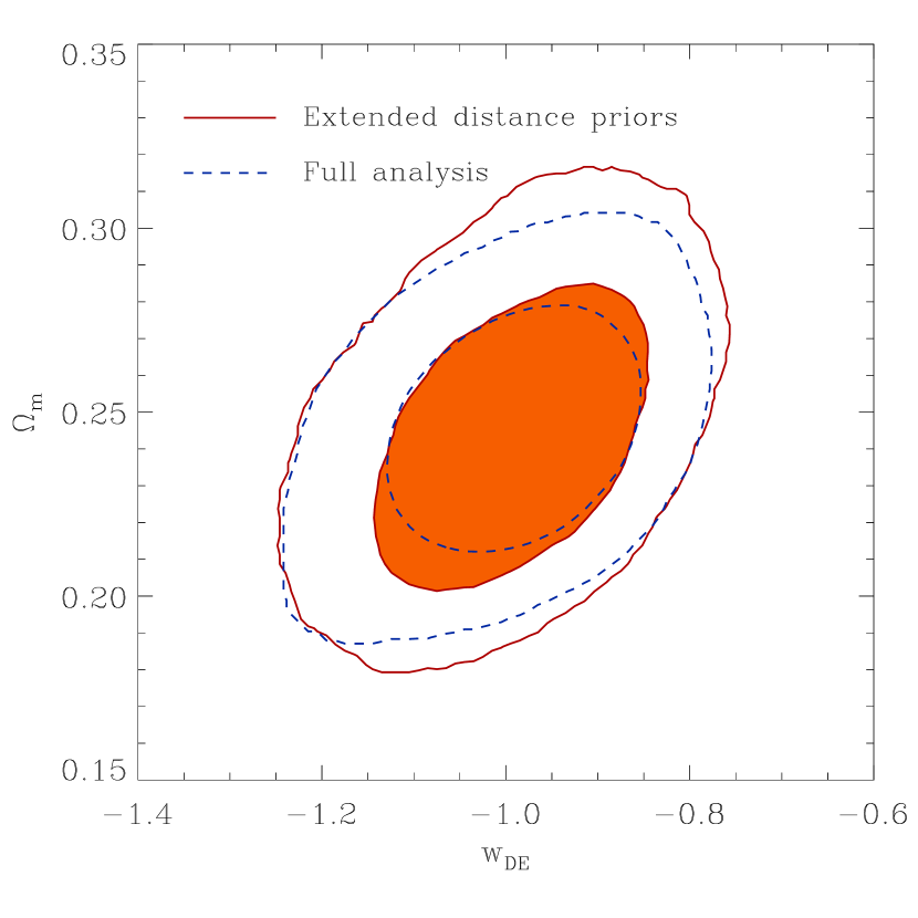
The mean values and covariance matrix of the set of extended distance priors obtained from the combination of CMB information and the shape of the LRG $\xi(s)$ are listed in Tables B1 and B2 of Appendix B. Fig. 16 shows a comparison of the marginalized constraints in the plane $\Omega_{\rm m}-w_{\rm DE}$ for the parameter space of Eq. (7) obtained by using the set of extended distance priors (solid lines) and the ones obtained using the full CMB and $\xi(s)$ data (dashed lines). This shows that this set of constraints contains the most relevant information from the combination of these datasets and can be used to replace them to obtain constraints on cosmological parameters in combination with other cosmological observations like SN data or weak lensing, simplifying and accelerating the required numerical procedure.

7 Conclusions

In this paper, we have applied a new model for the shape of the correlation function at large pair separations to the measurement of LRG clustering from the SDSS made by Cabre & Gaztañaga (2009a). Using a full Monte-Carlo markov chain analysis and combining the LRG measurements with the latest compilations of CMB and SNe data, we have presented a comprehensive set of constraints on cosmological parameters for different combinations of datasets and for different parameter spaces.

Large scale structure measurements and modelling have now reached a level of precision where they provide constraints on cosmological parameters which are competitive with those obtained from other datasets. Using only the LRG correlation function and the measurement of the radial BAO peak, it is possible to determine the dark energy equation of state parameter to $w_{\rm DE}=-1.05^{+0.16}_{-0.15}$. This provides further confirmation of the dark energy scenario, independent of CMB or SN observations.

The availability of several high quality datasets gives us the opportunity to scrutinize the derived constraints and to isolate possible systematic effects in either the observations themselves or the theoretical model used to describe them. In general, different datasets are sensitive to different parameter combinations and the constraints are optimized when datasets are combined. However, in the case in which datasets are responsive to similar parameter combinations, it is important to check that consistent results are obtained before combining the datasets. It would be meaningless to combine two such datasets if a tension existed between the parameters values returned from each one individually.

The tables of parameter constraints given in this paper show that, to first order at least, the “Union” supernova dataset of Kowalski et al. (2008) and the LRG clustering from the SDSS yield very similar constraints on cosmological parameters when analysed in combination with CMB data, for all of the parameter spaces considered. As shown in Section 5.2, the recovered value of the dark energy equation of state in the CMB plus $\xi(s)$ case of $w_{\rm DE}=-0.996\pm 0.090$ shows a remarkable agreement with that obtained from the combination of CMB with the SN data of $w_{\rm DE}=-0.950\pm 0.055$. The consistency of the constraints we obtain from different combinations of datasets is a reassuring validation of our analysis technique.

Percival et al. (2007c), however, found a tension at the 2.4$\sigma$ level between the constraints on $D_{\rm V}(z=0.35)/D_{\rm V}(z=0.20)$ coming from the BAO signal measured from galaxy samples drawn from the 2dFGRS and the SDSS (including a smaller LRG sample than the one considered here), and the SN data from Astier et al. (2006). When folded with the CMB data, this discrepancy leads to different preferred values for the dark energy equation of state, with the SN data preferring $w_{\rm DE}\simeq-1$ and the BAO data pointing to $w_{\rm DE}<-1$ with a significance of 1.4$\sigma$ (see their figures 12 and 13; see also Lazkoz et al. (2008)). Our analysis shows that the LRG clustering and SNe data give consistent constraints on the distance scale $D_{\rm V}(z=0.35)$. The tension reported by Percival et al. (2007c) could result from the BAO signal at $z=0.2$ (which corresponds to the main 2dFGRS and SDSS galaxy samples). This is unlikely to be the answer, however, since the rBAO measurements from Gaztañaga et al. (2008b), which separate the signal at $z=0.24$ and $z=0.43$, also give a consistent answer with $w_{\rm DE}=-0.92\pm 0.15$. The treatment of the BAO feature is quite different in the two analyses. Percival et al. (2007c) effectively take a BAO template generated for a given set of cosmological parameters and then fit this to the measured BAO features for different parameters. Furthermore, the technique of Percival et al. requires a reference spectrum to be defined. Finally, as Percival et al. (2007c) speculate themselves, the problem could lie in the way in which the BAO are damped; these authors assume a fixed damping scale, whereas we treat the damping scale as a parameter.

One criticism that could be levelled at our analysis is the apparent level of agreement between our new theoretical model and the measured LRG clustering. We have shown that the model is remarkably accurate when compared to the correlation function measured for the dark matter or for samples of haloes drawn from N-body simulations (see also Crocce & Scoccimarro, 2008; Sánchez et al., 2008). However, in the case of the observed LRG clustering, the relative height of the BAO feature is greater than predicted by the model. This is illustrated in Fig. 17. This behaviour is not peculiar to the measurement by Cabre & Gaztañaga (2009a). The earlier measurement of LRG clustering by Eisenstein et al. (2005) had a similar form (see also Okumura et al., 2008). A key result from this paper is the dependence of the parameter constraints on the minimum pair separation used in the analysis (Fig. 5). The mean parameter value returned is insensitive to the choice of the minimum pair separation; the only noticeable difference is an increase in the $1\sigma$ range on selected parameters as fewer data points are included. Similar conclusions were reached using a less challenging range of scales by Okumura et al. (2008). This confirms that the information we extract from the overall shape of the correlation function is consistent with that contained in the BAO feature.

Figure 17: Circles with error bars show the redshift space correlation function used in this paper (from Cabre & Gaztañaga, 2009a). The solid line corresponds to our best-fit model within the framework of the basic $\Lambda$CDM parameter space described in Sec. 5.1, while the dashed line includes in addition a systematic K-shift with $K=0.0045$. This shift may originate from unknown systematic effects as described in Sec. 2.1.1. Even though the visual impact seems important, this constant shift (note the bias factor also changes) does not compromise the goodness of fit of our best fitting model or the range of cosmological parameters derived in this paper. Our best fitting model (ie using $K=0$) has a probability of 24 % to be in agreement with the data, as compared with 62 % for the model with $K=0.0045$. Thus there is not a significant improvement on adding a constant shift to the model.

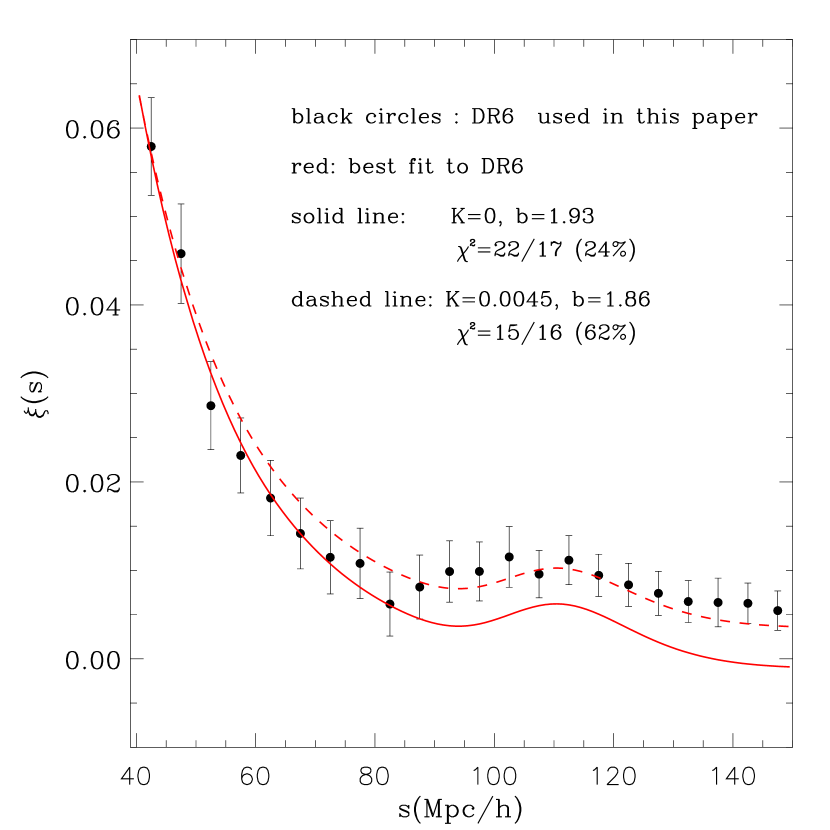
Fig. 17 also considers an extension to our best fitting model which involves allowing for a constant shift in amplitude (Sec 2.1.1). We have tested that the marginalization over a constant additive term has a negligible impact on the cosmological constraints that we derive, which are driven by relative changes in the goodness of fit. However, the addition of this extra nuisance parameter can improve the appearance of the fit and therefore reduce the absolute value of $\chi^{2}$. If we use an absolute $\chi^{2}$ fit with the full covariance matrix, we find a probability of about 25% that our best fitting model describes the measured correlation function (the exact value varies between 20% and 33% depending on which parameters we consider as degrees of freedom). If we allow for a constant systematic shift, as argued in section 2.1.1, the best fit model for the cosmological parameters remains the same, but the probability of the model describing the data improves slightly to 60% in the range $K=0.003-0.006$. This improvement is not significant enough to justify the extra parameter, despite the visual impact of this shift in Fig. 17.

We used the combined information of the CMB measurements and the shape of the LRG $\xi(s)$ to obtain a set of distance priors that combine the most relevant information from these data sets to place constraints on dark energy models and spatial curvature. For this, we expanded the set of distance priors provided by Komatsu et al. (2009) by adding a constraint on the quantity $G(z_{\rm m})$, defined in Eq. (28), which is well constrained by the combination of these datasets (with an error of less than $2\%$). The mean values and covariance matrix of this extended set of distance priors are listed in Tables B1 and B2 of Appendix B. These can be used instead of the combination of CMB and $\xi(s)$ data used in our analysis to obtain constraints on cosmological parameters in combination with other cosmological observations, making the required calculations faster and simpler.

Our analysis shows that current large-scale structure datasets (using the shape of the correlation function at large pair separations, along with the form of the BAO peak) give constraints on the basic cosmological parameters that are competitive with those from the best available SNe datasets. Moreover, possible systematic distortions in the clustering signal have been modelled extensively. The theoretical model applied in this paper has been shown to provide an accurate description of the clustering for the level of error expected in volumes up to two orders of magnitude larger than the current LRG datasets. This bodes well for experiments planned for ten year’s time, which will produce surveys covering volumes in the region of $100h^{-3}{\rm Gpc}^{3}$ (e.g. Cimatti et al., 2008). Nevertheless, it will be prudent to pursue as many approaches as possible to measure dark energy to allow comparisons to be made between the results obtained with different datasets, as carried out in this paper.

Appendix A The theoretical motivation for the model for the shape of $\xi(r)$

In recent years substantial progress has been made in understanding the non-linear gravitational evolution of density fluctuations (Crocce & Scoccimarro, 2006a, 2008; Matarrese & Pietroni, 2007; Matsubara, 2008; Pietroni, 2008; Taruya & Hiramatsu, 2008). Within the theoretical framework of Renormalized Perturbation Theory (RPT), Crocce & Scoccimarro (2006a, b) showed that the evolution of the power spectrum from its initial value in the linear regime, $P_{\rm L}(k)$, can be described as the sum of two contributions

$$P_{\rm NL}(k,z)=P_{\rm L}(k)G^{2}(k,z)+P_{\rm MC}(k,z),$$ (29)

where $G$ is the nonlinear propagator which weights how much power can be directly linked to the linear epoch (e.g. damping the higher BAO harmonics), and $P_{\rm MC}$ represents the new variance generated by mode coupling.

In configuration space, the first term in Eq. (29) leads to a convolution of the linear theory correlation function with a nearly Gaussian kernel (since $G\sim{\rm e}^{-k^{2}}$, see Crocce & Scoccimarro (2006b)), which causes the acoustic peak to broaden and shift to smaller values (Smith et al., 2008; Crocce & Scoccimarro, 2008). In turn, the contribution of the mode-coupling term can be computed to leading order at large pair separation, yielding $\xi_{\rm MC}(r)\propto\xi^{\prime}_{\rm L}(r)\,\xi^{(1)}_{\rm L}(r)$ (Crocce & Scoccimarro, 2008), where $\xi^{\prime}_{\rm L}(r)$ is the first derivative of the linear theory correlation function and $\xi^{(1)}_{\rm L}(r)$ is defined by Eq (11).

In fact, Eq.( 29) is also valid for the nonlinear spectra of density ($\delta$)/velocity divergence ($\theta$) fields, $P_{\delta\theta}$ and $P_{\theta\theta}$,

$$P_{NL,ab}=P_{L}G_{a}G_{b}+P_{MC,ab},$$ (30)

with $a=\delta,\theta$.

To study the impact of redshift distortions and bias we put together the discussion above and the ansatz given in Scoccimarro (2004) (see also Percival & White (2009)):

$$P_{s}({\bf k})={\rm e}^{-k^{2}f^{2}\mu^{2}\sigma_{v}^{2}}\left[b^{2}P_{\delta\delta}+2f\mu^{2}bP_{\delta\theta}+f^{2}\mu^{4}P_{\theta\theta}\right],$$ (31)

where $P_{\delta\delta},P_{\delta\theta}$ and $P_{\theta\theta}$ were introduced above and a local linear bias relation between the density fluctuations in the distribution of galaxies and dark matter is assumed (but with unbiased galaxy velocities). The damping factor in Eq. (31) arises after assuming a Gaussian PDF for the pairwise velocities with rms (if evaluated in the linear regime),

$$\sigma_{v}=\frac{1}{3}\int\frac{P_{\rm L}(q)}{q^{2}}{\rm d}^{3}q.$$ (32)

In Eq. (31) $f$ is the logarithmic derivative of the linear growth rate with respect to the scale factor, $f={\rm d}\,{\rm ln}D/{\rm d}\,{\rm ln}a$, and $\mu=k_{z}/k$ is the cosine of the line-of-sight angle. Note that the small scale redshift space distortions, commonly referred to as “fingers of God” (FOG) due to the elongation of virialised structures, are difficult to model accurately, partly due to the non-Gaussianity of the PDF, which persists even to large scales (Scoccimarro, 2004). In addition, the damping factor depends on galaxy type (or mean halo mass and satellite population)

We are interested in the monopole of the correlation function, i.e. the angle average of the Fourier transform of $P_{s}({\bf k})$ in Eq. (31). Since the time required to evaluate the different power spectra is not well suited to the exploration of large parameter spaces, we would like to motivate a parametric description of the problem.

Crocce & Scoccimarro (2006b) showed that both $G_{\theta}$ and $G_{\delta}$ are of approximately Gaussian form, and with similar smoothing length. Therefore the main contribution to the correlation function at large separations can be modeled, combining Eqs. (31,30), as $\propto\xi_{L}\otimes{\rm e}^{-(k_{\star}r)^{2}}$. The FOG prefactor in Eq.(31) leads to an extra suppression, which is subdominant to that of nonlinear gravity for low redshift data (where $f\sim 0.5$). However, it can be accounted for to some degree by smaller values of $k_{\star}$.

The mode coupling spectra in Eq. (30) do differ at the several $\%$ level (Scoccimarro, 2004), but they all give contributions scaling as $\sim\xi^{\prime}$ (the derivative of the correlation function) in configuration space at large separations. The convolution with the FOG suppression leaves this contribution unaltered as the smoothing length introduced by the FOG is smaller than features present in $\xi^{\prime}$, even at BAO scales.

Therefore we are left with the following parametrization,

$$\xi_{\rm NL}(r)=b^{2}\{\xi_{\rm L}(r)\otimes{\rm e}^{-(k_{\star}r)^{2}}+A_{\rm MC}\,\xi^{\prime}_{\rm L}(r)\,\xi^{(1)}_{\rm L}(r)\},$$ (33)

for the correlation function at large pair separations in redshift space, where $b$ and $A_{\rm MC}$ are nuisance parameters to account for bias and also the enhanced correlation amplitude due to redshift distortions (Kaiser, 1987).

The assumptions behind the model in Eq. (33), one could argue, are over-simplifications, particularly for biased tracers such as LRGs (Zehavi et al. 2005; Blake et al. 2007), or for deeper surveys where a more systematic derivation of redshift distortions may be needed. Nonetheless this form is well motivated given the size of statistical errors in the SDSS-DR6 LRG sample, and based on results from Sec. 3.2 (see also Sánchez et al. (2008)) should be accurate also for future larger surveys.

Appendix B Extended distance priors

Here we list the constraints on the set of extended distance priors described in Section 6. Table B1 lists the mean values and variances of the parameters in this set and Table B2 gives the corresponding covariance matrix. This information can be used to replace the CMB and $\xi(s)$ data in multiparametric analysis since it contains most of the information of the combination of these two datasets. With this simplification, the likelihood of a given cosmological model can be easily computed as $-2\ln{\mathcal{L}}\propto({\mathbf{D}}-{\mathbf{T}})^{\rm t}\textsf{ {{ C}}}^{-1}({\mathbf{D}}-{\mathbf{T}})^{\rm t}$ where ${\mathbf{D}}$ is a vector containing the constraints of Table B1, T contains the corresponding prediction for a given cosmological model and ${\textsf{{C}}}^{-1}$ is the inverse of the covariance matrix of Table B2. This procedure considerably reduces the computing time required to obtain constraints on cosmological parameters compared with the full analysis of the data and can be used in combination with other datasets like weak lensing or the Hubble diagram of type Ia supernovae.

Table 7: The mean values and variances of the parameters in the set of extended distance priors described in Section 6, using the compilation of CMB data in combination with the LRG correlation function.

Parameter	value
$100\omega_{\rm b}$	$2.28\pm 0.55$
$z_{*}$	$1090.12\pm 0.93$
$\ell_{\rm A}(z_{*})$	$301.58\pm 0.67$
$R(z_{*})$	$1.701\pm 0.018$
$G(z_{\rm m})$	$1175\pm 21$

Table 8: The covariance matrix of the parameters in the set of extended distance priors described in Section 6.

	$100\omega_{\rm b}$	$z_{*}$	$\ell_{\rm A}(z_{*})$	$R(z_{*})$	$G(z_{\rm m})$
$100\omega_{\rm b}$	$2.99\times 10^{-7}$	$-4.2030\times 10^{-4}$	$-1.9988\times 10^{-4}$	$-3.4393\times 10^{-6}$	$-1.9978\times 10^{-3}$
$z_{*}$		$8.6812\times 10^{-1}$	0.2557	$1.1999\times 10^{-1}$	3.2355
$\ell_{\rm A}(z_{*})$			0.4558	$3.1265\times 10^{-2}$	1.8247
$R(z_{*})$				$3.1460\times 10^{-4}$	$3.9649\times 10^{-2}$
$G(z_{\rm m})$					$4.3784\times 10^{2}$

References

- Ade et al. (2008) Ade P., ock J., Bowden M., Brown M. L., Cahill G., Carlstrom J. E., Castro P. G., Church, S., 2008, ApJ, 674, 22
- Albretch et al. (2006) Albrecht, A., et al., 2006, preprint astro-ph/0609591
- Angulo et al. (2005) Angulo R. E., Baugh C. M., Frenk C. S., Bower R.G., Jenkins A., Morris S. L., 2005, MNRAS, 362, L25
- Angulo et al. (2008) Angulo R. E., Baugh C. M., Frenk C. S., Lacey C. G., 2008, MNRAS, 383, 755
- Astier et al. (2006) Astier P. et al., 2006, A&A, 447, 31
- Barris et al. (2004) Barris B. J. et al., 2004, ApJ, 602, 571
- Bennet et al. (2003) Bennett C. L. et al., 2003, ApJS, 148, 1
- Blake & Glazebrook (2003) Blake C., Glazebrook K., 2003, ApJ, 594, 665
- Blanton et al. (2005) Blanton M. R. et al., 2005, AJ, 129, 2562
- Bond et al. (1997) Bond J. R., Efstathiou G., Tegmark M., 1997, MNRAS, 291, L33
- Bridle et al. (2003) Bridle S. L., Lahav O., Ostriker J. P., Steinhardt P. J., 2003, Science, 299, 1532
- Cabre & Gaztañaga (2009a) Cabre A., Gaztañaga E., 2009a, MNRAS, 393, 1183, eprint arXiv:0807.2460
- Cabre & Gaztañaga (2009b) Cabre A., Gaztañaga E., 2009b, MNRAS, 396, 1119, eprint arXiv:0807.2461
- Chevallier & Polarski (2001) Chevallier M., Polarski D., 2001, Int. J. Mod. Phys. D., 10, 213
- Cimatti et al. (2008) Cimatti A. et al., 2008, Experimental Astronomy, in press, eprint arXiv:0804.4433
- Cole et al. (2005) Cole S. et al. (The 2dFGRS Team), 2005, MNRAS, 362, 505
- Colless et al. (2001) Colless M. et al. (The 2dFGRS Team), 2001, MNRAS, 328, 1039
- Colless et al. (2003) Colless M. et al. (The 2dFGRS Team), 2003, eprint arXiv:0306581
- Cresswell & Percival (2009) Cresswell J.G., Percival W.J., 2009, MNRAS, 392, 682
- Crocce & Scoccimarro (2006a) Crocce M., Scoccimarro R., 2006a, PRD, 73, 063519
- Crocce & Scoccimarro (2006b) Crocce M., Scoccimarro R., 2006b, PRD, 73, 063520
- Crocce & Scoccimarro (2008) Crocce M., Scoccimarro R., 2008, PRD, 77, 023533
- Crocce et al. (2009) Crocce M., Fosalba P., Castander F, Gaztanaga E., 2009, eprint arXiv:0907.0019
- Desjacques (2008) Desjacques V., 2008, PRD, 78, 103503
- Dunkley et al. (2009) Dunkley J. et al., 2009, ApJS, 180, 306
- Efstathiou & Bond (1999) Efstathiou G., Bond J. R., 1999, MNRAS, 304, 75
- Efstathiou et al. (2002) Efstathiou G. et al., 2002, MNRAS, 330, L29
- Eisenstein & Hu (1998) Eisenstein D. J., Hu W., 1998, ApJ. 496, 605
- Eisenstein & Hu (1999) Eisenstein D. J., Hu W., 1998, ApJ. 511, 5
- Eisenstein et al. (2001) Eisenstein D. J. et al., 2001, AJ, 122, 2267
- Eisenstein et al. (2005) Eisenstein D. J. et al., 2005, ApJ, 633, 560
- Eisenstein et al. (2006) Eisenstein D. J., Seo H., Sirko E., Spergel D. N., 2006, ApJ, 664, 675
- Ellis et al. (2008) Ellis R. S. et al., 2008, ApJ, 674, 51
- Estrada et al. (2009) Estrada J., Sefusatti E., Frieman J. A., 2009, ApJ, 692, 265
- Fang et al. (2008) Fang W., Hu W., Lewis A., 2008, PRD, 78, 087303
- Ferramacho et al. (2009) Ferramacho L. D., Blanchard A., Zolnierowski Y., 2009, A&A, 499, 21
- Fosalba et al. (2008) Fosalba P., Gaztañaga, E., Castander F. J., Manera M., 2008, MNRAS, 391, 435
- Gallagher et al. (2005) Gallagher J. S., Garnavich P. M., Berlind P., Challis P., Jha S., Kirshner R. P., 2005, ApJ, 634, 210
- Gaztañaga et al. (2008a) Gaztanaga E., Cabre A., Castander F., Crocce M., Fosalba P., 2008a, MNRAS in press, eprint arXiv:0807.2448
- Gaztañaga et al. (2008b) Gaztañaga E., Cabre A., Hui L., 2008b, MNRAS in press, eprint arXiv:0807.3551
- Gaztañaga et al. (2008c) Gaztañaga E., Miquel R., Sánchez E., 2008c, eprint arXiv:0808.1921
- Gelman & Rubin (1992) Gelman A., Rubin D., 1992, Stat. Sci., 7, 457
- Gorski et al. (1999) Gorski K. M., Wandelt B. D., Hansen F. K., Hivon E., Banday A. J., 1999, eprint arXiv:9905275
- Glazebrook et al. (2007) Glazebrook K. et al. 2007, ASPC, 379, 72
- Guzik et al. (2007) Guzik J., Bernstein G., Smith R. E., 2007, MNRAS, 375, 1329
- Guy et al. (2005) Guy J., Astier P., Nobili S., Regnault N., Pain R., 2005, A&A, 443, 781
- Hamann et al. (2008) Hamann J., Hannestad S., Melchiorri A., Wong Y. Y. Y., 2008, JCAP, 07, 017
- Hicken et al. (2009) Hicken M., Wood-Vasey W.M., Blondin S., Challis P., Jha S., Kelly P.L., Rest A., Kirshner R.P., 2009, eprint arXiv:0901.4804
- Hinshaw et al. (2003) Hinshaw G. et al., 2003, ApJS, 148, 135
- Hinshaw et al. (2007) Hinshaw G. et al., 2007, ApJS, 170, 288
- Hinshaw et al. (2009) Hinshaw G. et al., 2009, ApJS, 180, 225
- Hogg et al. (2005) Hogg D.W., Eisenstein D.J., Blanton M.R., Bahcall N.A., Brinkmann J., Gunn J.E., Schneider D.P., 2005, ApJ, 624, 54
- Howell et al. (2009) Howell D. A. et al., 2009, ApJ, 691, 661
- Hu & Haiman (2003) Hu W., Haiman Z., 2003, PRD, 68, 063004
- Hu & Jain (2004) Hu W., Jain B., 2004, PRD, 70, 043009
- Huff et al. (2007) Huff E., Schulz A. E., White M., Schlegel D. J., Warren M. S., 2007, Astroparticle Physics, 26, 351
- Huterer & Turner (2001) Huterer D., Turner M.S., 2001, PRD, 64, 123527
- Hütsi (2006) Hütsi G., 2006, A&A, 449, 891
- Hütsi (2007) Hütsi G., 2007, MNRAS, submitted, eprint arXiv:0705.1843
- Jones et al. (2006) Jones W. C. et al., 2006, ApJ, 647, 823
- Kaiser (1987) Kaiser N., 1987, MNRAS, 227, 1
- Komatsu et al. (2009) Komatsu E. et al., 2009, ApJS, 180, 330
- Kowalski et al. (2008) Kowalski M. et al., 2008, ApJ, 686, 749
- Kuo et al. (2007) Kuo C. L. et al., 2007, ApJ, 664, 687
- Lazkoz et al. (2008) Lazkoz R., Nesseris S., Perivolaropoulos L., 2008, JCAP, 07, 012
- Lee et al. (2001) Lee A. T. et al., 2001, ApJ, 561, L1
- Lewis & Bridle (2002) Lewis A., Bridle, S., 2002, PRD, 66, 103511
- Lewis et al. (2000) Lewis A., Challinor A., Lasenby A., 2000, ApJ, 538, 473
- Linder et al. (2003) Linder E. V., 2003, PRL, 90, 091301
- Martinez et al. (2009) Martinez V. J., Arnalte-Mur P., Saar E., de la Cruz P., Pons-Borderia M. J., Paredes S., Fernandez-Soto A., Tempel E., 2009, ApJ, 696L, 93
- Matarrese & Pietroni (2007) Matarrese S., Pietroni M., 2007, JCAP, 06, 026
- Matsubara (2004) Matsubara T., 2004, ApJ, 615, 573
- Matsubara (2008) Matsubara T., 2008, PRD, 77, 063530
- Meiksin et al. (1999) Meiksin A., White M., Peacock J. A., 1999, MNRAS, 304, 851
- Miknaitis et al. (2007) Miknaitis G. et al., 2007, ApJ, 666, 674
- Montroy et al. (2006) Montroy T. E. et al., 2006, ApJ, 647, 813
- Nolta et al. (2009) Nolta M. R. et al., 2009, ApJS, 180, 296
- Norberg et al. (2009) Norberg P., Baugh C. M., Gaztañaga E., Croton D. J., 2009, MNRAS, 396, 19
- Okumura et al. (2008) Okumura T., Matsubara T., Eisenstein D. J., Kayo I., Hikage C., Szalay A. S., Schneider D. P., 2008, ApJ, 676, 889
- Padmanabhan et al. (2007) Padmanabhan N., et al., 2007, MNRAS, 378, 852
- Page et al. (2003) Page L. et al., 2003, ApJS, 148, 233
- Percival et al. (2002) Percival W. J. et al., 2002, MNRAS, 337, 1068
- Percival et al. (2007a) Percival W. J. et al., 2007a, ApJ, 657, 51
- Percival et al. (2007b) Percival W. J. et al., 2007b, ApJ, 657, 645
- Percival et al. (2007c) Percival W.J., Cole S., Eisenstein D. J., Nichol R. C., Peacock J. A., Pope A. C., Szalay A. S., 2007, MNRAS, 381, 1053
- Percival & White (2009) Percival W. J., White M., 2009, MNRAS, 393, 297
- Perlmutter et al. (1999) Perlmutter S. et al., 1999, ApJ, 517, 565
- Piacentini et al. (2006) Piacentini F. et al., 2006, ApJ, 647, 833
- Pietroni (2008) Pietroni M., 2008, JCAP, 10, 036
- Readhead et al. (2004) Readhead A. C. et al., 2004, ApJ, 609, 498
- Reichardt et al. (2009) Reichardt C. L. et al., 2009, ApJ, 694, 1200
- Reid et al. (2008) Reid B. A., Spergel D. N., Bode P., 2008, ApJ, submitted, eprint arXiv:0811.1025
- Riess et al. (1998) Riess A. G. et al., 1998, AJ, 116, 1009
- Riess et al. (2004) Riess A. G. et al., 2004, ApJ, 607, 665
- Riess et al. (2007) Riess A. G. et al., 2007, ApJ, 659, 98
- Ruhl et al. (2003) Ruhl J. E. et al., 2003, ApJ, 599, 786
- Sánchez et al. (2006) Sánchez A. G., Baugh C. M., Percival W. J., Peacock J. A., Padilla N. D., Cole S., Frenk C. S., Norberg P., 2006, MNRAS, 366, 189
- Sánchez & Cole (2008) Sánchez A.G., Cole S., 2008, MNRAS, 385, 830
- Sánchez et al. (2008) Sánchez A.G., Baugh C.M., Angulo R., 2008, MNRAS, 390, 1470
- Scoccimarro (2004) Scoccimarro R., 2004, PRD, 70, 083007
- Seljak et al. (2005) Seljak U. et al., 2005, PRD, 71, 103515
- Seljak et al. (2006) Seljak U., Slosar A., McDonald P., 2006, JCAP, 10, 014
- Seo & Eisenstein (2003) Seo H., Eisenstein D. J., 2003, ApJ, 598, 720
- Seo & Eisenstein (2007) Seo H., Eisenstein D. J., 2007, ApJ, 665, 14
- Seo et al. (2008) Seo H., Siegel E. R., Eisenstein D. J., White M., 2008, ApJ, 686, 13
- Smith et al. (2003) Smith R. E., Peacock J. A., Jenkins A., White, S. D. M., Frenk C. S., Pearce F. R., Thomas P. A., Efstathiou G., Couchman H. M. P., 2008, MNRAS, 341, 1311
- Smith et al. (2007) Smith R. E., Scoccimarro R., Sheth R. K., 2007, PRD, 75, 063512
- Smith et al. (2008) Smith R. E., Scoccimarro R., Sheth R. K., 2008, PRD, 77, 043525
- Spergel et al. (2003) Spergel D. N. et al., 2003, ApJS, 148, 175
- Spergel et al. (2007) Spergel D. N. et al., 2007, ApJS, 170, 377
- Steigman (2007) Steigman G., 2007, on SUSY06: The 14th International Conference on Supersymmetry and the Unification of Fundamental Interactions Edited by Feng J.L., p.40
- Sugiyama (1995) Sugiyama N., 1995, ApJS, 100, 281
- Sullivan et al. (2003) Sullivan M. et al., 2003, MNRAS, 340, 1057
- Swanson et al. (2008) Swanson M.E.C., Tegmark M., Blanton M., Zehavi I., 2008, MNRAS, 385, 1635
- Szapudi (2004) Szapudi I., 2004, ApJ, 614, 51
- Takahasi et al. (2008) Takahashi R. et al., 2008, MNRAS, 389, 1675
- Taruya & Hiramatsu (2008) Taruya A., Hiramatsu T., 2008, ApJ, 674, 617
- Tegmark et al. (1994) Tegmark M., Silk, J., Blanchard A., 1994, ApJ, 420, 484
- Tegmark et al. (2004) Tegmark M. et al., 2004, ApJ 606, 702
- Tegmark et al. (2006) Tegmark M. et al, 2006, PRD, 74, 123507
- Tonry et al. (2003) Tonry J. L. et al., 2003, ApJ, 594, 1
- Wood-Vasey et al. (2007) Wood-Vasey W. M.et al., 2007, ApJ, 666, 694
- Wang (2006) Wang Y., 2006, ApJ, 647, 1
- Wang & Mukherjee (2006) Wang Y., Mukherjee P., 2006, ApJ, 650, 1
- Wood-Vasey et al. (2007) Wood-Vasey M., et al. 2007, ApJ, 666, 694
- Wright (2007) Wright E.L., 2007, ApJ, 664, 633
- Xia et al. (2008) Xia J., Li H., Zhao G., Zhang X., 2008, PRD, 78, 0835524