An analytic model for the bispectrum of galaxies in redshift space
Abstract
We develop an analytic theory for the redshift space bispectrum of dark matter, haloes and galaxies. This is done within the context of the halo model of structure formation, as this allows for the self-consistent inclusion of linear and non-linear redshift space distortions and also for the non-linearity of the halo bias. The model is applicable over a wide range of scales: on the largest scales the predictions reduce to those of the standard perturbation theory (PT); on smaller scales they are determined primarily by the nonlinear virial velocities of galaxies within haloes, and this gives rise to the U-shaped anisotropy in the reduced bispectrum – a finger print of the Finger-Of-God distortions. We then confront the predictions with measurements of the redshift space bispectrum of dark matter from an ensemble of numerical simulations. On very large scales, , we find reasonably good agreement between our Halo Model, PT and the data, to within the errors. On smaller scales, , the measured bispectra differ from the PT at the level of , especially for colinear triangle configurations. The Halo Model predictions improve over PT, but are accurate to no better than . On smaller scales , our model provides a significant improvement over PT, which breaks down. This implies that studies which use the lowest order PT to extract galaxy bias information are not robust on scales . The analytic and simulation results also indicate that there is no observable scale for which the configuration dependence of the reduced bispectrum is constant—hierarchical models for the higher order correlation functions in redshift space are unlikely to be useful. It is hoped that our model will facilitate extraction of information from large-scale structure surveys of the Universe, because different galaxy populations are naturally included into our description.
pacs:
98.80.-kI Introduction
Statistical analyses of the large scale structures observed in galaxy surveys can provide a wealth of information about the cosmological parameters, the underlying mass distribution and the initial conditions of the UniverseTegmark et al. (2004); Cole et al. (2005); Eisenstein et al. (2005); Tegmark et al. (2006); Spergel et al. (2007). Some complex combination of the information is commonly extracted through measurement of the 2-point correlation function, or it’s Fourier space analogue the power spectrum. Since the evolved density field of galaxies is highly non-Gaussian, further complementary information is contained within the higher order clustering statistics Bernardeau et al. (2002); Sefusatti & Scoccimarro (2006). For example, analysis of the large-scale 3-point correlation function, or its Fourier space dual the bispectrum, on large scales, can: test the non-linearity of bias – the way in which an observable tracer distribution samples the unobservable distribution of physical interest Fry & Gaztañaga (1993); Frieman & Gaztañaga (1994); Fry (1994); Sefusatti et al. (2006); constrain our hypothesis of Gaussianity in the initial conditions Fry & Scherrer (1994); Gaztañaga & Fosalba (1998); Scoccimarro et al. (2004); Sefusatti & Komatsu (2007); break degeneracies between parameters, hence allowing improved constraints on the amplitude of the matter power spectrum. In addition, higher order statistics have been highlighted as an important piece of solving the puzzle as to whether the observed accelerated expansion of the Universe is due to Dark Energy physics or a modification to gravity Bernardeau (2004); Shirata et al. (2007); Jain & Zhang (2007); Scoccimarro (2008). On smaller scales these statistics can be most usefully used as a discriminator for the shapes of haloes Smith, Watts & Sheth (2006) – and thus have the potential to constrain the small-scale dark matter physics.
The current state of the art galaxy redshift surveys Saunders et al. (2000); Colless et al. (2001); York et al. (2000); Schneider et al. (2007) have provided large samples of the Universe, and investigators have already carried out some of the tests noted above: 3-point correlation functions have been estimated by Kayo et al. (2004); Jing & Böerner (2004); Wang et al. (2004); Gaztañaga et al. (2005); Nichol et al. (2006); Kulkarni et al. (2007) and bispectra by Scoccimarro et al. (2001); Feldman et al. (2001); Verde et al. (2002); Nishimichi et al. (2006).
The recovery of precise cosmological information from these measurements is not straightforward, owing to the influence of non-linear mass evolution, biasing and redshift space distortions. Current theoretical modeling of the large scale bispectrum rests on results from perturbation theory and non-linear biasing in real (as opposed to redshift) space. In the large scale limit, this gives rise to a simple model Fry & Gaztañaga (1993); Frieman & Gaztañaga (1994); Fry (1994):
| (1) |
where the functions are the reduced bispectra of galaxies and matter, . In the above is the matter bispectrum and the matter power spectrum. The coefficient is the large-scale linear bias parameter and is the first non-linear bias parameter. It is usually assumed that this relation holds in redshift space as well, but that it does not in detail can be seen from the work of Scoccimarro et al. (1999). That it nevertheless appears to be a reasonable working hypothesis was demonstrated by Gaztañaga & Scoccimarro (2005). We shall, hereafter, refer to this model in real and redshift space as PT and PTs, respectively.
There are several reasons why we wish to improve upon PTs. Firstly, it is well known that in redshift space the distortion effects from non-linear structures, such as Finger-of-God (hereafter FOG) distortions, pollute the scales that are usually identified for linear treatment. This can not be accounted for in the perturbation theory in any other way than supposing ‘ad-hoc’ fixes to the model Verde et al. (1998); Scoccimarro et al. (1999). A pragmatist might argue that one may take scales that are sufficiently large that these corrections can be neglected. However, even if we are proficient enough to accurately separate linear from non-linear scales, then we are still faced with loosing a significant amount of information from our data through the restrictions to very large scales. Therefore some means for robustly modeling the FOG effects is clearly of great value as this may allow us to expand the utility of our data set and improve precision.
Secondly, in our study of the large-scale galaxy power spectrum Smith, Scoccimarro & Sheth (2007) we found that there was non-trivial scale dependence arising from non-linear bias and gravitational mode coupling, even on the largest scales currently probed. One may then ask how these properties affect the predicted bispectra.
Thirdly, if we assume that that galaxy velocity field is an unbiased tracer for the velocity field of dark matter, then through studying the higher order clustering statistics in redshift space we have a direct probe of the statistical information of the dynamics of the CDM density field itself Davis & Peebles (1983); Kaiser (1987); Hamilton (1998); Scoccimarro (2004).
In this paper we build a new analytic model for the fully non-linear redshift space bispectrum. We will concentrate on the isotropically averaged (i.e. the monopole) bispectrum, for reasons of simplicity. We work in the context of the halo model Cooray & Sheth (2002), since it naturally affords a means for including linear and non-linear density and velocity information Sheth et al. (2001); White (2001); Seljak (2001); Kang et al. (2002); Smith et al. (2008) and neatly allows for the inclusion of galaxies Benson et al. (2000); Seljak (2000); Peacock & Smith (2000); Scoccimarro et al. (2001); Sheth et al. (2001); Berlind & Weinberg (2002). Furthermore, as was shown in Smith, Scoccimarro & Sheth (2007) the halo model presents a natural framework for understanding the origins of the non-linear scale dependence of bias. However, the limitations of the halo model predictions for precision measurements of the matter power spectrum on large scales have been known for some time now Cooray & Sheth (2002); Smith et al. (2003); Crocce & Scoccimarro (2008); Neyrinck & Szapudi (2007). We will therefore use measurements from numerical simulations, to confirm the validity of our predictions.
The paper breaks up as follows: In Section II we formalize the halo model in redshift space, providing general expressions for the 3-point function and bispectrum. Section III details the necessary components of the model; we pay special attention to the redshift-space clustering of halo centers. Section IV presents the central analytic result of the paper—a calculation of the bispectrum monopole. Some results of evaluating our expressions are presented in Section V. In Section VI we confront our model with measurements from -body simulations. In Section VII we summarize our conclusions.
Although our analysis is general, we shall illustrate our results with specific examples. When necessary, we assume a flat Friedmann-Lemaître-Robertson-Walker (FLRW) cosmological model with energy density at late times dominated by a cosmological constant () and a sea of collisionless cold dark matter particles as the dominant mass density. We set and , where these are the ratios of the energy density in matter and a cosmological constant to the critical density, respectively. We use a linear theory power spectrum generated from cmbfastSeljak & Zaldarriaga (1996), with baryon content of and . The normalization of fluctuations is set through , which is the r.m.s. variance of fluctuations in spheres of radius .
II Halo model in redshift space
II.1 Formalism
In the halo model (see Cooray & Sheth (2002) for a review) the density field is decomposed into a set of dark matter haloes, where a halo is defined to be a region that has undergone gravitational collapse forming a dense virialized ball of cold dark matter (CDM). All statistical quantities of interest are then considered as sums over the halo distribution. Thus to understand the large scale clustering of a distribution of objects, haloes, galaxies or dark matter, we simply require understanding of how the haloes themselves cluster; the different tracer types simply act as weights. In particular, different galaxy populations ‘weight’ haloes differently: the Halo Occupation Distribution (HOD) Benson et al. (2000); Seljak (2000); Peacock & Smith (2000); Scoccimarro et al. (2001); Berlind & Weinberg (2002), specifies how the probability for obtaining galaxies depends on halo mass . To model redshift space statistics, we require additional information about how the large scale velocity field modifies the halo clustering, as well as a model for the distribution function of galaxy velocities within each halo. The halo model in redshift space, at the 2-point level, was developed by White (2001); Seljak (2001); Kang et al. (2002) (hereafter we shall refer to the Halo model in real and redshift space as HM and HMs, respectively). However, some unresolved issues remained with regard to the base formalism. These were resolved by Smith et al. (2008) and our description of 3-point statistics presented here extends these analyses. For completeness some of these details are repeated below. Before continuing, we note that the problem of redshift space distortions in the Halo Model was also recently addressed by Tinker (2007), who used numerical simulations to construct an empirical model for the distribution function of halo pair-wise velocities. Our approach is complimentary to that, since the results for the large-scale halo clustering are derived within the context of the analytic perturbation theory rather than being fit for.
The density field of dark matter, haloes or galaxies may be written as
| (2) |
where refers to the particular choice of weight for the th halo in the sum, i.e. depending on the spectra one wishes to model, and where is the number of galaxies in halo . is the normalized density distribution of objects in redshift space within the th halo. In this paper we shall always assume that , is the mass-normalized density profile of dark matter in redshift space, although our formalism does not rely upon this assumption and may readily be generalized for more complicated mass distributions. At this point the only difference between Eq. (2) and the real space density field, is that we have used to denote comoving spatial positions. However this has the special meaning that Hubble’s law, , is used to infer proper radial positions from recession velocities, where is the proper velocity, is the Hubble parameter and is the proper separation (related to comoving coordinate through ). The notion of redshift space distortions then follow from the fact that objects which form through gravitational instability acquire a local peculiar velocity of their own, and hence the velocity–space mapping in general is non-linear. In this paper we shall work in the plane parallel approximation, where observed structures are located at infinity. Then the mapping is
| (3) |
where the Cartesian components of the position vectors have been written , with . Thus and specify the z-components of the redshift space position vector and the comoving peculiar velocity field , scaled in units of the Hubble parameter, respectively. Note that we take to be negative for convenience.
II.2 Higher order correlations
We may now compute the correlation hierarchy for such a distribution of tracer objects. For a definition of the higher-order clustering statistics in configuration space and their Fourier space dual counterparts we refer to Appendix A. There may also be found useful symmetry properties that we exploit throughout.
Following Scherrer & Bertschinger (1991); Scoccimarro et al. (2001); Cooray & Sheth (2002); Takada & Jain (2003); Smith, Watts & Sheth (2006), the real-space 3-point correlation function () in the halo model, for dark matter, haloes or galaxies, is the sum of three terms: the first represents the case where all three points in space are contained in a single halo; the second is the case where two points are located in one halo and the third is in a separate halo; the third is the case where three points are located in three distinct haloes – we shall refer to these as the 1-, 2- and 3-Halo terms and (, , ). These are written:
| (4) | |||||
| (5) | |||||
| (6) | |||||
| (7) |
where and are the 2- and 3-point correlation functions of halo centers, conditioned on halo masses and where is the halo mass function, which gives the number density of dark matter haloes with masses in the range to .
The inverse Fourier transforms of these 3-point functions are the redshift space bispectra (c.f. Eq. 88). They are written:
| (8) | |||||
| (9) | |||||
| (10) | |||||
| (11) |
where and are the Fourier transforms of the 2- and 3-point halo center correlation functions.
Several advantages are gained from transforming to Fourier space. Firstly, once the integrals over mass are included, requires evaluation of a 12-D integral—the corresponding term is significantly simpler. Indeed, for the case of real space – not redshift space – and for spherical haloes, it is possible to write as the product of 3 2-D integrals. The calculation is slightly more complicated in redshift space but, as we show below, it remains tractable. Thus, to compute the redshift space power spectrum and bispectrum, we require three components: the abundance of dark matter haloes ; a model for the redshift space density profile; and a model for the inter-clustering of dark matter haloes in redshift space. In the following sections we describe our choices for these quantities.
III Ingredients
III.1 Halo abundances and bias factors
The halo mass function plays a central role in the halo model. It has been the subject of much detailed study Press & Schechter (1974); Bond et al. (1991); Sheth & Tormen (1999); Sheth, Mo & Tormen (2001). These studies suggest that, in appropriately scaled units, halo abundances should be approximately independent of cosmology, power spectrum and redshift. These models for also predict that the real-space clustering of halos should be biased relative to that of the dark matter Sheth & Tormen (1999); the way in which real-space halo bias depends on halo mass is related to the shape of . Thus, once the mass function has been specified, the problem of describing halo clustering reduces to one of describing the clustering of the dark matter. Of the many recent parametrizations of , Sheth & Tormen (1999); Jenkins et al. (2001); Warren et al. (2006); Reed et al. (2007), we use that of Sheth & Tormen Sheth & Tormen (1999). Changing to that of Warren et al. Warren et al. (2006) for instance, does not affect the large-scale matter predictions, and changes the results in the non-linear regime by a few percent. Note that for the bispectrum, as was shown by Scoccimarro et al. (2001), a more important issue to be aware of is the finite volume effect, which can significantly change the measured statistics for small volumes. The halo bias factors associated with this mass function are reported in Scoccimarro et al. (2001); we use these in what follows. Smith, Scoccimarro & Sheth (2007) describe other empirical approaches to determining halo bias parameters.
III.2 Density profiles in redshift space
Consider the 6-D phase space density distribution function for dark matter particles within a particular halo, denoted . The density profile and velocity distribution function may be obtained by marginalizing over velocities and positions, respectively:
| (12) |
where is the normalizing mass. The redshift space density profile can be readily obtained from the phase space distribution through transformation to the new random variable , given by our fundamental mapping (Eq. 3). Hence
| (13) | |||||
We now assume that the density distribution of matter within each halo is well described by a spherically symmetric density profile and that the particle orbits are isotropic and independent of position within the halo. Thus, the phase space distribution is separable, i.e. . Since the velocity distribution function is isotropic it may now be written as the product of three independent distributions in the three coordinate directions: ; and we shall hereafter use the notation that . Hence,
| (14) |
Fourier transforming yields the compact expression
| (15) |
where denotes a 2-D wavevector perpendicular to the distortion, and is parallel to it.
This expression shows that the redshift space profile is anisotropic because the spherically symmetric real-space profile has been convolved along the line-of-sight direction with displacements generated by the velocity distribution . That is to say, is the quantity in the model which generates FOG distortions and since it represents virial motions, it is clearly the sort of nonlinear effect that PTs based approaches must model ‘ad hoc’. We also note that if makes the redshift profile substantially anisotropic, then these nonlinear effects may extend farther into the linear regime than one might otherwise have expected.
We caution that this simple model of the halo phase space will almost certainly not be strictly valid, since it clearly neglects many aspects of the more complex physics that we understand to play an important role for the internal dynamics of haloes. 111For example: substructures will produce localized features in the phase space distribution Moore et al. (1999); Klypin et al. (1999); a global asymmetry of the underlying potential, generated through the anisotropic accretion of matter, will distort the velocity structure of the phase space into a 6-D triaxial ellipsoid Jing & Suto (2002 – hereafter JS02), etc. Nevertheless, results from numerical simulations show that the isotropic model is a good approximation, which allows one to write down simple expressions that provide physical insight. 222Kang et al Kang et al. (2002) show that if one considers the ensemble average of the phase space distribution for haloes, then is reasonably well described by a Maxwellian. This result was further corroborated by Kuwabara, Taruya & Suto (2002), who computed for a halo with an NFW density profile Navarro, Frenk & White (1997) by solving the Jeans Equation. They found that it was well approximated by a Maxwellian.
Precise details of the models we employ for the density profile of dark matter and for the 1-Point distribution function of velocities are presented in Appendix B. Note also that owing to these models employing different conventions for the halo mass we must convert between them, and we do this using our procedure from Smith & Watts (2005), see Appendix B.2 for some details.
III.3 Halo center clustering in redshift space
On large scales the success of our analytic model will primarily be determined by its ability to reproduce the large-scale clustering of the halo centers. For this we use the redshift space Halo-PT developed in Smith et al. (2008), which is accurate up to the 1-loop level in perturbation theory. The main result we draw from that work is the idea that the halo density field may be written as perturbation series that involves the standard density PT kernels Bernardeau et al. (2002) and the non-linear bias parameters Fry & Gaztañaga (1993). Explicitly we have the series,
| (16) | |||||
| (17) | |||||
where is the linear theory growth function and is the logarithmic growth rate of the velocity field. The functions are the redshift space Halo-PT kernels symmetrized in all of their arguments and we make explicit their dependencies on halo mass and the scale over which the density field has been smoothed. Kernels up to second order are Hivon et al. (1995); Verde et al. (1998); Scoccimarro et al. (1999):
| (18) | |||||
| (19) | |||||
| (20) | |||||
where we have adopted the short-hand notation:
and where
| (21) | |||||
| (22) |
The quantities are the th order Halo-PT kernels (see Appendix C and Smith, Scoccimarro & Sheth (2007) for complete details). The functions represent the th order Eulerian PT kernels for the divergence of the velocity field Bernardeau et al. (2002). Note that these expressions are almost identical to the redshift space PT kernels derived by Scoccimarro et al. (1999); Verde et al. (1998), however they differ in some subtle ways: one, we have explicitly included their dependence on the smoothing filter , which is needed to facilitate the Taylor expansion; and two, we are applying this in the context of haloes and not galaxies and so they depend on the non-linear halo bias parameters , instead of the nonlinear galaxy bias parameters (see discussion in Section III.1). Note that we have also included , since this does not have to be zero, although we will take it to be so for all our later analysis.
Following standard methods for calculating polyspectra, we find that the halo center bispectrum, , up to fourth order in redshift space Halo-PT, is
| (23) | |||||
Inserting our expressions for the redshift space Halo-PT kernels, Eqs (18–20), in to the above expression, reveals:
| (24) | |||||
where and where . As in our real space work on the power spectrum, we are now faced with the situation that we have solved for the bispectrum of halo centers filtered on scale , and in fact we would like to recover the unfiltered bispectrum. As in Smith, Scoccimarro & Sheth (2007), we take the following ansatz: the filtering of the spectra can be reversed through the following operation:
| (25) |
and this explains the form of the left-hand-side of Eq. (24). An alternative approach to the filtering issue for the power spectrum and bispectrum was proposed by Mc Donald (2006), we shall leave the solution of this problem for future consideration.
With these ingredients prepared, we are now in full possession of a complete description of the bispectrum of galaxies, haloes and dark matter in the halo model and in the presence of a local, non-linear scale dependent bias. In the next section we develop these equations further.
IV The Bispectrum Monopole
IV.1 Euler angle averages
The redshift space bispectrum is an anisotropic function on the sphere that depends on 5 variables. The first three are the triangle configuration, and the other two specify its orientation with respect to the z-axis. However it is common practice to measure this quantity averaged over all possible orientations of the coordinate frame. Thus to compare with this isotropized observable, we shall now derive the isotropized form for the halo model, which we shall denote . Interestingly, the following approach is identical to that which one performs for the triaxial halo model in real space Smith & Watts (2005); Smith, Watts & Sheth (2006), since on small scales, one may effectively think of transforming to redshift space as simply transforming a set of spherical haloes into a set of prolate ellipsoids whose semi-major axes all point along the line-of-sight. Of course, the real situation is more complex, since the halo centers are also distorted according to the halo velocity projected along the line-of-sight, but nevertheless we may borrow some mathematical machinery from the triaxial halo analysis.
The isotropic function is thus,
| (26) | |||||
where is the rotation matrix for the components of the basis vectors. is parametrized by three position or Euler angles, (,,) and these are the rotation angles (see Appendix D for the explicit form of the matrix we use). Note that we assign uniform probability on the sphere to each triple of angles.
The following considerations simplify this expression considerably. Firstly, in the PT expressions for , each term depends on either the angle between two k-vectors or the projection of each vector along the -axis. In the first case, the use of matrix notation shows that
| (27) | |||||
this is the well-known result that scalar products are invariant under rotations of the coordinate basis functions. In the second case, the projection of each rotated vector onto the line of sight direction (or z-axis) can be written
| (28) | |||||
Thus, we see that the resultant function must be invariant under the rotation, and hence this integral may be computed trivially. Finally, because our final quantity must be independent of the initial locations of the -vector triple, we may without loss of generality choose these locations to be as convenient as possible. Therefore, we let the initial vector lie along the polar-axis and constrain and to lie in the – plane: i.e.
| (29) |
where the last equality uses the closure condition: . Thus, the -vectors rotated into the new basis and dotted with the -direction are now written:
| (30) |
The parameters are simply related to the cosines of the -vectors along the -axis:
| (31) |
where .
We may now apply the above operation directly to our expressions for the anisotropic bispectrum (Eqs 9–11). On inserting the into each instance of in the density profiles (Eq. 15) and the halo center power spectra and bispectrum (Eqs 114 & 24), we find that the 1-, 2- and 3-Halo terms for the bispectrum monopole become
| (32) |
| (33) | |||||
| (34) | |||||
The only variables that depend on the Euler angles and are and . Each term requires evaluation of no more than a 4-D embedded integral: two integrals for the Euler angles, one for the mass, and one for the Fourier transform of the density profile. Note that for simplicity, we have kept only the leading order contribution to the the 2-Halo term. Technically this should be taken up to the 1-Loop level to be consistent with the bispectrum which is 4th order in . However, this issue is beyond the scope of the current paper and will be addressed in Smith et al. (2008).
IV.2 Computational considerations
Our expressions for the bispectrum as presented above are complete. However some calculational effort is still required before we may attempt a practical implementation on the computer. We now present some simplifications.
We begin by defining some convenient notation: Let and denote the following integrals:
| (35) | |||||
| (36) | |||||
The first integral generalizes the halo bias weighting scheme applied to the density field for the situation where -points are within a single halo. The second integral generalizes the weighting scheme to the similar situation for the halo velocity field. This notation has some similarities with that of Seljak (2001), but is different in the way in which the velocity field is treated – recall that the velocity field has been assumed to be unbiased.
In this notation we may re-write the 2- and 3-Halo terms in the bispectrum; the 1-Halo term requires no simplification. Through rearrangement of the mass integrals and expansion of the halo center power spectrum through substitution of the appropriate kernels, we find that the 2-Halo term can now be written
| (37) | |||||
The 3-Halo term is significantly more complex, owing to the halo center bispectrum being the product of two first order kernels and one second order kernel. Nevertheless, we may again isolate the integrals over mass and use the functions to obtain
| (38) | |||||
where we have defined the following useful quantities:
| (39) | |||||
| (40) | |||||
| (41) | |||||
| (42) |
and
| (43) |
IV.3 The large-scale limit
Next we consider the redshift space bispectrum in the very large scale limit, as this should asymptotically reduce to the standard PT expressions for the bispectrum, modulo discreteness corrections for the point process associated with the halo field. However, let us first examine the large-scale limit of Eqs (35) and (36). On letting , the density profile terms become , the window function becomes , and so
| (44) |
where , with , being the total number density of haloes in the required mass range. When we write these functions more simply as: the average non-linear bias parameter for the tracer particles, , and the logarithmic growth factor for the linear velocity field .
The bispectrum in the large-scale limit can now be computed directly. The 1-Halo term is trivially obtained, and the 2- and 3-Halo terms can be developed through replacing the functions in the general expressions (37) and (38), for their large scale forms (44). After some algebraic manipulation we arrive at the result
| (45) | |||||
where the large scale PT bispectrum monopole in redshift space is given by
| (46) | |||||
this is equivalent to that found by Verde et al. (1998); Scoccimarro et al. (1999). We also defined the 1– and 2–Halo ‘effective’ number densities to be:
| (47) |
| (48) | |||||
Our final expression for the large-scale limit (Eq. 45) is similar to the standard theoretical expectation for the bispectrum recovered from a Poisson point process sampling of a continuous field (c.f. Section 43 in Peebles (1980)). However, the halo model effective shot-noise terms (the last two terms on the right hand side of Eq. 45), are very different from the standard form, which would simply have e.g. . These effective number densities, Eqs (47) and (48), represent the fact that in the halo model we assume that dark matter haloes are Poisson sampled into the density field and that the tracer particles are injected into these haloes, and so simply act as different weights. The issue of sampling tracer particles into the density field has some important implications for how one should extract information from galaxy surveys. We shall reserve this investigation for future work.
In Appendix F we present a short discussion of how these shot noise corrections can impact the reduced bispectrum. The main results are as follows: For standard shot noise, and in the low-sampling limit there is no configuration dependence and , sub-script d denotes discrete. For the case where shot noise is sub-dominant, the is reduced relative to the continuum limit for all configurations. In the halo model, and in the low sampling limit, again there is no configuration dependence and . For the case of sub-dominant shot noise, is not necessarily smaller than the continuum limit case. In Sec. VI we show some tentative evidence for these effects in the measurements from our numerical simulations.
Before continuing, it should also be noted that on setting , one may recover the 1-Loop PT bispectrum in real space for a set of biased tracer particles .
IV.4 The small-scale limit and hierarchical models
On small scales, the bispectrum is dominated by the 1-Halo term, given by Eq. (32). Our understanding of its behavior in this limit can be guided by considering the case where all haloes are of the same mass. In this situation we have and . Applying these conditions to Eq. (32), we have:
| (49) | |||||
We may follow this same procedure for the power spectrum (see Eq. 112) and so construct the reduced bispectrum, whence
| (50) |
where is given by Eq. (119). Notice that this expression no longer depends on the weights or number densities of tracers , but simply the real space profile and the 1-PT velocity profile. If the density and velocity profiles were mass independent, then Eq. (50) would predict the same configuration dependence for all haloes. However, for realistic redshift space profiles, this is not the case (see Appendix B). Thus, if the halo model is a good description for small scale clustering, then the hierarchical model is unlikely to be correct in real or redshift space, and we may generally extend this statement to any tracers of the density field. Finally, and somewhat interestingly, notice that if the ratio is mass independent, then the configuration dependence of the bispectrum becomes universal, modulo an amplitude off-set.
IV.5 The White-Seljak Approximation
The White-Seljak approximation (hereafter WS) is the supposition that haloes are randomly oriented relative to each other so that in computing the monopole of the bispectrum, orientation averages can be taken separately over each individual halo and over the large scale orientation of the halo relative to each other White (2001); Seljak (2001). In the triaxial halo model, Smith & Watts (2005) showed that the overall contribution from halo alignment to the matter power spectrum was negligible. Thus we may similarly assume that on large-scales the 2– and 3–Halo terms will not be sensitive to the orientation of the FOGs – and this allows us to use the isotropic redshift space density profiles instead of the anisotropic profiles. However, since the bispectrum is more sensitive than the power spectrum to the shapes of structure, we shall be a little more cautious, and demonstrate the validity of this approximation in Section V.1.
In the WS approximation we therefore take,
| (51) |
and with similar expressions for the functions. On replacement of these terms into Eq. (37) we find that the 2-Halo term simplifies to:
| (52) | |||||
Similarly, on applying the WS approximation to Eq. (38), the 3-Halo term reduces to:
| (53) | |||||
where
| (54) | |||||
This completes our analytic investigation. In the next sections we shall provide numerical evaluation of our expressions for the bispectrum.
V Analytic results
V.1 Testing the WS approximation
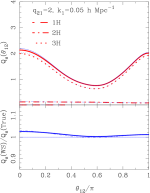
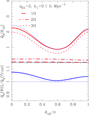
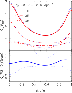
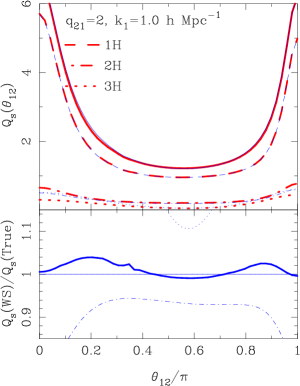
Figure 1 compares the predictions for the reduced redshift space matter bispectrum (Eqs (32), (37), and (38)) with the WS approximate expressions Eqs (32), (52), (53). The four panels show -space triangles with and with .
On very large scales (top left panel), , the predictions are dominated by the 3-Halo term, and the approximate expressions (thin blue lines) are in almost perfect agreement with the exact Halo Model predictions (thick red lines), with deviations across different configurations. This is to be expected following our derivation of the bispectrum in the large-scale limit, c.f. Eq. (45); i.e., there is no dependence on the halo profiles and so the WS approximation does not play a role here. On slightly smaller scales (top right panel) , small but significant departures are found at the level of . It can be seen that these are entirely due to deviations in the 3-Halo term – the order in which we spherically average the profiles is now important. However, on still smaller scales (bottom left panel) , whilst the discrepancy between the approximate and exact 3-Halo term becomes larger, the 1- and 2-Halo terms begin to dominate and so the difference in the total appears . Finally, on the smallest scales considered, the 1-Halo term comes to fully dominate and since no approximation is made here the results are in good agreement, .
For a given scale, the largest deviations typically appear for the case of colinear triangles, i.e. where all three -vectors are co-linear. This leads us to suppose that the equilateral bispectrum as a function of scale will show agreement at the level of across a wide range of scales under this approximation. Since current observational measurements of the bispectrum on large scales have sample and cosmic variance errors of the order on scales , going down to several percent at , we anticipate that, at least for current data, the WS approximation should be useful. We highlight again that the main advantage of this approximation is the increased speed with which one can compute the bispectrum: the and functions are only evaluated once for a particular configuration, as opposed to thousands of times. However, in all that follows we shall only show results for the exact evaluation (no WS approximation) of our redshift space Halo Model.
V.2 Comparison with perturbation theory
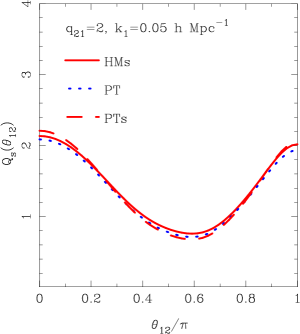
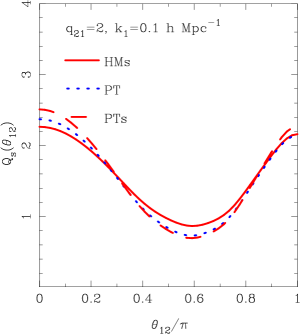
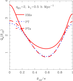
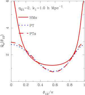
Figure 2 compares the analytic predictions for the reduced bispectrum from our model with corresponding results from PT. The four panels show again -space triangles with with and for the same scales as presented in Fig. 1. The solid (red) lines in each panel show our HMs predictions (recall HMs means Halo Model in redshift space) in the WS approximation. The (red) dash lines show the PTs predictions, as given by our Eq. (46). The (blue) dotted lines correspond to real space PT predictions.
On the largest scales (top-left panel), the HMs and PT results match almost perfectly: the configuration dependence shows excess signal for colinear triangles, indicating that on these very large scales non-linearity induces structures that are, on average, more filamentary than spherical Scoccimarro et al. (1998, 1999) (in this diagram spherical perturbations are best probed by isosceles triangles, ). However, we notice that there is a small deviation for the situation where the and vectors are aligned. This owes to the fact that the 1- and 2-Halo terms are non-vanishing as , and as discussed in Section IV.3, this gives rise to an ‘effective shot-noise’ like behavior. A discussion of why co-linear – triangles (i.e. ) are more preferentially affected is given in Appendix F). It should also be noted that unlike for the case of standard shot noise, for configurations close to isosceles triangles.
On slightly smaller scales , both the PT and PTs predictions show a small increase in configuration dependence, with the PTs having slightly more signal for colinear triangles than PT. The HMs predictions are in qualitative agreement with PT. However, the flattening off seen in the previous panel is now much more apparent. Recalling the corresponding panel in Fig. 1, it can be seen that this is attributed to the rapidly rising 1- and 2-Halo terms.
On smaller scales still , the PT and PTs predictions continue their previous trends, exhibiting a slightly increased configuration dependence. However, the HMs predictions are quite different, having a very strong -shaped configuration dependence. This owes to the 1- and 2-Halo terms becoming dominant.
On the smallest scales considered , the HMs predictions show a dramatic configuration dependence, with a very strong signal for colinear triangles and a broad plateau for triangle shapes around isosceles configurations – this is the ‘U-shape’, which was first noted in the bispectrum by Scoccimarro et al. (1999) and in the 3-point correlation function by Gaztañaga & Scoccimarro (2005). Recalling Fig. 1 (bottom left panel), we see here that the prediction is completely dominated by the 1-Halo term, and so this U-shape feature is simply an imprint of the halo shape in redshift space – the FOG. This result constitutes a more direct demonstration of the discussion from Section IV.4, that hierarchical models are unlikely to be a good description for the higher order clustering statistics.
In this section we have shown from purely theoretical considerations, that to use the galaxy bispectrum on large scales as a precise tool for cosmology, one needs to understand exactly how to include the FOG effect into the modeling and also how to include non-trivial discreteness effects of matter. In the next section we confront the model with results from numerical simulations.
VI Comparison with numerical simulations
VI.1 Numerical simulations
In order to test our redshift space bispectrum we generated an ensemble of 8 LCDM simulations, these were identical in every way, except that for each simulation different random realizations of the initial Fourier modes were drawn. The cosmological parameters for the ensemble were selected to be in broad agreement with the WMAP best fit model Spergel et al. (2007): , , , and . We used the cmbfast Seljak & Zaldarriaga (1996) code to generate the linear theory transfer function, and we adopted the standard parameter choices, and took the transfer function output redshift to be at . The initial conditions for each simulation were then laid down at using the publicly available 2LPT initial conditions generator Scoccimarro (1998); Crocce et al. (2006). Subsequent gravitational evolution of the equations of motion was then performed using the publicly available Gadget2 code Springel (2005). Each simulation was run with particles in a comoving volume of length and with a comoving force softening set to 70 kpc. The simulations were performed using a 4-way dual core Opteron processor system, and each ran to completion in roughly 1800 timesteps from redshift to and this translates to 2 days of wall clock time.
VI.2 Estimating the power spectrum
Before comparing our analytic model with the bispectra estimates from the simulations, it is instructive to compute the real and redshift space power spectra of the outputs of the ensemble.
The density Fourier modes are estimated using the conventional Fast Fourier Transform (FFT) method: the dark matter particles were assigned to a regular cubical grid using the ‘Cloud-In-Cell’ (CIC) scheme Hockney & Eastwood (1981). The FFT of the gridded density field was then computed using the publicly available FFTW routines FFTW . Each resulting Fourier mode was then corrected for the convolution with the mesh by dividing out the Fourier transform of the mass-assignment window function. For the CIC algorithm this corresponds to the following operation:
| (55) |
where
| (56) |
where sub-script d and g denote discrete and grid quantities, and where is the Nyquist frequency of the mesh and is the number of grid cells.
The power spectra of the discrete particles on scale are then estimated by performing the following sums,
| (57) |
where is the number of Fourier modes in a spherical shell in -space of thickness . Note that the mode-by-mode correction differs from the analysis of Smith et al. (2003); Jing (2005) where the correction for charge assignment was performed by computing the spherically averaged window and dividing it out. Mode-by-mode correction for the power spectrum was also performed in Scoccimarro et al. (1998); Smith, Scoccimarro & Sheth (2007).
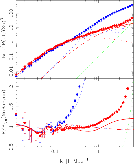
Figure 3 shows the mean and 1- errors for the power spectra of dark matter particles in both real and redshift space. The errors are computed directly from the 8 realizations. The spectra were computed using a FFT and we show all frequencies up to the Nyquist frequency – the highest -modes show signs of increased power from both Poison shot noise (triple dot-dash green line) and the aliasing of power from smaller scales. We note that on the largest scales probed, the power spectra show a sequence of wiggles, these are the well known Baryonic Acoustic Oscillations (BAO) that have been discussed much in recent times Eisenstein & Hu (1998); Meiskin, White & Peacock (1999); Eisenstein et al. (2005); Smith, Scoccimarro & Sheth (2007, 2008) – we shall not discuss these in this paper. The solid lines show the total halo model predictions in real (blue lines) and redshift space (red lines). We see that, whilst the real space model does reasonably well, with an accuracy of the order , the redshift space predictions fare less well, especially for scales . Here the model systematically underpredicts the data by roughly .
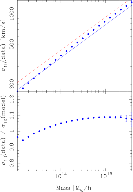
These predictions were very sensitive to how we modeled the FOG effects, i.e. the 1D velocity dispersion of particles within haloes . Originally, we had simply used Eq. (103) with , however in this case the predictions were particularly poor. We therefore investigated relation in our simulations more closely. Using a standard Friends-of-Friends (FoF) algorithm with link length , we located all haloes with . The 1D Velocity dispersions were then estimated for each halo and binned as a function of mass. We found that overpredicted the measured values by . Fitting on it was found that provided a better fit to the data, but it was not perfect, it having an accuracy no better than (see Fig. 6). As can be seen from the figure using does not generate the correct power spectrum.
A possible reason for this discrepancy could be that the 2-Halo term in the redshift space power spectrum only includes linear halo motions – non-linear terms do contribute to this term (see Sheth et al. (2001); Scoccimarro (2004); Smith, Scoccimarro & Sheth (2008)) and inclusion of these non-linear corrections may help alleviate this problem. Another, is that the concentration–mass relation, which is vital for getting the correct normalization of the halo density profiles, may not be sufficiently accurate. Indeed we note a small discrepancy between the real space measurements and Halo Model predictions. Recent improvements on this relation by Neto et al. (2007) may help to alleviate this problem. Also, we have neglected the scatter in the concentration parameter, and it is well known that this can change the predictions by a few tens of percent in the nonlinear regime Hu & Cooray (2001). Additionally, there is the issue of halo triaxiality Smith & Watts (2005); Smith, Watts & Sheth (2006). We shall not pursue these subtle corrections here, since our purpose is to simply present the theoretical framework and show that it gives reasonable agreement with the simulation data.
VI.3 Estimating the bispectrum
Our estimator for the bin and spherical averaged bispectrum was developed following the work of Scoccimarro et al. (1998), but with some changes. Our estimator can be written:
| (58) | |||||
where
| (59) |
A practical implementation of this estimator involves computing the following sum
| (60) |
where is an integer vector from the -space origin to a mesh point and so labels the modes, and where represents the number of independent momentum conserving -vector triangles in the shells and . In the above we take only the real part of the product of the three Fourier modes, owing to the reality of the bispectrum (see Eq. 91). Note that when computing the sums over -space triangles we randomly sample modes from the set of all possible triangles. Typically we limit the computations to modes per shell (i.e. triangles). This method gives a sufficient number of independent -space triangles for a high accuracy estimate, whilst keeping code execution times tolerable.
To accurately estimate we are also required to estimate the combination . There are several approaches to achieving this: one, we could simply estimate the power spectrum as in Eq. (57) and then construct from this; alternatively one can compute an estimate of using only those same modes that are used to estimate . We adopt this latter approach since expect that it will reduce sample variance. Along with our estimates for , we also therefore accumulate
| (61) | |||||
| (62) | |||||
| (63) |
We draw close attention to the fact that these estimates for the power spectra , and are not the same as in Eq. (57): in the above case we average over all -space triangles that are used and not just the unique modes. We have also made it explicitly clear that the estimates for and do not change with , but that does. Following this procedure helps to reduce cosmic variance. We also note the following pitfall: had we estimated for each -space triangle and then averaged these estimates over all triangles, i.e. taken , then we would have been angle averaging products of power spectra. In real space, where is an isotropic function on the sphere, this makes no difference, however in redshift space, where is anisotropic, this approach would be incorrect and no U-shape would be seen in .
In order to correct and for discreteness we also estimate the shot noise terms as Peebles (1980):
| (64) | |||||
| (65) | |||||
| (66) |
Estimates of the shot noise corrected continuous spectra are then arrived at through the following set of operations:
| (67) | |||||
| (68) | |||||
| (69) | |||||
| (70) |
In our measurements we shall show both spectra with and without the shot noise corrections.
Lastly, as a consistency check, we also estimate the imaginary bispectrum, which is given by Eq. (60) only now we take the imaginary piece of the product. Thus, if our estimate is correct, then this quantity should on average be zero. However, as the number of independent triangles becomes small the imaginary piece may become non-zero due to statistical fluctuations.
VI.4 Bispectrum results
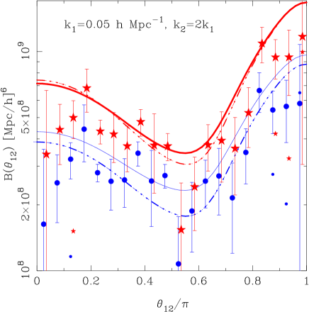
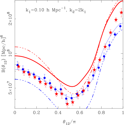
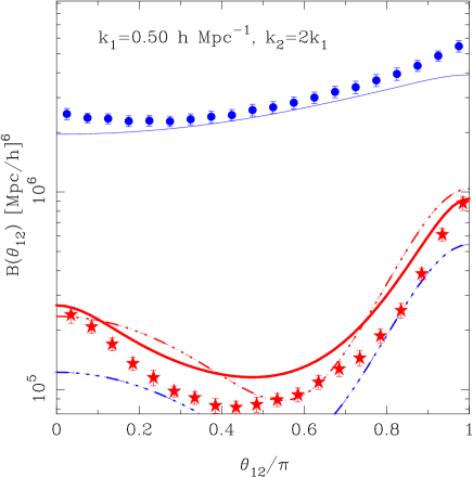
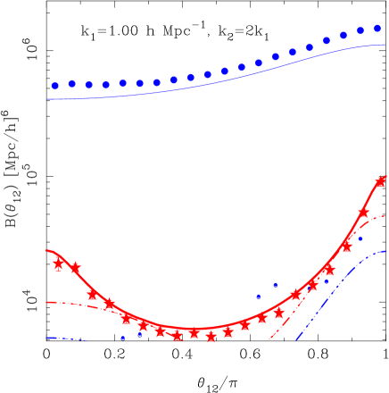
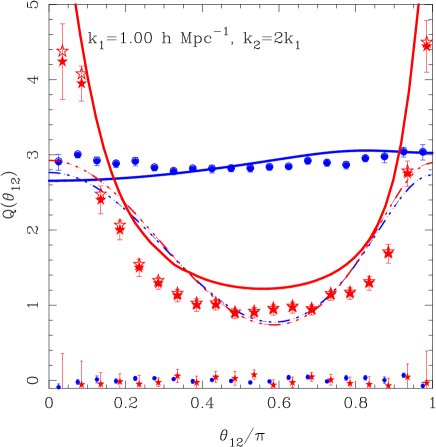
Figure 4 shows the mean and the 1- errors on the mean (i.e. we divide the standard error bars by ) for the configuration dependence of the bispectrum in both real and redshift space for the 8 LCDM simulations. The four panels show results for -space triangles with and and thin (blue) and thick (red) lines distinguish between real and redshift space quantities.
Considering the largest scales (), we see that the ensemble estimate is rather noisy, this owes to the large sample variance on these scales. Nevertheless, it can be discerned that the redshift space (large solid stars) estimate has a slightly higher amplitude than the real space (solid points) estimate. We also note that there are a few bins that give a significant non-zero contribution to the imaginary bispectra. We attribute this to the large sample variance errors, but in the main these points are below the true signal. In all cases the results for the bispectra appear to be consistent with the PT and HM predictions, to within the errors. To say anything more definite on these scales will require much larger simulation volumes, and we shall defer this question for future study.
On intermediate scales (), the estimates for the real and redshift space spectra are much more significant, the errors being well defined. This is supported by the fact that the imaginary spectra have amplitudes that are now too small to be plotted. It can be seen that the results have a strong dependence as a function of triangle configuration. On comparing with the PT and PTs, we see that on these scales PT under-predicts the measured quantity by roughly , whereas PTs overpredicts the amplitude by a similar amount. Considering the predictions of the HM and HMs, it is clear that in real space the model is a significant improvement over PT; whereas in redshift space, whilst the configuration dependence appears to have been slightly improved, the amplitude is still too large.
On smaller scales (), we see that the estimates of the spectra are of even higher signal-to-noise and that they form tight-loci across the configuration. Again the imaginary bispectra are insignificant. It may be noticed that there is a large difference between the real space PT and the simulation estimate – almost two orders of magnitude, this is due to the fact that and the power spectrum is significantly larger than linear. However, this dramatic change in the measured bispectrum is captured relatively well by the HM, which underpredicts the result by only . Turning to the redshift space results, we are surprised to see that the PTs is of the same amplitude and has somewhat similar configuration dependence as the estimate. This agreement seems coincidental, given the poor agreement in real space. In reality the true dynamics on these scales must already be very non-linear. Lastly, we draw attention to the fact that our HMs result is in excellent agreement with the simulation data.
Examining scales on the order of the virial radii for clusters (), we see again that the estimates are of very high significance. Again, the HMs predictions are in excellent agreement. This essentially vindicates our form for the 1-Halo term, and means that the configuration dependence is very much governed by the FOG distortions.
VI.5 Reduced bispectrum results
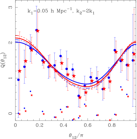
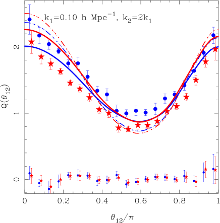
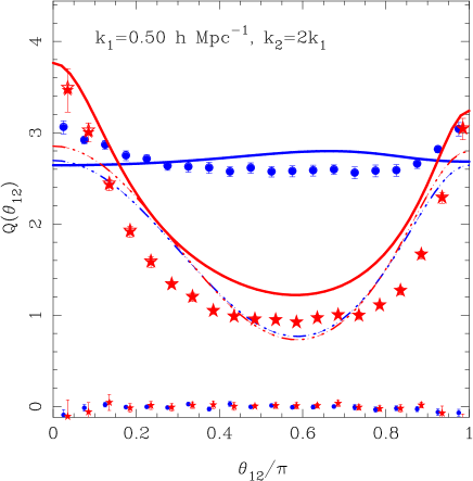
Figure 5 shows similar results as in Fig. 4 but for the configuration dependence of the reduced bispectrum, . Again errors are shown on the mean of .
On the largest scales probed, (), the estimates are noisy, but there is evidence for an excess of signal for co-linear triangles – meaning that on average structures are more filamentary than spherical on the largest scales Scoccimarro et al. (1998, 1999). Also, the data appear to be scattered about the theoretical predictions, with all models being equally good fits to the data.
Considering intermediate scales (), the estimates are much more significant and possess well defined configuration dependencies – both showing an excess of signal for colinear triangles. However, the real space bispectrum appears to be in excess of the redshift space quantity. This is in contrast to the PT and PTs predictions which, whilst qualitatively capture the overall shape, predict the reverse trend, the results being discrepant by roughly . This problem is also mirrored in the HM and HMs predictions, but the flatter configuration dependence of the data is better captured by the Halo Model. As was discussed in Sec. IV.3, this flattening can be attributed to the impact of the 1- and 2-Halo terms acting as effective shot noise contributions. The amplitude offsets still require explanation, and we refer to our discussion of Sec. VI.2 for some possible remedies, but to that list we may now add the need for loop corrections to the tree-level bispectra. As was shown in Scoccimarro et al. (1998), in real space the 1-Loop corrections are significant on these large scales.
On smaller scales (), we see that, as was noted in Fig. 5, the real space measurements have increased in amplitude and have become much flatter across the configuration – the HM predictions agree rather well with this result. This implies that the statistic is already in the fully non-linear regime, since the 1- and 2-Halo terms are dominating the signal here. There is very little relation between standard PT to the measurements, as expected. Turning to the redshift space estimates, it can be seen that the configuration dependence displays a reasonably strong -shape. The PTs predictions do not describe this shape very well, but are not as discrepant as in real space. However, HMs predictions capture the form of the configuration dependence exceptionally well, but are offset by .
Considering the scales associated with the virial radii of clusters (), we see that the estimates in real space are surprisingly unchanged and that the HM still provides a very good description of the data. For the redshift space estimates, we find that there is now a very strong -shape configuration dependence, in full agreement with the results from Scoccimarro et al. (1999). Again, the HMs predictions capture this result remarkably well, although there is a small amplitude offset. It is believed that this may be mitigated by implementing the improvements discussed in Sec. VI.4 and Sec. VI.2.
We also note that the small discrepancies between the real space HM predictions and the simulations, are entirely consistent with the work of Smith, Watts & Sheth (2006) – in reality haloes are triaxial rather than spherical, and this shows up as a characteristic increase in signal for colinear triangles and a suppression for isosceles configurations.
VI.6 Code comparison
Owing to the algorithmic differences between the bispectrum estimation procedure presented in Section VI.3 and that presented in Scoccimarro (2000), we decided to compare the results obtained from these two approaches. Besides providing an important cross-check, this also enables us to examine how accurately the two codes are recovering . Overall we found very good agreement between both methods, and full results are presented in Appendix G.
VII Conclusions
In this paper, we have provided a new analytic model for the redshift space bispectrum of dark matter, haloes and galaxies in the plane parallel approximation for the redshift space distortion. On large scales, the model predictions have a direct correspondence to the non-linear perturbation theory and on small scales, the predictions are entirely governed by the phase space density of galaxies/dark matter internal to the haloes. This is the first time that the information from bulk flows and virial motions have been naturally incorporated into an analytic model for the higher-order clustering statistics in redshift space.
In our analytic model, the bispectrum is represented as a sum over three terms; these correspond to all of the possible distinct arrangements of three points in three haloes, and we referred to these as the 1-, 2- and 3-Halo terms. A practical evaluation of the monopole of the bispectrum (a direct observable), with realistic models for halo profiles, abundance and clustering, required the execution of a set of 4-D numerical integrals. For the terms that involved large-scale correlations (2- and 3-Halo terms) it was shown that these expressions could be easily modularized, and so are best computed in parallel. The 1-Halo term must be integrated with an efficient higher-dimensional integrator.
It was shown that the large-scale predictions in the model, which are governed by the 2- and 3-Halo terms, can be simplified greatly under the approximation that the angle average of the product of anisotropic density profiles and large scale clustering of halo centers can be performed separately White (2001); Seljak (2001). This approximation was accurate to on scales , elsewhere it was of the order .
The predictions for the bispectrum monopole were compared with analytic PT in real and redshift space. On very large scales , the model closely agreed with the redshift space PT predictions, but with some small deviations noticeable. It was argued that these were due to the ‘effective’ shot-noise like behavior of the 1- and 2-Halo terms in the low- limit. On smaller scales the analytic model showed a dramatic departure from the PT predictions and displayed a U-shaped anisotropy Scoccimarro et al. (1999); Gaztañaga & Scoccimarro (2005). This was the imprint in the configuration dependence of the FOG distortions from non-linear virial motions. No trace of the PT remained in the model predictions on these scales. The model predictions showed that there was no scale where a hierarchical model provided a good description of the configuration dependence of the bispectrum.
The predictions were then confronted with measurements of the bispectrum and reduced bispectrum from an ensemble of numerical simulations. On very large scales it was found that the PT and Halo Model predictions were equally good, to within the errors. On smaller scales, , departures between PT and the simulations were noted at the level of . Therefore, studies that use the lowest order PT to extract galaxy bias are unlikely to be robust on scales . The Halo Model was a better description of the data, but was not in perfect agreement. Plausible improvements to the Halo Model on these scales were discussed. On even smaller scales, , the configuration dependence was flat in real space, whereas in redshift space there was a very strong -shape feature. The numerical results were reasonably well reproduced by our halo model predictions, a significant improvement over PT that breaks down at these scales.
We cross-validated our results from the numerical simulations by comparing our bispectrum estimates with those obtained from the independent code of R. Scoccimarro. The results from the two codes were found to be in very good agreement, although our results were a factor of 2-3 times more noisy on the largest of scales.
In future work, we shall extend our analysis to examine the halo and galaxy clustering as a function of mass and type. It will be also important to resolve whether or not the Halo Model’s effective shot-noise terms are important for modeling real survey data. Owing to the fact that different galaxy populations are easily and naturally included into our description, it is hoped that this approach will help to facilitate extraction of information from current and future hi-fidelity large scale structure surveys of the Universe.
Acknowledgments
The authors thank Uros Seljak, Bhuvnesh Jain, Laura Marian, Cameron McBride and Bob Nichol for useful discussions. We thank Rob Thacker for advice and encouragement regarding the opteron cluster. We thank Volker Springel for making public his GADGET-2 code. RES acknowledges support from the Swiss National Foundation. RES and RKS acknowledge support from the National Science Foundation under Grant No. 0520647. RS is partially supported by NSF AST-0607747 and NASA NNG06GH21G.
Appendix A Duality of clustering statistics
This section defines the configuration and Fourier space clustering statistics and their dual relationship with one another. It also shows how the cosmological assumptions impose certain important conditions upon these statistics.
We shall assume that ensemble averages are taken over a volume, , of the Universe sufficiently large for the fundamental -space cell volume to be considered infinitesimally small; outside of this large volume our stochastic fields are exactly zero. This allows us to define Fourier transforms in the volume. We shall also let these fields be Ergodic, whence ensemble averages are equivalent to averages over volume.
A.1 Real space representation: correlation functions
The fractional density field of matter is defined:
| (71) |
where is the local density at coordinates and is the density of the homogeneous background at time . The -point connected auto-correlation functions of , represent the excess probability from the product of the individual independent 1-point distributions of obtaining a particular set of values at all points, e.g. the probability of obtaining fluctuations at three points can be written:
| (72) |
where and are the connected 2– and 3–point correlation functions. We may now be clear about what we mean by connected correlation function: the connected correlator may not be reduced to sums over products of lower order connected correlators. In cosmology these are more commonly written:
| (73) | |||||
| (74) | |||||
| (75) |
These functions obey an integral constraint
| (76) |
This follows from noting that on marginalizing the probability functions over one variable, say the th variable, one finds that the resulting distribution depends on -points, and therefore from Eq. (72) must not depend on the -point connected correlation function.
If the density field obeys the cosmological principle, that is statistical homogeneity and isotropy on scales greater than the coherence scale of our fields, then the correlation functions are invariant under translation and rotation of the coordinate system. They are also parity invariant real functions and are invariant to exchange of vector arguments. Thus:
| (77) | |||||
| (78) | |||||
| (80) |
For anisotropic fields rotation invariance is broken and for inhomogeneous fields translation symmetry is broken. For homogeneous fields we may immediately apply the translational invariance and drop one of the vector arguments in our function. Setting in Eq. (77) gives,
| (81) |
where and we shall not write the zero argument in the th space. In this paper we will mainly be concerned with clustering statistics that obey homogeneity, but are anisotropic, as this is exactly the case for the redshift space distortion in the plane parallel approximation. Lastly, we have the closure relation: .
A.2 Fourier space representation: poly-spectra
Under the conditions stated earlier, the density field may be equivalently written as an infinite sum over plane waves through the Fourier transform, where our Fourier convention is
| (82) |
Transforming the density terms in Eqs (73–75), leads to
| (83) | |||||
| (84) | |||||
| (85) |
where we have very generally defined the -point spectrum as:
| (86) |
this condition simply arises from the imposed harmonic boundary conditions within our volume: only overlapping waves are constructive. The short hand notation has been adopted for the argument of the Dirac delta function. The presence of this term ensures that the sum of -vectors forms a null vector, and we shall refer to this as the closure condition. For the case of , we have the power spectrum and for we have the bispectrum .
Conversely, the power spectra may also be written as inverse Fourier transforms of the correlation functions:
| (87) | |||||
| (88) | |||||
| (89) |
From these relations and the properties of the correlation functions, Eqs (77–A.1), we may now infer the corresponding properties for the poly-spectra. Translational invariance in configuration space means that the poly-spectra are invariant under a phase shift to the Fourier density fields. Invariance to rotation of the coordinate frame leads to rotation invariance of the polyspectra:
| (90) | |||||
Parity invariance and the reality of the configuration space functions leads to the reality of the poly-spectra:
| (91) |
where the corresponds to complex conjugation. Many of these properties simplify the analysis in the main text.
Appendix B Calculational details
B.1 The NFW density profile with the Bullock et al. normalization
As described in Section III.2 to compute the redshift space density profile we require a model for the real space density profile and a model for the 1-point velocity distribution function of particles in a halo. For the density profile we adopt the ‘NFW’ model Navarro, Frenk & White (1997):
| (92) |
This model is fully determined by two parameters, and , a characteristic density and radius. These two parameters are not independent, but are related by the mass enclosed:
| (93) |
where is the concentration parameter and is the ratio of the virial radius to the characteristic radius. The virial radius is the boundary layer within which all particles have undergone violent non-linear relaxation. It is taken to be specified through
| (94) |
is the density contrast for virialization, which may be estimated from the spherical collapse model. For flat universes with a cosmological constant a good fit to the functional form is provided by Bryan & Norman (1998)
| (95) |
To obtain the concentration parameter as a function of mass we follow the model of Bullock et al. Bullock et al. (2001). For this we have
| (96) |
where we take and where is the collapse expansion factor for a halo of mass . The collapse expansion factor for a halo of mass may be determined through solving the relation
| (97) |
where is taken as a fixed fraction of the initial mass, is the linear theory growth factor at epoch . The parameter is the linearly extrapolated density threshold for collapse from the spherical collapse model, where we ignore the slight dependence on cosmology Lahav et al. (1991). As was shown by Bullock et al. (2001) this model provides a very good description of the ensemble average properties of dark matter haloes. More sophisticated models may be constructed that take into account that haloes are more complicated, e.g. a halo of mass drawn at random from the ensemble will have a concentration parameter that is drawn from a probability distribution of possible concentrations. In addition one may include sub-structure Sheth & Jain (2003) or halo triaxiality Smith & Watts (2005); Smith, Watts & Sheth (2006). However, we shall leave these additional embellishments for future study.
B.2 Conversion between Sheth & Tormen and Bullock et al mass defintions
The definitions of halo mass that are used in the Sheth & Tormen mass function and the Bullock et al. model for the density profile are inconsistent. We recall that the Sheth & Tormen halo mass is defined:
| (98) |
We resolve this inconsistency using the methodology of Smith & Watts (2005), which briefly is as follows: For a given halo of the NFW type, the physical values of the characteristic density and radius are independent of our specific choice of halo mass. Using the relation for the physical density as a constant we arrive at the mapping
| (99) |
Thus if we take a Bullock et al. mass and derive the appropriate we may then solve the above expression to find . Following this we may then obtain the corresponding Sheth & Tormen mass through application of the relation,
| (100) |
B.3 1-Point velocity distribution profile
For the 1D velocity distribution function we adopt the standard Maxwellian distribution Sheth (1996); White (2001); Seljak (2001); Kang et al. (2002):
| (101) |
where is the 1D velocity dispersion. For haloes that possess an isothermal density distribution, this quantity is related to the halo circular velocity () through the following relation Binney & Tremaine (1988)
| (102) |
Note that we have included a parameter into Eq. (102), this may be used to account for the fact that the relation is only approximately true for the NFW density profile model. It also serves the further purpose of allowing us to turn off the fingers-of-god through setting . As discussed in Section VI.2 and shown in Fig 6 provides a reasonable fit to the velocity dispersion mass relation from simulations. On combining the above relations we have
| (103) |
Notice that the ratio is independent of halo mass. One immediate consequence of this is that in redshift space the ratio of the line-of-sight projection of particles in a halo compared to the transverse length will be a constant, , regardless of mass. In other words, FOGs lead to density profiles which are self-similar. In our analysis we take (See Fig. 6). Finally, the Fourier transform of the velocity distribution is
| (104) |
Appendix C Eulerian PT and Halo-PT kernels
The first two symmetrized Eulerian PT kernels for the density and divergence of the velocity field are Bernardeau et al. (2002):
| (105) | |||||
| (106) |
where and where .
The Halo-PT kernels, symmetrized in all of their arguments, may be written in terms of the Eulerian PT kernels up to 2nd order as Smith, Scoccimarro & Sheth (2007):
| (107) | |||||
| (108) | |||||
| (109) |
where and where .
Appendix D Rotation matrix
Owing to there being several equivalent ways to define the Euler angles and hence the rotation matrix , we make explicit our adopted choice. The angles are defined as follows: describes a rotation of the coordinate system around the -axis; a rotation around the new -axis; and a rotation around the new -axis (Mathews & Walker (1970)). Thus, the components of any vector specified in some initial Cartesian system can be transformed into the scalar components of the new rotated basis vectors through . The rotation matrix is Mathews & Walker (1970):
| (110) |
and we employed the economic notation and .
Appendix E Redshift space power spectrum monopole in the halo model
The redshift space power spectrum of tracer particles , can be written in the linear halo model as
| (111) | |||||
| (112) | |||||
| (113) |
At linear order the redshift space power spectrum of halo seeds is:
| (114) | |||||
where can be seen from the fact that the halo and density fluctuation fields are by definition mean zero fields and recalling that at linear order . The redshift space power spectrum monopole is thus
| (115) | |||||
| (116) |
where we have defined the redshift space multipole factors
| (117) | |||||
| (118) |
Here , we have set and , and we have assumed our Gaussian model for the 1-pt velocity distribution function from Eq. (104). Thus, the monopole moments are
| (119) | |||||
| (120) |
Our expression differs from that of White (2001); Seljak (2001), but is consistent with the formulation of Kang et al. (2002). For further discussion and comments on this subject, and for an evaluation of the power spectrum to higher order in the Halo-PT series, see Smith et al. (2008).
Appendix F Impact of shot noise on the reduced bispectrum
It is of interest to consider how standard shot noise and also the halo model effective shot-noise terms impact the reduced bispectrum. On large scales can be written:
| (123) |
where we have added a sub-script or to distinguish between shot noise terms from the halo model power spectrum and bispectrum, respectively.
In the low sampling limit , we have the result that
| (124) |
for the case of standard shot noise, the term in square brackets is unity and we have , where super-script d means discrete.
In the high sampling limit, , the denominator in Eq. 123 becomes,
| (125) |
where and where we have treated the last two terms in the square brackets as small quantities, relative to . On replacing this in Eq. (123), we find
| (126) |
We can also use the above expression to derive the effect of standard shot noise on the reduced bispectrum, by simply considering all of the number density terms to be identical, and this gives
| (127) |
Considering standard shot noise first, in Eq. (127), we see that the effect of discretization of matter is always to reduce the value of relative to (the continuum limit case). Considering now the Halo Model, in Eq. (126), we see that the difference between this and depends on the sign of the quantities in square brackets. For dark matter, the first term can be seen to be negative, since . However, the sign of the second term is not as obvious to deduce. If it is negative, then the effect is as for standard shot-noise; on the other hand, if the reverse is true, then .
Lastly, the configuration dependence of in the standard shot noise case can be understood from the following: if we assume that all -vectors are larger than the turn-over scale in the power spectrum, then the quantity . This implies that the difference is largest when and are parallel.
Appendix G Bispectrum Code Comparison
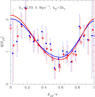
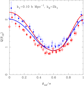
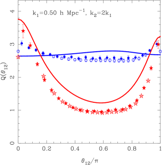
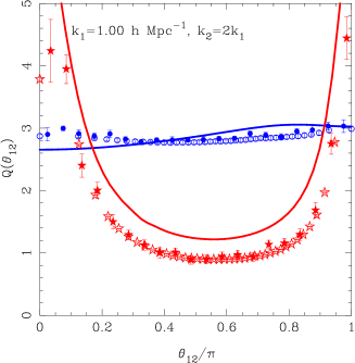
In this appendix we compare results from our recipe for estimating the reduced bispectrum, presented in Sec. VI.3, with those obtained from an independent prescription used by one of us over the years, e.g. Scoccimarro (2000), which uses full sampling of all -space triangles on the Fourier grid. The two methods are very similar, but some subtle differences exist, these can be summarized: for the “full sampling code”:
-
(1)
is estimated in linear bins of thickness a for and for the case (); whereas for our code estimates are made in bins of thickness ;
-
(2)
the configuration dependence of is estimated as a linear function of , whereas for our code it is estimated as a linear function of ;
-
(3)
all of the available independent -modes are used, whereas we sub- or over-sample modes from the available set depending on the number of available modes;
-
(4)
is constructed from estimates of and in a post-processing fashion, whereas we estimate on-the-fly for each triangle that is used in the estimate.
Fig. 7 shows the results of this comparison. The solid symbols denote our results, and the corresponding open symbols denote the results from the “full sampling code”. Overall we find very good agreement between both methods. On the largest scales that we have considered, , it appears that our method is a factor of 2-3 times more noisy than that of R. Scoccimarro, however we have a factor of 2 more bins in , which accounts for some of this discrepancy. On smaller scales the estimates are of comparable quality, with ours being slightly more noisy. The discrepancy on large scales owes to the fact that we have sub-sampled triangles from the possible set, this can be mitigated by oversampling from the number of available modes. On smaller scales the benefits of our approach are that we may obtain a high accuracy estimate without requiring all of the triangles and this also has the practical advantage of keeping the computational time tolerably low.
References
- Tegmark et al. (2004) M. Tegmark & The SDSS Collaboration, Astrophys. J. 606, 702 (2004).
- Cole et al. (2005) S. Cole & The 2dFGRS Collaboration, Mon. Not. R. Astron. Soc. 362, 505 (2005).
- Eisenstein et al. (2005) D. J. Eisenstein & The SDSS Collaboration, Astrophys. J. 633, 560 (2005).
- Tegmark et al. (2006) M. Tegmark & The SDSS Collaboration, Phys. Rev. D. , 74, 123507 (2006).
- Spergel et al. (2007) D. Spergel & The WMAP Collaboration, Astrophys. J. Supp., 170, 377 (2007).
- Bernardeau et al. (2002) F. Bernardeau, S. Colombi, E. Gaztañga, R. Scoccimarro, Physics Reports 367, 1 (2002).
- Sefusatti & Scoccimarro (2006) E. Sefusatti, R. Scoccimarro, Phys. Rev. D, D71, 063001, (2005).
- Fry & Gaztañaga (1993) J. Fry, E. Gaztañaga, Astrophys. J. 425, 1 (1993).
- Frieman & Gaztañaga (1994) J. A. Frieman, E. Gaztañaga, Astrophys. J. , 425, 392, (1994).
- Fry (1994) J. N. Fry, Phys. Rev. Lett. 73, 215 (1994).
- Sefusatti et al. (2006) E. Sefusatti, M. Crocce, S. Pueblas, R. Scoccimarro, Phys. Rev. D, D74, 023522, (2006).
- Fry & Scherrer (1994) J. N. Fry, R. J. Scherrer, Astrophys. J. , 429, 36 (1994).
- Gaztañaga & Fosalba (1998) E. Gaztañaga, P. Fosalba, Mon. Not. R. Astron. Soc. , 301, 524 (1998).
- Scoccimarro et al. (2004) R. Scoccimarro, E. Sefusatti, M. Zaldarriaga, Phys. Rev. D. , 69, 103513 (2004).
- Sefusatti & Komatsu (2007) E. Sefusatti, E. Komatsu, Phys. Rev. D. , 76, 083004 (2007).
- Bernardeau (2004) F. Bernardeau, astro-ph/0409224 (2004).
- Shirata et al. (2007) A. Shirata, Y. Suto, C. Hikage, T. Shiromizu, N. Yoshida, Phys. Rev. D. , 76, 044026 (2007).
- Jain & Zhang (2007) B. Jain, P. Zhang, arXiv:0709.2375 (2007).
- Scoccimarro (2008) R. Scoccimarro, in preparation (2008)
- Smith, Watts & Sheth (2006) R. E. Smith, P. I. R. Watts, R. K. Sheth, Mon. Not. R. Astron. Soc. 365, 214 (2006).
- Saunders et al. (2000) W. Saunders, & The PSCz Collaboration, Mon. Not. R. Astron. Soc. 317, 55, (2000).
- Colless et al. (2001) M. Colless & The 2dFGRS Collaboration, Mon. Not. R. Astron. Soc. 328, 1039, (2001).
- York et al. (2000) D. G. York & The SDSS Collaboration, Astron. J. , 120, 1579 (2000).
- Schneider et al. (2007) D. P. Schneider & The SDSS Collaboration, Astron. J. accepted, arXiv:0704.0806 (2007).
- Kayo et al. (2004) I. Kayo, Y. Suto, R. C. Nichol, J. Pan, I. Szapudi, A. J. Connolly, J. Gardner, B. Jain, G. Kulkarni, T. Matsubara, R. K. Sheth, A. S. Szalay, J. Brinkmann, PASJ, 56, 415, (2004).
- Jing & Böerner (2004) Y. P. Jing, G. Böerner, Astrophys. J. , 607, 140, (2004).
- Wang et al. (2004) Y. Wang, X. Yang, H. J. Mo, F. C. van den Bosch, Y-Q. Chu, Mon. Not. R. Astron. Soc. , 353, 287, (2004).
- Gaztañaga et al. (2005) E. Gaztanaga, P. Norberg, C. M. Baugh, D. J. Croton, Mon. Not. R. Astron. Soc. , 364, 620 (2005).
- Nichol et al. (2006) R. C. Nichol & The SDSS Collaboration, Mon. Not. R. Astron. Soc. , 368, 1507, (2006).
- Kulkarni et al. (2007) G. Kulkarni, R. Nichol, R. K. Sheth, H.-J. Seo, D. J. Eisenstein, A. Gray,Mon. Not. R. Astron. Soc. , 378, 1196 (2007).
- Scoccimarro et al. (2001) R. Scoccimarro, H. Feldman, J. Frieman, J. N. Fry, Astrophys. J. 546, 652 (2001).
- Feldman et al. (2001) H. Feldman, J. Frieman, J. N. Fry, R. Scoccimarro, Phys. Rev. Lett. 86, 1434 (2001).
- Verde et al. (2002) L. Verde, A. F. Heavens & The 2dfGRS Collaboration, Mon. Not. R. Astron. Soc. , 335, 432, (2002).
- Nishimichi et al. (2006) T. Nishimichi, I. Kayo, C. Hikage, K. Yahata, A. Taruya, Y.-P. Jing, R. K. Sheth, Y. Suto, Publ. Astron. Soc. Japan59, 93 (2007).
- Scoccimarro et al. (1999) R. Scoccimarro, H. M. P. Couchman, J. A. Frieman, Astrophys. J. , 517, 531, (1999)
- Gaztañaga & Scoccimarro (2005) E. Gaztañaga, R. Scoccimarro, Mon. Not. R. Astron. Soc. , 361, 824 (2005).
- Verde et al. (1998) L. Verde, A. F. Heavens, S. Matarrese, L. Moscardini, Mon. Not. R. Astron. Soc. , 300, 747(1998).
- Smith, Scoccimarro & Sheth (2007) R. E. Smith, R. Scoccimarro, R. K. Sheth, Phys. Rev. D. , 75.063512, (2007).
- Davis & Peebles (1983) M. Davis, P. J.E. Peebles, Astrophys. J. , 267, 465 (1983).
- Kaiser (1987) N. Kaiser, Mon. Not. R. Astron. Soc. , 227, 1, (1987).
- Hamilton (1998) A. J. S. Hamilton, in The Evolving Universe, Kluwer Academic, Dordrecht, 185 (1998)
- Scoccimarro (2004) R. Scoccimarro, Phys. Rev. D. , 70, 083007 (2004).
- Cooray & Sheth (2002) A. Cooray, R. K. Sheth, Physics Reports, 372, 1 (2002).
- Sheth et al. (2001) R. K. Sheth, A. Diaferio, L. Hui, R. Scoccimarro, Mon. Not. R. Astron. Soc. 326, 463 (2001).
- White (2001) M. White, Mon. Not. R. Astron. Soc. , 321 1, (2001).
- Seljak (2001) U. Seljak, Mon. Not. R. Astron. Soc. , 325 1359, (2001).
- Kang et al. (2002) X. Kang, Y. P. Jing, H. J. Mo, G. Böerner, Mon. Not. R. Astron. Soc. , 336 892, (2002).
- Smith et al. (2008) R. E. Smith, et al., in preparation, (2008)
- Benson et al. (2000) A. J. Benson, S. Cole, C. S. Frenk, C. M. Baugh, C. G. Lacey, Mon. Not. R. Astron. Soc. , 311, 793, (2000).
- Seljak (2000) U. Seljak, Mon. Not. R. Astron. Soc. , 318, 203 (2000).
- Peacock & Smith (2000) J. A. Peacock, R. E. Smith, Mon. Not. R. Astron. Soc. 318, 1144 (2000).
- Scoccimarro et al. (2001) R. Scoccimarro, R. K. Sheth, L. Hui, B. Jain, Astrophys. J. 546, 20 (2001).
- Berlind & Weinberg (2002) A. Berlind, D. Weinberg, Astrophys. J. 575, 587 (2002).
- Smith et al. (2003) R. E. Smith, J. A. Peacock, A. Jenkins, S. D. M. White, C. S. Frenk, F. R. Pearce, P.A. Thomas, G. Efstathiou H. M. P. Couchman, Mon. Not. R. Astron. Soc. 341, 1311 (2003).
- Crocce & Scoccimarro (2008) M. Crocce, R. Scoccimarro, Phys. Rev. D. , 77, 023533 (2008).
- Neyrinck & Szapudi (2007) M. C. Neyrinck, I. Szapudi, Mon. Not. R. Astron. Soc. , 384, 1221 (2008).
- Seljak & Zaldarriaga (1996) U. Seljak, M. Zaldarriaga, Astrophys. J. 469, 437 (1996).
- Tinker (2007) J. Tinker, Mon. Not. R. Astron. Soc. , 374, 477 (2007).
- Scherrer & Bertschinger (1991) R. Scherrer, E. Bertschinger, Astrophys. J. , 381, 349 (1991).
- Takada & Jain (2003) M. Takada, B. Jain, Mon. Not. R. Astron. Soc. , 340, 580, (2003).
- Press & Schechter (1974) W. Press, P. Schechter, Astrophys. J. , 187, 425, (1974)
- Bond et al. (1991) J. R. Bond, S. Cole, N. Kaiser, G. Efstathiou, Astrophys. J. , 379, 440, (1991).
- Sheth & Tormen (1999) R. K. Sheth, G. Tormen, Mon. Not. R. Astron. Soc. 308, 119 (1999).
- Sheth, Mo & Tormen (2001) R. K. Sheth, H.-J. Mo, B. Tormen, Mon. Not. R. Astron. Soc. , 323, 1, (2001).
- Jenkins et al. (2001) A. Jenkins, C. S. Frenk, S. D. M. White, J. Colberg, S. Cole, A. Evrard, H. Couchman N. Yoshida, Mon. Not. R. Astron. Soc. , 321, 372, (2001).
- Warren et al. (2006) M. S. Warren, K. Abazajian, D. E. Holz, L. Teodoro, Astrophys. J. , 646, 881 (2006).
- Reed et al. (2007) D. Reed, R. Bower, C. S. Frenk, A. Jenkins, T. Theuns, Mon. Not. R. Astron. Soc. , 374, 2 (2007).
- Moore et al. (1999) Moore B., Quinn T., Governato F., Stadel J., Lake G., Mon. Not. R. Astron. Soc. , 310, 1147 (1999).
- Klypin et al. (1999) Klypin A., Gottlöber S., Kravtsov A., Khokhlov A. M., Astrophys. J. , 516, 530 (1999).
- Jing & Suto (2002 – hereafter JS02) Jing Y. P., Suto Y., Astrophys. J. , 574, 538 (2002).
- Kuwabara, Taruya & Suto (2002) T. Kuwabara, A. Taruya, Y. Suto, Publ. Astron. Soc. Japan, 54, 503 (2002).
- Smith & Watts (2005) R. E. Smith, P. I. R. Watts, Mon. Not. R. Astron. Soc. 360, 203 (2005).
- Hivon et al. (1995) E. Hivon, F. R. Bouchet, S. Colombi, R. Juszkiewicz, Astron. Astrophys. , 298, 643 (1995).
- Mc Donald (2006) P. McDonald, Phys. Rev. D. , 74, 103512 (2006).
- Scoccimarro et al. (1998) R. Scoccimarro, S. Colombi, J. N. Fry, J. A. Frieman, E. Hivon, A. Melott, Astrophys. J. , 517, 531, (1999)
- Peebles (1980) P. J. E. Peebles, “The Large-scale Structure of the Universe” (Princeton University Press, Princeton, 1980.)
- Scoccimarro (1998) R. Scoccimarro, Mon. Not. R. Astron. Soc. , 299, 1097 (1998).
- Crocce et al. (2006) M. Crocce, S. Pueblas, R. Scoccimarro, Mon. Not. R. Astron. Soc. , 373, 369 (2006).
- Springel (2005) V. Springel, Mon. Not. R. Astron. Soc. , 364, 1105 (2005).
- Hockney & Eastwood (1981) R. W. Hockney, J. W. Eastwood,“Computer Simulations Using Particles”, McGraw-Hill, New York (1981).
- (81) M. Frigo, S. G. Johnson, http://www.fftw.org/ (2007).
- Jing (2005) Y. P. Jing, Astrophys. J. , 620, 559 (2005).
- Eisenstein & Hu (1998) D. J. Eisenstein, W. Hu, Astrophys. J. , 496, 605 (1998).
- Meiskin, White & Peacock (1999) A. Meiksin, M. White, J. A. Peacock, Mon. Not. R. Astron. Soc. , 304, 851 (1999).
- Smith, Scoccimarro & Sheth (2008) R. E. Smith, R. Scoccimarro, R. K. Sheth, Phys. Rev. D. , 77, 043525 (2008).
- Neto et al. (2007) A. Neto, et al., Mon. Not. R. Astron. Soc. , 381, 1450 (2007).
- Hu & Cooray (2001) A. Cooray, W. Hu, Astrophys. J. , 554, 56C (2001).
- Scoccimarro (2000) R. Scoccimarro, Astrophys. J. , 544, 597 (2000).
- Navarro, Frenk & White (1997) J. Navarro, C. S. Frenk, S. D. M. White, Astrophys. J. 490, 493 (1997). (NFW)
- Bryan & Norman (1998) G. Bryan, M. Norman, Astrophys. J. , 495, 80, (1998).
- Bullock et al. (2001) J. Bullock, T. Kolatt, Y. Sigad, R. Somerville, A. Kravtsov, A. Klypin, J. Primack, A. Dekel, Mon. Not. R. Astron. Soc. , 321, 559, (2001).
- Lahav et al. (1991) O. Lahav, P. Lilje, J. Primack, M. Rees, Mon. Not. R. Astron. Soc. , 251, 128
- Sheth & Jain (2003) R. K. Sheth, B. Jain, Mon. Not. R. Astron. Soc. , 345, 592 (2003).
- Sheth (1996) R. K. Sheth, Mon. Not. R. Astron. Soc. , 279, 1310, (1996).
- Binney & Tremaine (1988) J. Binney, S. Tremaine, Galactic Dynamics, Princeton University Press, Princeton, USA, (1988).
- Mathews & Walker (1970) Mathews J, Walker R. L., 1970. “Mathematical methods of physics”, W. A. Benjamin Publishers Inc., New York