Statistical Analysis of Galaxy Surveys-I. Robust error estimation for 2-point clustering statistics

Abstract

We present a test of different error estimators for 2-point clustering statistics, appropriate for present and future large galaxy redshift surveys. Using an ensemble of very large dark matter $\Lambda$CDM N-body simulations, we compare internal error estimators (jackknife and bootstrap) to external ones (Monte-Carlo realizations). For 3-dimensional clustering statistics, we find that none of the internal error methods investigated are able to reproduce neither accurately nor robustly the errors of external estimators on 1 to $25{\,h^{-1}\,{\rm Mpc}}$ scales. The standard bootstrap overestimates the variance of $\xi(s)$ by $\sim 40$% on all scales probed, but recovers, in a robust fashion, the principal eigenvectors of the underlying covariance matrix. The jackknife returns the correct variance on large scales, but significantly overestimates it on smaller scales. This scale dependence in the jackknife affects the recovered eigenvectors, which tend to disagree on small scales with the external estimates. Our results have important implications for the use of galaxy clustering in placing constraints on cosmological parameters. For example, in a 2-parameter fit to the projected correlation function, we find that the standard bootstrap systematically overestimates the 95 % confidence interval, while the jackknife method remains biased, but to a lesser extent. The scatter we find between realizations, for Gaussian statistics, implies that a 2-$\sigma$ confidence interval, as inferred from an internal estimator, could correspond in practice to anything from 1-$\sigma$ to 3-$\sigma$. Finally, by an oversampling of sub-volumes, it is possible to obtain bootstrap variances and confidence intervals that agree with external error estimates, but it is not clear if this prescription will work for a general case.

1 Introduction

The large-scale structure (LSS) of the Universe, as traced by galaxies and clusters, encodes important information about the basic cosmological parameters and also the physical process which underpin the formation of cosmic structures. LSS measurements are now routinely used in conjunction with measurements of the cosmic microwave background (CMB) to constrain cosmological parameters (e.g. Cole et al. 2005; Sanchez et al. 2006; Tegmark et al. 2006; Percival et al. 2007). However, the estimation of errors in CMB measurements is, by comparison with LSS work, quite sophisticated and rigorous.

To constrain the cosmological world model from the galaxy distribution, large volumes and galaxy numbers are needed. The current generation of local galaxy surveys, such as the 2dFGRS (Colless et al. 2001) and SDSS (York et al. 2000) satisfy both of these requirements and can be divided into large sub-samples to study clustering trends with galaxy properties (e.g. Norberg et al. 2001, 2002; Zehavi et al.  2002, 2004, 2005; Madgwick et al.2003; Croton et al. 2004, 2007; Gaztañaga et al. 2005; Li et al. 2006, 2007). In anticipation of even bigger surveys at intermediate and high redshifts (e.g. GAMA, VVDS-CFHTLS, Euclid), it is timely to revisit the techniques used to estimate errors on clustering statistics from galaxy redshift surveys. In particular, we explore ways to robustly quantify reliable errors estimates on two-point clustering statistics in 3-dimensional space. This has important consequences for the determination of the cosmological parameters, both in terms of setting values and in the number of free parameters needed to describe the data, and in uncovering trends which can be used to constrain galaxy formation models.

In a perfect world, the optimal way to estimate the error on a clustering measurement would be to generate a large sample of independent mock galaxy catalogues that look the same as the data (at least in so far as the observed data may be affected by sampling fluctuations, e.g. Efstathiou & Moody 2001). The challenge here is to ensure that the mocks are a faithful reproduction of the observations. This is a more demanding requirement than one might at first think. In order to estimate accurate errors on the two-point statistics, it is necessary that the mocks also reproduce the higher order clustering displayed by the data, since the errors on 2-point statistics implicitly depend on these higher order moments. This approach will inevitably involve N-body simulations, in order to accurately model the underlying dark matter, and so becomes computationally expensive. Various techniques have been adopted in the literature to populate such simulations with galaxies (for a survey see Baugh 2008). The number of simulations required is large, running into several tens to get reasonable estimates of the variance and hundreds or even thousands to get accurate covariance matrices.

An alternative empirical method is to use the observed data itself to make an estimate of the error on the measurement. Such “internal” error estimates use a prescription to perturb the data set in some way in order to make copies. These copies allow the statistical distribution which underlies the data to be probed without having to assume anything about its form. In this paper we investigate the performance of two common approaches, the jackknife and bootstrap internal error estimates; both will be compared to the errors calculated from a large suite of simulated mock data sets.

The jackknife method was developed as a quite generic statistical tool in the 1950s (Quenouille 1956; Tukey 1958). The bootstrap method (e.g. Efron 1979) is a modification or extension of the jackknife made possible by the availability of fast computers in the 1970s. These internal estimators first divide the data set into subsamples, which consist either of individual objects or groups of objects, which are then resampled in a particular way (see Section 2 for a full description of the procedure). The first applications of either technique to astronomical observations date from the early 1980s with the analysis of the velocities of galaxies in clusters (Lucey 1979; Bothun et al. 1983). The bootstrap method was first applied to galaxy clustering by Barrow, Bhavsar & Sonoda (1984; see also Ling, Frenk & Barrow 1986).

In these early works sub-samples were simply taken using the individual objects themselves. However, as pointed out by Fisher et al. (1994), this can lead to unreliable errors. From a Monte-Carlo analysis using a series of N-body simulations, Fisher et al. showed that when sampling individual galaxies the bootstrap method underestimates the error on the density estimate in voids and, likewise, overestimates it in clusters. Mo, Jing & Börner (1992) present an analytic estimate for the errors on 2-point statistics and show that the bootstrap errors obtained by resampling using individual galaxies give incorrect errors compared with the ensemble average under certain conditions. These valid objections can be avoided by resampling the data set divided into sub-volumes instead of individual galaxies. Hence, in this paper, we generate copies of data sets by selecting sub-volumes of the data set.

Resampling of patches or regions of surveys has already been applied to error estimation in LSS analyses. The jackknife technique has been extensively used in projection, including the angular clustering of galaxies (Scranton et al. 2002), in the analysis of CMB maps (e.g. Gaztañaga et al. 2003) and, perhaps most heavily, in efforts to detect the Integrated Sachs-Wolfe effect by cross-correlating sky maps of galaxy or cluster positions with temperature fluctuations in the cosmic microwave background (Fosalba, Gaztañaga & Castander 2003; Fosalba & Gaztañaga 2004; Cabré et al. 2007). In projection, the jackknife variance agrees well with Monte-Carlo estimates from mock catalogues (e.g. Cabré et al. 2007). This is perhaps an easier case than the three dimensional surveys dealt with in this paper, since the distributions of galaxy fluctuations will tend to look more Gaussian in projection (although distinct non-Gaussian behaviour is clearly evident in the projected galaxy fluctuations, e.g. Gaztañaga 1994).

The jackknife method has also been applied by many authors to the estimation of errors on galaxy clustering in three dimensions using volume resampling. Zehavi et al. (2002) carried out a simple test of the accuracy of the jackknife estimate of the variance and found that the jackknife produced an essentially unbiased estimate, but with a scatter that could approach 50%. Here we carry out a more exhaustive comparison of internal error estimators with the “external” Monte-Carlo simulation methods.

The paper is arranged in the following way. Section 2 defines the three error estimators we use throughout, while Section  3 introduces the simulations which will be used to generate fake data sets for our numerical experiments, along with the clustering statistics and the principal component decomposition, needed for the error estimator comparison. Section 4 presents the raw results from three different error techniques and remains rather technical. We consider in Section 5 a simple test case scenario, where the implications of using different error estimators for a “straightforward” two parameter fit to the projected correlation function are inferred. We summarize our findings in Section 6.

2 Review of error estimation methods

There are numerous ways to estimate the error on a clustering measurement. In this section, we give an outline of four of the most popular non-parametric methods in use in the literature, three of which we compare in this paper. We do not consider in this paper analytic error estimates (like Poisson), nor parametric error estimates, like those derived from Gaussian or Log-Normal density fields. The latter methods are commonly used for estimating errors in the linear clustering regime (see e.g. Percival et al. 2001 and Cole et al. 2005 for applications to power spectrum estimates). Below, we describe three “internal” methods which use the data itself to derive an estimate of the error on a measurement, the sub-sample, jackknife and bootstrap techniques (sections 2.2, 2.3 and 2.4). Then we describe in section 2.5 the commonly used “external” method of creating Monte-Carlo realizations or reproductions of the data. We close by giving an overview of the advantages and disadvantages of each method in Section 2.6.

Each of the techniques involves performing measurements on copies of the data in order to sample the underlying probability distribution of the quantity we are trying to measure. The internal estimates make copies or resamplings from the observed data whereas the external method generates fake data sets, without manipulating the observed data. Three assumptions are implicit in the internal or “data inferred” approaches: 1) the data gives an accurate representation of the underlying probability distribution of measurements; 2) the sub-samples into which the data is split are sufficient in number to allow accurate enough estimates of the errors and 3) the sub-sample volumes are large enough to be representative. Condition 1 would be violated if a second independent measurement from an equivalent data set gave a significantly different estimate of the measurement. In such a case, this would mean that the original data set is subject to sampling fluctuations (sometimes called cosmic variance) which affect the clustering measurements. Conditions 2 and 3 are related. The number of sub-samples that should be used in the internal estimators depends on the questions to be answered and the (unknown) form of the underlying probability distribution: for example, to obtain an estimate of the variance accurate to 10% would require 50 resamplings of the data set for a Gaussian distribution. At the same time, we need to be careful not to make the sub-samples so small so that they become strongly correlated. Norberg & Porciani (in prep.) investigate this problem using the two-pair correlation function. Later we address the question of whether or not one can put qualitative constraints, and maybe even quantitative constraints (using a large suite of simulations), on the representativeness of a given size of sub-sample.

2.1 Internal estimates: preliminaries

The first applications of non-parametric internal techniques to the estimation of the error on the two-point correlation function considered the removal of individual objects from the data set (Barrow, Bhavsar & Sonoda 1984; Ling, Frenk & Barrow 1986). This is computationally infeasible for modern galaxy catalogues, and it has been shown at galaxy number densities currently considered that this type of error estimate strongly underestimates the true clustering uncertainty (e.g. Mo, Jing & Börner 1992; Fisher et al. 1994). Furthermore, we want to reduce the correlation between the sub-samples into which the data set is split. For this reason, we divide the samples by volume and split our data sets into $N_{sub}$ cubes of equal volumes. The internal methods then reconstruct copies of the original data sets, choosing or weighting the $N_{sub}$ sub-volumes in different ways. For each copy or resampling of the data, we make an estimate of the correlation function, which we denote by $x^{k}_{i}$ in this section. Here the subscript $i$ refers to the bin of spatial separation and the superscript $k$ refers to the resampling of the data for which the correlation function is measured. Note that we use the terms “a resampling” and “copy” of the data set interchangeably; here, a resampling refers to a “full” copy of a data set, rather than to the act of selecting an individual sub-volume.

2.2 Internal estimate 1: The sub-sample method

The covariance matrix of $N$ independent realizations is, by definition, given by

$$C(x_{i},x_{j}) = \frac{1}{N}\sum_{k=1}^{N}(x_{i}^{k}-\bar{x_{i}})(x_{j}^{k}-\bar{x_{j}})~{},$$ (1)

where it is assumed that the mean expectation value, $\bar{x_{i}}$, is not estimated from the $\{x_{i}^{k}\}_{k=1}^{N}$ samples, but from an independent realization of the data.

Hence, the simplest error method, commonly referred to as the sub-sample method, consists of splitting the data set into $N_{sub}$ independent samples and estimating the covariance matrix using Eq. 1, where the clustering statistic is estimated for each one of the sub-samples separately. For $N_{sub}$ independent sub-samples, this returns the correct covariance for a sample of volume 1/$N_{sub}$ of the original volume, implying that the covariance of the full dataset is actually $N_{sub}$ times smaller (as the variance scales directly with the volume considered). This method has been used in several studies, in particular where the survey volumes considered are large (e.g. Maddox et al. 1990, Hamilton 1993a and Fisher et al. 1994 for the APM, the IRAS 2Jy and the IRAS 1.2Jy galaxy surveys respectively).

However, one basic assumption made in this approach is never really satisfied for galaxy clustering studies in the Universe: the sub-samples are never fully independent of each other, irrespective of the clustering scales considered. This is due to the presence of long-range modes in the density fluctuations, making all sub-samples to some extent correlated with each other. This can be related to the fact that the correlation function has a small but non-zero value on large scales. Therefore there is a need to consider alternative internal estimators, accounting hopefully for these limitations. Hereafter we will not consider the sub-sample method, even though it has been extensively used in the past.

2.3 Internal estimate 2: The jackknife method

We consider the “delete one jackknife” method (Shao 1986). A copy of the data is defined by systematically omitting, in turn, each of the $N_{sub}$ sub-volumes into which the data set has been split. The resampling of the data set consists of the ${N_{sub}}-1$ remaining sub-volumes, with volume $({N_{sub}}-1)/{N_{sub}}$ times the volume of the original data set. The clustering measurement is repeated on the copy or resampling of the original data set. By construction, there are only $N=$$N_{sub}$ different copies of the data set that are created in this way. The covariance matrix for $N$ jackknife resamplings is then estimated using

$$C_{\rm jk}(x_{i},x_{j}) = \frac{(N-1)}{N}\sum_{k=1}^{N}(x_{i}^{k}-\bar{x_{i}})(x_{j}^{k}-\bar{x_{j}})~{},$$ (2)

where $x_{i}$ is the $i^{\rm th}$ measure of the statistic of interest (out of $N$ total measures), and it is assumed that the mean expectation value is given by

$$\bar{x_{i}} = \sum_{k=1}^{N}x_{i}^{k}/N\,.$$ (3)

Note the factor of $N-1$ which appears in Eq. 2 (Tukey 1958; Miller 1974). Qualitatively, this factor takes into account the lack of independence between the $N$ copies or resamplings of the data; recall that from one copy to the next, only two sub-volumes are different (or equivalently $N-2$ sub-volumes are the same). Hereafter, we will refer to a jackknife estimate from $N_{sub}$ sub-samples as Jack-$N_{sub}$.

2.4 Internal estimate 3: The bootstrap method

A standard bootstrap resampling of the data set is made by selecting $N_{r}$ sub-volumes at random, with replacement, from the original set (Efron 1979). Effectively, a new weight is generated for each sub-volume. In the original data set, all sub-volumes have equal weight. In a resampled data set, the weight is simply the number of times the sub-volume has been selected e.g. $w_{\rm i}=0,1,2\ldots$. The clustering measurement is repeated for each resampled data set. For a given $N_{r}$, the mean fractional effective volume of the resampled data sets tends to a fixed fraction of the original sample volume. For $N_{r}$=$N_{sub}$, the mean effective volume is less than the volume of each of the jackknife resamples. We further develop this discussion in §4.2 and §5.5.

Unlike for jackknife error estimates, in principle there is no limit on the number $N$ of resamplings or copies of the data for bootstrap error estimates. In practice, the variance on a measurement converges relatively slowly with increasing numbers of trials (Efron & Tibshirani 1993). Furthermore, for our application, resamplings are cheap to generate but expensive to analyse. For a data set divided into $N_{sub}$ sub-volumes and from which one draws $N_{r}$ sub-volumes at random with replacement, there are $({N_{sub}}+{N_{r}}-1)!/({N_{sub}}-1)!{N_{r}}!$ different possible bootstrap resamplings, which even in the modest example of $N_{r}$=$N_{sub}$=10 corresponds to 92 378 different bootstrap resamplings. Here we restrict ourselves to of the order of one hundred resamplings (i.e. $N\sim 100$). Until now, most, if not all, bootstrap clustering estimates have used resamplings consisting of $N_{r}$=$N_{sub}$ sub-volumes. In this paper we test this assumption by considering up to 4 $N_{sub}$ sub-volumes to construct each resampling of the data set (Section 5.5).

The covariance matrix for $N$ bootstrap resamplings of the data is given by

$$C_{\rm boot}(x_{i},x_{j}) = \frac{1}{N-1}\sum_{k=1}^{N}(x_{i}^{k}-\bar{x_{i}})(x_{j}^{k}-\bar{x_{j}}),$$ (4)

where it is assumed that the mean expectation value is given by Eq. 3. Note that there is no $N-1$ factor in the numerator of this expression, as was the case for the jackknife. Qualitatively the data set copies are thought of as being “more” independent in the case of bootstrap resampling than for jackknife resampling, something we address in detail in Sections 4 and 5. In what follows we will refer to the mean bootstrap estimate from $N_{sub}$ sub-samples as Boot-$N_{sub}$.

2.5 External estimate: Monte Carlo realizations

The Monte Carlo method consists of creating $N$ statistically equivalent versions of the data set being analysed, on each of which the full analysis is repeated. Technically, bootstrap resampling is also a Monte-Carlo method. However, the distinction here is that what we have termed the Monte Carlo approach makes no explicit reference to the observed data set to generate the synthetic data sets. We are not resampling the data in any way. Instead, we assume that we know the underlying statistical or physical processes which shaped the observed data set and feed these into a computer simulation. Here we have run N-body simulations which model the clustering evolution of the dark matter in the universe (see Section 3.1). The Monte Carlo element in this case refers to the initial conditions, which are drawn from a distribution of density fluctuations consistent with cosmological constraints (see e.g. Sanchez et al. 2006). The level of realism of the computer simulation determines the cost of this method. For a clustering analysis of an observed galaxy catalogue, the demands on the Monte Carlo approach are even greater as the N-body simulations need to be populated with galaxies, according to some prescription, with the goal of statistically reproducing the galaxy sample as faithfully as possible (see e.g. Baugh 2008 for a review of the techniques used to build synthetic galaxy catalogues).

We hereafter refer to the Monte Carlo catalogues generated in the external error estimation as “mocks”, and their associated errors as mock errors. In the current work using N-body simulations, we use Eq. 4 as the definition of the Monte Carlo covariance matrix, since we define our “reference sample” as the mean measurement of the correlation function extracted from the ensemble of simulations.

2.6 Pros and cons of each method

Each of the error estimation techniques described above has its advantages and disadvantages. By definition, errors calculated directly from the data take into account any hidden or unforeseen systematics and biases that might otherwise be missed. This is particularly important for clustering statistics, where the errors on the 2-point correlation function also depend on the higher order clustering of the data. These properties of the galaxy distribution are usually not otherwise appropriately accounted for in an error analysis. Other properties of the data, such as the galaxy mix and survey selection, are also naturally satisfied in an internal approach. In the case of external error estimation using mocks, only the statistics that have been deliberately included in the Monte Carlo realization are guaranteed to be taken into account in the error analysis. If a biasing scheme has been constrained to reproduce the two-point function of galaxy clustering, there is no guarantee that the higher order moments of the distribution will also match those of the observed data set.

On the other hand, internal error estimates are often severely limited by the size of the data set itself. This can be particularly problematic for clustering statistics, as studied here. Obviously, sampling or cosmic variance on scales larger than sample volume cannot be addressed by internal estimates, but can be included in external estimates made using mocks.

3 The numerical experiments

Our aim in this paper is to repeat the early comparisons of internal and external error estimates in the context of current and forthcoming galaxy redshift surveys. We draw data sets from numerical simulations which are described in Section 3.1. The clustering analysis of these data sets is described in Section 3.2. Finally, in Section 3.3, we give an outline of the principal component decomposition of the covariance matrix of clustering measurements, which is an invaluable diagnostic in error estimation.

3.1 Creating test data sets

Our analysis uses the $z=0.5$ output from the L-BASICC ensemble of N-body simulations carried out by Angulo et al. (2008). The set comprises 50 moderate resolution runs, each representing the dark matter using $448^{3}=89~{}915~{}392$ particles of mass $1.85\times 10^{12}\,h^{-1}\,M_{\odot}$ in a box of side $1340h^{-1}$Mpc. Each L-BASICC run was evolved from a different realization of a Gaussian density field set up at $z=63$. The adopted cosmological parameters are broadly consistent with recent data from the cosmic microwave background and the power spectrum of galaxy clustering (e.g. Sanchez et al. 2006): $\Omega_{\rm M}=0.25$, $\Omega_{\Lambda}=0.75$, $\sigma_{8}=0.9$, $n=1$, and $w=-1$. Throughout we assume a value for the Hubble parameter of $h=H_{0}/(100\,{\rm km\,s}^{-1}{\rm Mpc}^{-1})=0.73$.

Table 1: A summary of the numerical experiments conducted in this paper. Col. 1 lists the error estimation technique applied; col. 2 gives the number of sub-samples into which each data set is split up; col. 3 indicates whether the analysis was performed in real (r) or redshift (z) space; col. 4 gives the number of different data sets used; col. 5 shows the number of resamplings and clustering measurements performed for each data set, $N$; col. 6 lists, for the case of bootstrap errors only, the relative number of sub-volumes selected at random with replacement from the original list w.r.t. $N_{sub}$; col. 7 shows the sampling fraction w.r.t. our nominal mean density which is set to match that of a L_⋆ galaxy sample. The first group of experiments yielded our main results and used in the majority of the plots; the other experiments are variants to test different components of the analysis and referred to in the text.

Error	$N_{sub}$	r/z	$N_{dataset}$	$N$	$N_{r}$/$N_{sub}$	f
Mock	1	z [r]	100 [100]	1		1
Boot	8	z [r]	100 [50]	99	1	1
Boot	27	z [r]	100 [50]	99	1	1
Jack	8	z [r]	100 [50]	8		1
Jack	27	z [r]	100 [50]	27		1
Jack	64	z	100	64		1
Mock	1	r	100 [100]	1		0.1 [0.25]
Boot	8	r	50 [50]	99	1	0.1 [0.25]
Boot	27	r	50 [50]	99	1	0.1 [0.25]
Boot	64	r	50 [50]	99	1	0.1 [0.25]
Boot	125	r	50 [50]	199	1	0.1 [0.25]
Boot	8	r	25 [25]	99	2, 3	0.1 [0.25]
Boot	27	r	25 [100]	99	2, 3	0.1 [0.25]
Boot	64	r	25 [100]	99	2, 3	0.1 [0.25]
Boot	125	r	25 [100]	199	2, 3	0.1 [0.25]
Jack	8	r	100 [50]	8		0.1 [0.25]
Jack	27	r	100 [100]	27		0.1 [0.25]
Jack	64	r	100 [100]	64		0.1 [0.25]
Jack	125	r	100 [100]	125		0.1 [0.25]
Boot	8	r	6 [6]	99	4	0.1 [0.25]
Boot	27	r	6 [6]	99	4	0.1 [0.25]
Boot	64	r	6 [6]	99	4	0.1 [0.25]
Boot	125	r	6 [6]	199	4	0.1 [0.25]

The combination of a large number of independent realizations and the huge simulation volume make the L-BASICC ensemble ideal for our purposes. Angulo et al. (2008) showed that nonlinear and dynamical effects are still important for the evolution of matter fluctuations even on scales in excess of $100h^{-1}$Mpc and that these scales contribute to the growth of smaller scale perturbations. A smaller simulation volume would not be able to model the growth of fluctuations accurately because these long wavelength modes would be missed. The large volume also means that it is still possible to extract more than one region from each simulation which can be considered as being effectively independent from the others due to their large spatial separation. Equally important it is also possible to mimic with such a large simulation volume the real situation of a survey like the 2dFGRS, for which there are two distinct survey regions in two nearly opposite directions on the sky.

From each of the 50 simulation cubes we extract two cubical sub-volumes of $380~{}{\,h^{-1}\,{\rm Mpc}}$ on a side which are separated by at least $\sim 500~{}{\,h^{-1}\,{\rm Mpc}}$ from one other. We could have extracted more than 40 volumes of this size from each simulation cube without choosing the same volume twice. However, we chose to follow this more conservative approach as we want to be able to treat the two sub-volumes as being effectively independent of one another. Although they come from the same simulation volume, the fluctuations on scales greater than $500~{}{\,h^{-1}\,{\rm Mpc}}$ are relatively weak. Hence, the total number of available data sets constructed in this way comes to 100, each of which is fully independent of 98 of the others and essentially independent of the remaining 99^th data set. The size of each data set is chosen to match the volume of a typical L_⋆ volume-limited sample extracted from the main SDSS galaxy redshift survey (e.g. Zehavi et al. 2004, 2005). Note that this volume is about 10 times larger than the equivalent volume-limited samples of L_⋆ galaxies used in the final 2dFGRS clustering analyses (Norberg et al. in prep.). Finally, we have randomly diluted the number of dark matter particles in each data set in order to match the number density of a L_⋆ galaxy sample of $3.7\times 10^{-3}~{}{\,h^{-3}\,{\rm Mpc^{3}}}$, which mimics the discreteness or shot noise level in typical observational data sets.

Note that on this occasion, we do not attempt to model a particular galaxy sample in detail, as our aim here is to provide a generic analysis that is as widely applicable and reproducible as possible, within a framework which is likely to remain the same in the foreseeable future. Moreover, if one attempted to model a galaxy sample rather than the dark matter, this would open up the issue of how well can the model reproduce the higher order clustering of the galaxies. This is a problem to be addressed by those building mock galaxy catalogues for particular surveys and is beyond the scope of the current paper. By focusing on dark matter clustering only, our analysis remains well defined and fully accurate within our chosen cosmological model.

A summary of the samples and error calculations carried out is given in Table 1. Each data set drawn from a simulation can be divided into sub-volumes in order that it be resampled according to the jackknife or bootstrap algorithm. Thus, we have up to 100 independent experiments for which we can compare internal estimates of the error on the correlation function, and consider for the first time in detail the whole error distribution of internal error estimates. The external “mock” estimate of the error is obtained using all 100 data sets. In all, we have performed about 250 thousand correlation function estimates, representing about one million CPU hours of calculations.

3.2 Estimating the two-point correlation function

Throughout this paper we consider only standard two-point clustering statistics and we delay to a future paper the study of more recent two-point clustering statistics, like the $\omega$-statistic of Padmanabhan, White & Eisenstein (2007). We measure the two point correlation function, $\xi_{\rm X}(r_{\rm p},\pi)$, as a function of pair separation perpendicular to ($r_{\rm p}$) and parallel to ($\pi$) the line of sight of a fiducial observer, in real (X=$r$) and in redshift space (X=$s$). In order to remain as comparable as possible with the analysis of observational data, we do not use the common distant observer approximation, but instead perform a realistic angular treatment with a location chosen for the observer within the simulation box, i.e.:

$${\bf r_{los}} = ({\bf\widehat{r_{1}}}+{\bf\widehat{r_{2}}})/2$$

$$r_{p} = {\bf r_{1}}\cdot{\bf\widehat{r_{los}}}+{\bf r_{2}}\cdot{\bf\widehat{r_{los}}}$$

$$\pi = \sqrt{({\bf r_{1}}-{\bf r_{2}})^{2}-(r_{p})^{2}}~{},$$ (5)

where ${\bf r_{1}}$ and ${\bf r_{2}}$ are the position vectors of the two objects in the pair and a hat indicates that the vector is appropriately normalized; ${\bf r_{los}}$ is the mean distance to the pair of objects along the line of sight from the observer. Redshift space distortions are modelled in the same way, i.e.:

$$z_{\rm tot} = z_{\rm hub}+{\bf v}\cdot{\bf\widehat{r}}/c\,,$$ (6)

where $z_{\rm hub}$ is the galaxy’s redshift without peculiar motions, ${\bf v}$ is its peculiar velocity in addition to the Hubble flow and $c$ is the speed of light.

We calculate the two dimensional correlation function $\xi_{\rm X}(r_{\rm p},\pi)$ for each data set using standard estimators, e.g. Hamilton (1993) and Landy & Szalay (1993). In order to obtain a robust estimate of the mean density, these estimators require that a large number of points be randomly distributed within the boundaries of the data set, according to the angular and radial selection functions which define the data. The number of randomly distributed points is typically larger than the number of data points by a factor of $f\simeq 100$, and we use the technique outlined in Landy & Szalay (1993) to speed up the calculation of the random-random pair counts. In practice, to avoid fluctuations in the mean density at small pair separations, we typically use 4 times as many random points as data points and repeat the estimate of the pair counts about 25 times. We use a unique set of randoms for each calculation, so that our statistics are not influenced by any features in the randoms, which when an experiment is repeated numerous times could actually show up in a systematic fashion. Finally to compute the $\xi_{\rm s}(r_{\rm p},\pi)$ estimate, we limit the counts to pairs separated by less than 10 degrees for two reasons: 1) results effectively estimated in redshift space can be properly interpreted using the redshift space distortion model of Kaiser (1987), developed in the distant observer approximation; 2) the projected correlation function, defined below, can be considered as a real space quantity. These issues are discussed in greater detail in e.g. Matsubara (2000) and Szapudi (2004), but also applied in some clustering studies, like Hawkins et al. (2003) and Cabré & Gaztañaga (2008). Using logarithmic binning in both the $r_{\rm p}$ and $\pi$-directions, we estimate the projected correlation function, w_p(r_p)/r_p  (sometimes also written as $\Xi(\sigma)/\sigma$ and with $\sigma=r_{\rm p}$), by integrating $\xi_{\rm X}(r_{\rm p},\pi)$ in the $\pi$ direction (see Eq. 7 below). The only real motivation for this exercise is that the projected correlation function is, in theory, free from distortions arising from gravitationally induced peculiar motions. This point is discussed further in Section 4.1.

We also estimate the spherically averaged correlation functions, $\xi_{r}(s)$ and $\xi_{s}(s)$ in “$r$” real and “$s$” redshift space respectively, by averaging over shells in pair separation given by $s=\sqrt{r^{2}_{p}+\pi^{2}}$. As for the projected correlation function we use logarithmic binning and accumulate pair counts directly, i.e. not by integrating over the 2-d correlation function estimate.

Given $\xi_{\rm X}(r_{\rm p},\pi)$, the different clustering statistics are related by

$$w_{\rm p}(r_{\rm p})/r_{\rm p} = \frac{2}{r_{\rm p}}\int_{0}^{\pi_{\rm max}}\xi_{\rm X}(r_{\rm p},\pi)\,d\pi~{}.$$ (7)

$$\xi_{\rm X}(s) = <\xi_{\rm X}(r_{\rm p},\pi)>|_{s=\sqrt{r^{2}_{\rm p}+\pi^{2}}}\,,$$ (8)

with X=$r$ or $s$, real and redshift space respectively. Here, the integral for $w_{\rm p}(r_{\rm p})/r_{\rm p}$ is carried out to a maximum value of the separation along the line of sight of $\pi_{\rm max}$. Theoretically w_p(r_p) is only a true real space quantity when $\pi_{max}=\infty$. In Section 4.1 we discuss the systematic implications of a finite choice for $\pi_{\rm max}$.

3.3 Principal component decomposition

The covariance matrix of correlation function measurements, is not, in itself, of much interest. However, the inverse of the covariance matrix plays a pivotal role, appearing, for example, in all simple $\chi^{2}$ estimates. As matrix inversions are highly non-linear by nature, the impact of noise in the estimate of the covariance matrix is hard to judge, unless extensive tests are carried out. A number of procedures exist to help with the matrix inversion and analysis.

First, we prewhiten the covariance matrix, which means that all diagonal terms are rescaled to unity and all non-diagonal terms are rescaled to fall between -1 and 1,

$${\bf C} = {\bf\sigma}\,{\bf C_{N}}\,{\bf\sigma}~{},$$ (9)

where ${\bf C_{N}}$ is the normalized covariance matrix, and $\sigma_{i,j}=C_{i,i}\delta_{i,j}$, hereafter also referred to as $\sigma_{i}$.

Second, we decompose the $N_{u}\times N_{u}$ normalized covariance matrix into its principal components, solving the eigen-equations:

$${\bf C_{N}}\,{\bf E_{i}} = \lambda_{i}\,{\bf E_{i}}\quad i=1,...,N_{u}~{},$$ (10)

where $\lambda_{i}$ and ${\bf E_{i}}$ are the normalized eigenvalues and eigenvectors of the normalized covariance matrix. We have deliberately defined $N_{u}$ as the dimension of the covariance matrix actually used in the analysis, and not assumed it to be necessarily equal to the total number of data points for the given statistic (e.g. the number of bins of pair separation in the correlation function). Even though the parts of the covariance matrix that are used do not depend on those that are not used, principal component decomposition and matrix inversion strongly rely on the full matrix set up. For that reason, it is essential to pre-define the parts of the covariance matrix to be considered, a fact that is most often neglected.

There are many useful properties of principal component decomposition worth listing here (see for example Kendall 1975; Press et al. 1992):

• The $\left\{{\bf E_{i}}\right\}_{i=1}^{N}$ form a complete orthogonal basis, from which the whole covariance matrix can be reconstructed.

• A principal component decomposition minimises the error for the number of components used.

• A ranking of the eigenvectors in order of decreasing eigenvalue highlights the principal trends of the covariance matrix.

• For a given covariance matrix there is a unique set of principal components. Comparing covariance matrices is equivalent to the comparison of principal components.

With respect to this last point, it is essential to understand noise in the statistic and its non-trivial effect on estimating the principal components of the covariance matrix. Clearly, in the absence of noise, two covariance matrices are identical if, and only if, their principal components are identical. In real systems that contain noise this is no longer true.

For this paper the most important use of the principal component decomposition technique is to redefine the $\chi^{2}$ of a model given the data:

$$\chi^{2} = ({\bf x_{d}}-{\bf x_{th}})^{T}\,{\bf C}^{-1}\,({\bf x_{d}}-{\bf x_{th}})$$ (11)

$$= \sum_{i=1}^{N_{u}}\frac{({\bf y_{d}}_{i}-{\bf y_{th}}_{i})^{2}}{\lambda_{i}}~{},$$ (12)

$${\bf y_{d}} = {\bf E}^{T}\,{\bf\sigma}^{-1}\,{\bf x_{d}}~{},$$ (13)

with ${\bf\sigma}$ defined by Eq. 9, and where ${\bf E}$ is the rotation matrix composed of the unique eigenvectors ${\bf E_{i}}$ previously defined in Eq. 10. The beauty of Eq. 12 is that, when summed over all $N_{u}$ terms, it is exactly equivalent to the standard $\chi^{2}$ given in Eq. 11. Additionally, the properties of the principal component decomposition ensure it yields the most efficient representation of the covariance matrix if we truncate it to include fewer than $N_{u}$ modes. Hence, hereafter, the number of principal components considered is given by N_pca, and only when N${}_{\rm pca}=N_{u}$ are we considering a full covariance matrix analysis.

Figure 1: Left: The spherically averaged correlation function of the dark matter, $\xi(s)$, estimated in real (blue) and redshift space (red) for 100 data sets extracted from the L-BASICC simulation ensemble, as described in §3.1. Right: The projected correlation function, w_p(r_p), of the dark matter estimated directly in real space and in redshift space by integrating $\xi_{\rm X}(r_{\rm p},\pi)$ for the same data sets as used in the left panel. The projected correlation functions are integrated out to two limits: $\pi_{\rm max}=64$ & $30{\,h^{-1}\,{\rm Mpc}}$, as indicated by the legend. For clarity, the redshift space estimate integrated out to $\pi_{\rm max}=30{\,h^{-1}\,{\rm Mpc}}$ is omitted. In both panels, the error on the mean of the quantity is plotted. See §4.1 for comments.

4 Analysis and Results

In this section we present our main results, carrying out a systematic comparison of applying different error estimation techniques to data sets which are representative of current and forthcoming galaxy surveys. The numerical experiments we have carried out are summarised in Table 1. To recap, we have created 100 test data sets by extracting independent volumes from an ensemble of N-body simulations (§3.1). In our fiducial case, the density of dark matter particles in the test data sets has been diluted to match the abundance of L_⋆ galaxies. Each data set can be divided into equal sized cubical sub-volumes and resampled according to the jackknife and bootstrap algorithms to make internal estimates of the error on the two-point correlation function. We examine the scatter in the internal error estimates by comparing results obtained from different data sets. In our analysis, we vary the number of sub-samples each data set is divided up into, the sampling rate of the particles, the number of sub-volumes selected to construct a copy of the data set in the case of the bootstrap and also show results for clustering measured in real and redshift-space. Our benchmark in this study is the external estimate of the error obtained by treating our data sets as 100 independent experiments. This is regarded as the “truth” in our paper.

This section is quite long and rather detailed. For that reason, on a first reading of the paper the reader may wish to go directly to the summary in Section 6 or to the case study in Section 5. In Section 4.1 we present the correlation function measurements made from the ensemble of data sets. We then go through different aspects of the error analysis: in Section 4.2 we compare the relative errors obtained from the different techniques; in Section 4.3 we look at the uncertainty in the error; in Section 4.4 and Section 4.5 we examine the distribution of eigenvalues and eigenvectors respectively of the covariance matrices produced by each approach, before ending in Section 4.6 with a discussion of the stability of the inversion of the respective covariance matrices.

4.1 Correlation functions

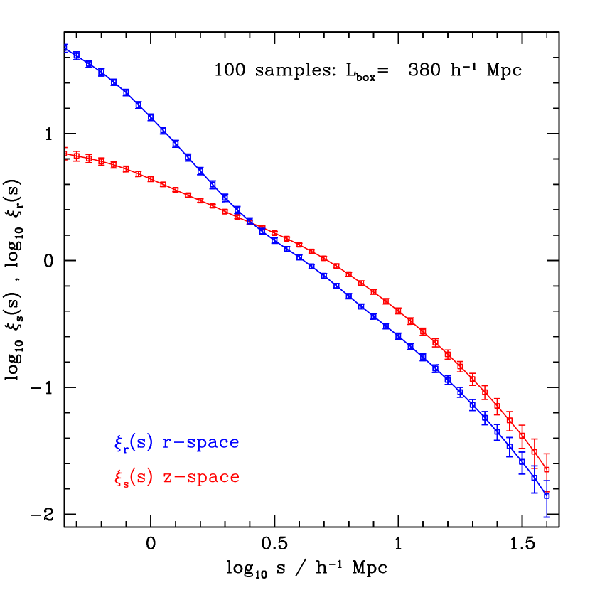
We present results for the projected correlation function and the spherically averaged correlation functions in both real and redshift space. Selected results later on in the Section depend on the number of bins used to represent the correlation function. In most plots we focus on the scales $1.0\lesssim r/{\,h^{-1}\,{\rm Mpc}}\lesssim 25$ for the following reasons. First, this range is accurately modelled in the L-BASICC simulations, and can be measured reliably within all of the sub-volumes the data sets are split into. Second, the model fitting presented in Section 5 is only valid down to $\sim 1.0~{}{\,h^{-1}\,{\rm Mpc}}$, and it therefore makes sense to present other results over the same range of scales for comparison. Third, this range is the most appropriate to draw direct analogies with more general analyses of the error in galaxy clustering measurements. On sub-Mpc scales the precise way that galaxies are distributed within their host halo strongly influences the correlation function and its error. In real-space, scales larger than $\sim 20~{}{\,h^{-1}\,{\rm Mpc}}$ are even more problematic as estimates can be affected by systematics at the $\sim 30$ % level (see Fig. 1), if special care is not taken when accounting for redshift space distortions. Fourth, this choice of scale produces clustering estimates that can be split into sufficiently small but still well sampled bins.

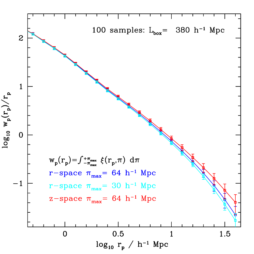
We first present measurements of the basic correlation functions we will be working with throughout the remainder of the paper. Fig. 1 shows the spherically averaged correlation functions, $\xi_{r}(s)$ and $\xi_{s}(s)$, and the projected correlation function, w_p(r_p)/r_p, in the left and right panels respectively, as estimated from the 100 independent data sets of $380~{}{\,h^{-1}\,{\rm Mpc}}$ aside. In the left panel of Fig. 1, we see the clear impact of redshift space distortions on the measured $\xi_{s}(s)$. On small scales, the clustering signal is severely damped by the peculiar motions of the dark matter particles (responsible for the fingers-of-God due to cluster-mass haloes in a $\xi_{s}(r_{\rm p},\pi)$ representation). On intermediate scales, large scale infall enhances the clustering amplitude compared with the real space measurement (see Peacock & Dodds 1994 for a model of the small and large scale redshift space distortion). $\xi_{r}(s)$ shows the well known shoulder between 1 and $3~{}{\,h^{-1}\,{\rm Mpc}}$ (Zehavi et al. 2004), a sign of the transition between the one and two halo terms used in halo occupation distribution models (e.g. Berlind et al. 2003).

Figure 2: The mean relative variance of $\xi_{r}(s)$ (left), $\xi_{s}(s)$ (middle) and w_p(r_p) (right) as a function of scale for different error estimators: black – 100 “mock” data sets; red – two different samples of the mocks (the first 50 & the last 50); green – bootstrap errors after splitting each data set into 27 sub-samples (i.e. Boot-27 with $N_{r}$=$N_{sub}$); blue and cyan – jackknife errors measured after splitting each data set into 27 and 64 sub-samples respectively (i.e. Jack-27 and Jack-64). See §4.2 for comments.

In the right hand panel of Fig. 1 we show the projected correlation functions, w_p(r_p)/r_p, in real and redshift space. By real-space, here we mean that we integrate over an estimate of $\xi_{r}(r_{\rm p},\pi)$ made without including peculiar motions. The comparison between these results illustrates the sensitivity of the projected correlation function to the choice of $\pi_{\rm max}$ in Eq. 8. Theoretically, if one integrates out to $\pi_{\rm max}=\infty$, Eq. 8 would return a purely real space quantity. For numerical as well as computational reasons we restrict the integration to $\pi_{\rm max}\leq 64~{}{\,h^{-1}\,{\rm Mpc}}$. Even at $r_{\rm p}\sim 10~{}{\,h^{-1}\,{\rm Mpc}}$ there is a systematic difference of 10 % in this case between w_p(r_p)/r_p estimated for data in real and redshift space. This difference increases with scale, and by $\sim 30~{}{\,h^{-1}\,{\rm Mpc}}$ it is greater than 50 %. Due to the large sub-volumes used this systematic effect is statistically non-negligible. Taking the individual errorbars at face value (which we show below to be ill-advised), at $\sim 20~{}{\,h^{-1}\,{\rm Mpc}}$ this difference is about 1-$\sigma$. For comparison purposes, we plot w_p(r_p)/r_p estimated in real space data using $\pi_{\rm max}=30~{}{\,h^{-1}\,{\rm Mpc}}$ (cyan). Even in real space, the chosen value of $\pi_{\rm max}$ has non-negligible consequences.

The fact that the real and redshift space measurements of the projected correlation function do not perfectly agree in the right hand panel of Fig. 1 has important implications for the interpretation of w_p(r_p). An estimate of the projected correlation function made from data in redshift space will still be influenced by the underlying redshift space distortions if the integral is not performed out to large enough scales. In our analysis, the magnitude of the systematic shifts is calculated for simulated cold dark matter particles. In the case of real galaxies, some of which are strongly biased with respect to the underlying dark matter, the discrepancy could be even larger. One should therefore be cautious about considering w_p(r_p) as a “real space” measurement, and take even more care in understanding the effect of the limiting $\pi_{\rm max}$ value.

4.2 Mean relative variance as function of scale

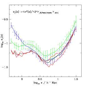
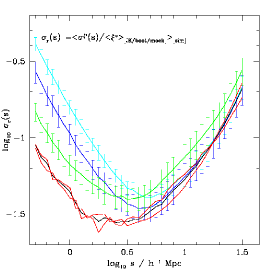
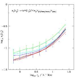
In Fig. 2 we present the mean relative variance of $\xi_{r}(s)$ (left), $\xi_{s}(s)$ (centre) and w_p(r_p) (right), all as function of scale for different error estimators. The mean relative variance for each statistic is defined in the top left corner of each panel.

The relative variance on the clustering measurements estimated from the scatter over the 100 data sets is robust (solid black). If we consider the first 50 and last 50 data sets as separate ensembles (solid red), we find very similar results for the relative variance. However, for all three statistics considered ($\xi_{r}(s)$, $\xi_{s}(s)$ and w_p(r_p)), neither the bootstrap nor jackknife is able to fully recover the relative variance of the mocks as function of scale. Bootstrap estimates for which the number of sub-volumes selected, $N_{r}$, is equal to $N_{sub}$ tend to systematically overestimate the relative variance by 40-50 % on all scales. Jackknife estimates show a scale and statistic dependent bias, varying from no bias on scales larger than $\sim 10~{}{\,h^{-1}\,{\rm Mpc}}$, to a 25 % overestimate for w_p(r_p), and as much as 200 to 400 % for $\xi_{r}(s)$ and $\xi_{s}(s)$ on sub-Mpc scales. We have checked that these differences are not due to a systematic uncertainty in the recovered mean of each statistic: even when rescaling the variance by a simple power-law, the conclusions remain unchanged.

Figure 3: The distribution of projected correlation function measurements for different estimators: left: mock, centre: jackknife and right: bootstrap. We plot the distribution of the $\log_{10}$ of the measurement divided by the mean for that scale; different colours show the distributions for different scales, as indicated by the legend on each panel. In the case of the mocks, the mean is the average over the 100 data sets. For the jackknife and bootstrap, the mean is averaged over the resamplings of each data set. The dotted lines show the corresponding Gaussian distribution, with same mean and variance, the latter indicated on the right in each panel. In this plot, we show results for the jackknife and bootstrap for data sets divided up into 27 sub-volumes.

A closer look at the data set copies generated here with the bootstrap method reveals that the mean effective volume of the copies is only $\sim 63\%$ of the volume of the original data set (i.e. in the case where the number of sub-samples selected at random with replacement equals the number of sub-samples the data set is divided into, $N_{r}$=$N_{sub}$). Perhaps somewhat surprisingly, this value for the mean effective volume depends only weakly on the number of sub-volumes into which the original data set is divided: in fact, for a data set split into a large enough number of sub-volumes the mean is insensitive to the exact $N_{sub}$ value. This reduction in effective volume could, in principle, explain why the mean relative variance is systematically larger for the bootstrap than that expected from the mocks. To increase the effective volume of the bootstrap copy, we need to sample more sub-volumes, i.e. oversample the number of sub-volumes w.r.t. the standard case $N_{r}$=$N_{sub}$. We have experimented with oversampling the number of sub-volumes 2, 3 and 4 times (lower half of Table 1). As expected, the mean relative effective volume does tend then towards unity: for $N_{r}$ = 2 $N_{sub}$, 3 $N_{sub}$ and 4 $N_{sub}$, the mean relative effective volumes are $\sim~{}87\%$, $\sim~{}95\%$ and $\sim~{}98\%$ respectively. The effect of this on the mean relative variance is discussed further in §5.5.

The shapes of the relative variance computed using the different methods are different as a function of scale. While $\sigma_{r}$ for $\xi_{r}(s)$ and $\xi_{s}(s)$ show a clear minimum between 3-6 and 2-3${\,h^{-1}\,{\rm Mpc}}$ respectively, $\sigma_{r}$ for w_p(r_p) shows no evidence for an increase in the relative variance on moving to the smallest scales considered. This dependence could be related to the number density of dark matter particles used in the analysis, with $\xi_{r}(s)$ and $\xi_{s}(s)$ being maybe more sensitive to Poisson noise on small scales than the integral statistic w_p(r_p). The flattening in the relative variance seen in the mocks for $\xi_{r}(s)$ corresponds to the scale where the dominant contribution to the correlation function changes from the one-halo term (small scales) to the two-halo term.

It is important to remember that it is not possible from Fig. 2 alone to quantify the inevitable correlations between different scales in the clustering statistic. It would be naive to assume that these are unimportant, but let us here for simplicity consider that naive situation of uncorrelated errors. In the case of jackknife errors, the different scale dependence of the relative variance (compared with the “truth”) makes their interpretation more complicated and therefore more likely to lead to misleading conclusions, especially if the small scale clustering is included. On the positive side, the jackknife errors, as presented here, tend to overestimate the true errors, which is certainly better than underestimating them. In the case of the bootstrap errors, on the other hand, the relative variance as a function of scale has a similar shape to that of the variance from the mocks, and so the variance could be rescale by an appropriate factor to take into account the overall overestimate of the relative variance. As with jackknife errors, the bootstrap errors, as presented here, do not underestimate the errors on any of the scales considered, which is a good thing if one is to consider an uncorrelated error analysis.

4.3 Distribution of correlation function measurements

Having compared the estimates of the relative variance of the correlation function in the previous section, let us now look at the distributions of the measurements of the correlation functions themselves. The motivation for doing this is clear. Recall that in order to be able to interpret $\chi^{2}$ fitting in the standard way, assigning the confidence intervals associated with a Gaussian distribution to set differences in $\chi^{2}$, we need to find a quantity which is Gaussian distributed to use in the fitting process.

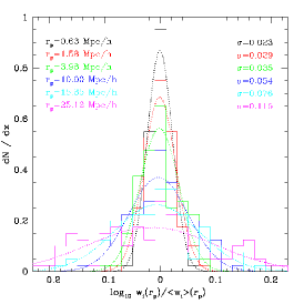
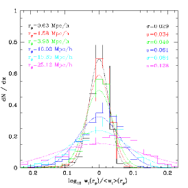
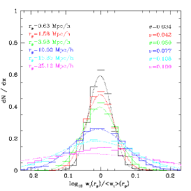
The distribution of the measured projected correlation functions are compared in Fig. 3. Each panel corresponds to a different error estimation method (left: mocks; centre: jackknife; right:bootstrap). We plot the $\log_{10}$ of the measured projected correlation function divided by the mean value, which shows deviations on either side of the mean on an equal footing. The different histograms show the distributions of $\log_{10}$ w_p(r_p)/$<$w_p(r_p)$>$ measured on different scales covering the range $0.60$ to $25~{}{\,h^{-1}\,{\rm Mpc}}$. The dotted curves show the corresponding Gaussian distributions, i.e. with same mean and variance.

A quick comparison of the shapes of the histograms in the different panels shows that the distribution of $\log_{10}$ w_p(r_p)/$<$w_p(r_p)$>$ appear Gaussian for all estimates on small scales, while on larger scales, this is no longer true for jackknife and bootstrap estimates ($r_{p}\gtrsim 5~{}{\,h^{-1}\,{\rm Mpc}}$ and $r_{p}\gtrsim 15~{}{\,h^{-1}\,{\rm Mpc}}$ respectively). On the largest scales considered here, even the distribution from the mocks seems to be boarder than its corresponding Gaussian equivalent. The distributions yielded from the jackknife estimator tend to show asymmetry on most scales plotted. Thus, despite these deviations from a Gaussian distribution, we conclude that $\log_{10}$ w_p(r_p) is closer to being Gaussian than w_p(r_p) is, and, as such, is a more appropriate choice of variable to use in a $\chi^{2}$ fitting.

Figure 4: Left : The normalized eigenvalues (i.e. normalized relative variance contributions) for the redshift space correlation function, $\xi_{s}(s)$, as function of eigenvalue number. The black line shows the eigenvalues for 100 mock data sets, while the two red lines correspond to the eigenvalues obtained from the covariance matrix obtained using the first and last 50 mocks only. As in Fig. 2, this illustrates the scatter in the mock eigenvalues. The green line shows the equivalent result for the Boot-27 errors, while the blue and cyan lines show the Jack-27 and Jack-64 errors respectively. Errorbars indicate the 1-$\sigma$ scatter on applying the error estimates to the 100 data sets. The range of pair separations considered in the principal component decomposition is given in each panel. Right: Same as left panel but for the projected correlation function, w_p(r_p), estimated from the simulations put into redshift space.

The middle panel of Fig. 3 shows the distribution of the jackknife w_p(r_p) estimates. Note that, as a result of the method of construction, jackknife errors are much more highly correlated than all the others, which is reflected by the additional factor of $N-1$ in the numerator of the expression for the covariance matrix (Eq. 2). Hence, to compare the jackknife distribution with the others, we first need to rescale the ratio w_p(r_p) by $\rm\sqrt{N_{sub}-1}$. Similarly, it is essential to account for this factor when plotting jackknife errorbars on data points, as otherwise they do not correspond to the variance in the jackknife estimates. A quick comparison of the middle and left panels in Fig. 3 shows that the distribution of jackknife estimates over this medium range of scales is similar to the corresponding mock distribution: the jackknife distribution is slightly wider than the mock on small scales, which agrees with the comparisons of the variances presented in §4.2. However, this figure also shows a concerning trend in that the jackknife distribution tends to become more asymmetric on larger scales ($r_{p}\gtrsim 10~{}{\,h^{-1}\,{\rm Mpc}}$), implying that jackknife errors for $\log_{10}$ w_p(r_p) are not Gaussianly distributed on such scales.

Finally, in the right panel of Fig. 3 we show the distribution of bootstrap w_p(r_p) measurements. On all scales considered the distribution is clearly wider than that obtained from the mocks. This highlights the fact that, when only considering the diagonal terms from the covariance matrix (as is commonly done), bootstrap errors are generally larger than both mock and jackknife errors, as was clear from §4.2 already. However, this does not necessarily mean that bootstrap errors overestimate the uncertainty, as we need to take into account the correlation between errors as well. Clearly, in an analysis which ignores the correlation of the errors, the errorbars will be overestimated using the bootstrap method. It should be stressed that the values of $\log_{10}$ w_p(r_p) obtained from the bootstrap, unlike those from the jackknife, are certainly more Gaussianly distributed, with perhaps some hint of a non-Gaussian error distribution appearing only for $r_{p}\gtrsim 25$.

4.4 Eigenvalues

So far we have ignored any correlations between bins when presenting the errors. To correct for this omission, we now consider the first step in a principal component decomposition of the covariance matrix, the distribution of normalized eigenvalues. The normalized eigenvalues quantify the contribution to the variance of the corresponding eigenvector.

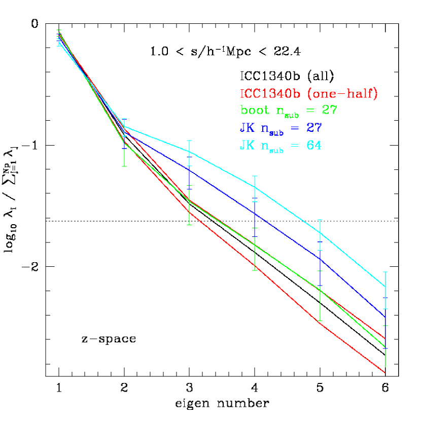
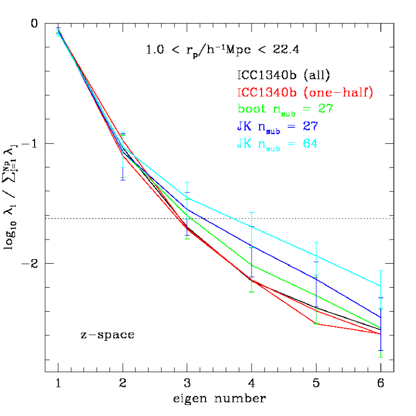
In the two panels of Fig. 4 we present the normalized eigenvalues for the covariance matrix of redshift space correlation function measurements, $\xi_{s}(s)$ (left), and for the projected correlation function, w_p(r_p)/r_p (right), in both cases as function of eigenvalue number. The eigenvalues are ranked in order of decreasing variance, with the first eigenvalue accounting for the largest variance. The results in this plot are dependent on the number of data points used. In this case, the correlation functions are estimated in logarithmic bins of pair separation with width of 0.2 dex.

In each panel, the black line corresponds to the mock eigenvalues (which we call the “truth”), and the red lines indicate the eigenvalues obtained from the covariance matrix constructed using just one half of all the mock realizations. This provides an indication of the accuracy with which the mock eigenvalues are measured. Interestingly, the accuracy of the eigenvalues in this test is higher for w_p(r_p)/r_p (right) than it is for $\xi_{s}(s)$ (left). This is most likely related to the fact that, within the range of scales considered, $\xi_{s}(s)$ is more sensitive to Poisson noise than w_p(r_p)/r_p, as was the case for the results in Section 4.2.

Fig. 4 shows that in all cases, the eigenvalues decrease strongly in amplitude with increasing eigennumber. The first two eigenvalues alone typically account for 80 or even 90 % of the total variance. This indicates that a very strong correlation exists between the bins in the correlation function measurements. The shape of each eigenvalue curve is dependent on the correlation function itself. Somewhat surprisingly, $\xi_{s}(s)$ appears to be a less correlated statistic than w_p(r_p)/r_p, as more eigenvalues are needed in the former case to represent the covariance matrix with the same level of fidelity i.e. to the same total variance. Or, in other words, the eigenvalue curve is shallower for $\xi_{s}(s)$ than it is for w_p(r_p)/r_p. Changing the range of scales or the number of data points used to represent the correlation function has only a marginal impact on the form of the eigenvalue curves.

Eigenvalues derived from the bootstrap covariance matrix are shown by the green line in each panel of Fig. 4, with error bars indicating the scatter over the 100 mock data sets. Here we show only the bootstrap eigenvalues obtained using 27 sub-volumes. On average, the bootstrap method recovers the expected eigenvalue curve rather accurately. Although it is not a perfect match, the “truth” (i.e. mock) is always within the scatter presented for both clustering statistics. Note that changing the scale or the number of data points considered does not appear to influence these conclusions.

The eigenvalues obtained from the jackknife covariance matrix are shown in Fig. 4 for two choices for the number of sub-volumes, 27 and 64, shown by the blue and cyan lines respectively. Once again, error bars indicate the scatter in the eigenvalues obtained by applying this technique to each of the 100 data sets. Neither of the two jackknife measurements fully recovers the true eigenvalues. Interestingly, the more sub-samples that are used, the further away the eigenvalue curves move from the “truth”. For $\xi_{s}(s)$, this appears to be mostly due to the much smaller first eigenvalue, which is $\sim 0.6\pm 0.1$ instead of $\sim 0.85\pm 0.1$. Furthermore, the slope of the eigenvalue curve is different than that obtained from the mock data sets and is very sensitive to the number of sub-volumes the data is divided into. We have checked that further increasing the number of sub-samples the data is split into simply exacerbates this problem. This is a first yet clear indication that the covariance matrix estimated from the jackknife technique is not equivalent to the “correct” mock estimate. However, these issues do not necessarily imply that the jackknife error estimate is incorrect, since the eigenvalues are just one part of the principal component decomposition. On the other hand, this highlights the limitation in how accurately the jackknife methodology can recreate the true underlying errors, as given here by the mocks. Most of the above remarks remain true for w_p(r_p)/r_p as well. As was the case with the bootstrap analysis, changing the scale or the number of data points does not significantly influence any of the above conclusions.

Figure 5: Left: The normalized eigenvectors for the spherically averaged redshift-space correlation function, $\xi(s)$, as function of scale. Each panel corresponds to a different eigenvector, whose contribution to the total variance (in the mock case) is indicated on each panel. Colour and line styles are the same as in Fig. 4. Error bars show the 1-$\sigma$ scatter obtained from the 100 data sets. The range of physical scales considered in the principal component decomposition is indicated in the legend. Right: Same as left panel, but for the projected correlation function, w_p(r_p)/r_p, as function of projected separation.

4.5 Eigenvectors

After considering the eigenvalues of the principal component decomposition we now examine the associated eigenvectors. Together, the eigenvalues and eigenvectors completely describe the full normalized covariance matrix.

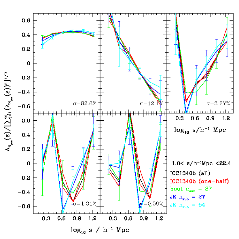
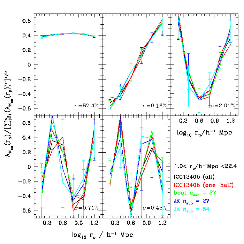
In Fig. 5, we show the first five eigenvectors derived from the covariance matrices constructed for the spherically averaged correlation function ($\xi_{s}(s)$, left), and for the projected correlation function (w_p(r_p)/r_p, right). Note these eigenvectors are in the same order as the eigenvalues presented in Fig. 4. Only the eigenvector corresponding to the smallest eigenvalue is not shown, which contributes less than $\approx 0.3$ % to the total variance. The colour coding remains the same as that used in Fig. 4, with the contribution to the relative variance indicated in the bottom right corner of each panel. At first sight, the results are rather encouraging, as the mean eigenvectors for all error calculation methods overlap reasonably well with that measured from the mocks (the “truth”, shown by the black line). The scatter on the mock result is indicated by the spread between the red lines, which, as before, shows the results obtained from splitting the mock data sets into two groups of 50.

Let us consider each eigenvector for both $\xi_{s}(s)$ and w_p(r_p)/r_p more carefully. The first and most important eigenvector (top left corner of both panels in Fig. 5) is very flat and is related to the uncertainty in the mean density of objects in the data sets. This uncertainty causes all the clustering measurements to move up and down more or less coherently. To within the quoted scatter on each clustering measurement, all of the first-ranked eigenvectors are identical. However, some interesting trends can already be seen in this decomposition. For example, increasing the number of sub-samples used from 8 to 27 increases the difference between the mock and jackknife estimates, with the shape of the data inferred eigenvector tending to show less (more) correlation on small (larger) scales. This is a real effect that is further enhanced as one considers even smaller scales than shown here.

The second eigenvector in Fig. 5, shown in the top middle row of both panels, displays a strong scale dependence unlike the first eigenvector. The second eigenvector gives a much smaller contribution to the total variance, i.e. around the $\sim 10$ % level, as opposed to $\sim 85$ % for the first eigenvector. The form of the second eigenvector reveals that small scales are anti-correlated with larger ones. It is worth noting that all three error methods yield eigenvectors which look very similar for both $\xi_{s}(s)$ and w_p(r_p)/r_p. Increasing the number of sub-volumes decreases slightly the scatter in the recovered second eigenvector, and for a fixed number of sub-samples the scatter is marginally smaller for the bootstrap error estimates. Finally, it is worth noting that the correlations as function of scale, despite having different slopes for $\xi_{s}(s)$ and w_p(r_p)/r_p, are in fact very similar: the orientation of the eigenvectors is only determined up to a sign, so all the curves in Fig. 5 can be arbitrarily multiplied by -1.

The remaining three eigenvectors plotted in Fig. 5 combined contribute less than a few percent of the total variance, and the smaller their contribution to the variance, the larger is the scatter from the different resamplings. The fifth eigenvector (bottom right panel) certainly tends to be dominated by point to point variations in the data itself. This behaviour is particularly obvious when most of the eigenvector signal appears to come from adjacent points with opposite correlations, as seen in the lower panels for both statistics.

Note that it is precisely this last point, whether or not the eigenvector provides a useful or important description of the data, that highlights the difficulty behind using a principal component analysis. When fitting a model to the data, we need to select how many principal components to use in the fit (see the example in Section 5). If features in the data are real then any theoretical model should attempt to reproduce them, and the eigenvectors which encode these features should be retained. However, if any facet of the data is dominated by noise then we should not attempt to reproduce it, and we should omit the corresponding eigenvector. One can compare covariance matrices without worrying about whether or not to retain different eigenvector components; however, this issue has a major bearing on the success of model fitting.

4.6 Stability of (inverted) covariance matrices

So far we have compared the principal component decomposition of covariance matrices constructed using different techniques to what we know is the “right” answer - the covariance matrix obtained from a set of mock data sets. Unfortunately, in practice, it is rarely the case that one knows the correct answer beforehand. It would be useful, therefore, to devise a statistic which will allow us to quantify the degree to which a given technique can recover a covariance matrix. Clearly no statistic can ever know the precision to which a measurement is actually correct, since that would require a priori knowledge of the “truth”. But the statistic should at least be sensitive to the level of noise which remains in the covariance matrix estimate. In the absence of such a statistic at present, we consider the usefulness of a few well-known results on the stability of errors in our quest to determine the stability of the inversion of the covariance matrix.

One of the easiest tests to check the stability of a covariance matrix inversion is to repeat the whole analysis using only the odd or even data points (i.e. the 1st, 3rd, 5th … data points), and to check that the results remain within the quoted errors, and, furthermore, that no systematic shift has been introduced in either case. Similarly, the result should remain stable to a simple rebinning of the data. Note that the rebinning should be done at the level of the data itself and not on the processed results. This is to ensure that non-linearities in the binning procedure do not introduce unwanted biases. In the case of 2-point clustering statistics, this means that pair counts should be rebinned.

Porciani & Norberg (2006) considered a quantitative test for the bootstrap method, which consists of using $\chi^{2}$ values in order to assess the stability of the recovered covariance matrix. Their method relies on quantifying how many components of the principal component decomposition can be reconstructed for a fixed number of bootstrap realizations. The figure of merit is obtained by comparing the $\chi^{2}$ distributions for two different sets and numbers of bootstrap samples, as a function of the number of principal components used. With this method, it is possible to at least make sure that the number of bootstrap realizations is large enough, but under no circumstance can we tell whether the method chosen has converged to the “true” covariance matrix. One nice feature of the method is that it can actually show that certain components of the decomposition will under no circumstance be recovered accurately enough, in which case this gives an indication of how many components should actually be considered.

Last but not least, the results should be stable w.r.t. the number of sub-samples considered (within moderation of course). This is something which has to be considered in both bootstrap and jackknife analyses, and remains probably one of the better ways to at least attempt to show that the results obtained with internal errors estimates are as accurate and realistic as possible.

In Section 5, we put the above remarks into practice and show that each of them are able to fix or highlight different and often problematic issues in the error analysis using internal estimates. We note here that it is due to the numerous mock realizations that we are actually able to discover, on a more rapid timescale, which of the different methods is the more promising. Certainly the task would be much more difficult in their absence.

Figure 6: Left: The projected dark matter correlation function, estimated from a set of non-linear power spectra with $\Omega_{0}=0.25$ and $0.30\leq\sigma_{8}\leq 2.00$, in steps of $\delta\sigma_{8}=0.02$ (see text for details). Like the results presented in Section 4.1, the projected correlation functions are calculated at $z=0.50$. Right: The same as the left panel, but now assuming $\sigma_{8}=0.90$ and $0.05\leq\Omega_{0}\leq 0.99$, in steps of $\delta\Omega_{0}=0.02$ (see text for details).

5 A case study: cosmological parameter estimation

In this section we illustrate the different error estimation methods introduced and discussed in Sections 2 and 4 with a case study involving the projected correlation function. The aim is to infer two basic cosmological parameters, the matter density, $\Omega_{0}$, and the amplitude of density fluctuations, $\sigma_{8}$, using measurements of the projected correlation function made from the mock data sets between 1 and $\sim 22~{}{\,h^{-1}\,{\rm Mpc}}$. In this example, because we are using data sets extracted from N-body simulations, we know the true values of the parameters beforehand, and can therefore test the performance of the error estimators.

5.1 A grid of theoretical w_p(r_p) models

We first describe how to compute a grid of models for the projected correlation function using linear perturbation theory. First, we construct a grid of linear perturbation theory power spectra, using the parameterization of the cold dark matter transfer function introduced by Eisenstein & Hu (1998). This parameterization is an approximation to the more accurate results generated from Boltzmann codes such as CAMB (Lewis & Challinor 2002; see Sanchez et al. 2008 for a comparison). The initial conditions for the L-BASICC simulations were computed using CAMB, so we would expect a small systematic error in the values of the recovered cosmological errors. However, for this application, the measurement errors are much larger than these systematic errors, and we use the Eisenstein & Hu (1998) equations for speed and simplicity.

The parameters varied to construct the grid are the normalization of the power spectrum, $\sigma_{8}$ (over a range $=0.3$ to $2.0$ in steps of 0.02) and the present day matter density parameter $\Omega_{0}$ (covering the range $=0.05$ to $1$ in steps of 0.02). The other cosmological parameters are held fixed at the values used in the simulation, as described in Section 3.1. The power spectra are output at $z=0.5$ to match the redshift of the simulation output. The next step is to produce an approximate estimate of the non-linear matter power spectrum, using the HALOFIT code of Smith et al. (2003), which has been calibrated against the results of N-body simulations. Finally, we transform the power spectrum into the projected correlation function. The relation between the real-space correlation function, $\xi_{r}(r)$, and the projected correlation function is well known:

$$\frac{w_{\rm p}(r_{\rm p})}{r_{\rm p}} = \frac{2}{r_{\rm p}}\int_{r_{\rm p}}^{\sqrt{r_{\rm p}^{2}+\pi_{\rm max}^{2}}}\xi_{r}(r)\frac{r}{\sqrt{r^{2}-r_{\rm p}^{2}}}{\rm d}r~{}.$$ (14)

Using the fact that the power spectrum is the Fourier transform of the correlation function, we can replace $\xi_{r}(r)$ to obtain, in the limit that $\pi_{\rm max}\rightarrow\infty$:

$$\frac{w_{\rm p}(r_{\rm p})}{r_{\rm p}} = \frac{1}{2\pi r_{\rm p}}\int_{0}^{\infty}kP(k)J_{0}(kr_{\rm p}){\rm d}\ln k~{}.$$ (15)

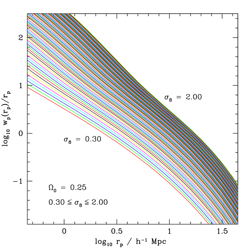
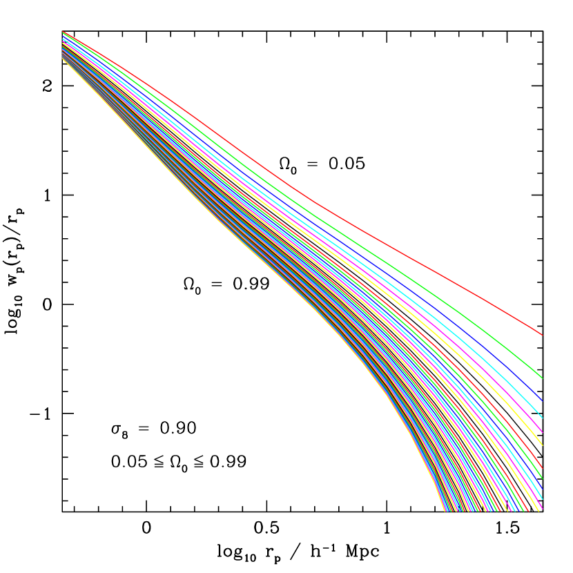
Note that if a finite value of $\pi_{\rm max}$ is used to obtain the measured projected correlation function, then strictly speaking, $J_{0}$ in Eq. 15 should be replaced by a finite integral over $\sin(kr)/(kr)$. Instead we correct for the small systematic error introduced by retaining $\pi_{\rm max}\rightarrow\infty$ by forcing the theoretical prediction for $\Omega_{0}=0.25$ and $\sigma_{8}=0.9$ to agree with the measurement from the full simulation volume; this correction is applied to all the projected correlation functions on the grid and works well, which is clear since the returned best fitted values are still centred on the expected values. The dependence of the projected two-point correlation function on $\Omega_{0}$ and $\sigma_{8}$ is illustrated in Fig. 6. The left hand panel shows the dependence of w_p(r_p)/r_p on $\sigma_{8}$ for $\Omega_{0}$ fixed to the value used in the L-BASICC simulation, while the right hand panel shows the dependence on $\Omega_{0}$ with $\sigma_{8}$ fixed to the simulation value.

Figure 7: $\Delta\chi^{2}=6.17$ contours (i.e. 95 % confidence interval for a 2-parameter fit in the case of Gaussian distributed errors) in the $\Omega_{0}$-$\sigma_{8}$ plane, for three hundred and one error estimates. The most realistic error estimate is given by the mock errors (thick black), while red (dotted) correspond to bootstrap errors with 27 sub-samples, blue (short dashed) to jackknife with 27 sub-samples and cyan (long dashed) to jackknife with 64 sub-samples. From this rather ‘messy’ plot, it is clear that internal error methods do not necessarily return the correct errors. The fits projection correlation function fits are done over the scales indicated in the legend.

5.2 A straightforward 2-parameter model fitting?

Armed with our grid of theoretical models we are now ready to test the internal error estimators against the external estimate, the mocks, which we regard as the “truth”. We note that this is an idealized case, which is perfect for assessing the performance of the internal estimators: we know the true values of the cosmological parameters and we know that our model should provide a very good description of the measurements, at least over the range of scales used in the fit. In a more realistic situation, the complications of galaxy bias, sample selection and how well we could model these effects would have an impact on performance (see for example Angulo et al. 2008).

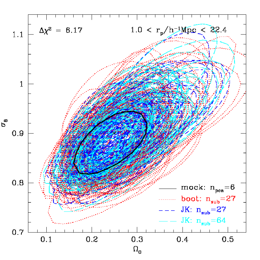
As this is such a straightforward fitting problem, we choose in Fig. 7 to plot the raw 95 % confidence interval contours in the $\Omega_{0}$-$\sigma_{8}$ plane for three hundred and one error estimates. Remember that in a normal situation with 1 data set, we would only be able to obtain three estimates of the error, whereas in our case we have 100 data sets and can therefore study the distribution of internal error estimates. The black solid contour corresponds to the 95 % confidence interval inferred from the mocks, which we consider as the “truth” or the benchmark error that the other methods are trying to match. The red-dotted lines correspond to Boot-27 (with $N_{r}$=$N_{sub}$), blue-short dashed to Jack-27 and cyan-long dashed to Jack-64. The rather messy nature of this plot tells us that there is little agreement between each of the error methods and even between different realizations using the same estimator.

Figure 8: The distribution of the normalized figure of merit, A / A_mock (see §5.2 for details). Boot-27 results are shown in red, Jack-27 and Jack-64 are in blue and cyan respectively. The arrows indicate the median of each distribution, while the dotted curves show the corresponding Gaussian with mean and variance indicated in the panel. In the left (right) panel, the number of principal components used is six (thirteen) out of the six (thirteen) data points used to cover the range of scales considered.

Two generic trends can be seen in Fig. 7. First, not all contours are centred on the true values used in the simulations of $\Omega_{0}=0.25$ and $\sigma_{8}=0.90$, but appear to be systematically shifted around. This is the effect of sample variance, also more commonly (but less correctly) referred to as cosmic variance. Indeed, each data set, despite being very large (a cube of side $380~{}{\,h^{-1}\,{\rm Mpc}}$), is sensitive to the large scale density fluctuations present in the much larger simulation volumes. Irrespective of the error method used, the distributions of best fit $\Omega_{0}$ values are all symmetric, but not exactly Gaussian (the central part being slightly more peaked than a Gaussian with similar dispersion) and with mean values less than a $\delta\Omega_{0}$-binsize away from the simulation value. The distributions of best fit $\sigma_{8}$ values are all very well described by Gaussian distributions, with similar dispersion and with mean values within a $\delta\sigma_{8}$-binsize from the ICC1340 simulation value. Second, some of the error contours from the internal estimators are much larger than the mock error contour, while others are clearly much smaller. This, on the other hand, is of concern for internal error estimates and merits therefore closer investigation.

To further quantify the conclusions drawn from Fig. 7, we construct a relative area statistic, defined as the area encompassing the 95 % confidence interval in an internal error estimator divided by the area of the external, “true” mock error estimate, A / A_mock, for the same number of principal components. The motivation behind this statistic, hereafter also referred to as the normalized figure of merit, is twofold: 1) for a 2 parameter model it is natural to make comparisons between different error estimators using the full parameter plane; and 2) due to its dimensionless nature, this statistic is easily interpreted in terms of confidence levels (see below). A drawback of this figure of merit is that it does not account for uncertainties in the determination of the mock area/contours, which, given the number of data sets available, can not be neglected. A zeroth order estimate of that effect is given by a comparison between the following three mock results: those obtained using all 100 mocks, the first 50 and the last 50 respectively. Additionally, it is not possible to estimate this statistic for real data, but only for slight variants of it.

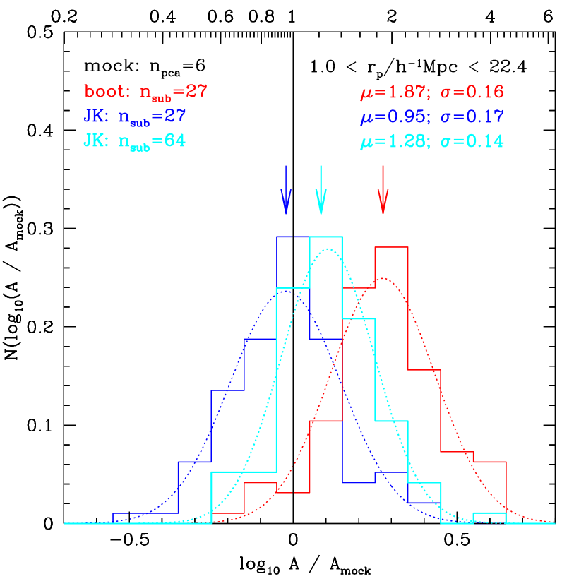
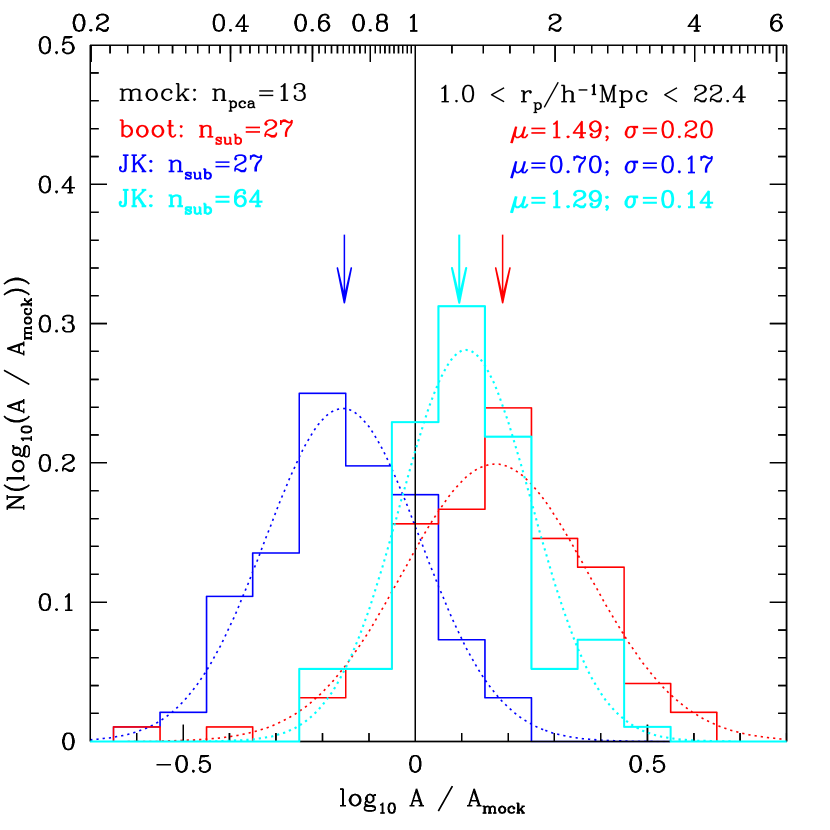
In Fig. 8 we plot the distribution of the relative area statistic. The case of Boot-27 (with $N_{r}$=$N_{sub}$) is shown in red, results for Jack-27 and Jack-64 are shown in blue and cyan respectively, while the black vertical line indicates the optimal value of the mock. The arrows show the median of each distribution. The difference between the two panels is the binning used for w_p(r_p)/r_p, and hence, indirectly, in the number of principal components considered.

Focusing on the left panel of Fig. 8 first, we see that for most data sets, the internal error estimates (of which three hundred are presented in this figure) tend to overestimate the 95 % CI area, on average by factors of $\sim 1.9$, $\sim 1.3$ and $\sim 0.95$ for Boot-27, Jack-64 and Jack-27 respectively. Furthermore, the variation in the area of the error contours is substantial: the central 68 % of values is typically spread over 0.15 in log₁₀ A / A_mock, i.e. a factor of $\sim 1.4$ in the area of the error contour. Hence, even for this particularly simple case, the uncertainty on the internal estimate of the CI is large and certainly not negligible. As seen in earlier cases, the difference between Jack-27 and Jack-64 is also quite large, with Jack-64 yielding a marginally more centrally concentrated distribution than Jack-27, whereas Jack-64, on average, overestimates the true area by an additional 30 %. The situation is clearly worst for bootstrap errors, which display by far the largest systematic offset, but with a spread that looks amazingly similar to jackknife results. Interpreting these offsets in the framework of Gaussian errors for this figure of merit, we conclude that on average a 95 % boot-27 CI corresponds effectively to a 99.6 % CI, a 95 % Jack-64 to a 98.0 % CI, and a 95 % Jack-27 CI to a $\sim$90 % CI. This is without taking into account the spread in relative areas from different realizations.

Unfortunately, this is not the end of the confidence interval story. We now consider the right hand panel of Fig. 8, which is equivalent to the left except that 13 bins instead of 6 have been used for w_p(r_p)/r_p (over the same range of scales) and hence all 13 principal components are used in the fitting, instead of just 6 as in the left panel. The difference in the figure of merit between right and left panels is clear, with the offsets of two of the three error methods changing in a systematic way. The right panel area ratios are biased by factors $\sim 1.5$, $\sim 1.3$ and $\sim 0.7$ for Boot-27, Jack-64 and Jack-27 respectively. The only positive note is that all distributions plotted are well described by Gaussians, shown by the dotted lines, with small dispersions. Indirectly, we conclude that on average an estimated 95 % CI corresponds, with 95 % confidence, to a true CI in the range 79.2 % - 99.8 % for the case considered here. We note that only Jack-64 seems to remain stable w.r.t. the change in binning. This is most likely related to the results found by Hartlap et al. (2007). They showed that internal error estimators tend to be systematically biased low on average when the ratio of the number of bins considered to the number of samples becomes too large (typically 20 % or more).

Figure 9: The 16^th, 50^th and 84^th percentiles of the relative area statistic (see §5.2 for a definition) as function of the number of principal components used in the fit: in each case the figure of merit is normalized to the mock area with the same number of principal components. Bootstrap errors from 27 sub-volumes (with $N_{r}$=$N_{sub}$) are shown in red, while jackknife errors are given in blue and cyan for 27 and 64 sub-volumes respectively. In the left (right) panel, six (thirteen) equally spaced data points for w_p(r_p)/r_p are considered in the model fitting and cover the full range of scales indicated in the key. Finally, the black line indicates $\rm A_{\rm mock}^{N_{\rm pca}}/A_{\rm mock}^{N_{\rm ref}}$ with N${}_{\rm ref}=3$ in both panels.

The differences between the distributions of error contour areas shown in the left and right panels of Fig. 8 is disconcerting, since only the number of data points used has changed (i.e. the binning of w_p(r_p)/r_p over a fixed range of scales). For mock errors, we measure an increase of 15 % in the area covered by the 95 % confidence intervals when changing from 6 to 13 data points. This is much smaller than the systematic shifts displayed by the internal error estimates under the same circumstances, which present a 30 % to 80 % change. It is unlikely that these strong shifts are due to the nature of the data alone, but much more likely to be due to errors propagating through the full covariance matrix analysis. In both panels, the fits are performed using the full covariance matrices, and therefore we investigate in the next section if noise in the covariance matrix is the root of the problem.

5.3 Dependence of confidence intervals on N_pca

Perhaps the large variation in the error contours returned by the internal estimators is due to noise in the covariance matrix, resulting from too many principal components being retained in the analysis.

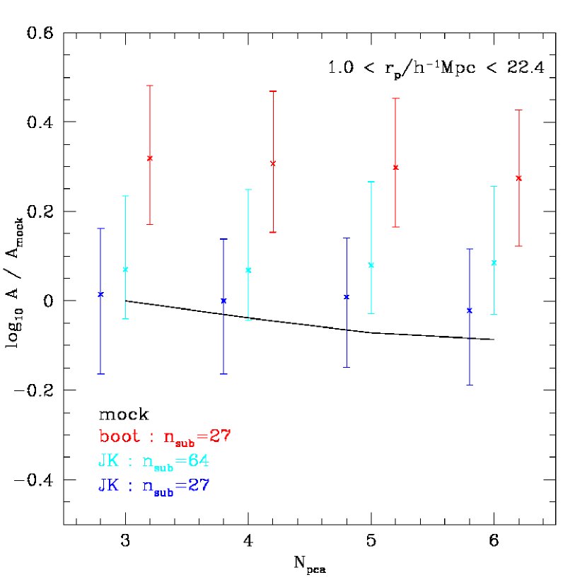
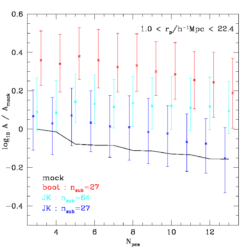
To test this idea, we show in Fig. 9 the impact on the relative area statistic of varying the number of principal components for a fixed number of data points. In the left panel of Fig. 9, 6 data points are used to represent w_p(r_p)/r_p. The variation of the 95 % confidence interval area in the external mock estimate w.r.t. the area with N${}_{\rm pca}=3$ is plotted as a black line. This is a measure of how stable the mock results are as function of the number of principal components. There is a modest reduction in the size of the error contour, $\sim 0.1$dex, on using 6 principal components instead of 3, as shown by the shallow slope of the line. The situation is slightly more unstable in the right panel (where 13 data points are used instead of 6 as in the left panel), with up to a 40 % change over the full range of numbers of principal components considered. This variation is significantly reduced if one starts with at least 5 principal components, where the change in the figure of merit over the full range is then less than $\sim 20$ %.

In Fig. 9 we also show the median, and 16^th and 84^th percentiles of the relative area distributions for Boot-27 (with $N_{r}$=$N_{sub}$), Jack-27 and Jack-64 estimates in red, blue and cyan respectively. The impression gained from the two panels is rather different, especially for Boot-27 and Jack-27. While the main properties of the relative area distributions for those two estimators remain roughly the same as function of N_pca in the left panel (very weak dependence on N_pca), they change systematically and significantly with N_pca in the right panel. These changes result in unstable error estimates, most likely due to the propagation of a bias through the covariance matrix estimate (see Hartlap et al. 2007). Only Jack-64 seems to return a somewhat stable results as function of N_pca.

Finally, in Fig. 10 we examine the fraction of “outlier” experiments as function of the number of principal components used in the fit. An outlier is defined as a data set for which the error contour from an internal estimate (defined by $\Delta\chi^{2}=6.17$) does not include the true underlying cosmology (i.e. $\Omega_{0}=0.25$ and $\sigma_{8}=0.90$). For a Gaussian distribution, we would expect no more than 5 “outliers” defined in this way out of 100 data sets. The left panel looks reasonable for most N_pca, especially considering the number of realizations available: remember we have just 100 data sets at our disposal, so the Poisson noise on the expectation value of this statistic is non-negligible. There is still a tendency from this panel to say that Boot-27 (with $N_{r}$=$N_{sub}$) overestimates the errors and Jack-27 underestimates them. This is in relatively good agreement with our conclusions from Fig. 9. In the right hand panel the situation is significantly different. First all three estimators present radical changes in the number of “outliers” as function of N_pca. Clearly we have to exclude fits which use too many principal components: a cut can therefore be made at about 10 principal components for Boot-27 and Jack-64, while the cut has to be made at about 6 or 7 components for Jack-27 already.

Neither Fig. 9 nor Fig. 10 can be made without the full battery of data sets we have, nor without the knowledge of what the “truth” is. However, we can nevertheless learn some simple tricks which will be useful for the analysis of real data. For example, for each internal error estimator we can plot the relative area statistic, by using a fiducial reference value for the area. If this quantity varies in a significant manner as function of N_pca or as a function of the internal error estimator used, we are made aware of a change of regime, without necessarily knowing what to do. The most likely and robust solution will be to introduce less components in the fit.

Figure 10: The fraction of outliers as function of the number of principal components used in the fit. An outlier is defined as a 2-parameter fit for which the $\Delta\chi^{2}=6.17$ contour of the data inferred errorbar does not enclose the true underlying cosmology, i.e. $\Omega_{0}=0.25$ and $\sigma_{8}=0.90$ (see §3.1). The horizontal line corresponds to the theoretical expectation for the contour $\Delta\chi^{2}=6.17$, i.e. 95 % assuming Gaussianly distributed errors. The left (right) panel corresponds to bins of 0.2 (0.1) dex width.

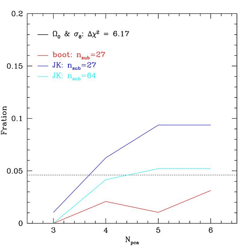
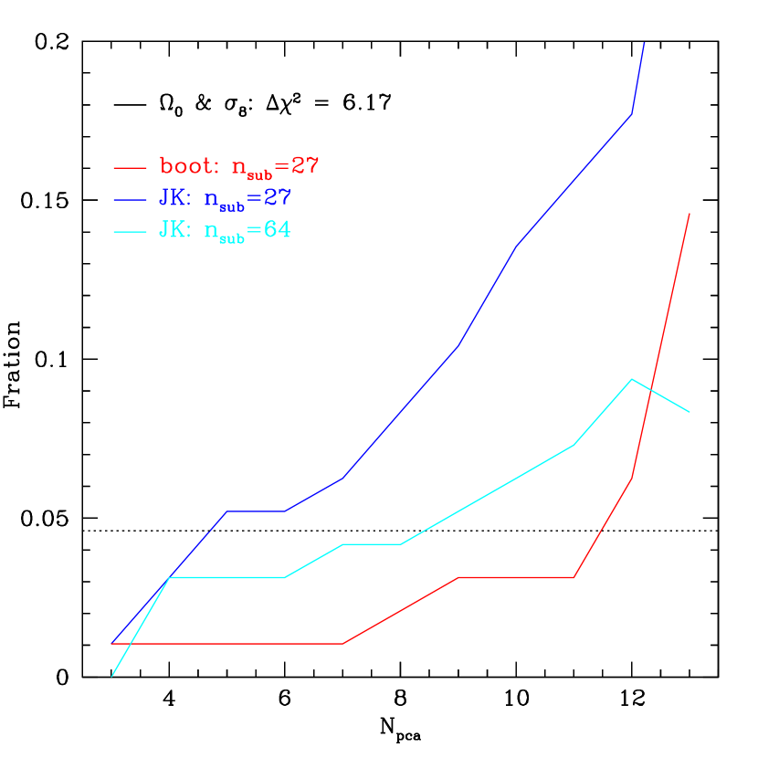
5.4 Important considerations for error analyses

We summarize here a few results from our simple case study. To recap the exercise consisted of fitting the projected correlation function (on scales between 1 and $\sim 22~{}{\,h^{-1}\,{\rm Mpc}}$), using what we knew beforehand was the correct theoretical model and which was only dependent on the parameters $\Omega_{0}$ and $\sigma_{8}$, to one hundred projected correlation function estimates, taken from one hundred data sets of $380~{}{\,h^{-1}\,{\rm Mpc}}$ on a side, extracted from 50 totally independent N-body simulations of $1340~{}{\,h^{-1}\,{\rm Mpc}}$ on a side. The main conclusions for internal error estimates are, with confidence interval abbreviated as CI:

• the average systematic offset encountered on an estimated 2-$\sigma$ CI implies it can be mistaken for a 1.6-$\sigma$ to 2.9-$\sigma$ CI in reality.

• the spread in errors for all internal error estimates is large: for an unbiased estimator, a 2-$\sigma$ CI corresponds to a real CI in the range 1.3-$\sigma$ to 3.1-$\sigma$, at the 95 % confidence level.

• the CI from bootstrap errors, estimated with $N_{r}$=$N_{sub}$, tend to be systematically more biased than jackknife errors.

• the true 95 % CI, as measured from one hundred mocks, is known to $\sim 20$ % accuracy.

The above remarks depend on the mean number density of the sample, here fixed to mimic a L_⋆ galaxy sample (see §3.1). In the next section, we indirectly show how the amplitude of the errors scales w.r.t. the mean number density considered.

Figure 11: Relative variance for $\xi_{r}(s)$ (to be compared with the left panel of Fig. 2). Left: for $N_{sub}$$=27$, we compare, for two sampling fractions (upper group of lines: 10 %, and lower group of lines: and 25 %), the relative variance for different number of bootstrap resamplings: $N_{r}$$=1$, 2, and 3 $N_{sub}$ from top to bottom (green, blue and cyan lines respectively). The black and red lines have the same meaning as in Fig. 2, with the top (bottom) ones corresponding to a sampling fraction of 10 % (25 %). Right: same as left panel, but for $N_{sub}$$=125$.

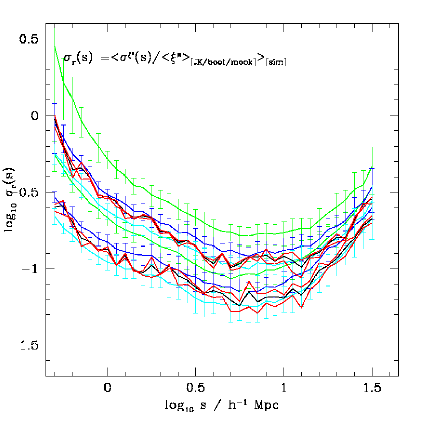
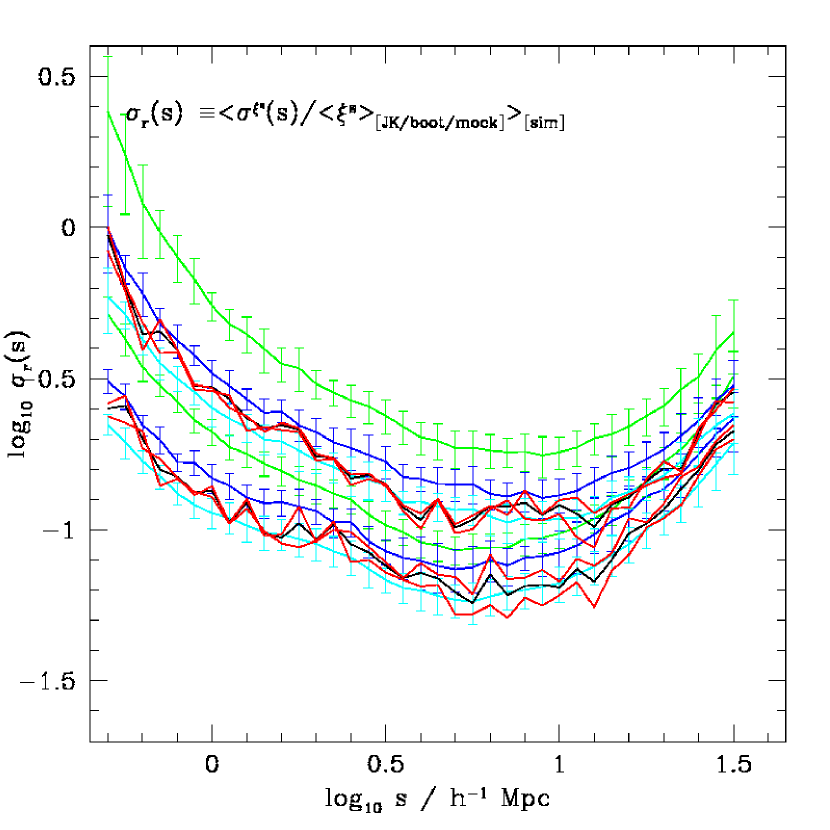
5.5 An improvement to the bootstrap recipe

Throughout our comparisons we have seen that the bootstrap gives errors that are systematically larger than the “truth” (see for example Figs. 2 and 8). Previously, we have set $N_{r}$=$N_{sub}$, i.e. the number of sub-volumes chosen with replacement was equal to the number of sub-volumes each data set is divided up into. This is an arbitrary choice and there is no reason why we cannot increase the number of sub-volumes used to define each realization of the data set. Here we consider varying the number of sub-volumes chosen. We also consider increasing the number of sub-volumes the data set is split into, which affects both the bootstrap and jackknife methods (recall that in the jackknife, the choice of $N_{sub}$ sets the number of realizations we can generate).

In the left panel of Fig. 11 we show the impact of changing the number of sub-volumes chosen on the relative variance obtained from the bootstrap with $N_{sub}$$=27$. Two families of 5 different coloured curves are shown: the top ones correspond to a sampling fraction of 10 % of the standard mean number density, while the bottom ones corresponds to a 25 % sampling fraction. Each family is composed of three bootstrap samples ($N_{r}$=1, 2, 3 $N_{sub}$, in green, blue and cyan respectively) and three mock curves: all mocks in black, and two red curves for the 50 first and 50 last respectively. The relative variance decreases as the number of sub-volumes selected increases, with the biggest change coming when the number of sub-volumes is oversampled by a factor of two (blue line). With an oversampling of a factor of 3 (cyan line), the bootstrap errors are in very good agreement with those derived from the external estimate. If we increase the oversampling rate further, the relative variance returned by the bootstrap becomes too small (not shown for clarity). From this figure, an oversampling factor of about three seems to be optimal, i.e. selecting at random, with replacement, $N_{r}$=3 $N_{sub}$ sub-volumes from the original list of length $N_{sub}$.

We note that the left panels of Figs. 2 and 11, in which the density of objects in the data set is varied, give extremely valuable information on how the relative errors scale for samples with different mean densities, as together they span an order of magnitude variation in the mean density. Increasing the mean density by a factor 2.5 leads to a reduction in the relative variance error by $\sim 80$ % (top versus bottom black lines in Fig. 11), while a mean density 4 times larger decreases the relative error by a further 50 %, at which stage the change becomes more scale dependent. Indeed, the shape of the mean relative variance in the left panel of Fig. 2 is slightly different to those in Fig. 11. We attribute this to the fact that there is a limiting number density beyond which the errors are not any longer dominated by sample shot-noise.

The right panel of Fig. 11 shows the same information as the left panel, but for a different number of sub-samples: 125 instead of 27. The remarkable point to realize here is that both panels are virtually identical, leading to the conclusion that the precise number of sub-samples the data is split into is not a primary factor for determining the size of bootstrap errors. This is in strong contrast to jackknife errors for which we observed, in Fig. 2, a systematic change in the relative variance as function of scale with respect to the mocks, with increasingly discrepant results on smaller scales for the jackknife analysis with increasing number of sub-samples.

So on adopting this essentially new prescription for the bootstrap error analysis, i.e. allowing for bootstrap resamplings of typically three times the number of sub-samples considered ($N_{r}$=3 $N_{sub}$), what is the impact on the other results presented in Sections 4 to 5? This question is best answered in Figs. 12 and 13, which show the same information as Figs. 7 and 8, but for bootstrap estimates with $N_{r}$=3 $N_{sub}$.

Fig. 12 is a great contrast to the messy Fig. 7: this time internal error estimates seem to return CI which are in much better agreement with the “truth”. We show, together with the mock CI in black, two sets of bootstrap estimates, each applied to one hundred different data sets: Boot-27 (in red) and Boot-125 (in green) with $N_{r}$=3 $N_{sub}$. We also note that the mock contour is on average $\sim 50$ % larger than in Fig. 7. This is due to the 25 % lower number density considered in this case, which is in good agreement with the findings of Fig. 11, for which we also found a typical $\sim 50$ % change in error w.r.t. the reference mean number density.

Fig. 13 present the distributions of the relative area statistic for a suite of internal error estimators, all estimated over the range 1 to $\sim 22~{}{\,h^{-1}\,{\rm Mpc}}$, with N${}_{\rm pca}=6$. In the left panel, we show the distributions of the standard bootstrap estimates with $N_{r}$=$N_{sub}$ and those of the corresponding jackknife estimates: Boot-27 in red, Boot-125 in green, Jack-27 in blue, Jack-64 in cyan and Jack-125 in magenta. In the right panel, we show the distributions for bootstrap with $N_{r}$=3 $N_{sub}$: Boot-27 in red, Boot-64 in blue and Boot-125 in green.

Fig. 13 makes several points. First it becomes clear from the right panel that the number of sub-samples drawn, with replacement, from a set of $N_{sub}$ sub-samples has to be typically three times larger than $N_{sub}$ for bootstrap errors to best reproduce the “true” mock inferred errors with minimal bias. Secondly, once that regime is reached, bootstrap errors are only very marginally dependent on the number of sub-samples the data set is split into, i.e. once the criteria on the number of data points discussed in Hartlap et al. (2007) is satisfied. For our clustering statistics, this seems to be true once $N_{sub}$ is at least 5 times larger than N_pca. Thirdly, the log-normal variance is limited to $\sigma\sim 0.15$. Hence in the absence of bias, the area of the CI are known to within a factor of 2 (with a 95 % confidence level), explicitly meaning that an estimated 2-$\sigma$ CI can be mistaken to be pessimistically a true $\sim 1.3$-$\sigma$ or optimistically a true 3-$\sigma$. Finally the observed systematic bias seen in Fig. 13 is actually less important than it looks, as the uncertainty on the mock error is larger for the number density considered here. For $f=0.25$, we observe a $\sim 20$ % scatter on the mock error, which is more than twice as large compared to our findings with $f=1.0$ (see §5.2).

Additionally, the left hand panel of Fig. 13, once compared to Fig. 8, shows that the dispersion on the internal error estimates seem to be rather insensitive to the actual number density of the samples analysed. Decreasing the sampling rate down to 25 % of the original (as in Fig. 13) makes barely any difference to the quoted dispersions, as long as the distributions of relative areas are still well described by Gaussians. On the other hand, the bias seems to be a much stronger function of the assumed mean number density, with lower number densities tending to systematically overestimate the errors by quite a significant amount. This is explicitly shown by the large mean values of each relative area distribution shown in the left panel, ranging from $\sim 1.3$ to as large as $\sim 6.6$ in the case of Jack-125. The bias increases by 1.5 to 2.5 times, depending on the estimator, when the mean density becomes 4 times smaller. When the bias becomes so large and the changes so unpredictable, it is no longer clear whether there is any positive side to be seen with these traditional internal estimators.

Figure 12: Same as Fig. 7, but for $N_{r}$=3 $N_{sub}$. The “true” error estimate is given by the mock errors (thick black), while red (dotted) correspond to Boot-27 and green (dot-dashed) to Boot-125. This plot is a great contrast to the much messier Fig. 7. The fits are done over the projected scales indicated in the figure. See text for further comments.

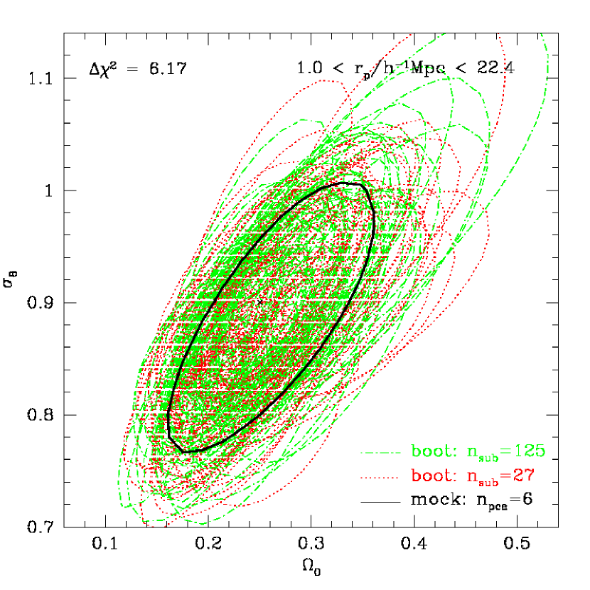
6 Summary and Conclusions

In this paper we have carried out an extensive comparison of the relative performance of internal and external error estimators for two-point clustering statistics. We devise a set of numerical experiments, extracting independent data sets from N-body simulations. The data sets are chosen to have a volume comparable to that of the typical L_⋆ volume limited samples constructed from the SDSS. The benchmark for this exercise is the error estimate obtained from the scatter over our independent data sets, which we refer to as “mock” errors or “truth”. This is then compared to internal estimates made using the jackknife and bootstrap techniques (e.g. Tukey 1958; Efron 1979). We revisit the assumptions and the free parameters behind these techniques to see if we can lay down a recipe that would reproduce the more expensive (and not even always possible) external errors. We summarize below our findings, starting with uncorrelated statistics, followed by covariance matrix based results and ending with the conclusions drawn from a case study, aimed at fitting two cosmological parameters to our clustering results.

Figure 13: The distribution of the figure of merit, similar to Fig. 8, but for $N_{r}$=$N_{sub}$ (left panel) and $N_{r}$=3 $N_{sub}$(right panel), assuming a mean number density of 25 % L_⋆ (as opposed to a L_⋆ mean number density as in Fig. 8). The figure legend gives the exact meaning of all the lines. The dotted lines are the corresponding Gaussian distributions with similar variance and mean. Increasing the number of sub-samples randomly drawn, with replacement, from the set of $N_{sub}$ sub-samples radically changes the relative area distributions.

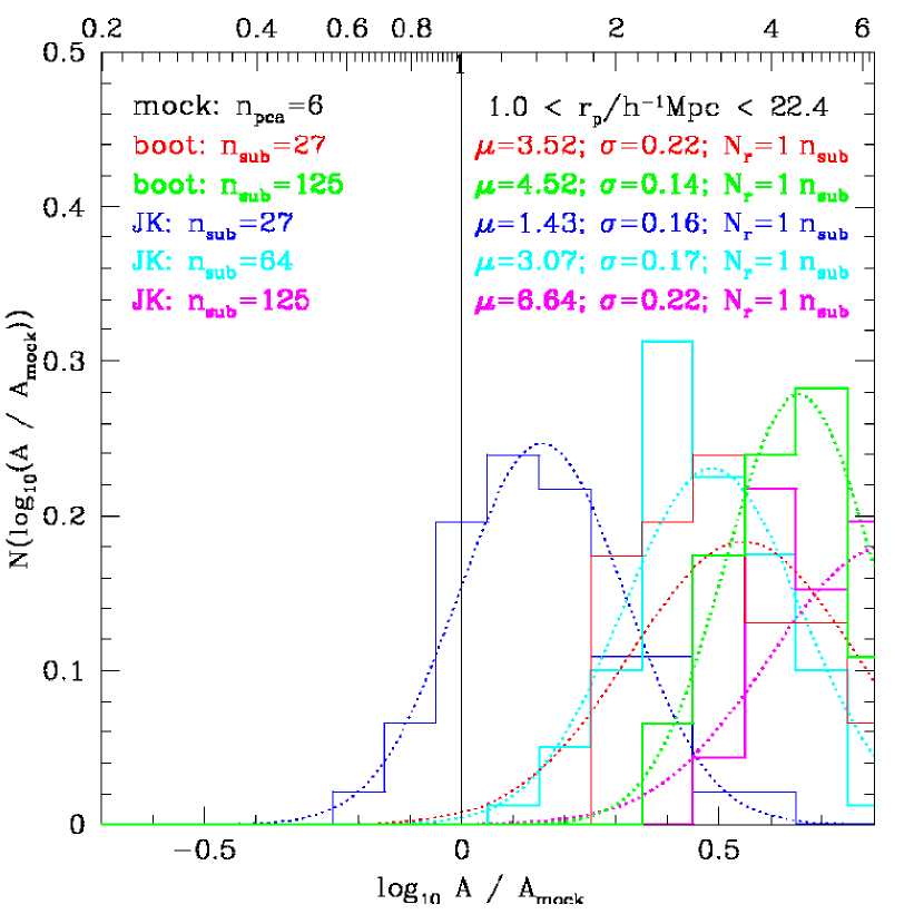
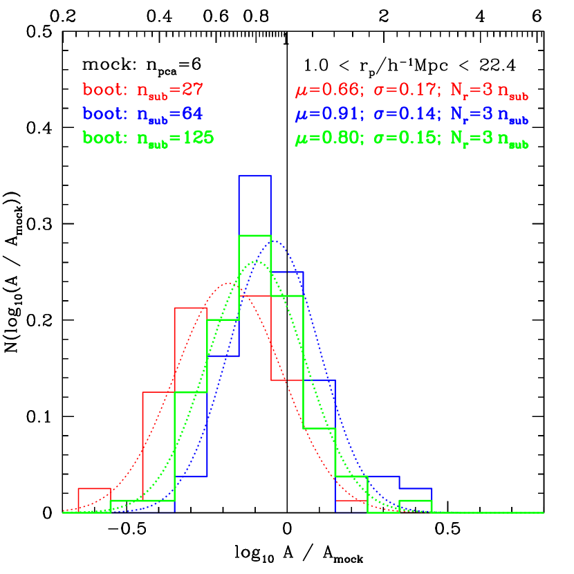
Perhaps surprisingly (as they are so widely used in the literature), we find that both internal estimators of the errors have worrying failings. Neither was able to faithfully reproduce the relative variance of the external estimate, over a limited range of scales (0.5 to 25$~{}{\,h^{-1}\,{\rm Mpc}}$). At face value, the standard bootstrap variance is nearly 50 % larger on all scales, where standard refers to the case for which the number of sub-samples selected at random, with replacement, equals the number of sub-samples the data set is divided into (i.e. $N_{r}$=$N_{sub}$). In §5.5, we solve this problem of the overestimated variance simply by increasing $N_{r}$ by a factor of three, i.e. by setting $N_{r}$=3 $N_{sub}$. The variance measured with the jackknife method is fairly accurate on large scales (greater than $10~{}{\,h^{-1}\,{\rm Mpc}}$), but the variance on small scales (less than 2-3 ${\,h^{-1}\,{\rm Mpc}}$) is clearly overestimated by a significant amount and in a method dependent way: the bias depends strongly on the number of sub-volumes the data set is split into, as explicitly shown in Fig. 2. Another major result from Section 4.3 is that all error estimators considered present Gaussianly distributed errors on the smallest projected separations. However, slowly but surely, the error distributions become non-Gaussian already on 6 (15) ${\,h^{-1}\,{\rm Mpc}}$ and larger for the jackknife (bootstrap) method, while they all remain Gaussian for the mocks over the full range of scales considered.

The details of the recovered covariance matrices, or more precisely the recovered principal component decomposition of the covariance matrices for our 100 data sets, show equally worrying features in Sections 4.4 and 4.5. Generally speaking bootstrap inferred (normalized) eigenvalues and eigenvectors are in good agreement with mock inferred ones, while jackknife inferred (normalized) eigenvalues and eigenvectors present distinctive features which are not present in the mocks and, furthermore, are also dependent on the number of sub-volumes the data set is split into. These features are particularly sensitive to the smallest scales used: as for the variance estimates, the jackknife method becomes increasingly discrepant w.r.t. the mocks when scales smaller than 2-3 ${\,h^{-1}\,{\rm Mpc}}$ are used. However, the direct influence of those subtle differences in a such technical analysis is hard to grasp and hence a better understanding in reached on an example scenario.

In Section 5 we present a case study in which the different error estimation methods are used to extract constraints on cosmological parameters from measurements of the projected correlation function, using 100 independent data sets. The discrepancy in the relative variance returned by the different methods, as described above, propagates through this analysis and gives different constraints on the fitted parameters. We quantify these differences in terms of the area of the confidence interval which would correspond to 2-$\sigma$ for the case of a two parameter fit for Gaussian distributed measurements. With 100 independent data sets, we find that the internal estimators return, on average, error ellipses with larger area than that found in the mocks, resulting indirectly into a redefinition of the confidence limit of the measurement. This is particularly true for standard bootstrap estimates, for which the number of sub-samples selected at random with replacement equals the number of sub-samples the data set is divided into (i.e. $N_{r}$=$N_{sub}$). However, we show in §5.5 that increasing the number of sub-samples drawn at random by a factor of three (i.e. $N_{r}$=3 $N_{sub}$) solves most problems: in that case, the confidence intervals are only marginally different to the mock ones. In the case of jackknife errors, the area of the error ellipse is to some extent sensitive to the number of sub-volumes the data set is split into. For all error estimators, we find, as expected, that the error ellipse area is sensitive to the number of principal components used in the analysis.

The diagnosis for the internal estimators is therefore mixed. The jackknife method has problems recovering the scale dependence of errors and the results are sensitive to the number of sub-samples the data set is split into. There is little scope to fix these problems given the definition of the method; the only thing we can vary is the number of sub-samples into which the data set is split. We did not find one choice for the number of sub-samples which could cure all of the ailments of this method. The prognosis for the bootstrap is on the other hand more encouraging. The problem of overestimating the variance can be traced to the effective volume of the data set used when the number of sub-volumes chosen at random with replacement is equal to the number of sub-volumes the data set is divided into. By oversampling the sub-volumes, this problem can be fixed, with the effective volume used tending to the original data set volume. Better still, for our application at least, there appears to be an optimal factor, three times, to oversample, with higher rates producing too little variance.

Unfortunately there seems to be no hard and fast rules for the best way to set about a principal component analysis of the covariance matrix of clustering measurements. The value of the principal component analysis is that it helps break down the information contained in a clustering measurement. The measurement will be expressed in a restricted number of bins. The choice of the number of bins is arbitrary. Using more bins does not necessarily imply that there will be more information in the correlation function. The PCA breaks the covariance matrix down into eigenvectors. These are ranked in terms of how much information or variance they contain. The variance drops quickly with the order of the eigenvector for the examples we considered, indicating that most of the information in the clustering measurements can be broken down into a few terms. The best advice we can give here would be to compare the results obtained using different numbers of eigenvectors and choose a value where the results and conclusions do not change significantly.

The analysis presented in this paper is applicable to any galaxy or cluster survey with three dimensional information. Some of the issues discussed relating to redshift space distortions are particular to local surveys in which the distant observer approximation does not hold. A new set of experiments would be required to extend our results to the calculation of errors for photometric surveys, which look at angular clustering, or to multi-band photometric surveys, which will use photometric redshifts to look at clustering in redshift slices. The projection involved in these catalogues changes the underlying statistics, making them look more Gaussian perhaps. This is the most likely explanation why Cabré et al. (2007) find such a good agreement between jackknife and mock errors for angular clustering statistics.

References

- [XX XX] Angulo R.E., Baugh C.M., Frenk C.S., Lacey C.G., 2008, MNRAS, 383, 755
- [XX XX] Barrow J.D., Bhavsar S.P., Sonoda D.H., 1984, MNRAS, 210 19
- [XX XX] Baugh C.M., 2008, Phil. Trans. A., in press
- [XX XX] Berlind A.A., et al., 2003, ApJ, 593, 1
- [XX XX] Bothun G.D., Geller M.J., Beers T.C., Huchra J.P., 1983, ApJ 268, 47
- [XX XX] Cabré A., et al., 2007, MNRAS 381, 1347
- [XX XX] Cabré A. & Gaztañaga E., 2008, arXiv:0807.2460
- [Colless et al. 2001] Colless M., et al., 2001, MNRAS, 328, 1039
- [Croton et al. 2004] Croton D.J., et al., 2004, MNRAS 352, 1232
- [Croton et al. 2007] Croton D.J., et al., 2007, MNRAS 379, 1562
- [XX XX] Efron B., 1979, Annals of Statistics, 7, 1
- [XX XX] Efron B., Tibshirani R.J., 1993, An Introduction to the Bootstrap, Chapman & Hall
- [XX XX] Efstathiou G. & Moody S.J., 2001, MNRAS 325, 1603
- [XX XX] Eisenstein D. & Hu W., 1998, ApJ 496, 605
- [XX XX] Fisher K.B., Davis M., Strauss M.A., Yahil A., Huchra J., 1994, MNRAS, 266, 50
- [Gaztañaga 1994] Gaztañaga E., 1994, MNRAS, 268, 913
- [Gaztañaga 2005] Gaztañaga E., Norberg P., Baugh C.M., Croton D.J., 2005, MNRAS 364, 620
- [XX XX] Hamilton A.J.S., 1993a, ApJ, 406, 47
- [XX XX] Hamilton A.J.S., 1993b, ApJ, 417, 19
- [XX XX] Hartlap J., Simon P., Schneider P., 2007, A&A 464, 399
- [XX XX] Hawkins E., et al. 2003, MNRAS 346, 78
- [XX XX] Kaiser N., 1987, MNRAS, 227, 1
- [XX XX] Kendall M., 1975, Multivariate Analysis, Charles Griffin & Company, London
- [XX XX] Landy S.D. & Szalay A.S., 1993, ApJ, 412, 64
- [XX XX] Lewis A. & Challinor A., 2002, PhRvD 66b, 3531
- [XX XX] Li C., et al., 2006, MNRAS 368, 21
- [XX XX] Li C., et al., 2007, MNRAS 376, 984
- [XX XX] Ling E.N., Frenk C.S., Barrow J.D., 1986, MNRAS, 223, 21
- [XX XX] Lucey J.R., 1979, PhD Thesis
- [XX XX] Maddox S.J., Esftathiou G., Sutherland W.J., Loveday J., 1990, MNRAS, 242, 43
- [XX XX] Madgwick D.S., et al., 2003, MNRAS, 344, 847
- [XX XX] Matsubara T., 2000, ApJ 535, 1
- [XX XX] Miller R.G., 1974, Biometrika, 61, 1
- [XX XX] Mo H.J., Jing Y.P., Börner G., 1992, ApJ 392, 452
- [XX XX] Norberg P., et al., 2001, MNRAS 328, 64
- [XX XX] Norberg P., et al., 2002, MNRAS 332, 827
- [XX XX] Norberg P., et al., in preparation [SAGS-V and/or SAGS-VI]
- [XX XX] Norberg P. & Porciani C., in preparation
- [XX XX] Padmanabhan N., White M., Eisenstein D., 2007, MNRAS 376, 1702
- [XX XX] Peacock J.A. & Dodds S.J., 1994, MNRAS, 267, 1020
- [XX XX] Percival W., et al., 2001, MNRAS 327, 1297
- [XX XX] Percival W., et al., 2007, MNRAS 381, 1053
- [XX XX] Press W.H., Teukolsky S.A., Vetterling W.T., Flannery B.P., 1992, Numerical Recipes in C, Cambridge University Press.
- [XX XX] Porciani C., Norberg P., 2006, MNRAS 371, 1824
- [XX XX] Quenouille G., 1956, Biometrika 43, 353
- [XX XX] Sanchez A.G., et al., 2006, MNRAS 366, 189
- [XX XX] Sanchez A.G., Baugh C.M., Angulo R., 2008, MNRAS submitted (arXiv0804.0233)
- [XX XX] Scranton R., et al., 2002, ApJ 579, 48
- [XX XX] Shao J., 1986, Annals of Statistics, 14, 1322.
- [XX XX] Szapudi I., 2004, ApJ 614, 51
- [XX XX] Tegmark M., et al., 2006, PhRvD 74, 123507
- [XX XX] Tukey J.W., 1958, Ann. Math. Stat. 29, 614
- [York et al. 2000] York, D.G. et al, AJ, 120, 1579, 2000
- [XX XX] Zehavi I., et al., 2002, ApJ 571, 172
- [XX XX] Zehavi I., et al., 2004, ApJ, 608, 16
- [XX XX] Zehavi I., et al., 2005, ApJ 630, 1