Automated lag-selection for multi-step univariate time series forecast using Bayesian Optimization: Forecast station-wise monthly rainfall of nine divisional cities of Bangladesh

Rainfall is an essential hydrological component, and most of the economic activities of an agrarian country like Bangladesh depend on rainfall. An accurate rainfall forecast can help make necessary decisions and reduce the damages caused by heavy or low to no rainfall. The monthly average rainfall is a time series data, and recently, long short-term memory (LSTM) neural networks are being used heavily for time series forecasting problems. One major challenge of forecasting using LSTMs is to select the appropriate number of lag values. In this research, we considered the number of lag values selected as a hyperparameter of LSTM; it, with the other hyperparameters determining LSTMs structure, has been optimized using Bayesian optimization. We used our proposed method to forecast rainfall for nine different weather stations of Bangladesh. Finally, the performance of the proposed model has been compared with some other LSTM with different lag-selection methods and some several popular machine learning and statistical forecasting models.

Keywords: Phase II trial; two-stage design; optimal design; single-arm trial; sample size.

1 Introduction

Bangladesh has a largely agrarian economy; its agriculture comprises about 18.6 percent of its GDP and employs around $45$ percent of the total labor force [1]. Rainfall is one central element of the hydrological process, and a significant portion of the agricultural production system depends on rainfall water through irrigation. Because of this dependency, a significant deviation in rainfall can cause severe damage to the economy. The damage is two-fold. At one extreme, if the rainfall is inadequate or highly irregular, it can cause drought [2]. Bangladesh faces a significant drought every 2.5 years [3], which is the major drawback to ensuring the food security of Bangladesh despite significant improvement in food production because drought affects the agricultural sector in Bangladesh during the production of rice, which is the major crop of Bangladesh [4]. At another extreme, because of excessive rainfall, floods can occur because Bangladesh geographically has a unique setting for flooding. About 80 percent of the landmass of Bangladesh is plain, while most parts of the country are low-lying, and as a result, it is highly vulnerable to the threat of repeated floods. From $1971-2014$, on average, 6.31 million people become victims of floods yearly, and the total monetary value of the damage was $12232.70$ million USD [5]. Another problem becoming a primary concern in Bangladesh, especially in the urban areas, is water logging caused by heavy rainfall. A recent study shows that 76 percent of traffic movement gets disrupted, 82 percent of the roads get damaged, and 68 percent of the water gets polluted in the waterlogged areas [6].

As the losses are because of the events caused by deviations in rainfall, it is necessary to forecast rainfall accurately. Additionally, accurate rainfall can help policymakers to make essential decisions regarding different agricultural policies, especially for a country like Bangladesh. However, there has not been much research on forecasting rainfall more accurately. Among the available research, studies by Mahmud et al. [7], and Mahsin et al. [8] are notable.

In contrast to Bangladesh, different time series forecasting methods have been used for forecasting rainfall in the literature. Many statistical, machine learning (ML), and neural network (NN) based models have been proposed in the literature to forecast rainfall in different parts of the world. Among the statistical methods, seasonal autoregressive integrated moving average (SARIMA) is the most commonly used [9, 10] because of its capability of producing both point and interval forecasts and the well-defined Box-Jenkins method for selecting the best model [11]. ML models like support vector regression (SVR) and random forest (RF) have also been implemented successfully for rainfall forecasting [12]. Among the NN models for forecasting rainfall, the use of single hidden-layer artificial NN models [13, 14], convolutional neural network (CNN) models are noticeable [15]. Recurrent neural network (RNN)[16] models can capture the temporal relationship between different inputs and, as a result, are being used for time-series forecasting problems [17, 18]. However, RNN faces vanishing gradient problem [19] and, as a result, fails to capture the long-term time dependence in time series. In this regard, long short-term memory (LSTM) neural networks [20] are particularly helpful for time series forecasting. Recently, LSTM has been extensively used for forecasting rainfall [21] as well as many other time series problems like demand forecasting [22], wind power forecasting, and many more [23]. In much experimental research, LSTM has been shown to perform better than other neural network structures for time series forecasting [24, 22].

One of the major challenges of using a NN-based model is to find the best set of hyperparameters because the performance of a neural network model is highly dependent on its hyperparameters. The number of hyperparameters in a NN model is higher than in other ML models like SVM or RF. The most commonly used method is searching for hyperparameters manually. Nevertheless, it becomes inconvenient when the number of hyperparameters is enormous, as it is pretty easy for someone to misinterpret the trends of the hyperparameters [25]. As a result, using automatic search algorithms is necessary. Grid search, an automatic search algorithm that trains a ML model with each combination of possible values of hyperparameters on the training set and outputs hyperparameters that produce the best possible result, was proposed [26]. However, as the number of hyperparameters increases, so does the number of combinations. Thus, grid search becomes inconvenient for computationally costly functions like LSTM models, which contain many hyperparameters. Random search, another automatic search algorithm that searches random combinations of hyperparameters within a range of values, is more feasible computationally but unreliable for training complex models [27]. In this regard, Bayesian optimization (BO) combines prior information about the unknown function with sample information to obtain posterior information on the function distribution using the Bayes formula. Based on this posterior information, BO decides where the function obtains the optimal value. In many experiments, BO has been found to outperform other global optimization algorithms [28]. Recently, BO has been extensively used for finding the best set of hyperparameters while using NN models for sequential data [29].

The inputs for forecasting time series models using ML or NN-based models are simply past observations. The selection of the number of past observations or LAGS significantly affects the forecasts. Selecting LAGS too small might be inadequate to learn the pattern of the time series data; on the other hand, selecting LAGS more than needed can make the model unnecessarily complex and overfit the model and hence produce bad forecasts. The most common approach for selecting LAGS is to consider it as a hyperparameter and search manually [22]. The problem with this approach is that if the number of hyperparameters considered is large, considering LAGS as another hyperparameter, multiply the possible number of combinations several times. Another common manual approach to select this is to analyze the partial autocorrelation function (PACF) values and stop when the plot starts diminishing [30]. One problem with this approach is that the PACF generally explains the linear correlation between the values and cannot capture non-linear trends in the series, while most machine learning and deep learning-based models are not linear. Another approach is to fix a particular set of hyperparameters, monitor the loss function, and search for LAGS, after which the loss function gets flattened. The limitation of this approach is that there is no guarantee that an optimal value of lags for one set of hyperparameters is optimal for another set of hyperparameters. Among the automated methods, selecting LAGS equal to the seasonal length is standard. Another approach is to select it equal to the length of the forecasting horizon. Moreover, Hewamalage et al. used a heuristic approach to multiply the forecast horizon or seasonal period by 1.25 and use this value in the selected LAGS [31].

Note that none of these automated methods consider LAGS as a hyperparameter. In this research, we considered LAGS as a hyperparameter in addition to the hyperparameters associated with the structure of the LSTM; thus, we automated the process of selecting Lag values using BO. Then we applied our proposed method to forecast total rainfall data for nine divisional cities of Bangladesh: Barisal, Dhaka, Comilla, Mymensingh, Rangpur, Chittagong, Rajshahi, Sylhet, and Khulna. To compare the performance of our proposed model, two popular machine learning models, RF and SVR, and two popular statistical time series forecasting techniques, SARIMA and exponential smoothing (ETS), are used.

2 Methodology

2.1 Overview of Recurrent neural network and Long Short-Term Memory network

The recurrent neural network (RNN) is a bioinspired neural network model [16] that uses the output of any stage as an input of the next step and thus captures the temporal relationship between inputs and, as a result, is widely used for modeling where a temporal relationship is present such as time series forecasting problems. For comparing RNN with other Neural Network structures, for producing the output of a particular state, the RNN considers information from the previous state in addition to the information from the inputs. In general, the weights of the RNN model are optimized using back-propagation through time (BTT) [32]. The major limitation of the RNN model is that it suffers from the vanishing gradient problem and, as a result, faces information loss in case of long-term dependence [19].

The Long short-term memory (LSTM) network is a particular type of RNN [20] which can learn long-term dependence. The main difference between the LSTM and traditional RNN is that instead of using the input units and previous state units to update the state vector, it computes the output by implementing three gate units: forget gate unit, the input gate unit, and the output gate unit. These gate units control the flow of information from the input and current state to the next state. Similar to RNN, the associated weights of LSTMs are also optimized using BTT. Some major hyperparameters associated with LSTM are the number of hidden layers, number of hidden units in the layers, learning rate, dropout rate, batch size, etc.

2.2 Overview of Gaussian Bayesian Optimization

Suppose $f(x)$ is a computationally expensive function lacking a known structure and does not have observable first or second-order derivatives, and as a result, finding solutions using Newton or quasi-Newton is not possible. Bayesian Optimization (BO) is a class of optimization algorithms focusing on solving the following problem.

$$max_{x\epsilon A}f(x).$$

BO has two main components: an objective function ($f(x)$) and a Bayesian Statistical model, $p(x,f(x))$. The second component $p(x,f(x))$ is used for modeling the objective function, which describes potential values for $f(x)$ at a candidate point $x$ and an acquisition function for deciding where to sample next.

A Gaussian regression process is typically selected as the statistical model, which considers the prior distribution to be multivariate normal (MVN) with a particular mean vector and covariance matrix. At first, some initial steps are used to build the prior MVN density. Suppose, the set $k$ pairs of parameters and their corresponding objective function values after $k$ initial steps $D=$ $(x_{1},f(x_{1}))$, $(x_{2},f(x_{2}))$,$\ldots$,$(x_{k},f(x_{k}))$. The mean vector of the prior MVN distribution is constructed by evaluating a mean function $\mu_{0}$ at each $x_{i}$. The covariance matrix, $\Sigma_{0}$, is constructed by evaluating a specific covariance function or kernel at each pair of points $(x_{i},x_{j})$. The kernel is chosen so that the points that are closer in the input space are more positively correlated, which means if $||x-x^{\prime}||<||x-x^{\prime\prime}||$, then $\Sigma_{0}(x,x^{\prime})>\Sigma_{0}(x,x^{\prime\prime})$ where $||.||$ is some distance function. The usual choices for the kernel are the Gaussian or Matern kernel.

Expected improvement is used as the acquisition function [25]. After $n^{th}$ evaluation, the expected improvement at point $x$ can be written as

$$EI_{n}(x)=E_{n}\big{[}(f(x)-f_{n}^{*})^{+}\big{]}$$

where, $f_{n}^{*}=max[f(x_{1}),f(x_{2}),...,f(x_{n})]$ and $a^{+}=max(0,a)$. And the posterior density is updated as

$$f(x)|f(x_{1:n})\sim MVN(\mu_{n}(x),\Sigma_{n}(x))$$

where, $\mu_{n}(x)=\mu_{0}(x)+\Sigma_{0}(x,x_{1:n})\Sigma_{0}(x_{1:n},x_{1:n})^{-1}\big{(}f(x_{1:n})-\mu_{0}(x_{1:n})\big{)}$ and $\Sigma_{n}(x)=\Sigma_{0}(x,x)-\Sigma_{0}(x,x_{1:n})\Sigma_{0}(x_{1:n},x_{1:n})^{-1}\Sigma_{0}(x_{1:n},x)$. The next evaluation is done on the point where $EI_{n}(x)$ is maximum. The outline of BO for maximum number of iteration $N$ is described below

• Initialize the prior $p(x,f(x))$.

• For every iteration $i\leq N$,

  • Obtain the new set of hyperparameter by solving

    $$\hat{x}=argmax_{x}EI_{n}(x).$$

  • Evaluate the objective function at $\hat{x}$ as $f(\hat{x})$.

  • Update $p(x,f(x))$ by finding the posterior distribution using $D=D\cup\big{(}\hat{x},f(\hat{x})\big{)}$.

• Stop if $i=N$ or any other stopping criteria has been fulfilled.

2.3 Data Splitting and forecasting strategy

For every station, we split the data set into three parts: training, validation, and test data set. The training data set is used for training a specific model, and the validation data set is used to monitor the performance of the trained model and find the best candidate model. One common approach while splitting the data set in this manner is to equal the length of the validation and test data set [33, 34]. Suppose $\mathbf{y}=(y_{1}$, $y_{2}$, $y_{3}$, …, $y_{T})$ be the time series data with $T$ observations, where $y_{t}$ indicates the observed data at $t^{th}$ timepoint. If $|Tr|$, $|V|$, and $|Te|$ be the length of training, validation, and test series, respectively, we can write the three series as follows.

• Training: $\mathbf{y}_{Tr}=(y_{1},...,y_{T-(|V|+|Te|)})$

• Validation: $\mathbf{y}_{V}=(y_{T-(|V|+|Te|-1)},...,y_{T-|Te|})$

• Test: $\mathbf{y}_{Te}=(y_{T-|Te|+1},...,y_{T})$

Note that, $\mathbf{y}_{Tr}$, $\mathbf{y}_{V}$ and $\mathbf{y}_{Te}$ contains the first $|Tr|$, the next $|V|$ and the last $|Te|$ observations of $\mathbf{y_{T}}$. Also, $|Tr|+|V|+|Te|=T$ and $|V|=|Te|$. Then we normalize $\mathbf{y}_{Tr}$, $\mathbf{y}_{V}$ using

$$\mathbf{z}_{Tr}=\frac{\mathbf{y}_{Tr}-\min(\mathbf{y}_{Tr})}{\max(\mathbf{y}_{Tr})-\min(\mathbf{y}_{Tr})},\text{ and}$$ (1)

$$\mathbf{z}_{V}=\frac{\mathbf{y}_{V}-\min(\mathbf{y}_{Tr})}{\max(\mathbf{y}_{Tr})-\min(\mathbf{y}_{Tr})}.$$ (2)

For univariate time series forecasting problems, the inputs at a time point are simply the previous observations of that series. Suppose the number of lag values considered as input is $m$, then the input matrix $\mathbf{X}(m)$ and output vector $\mathbf{y}(m)$ can be expressed as

$$\mathbf{X}(m)=\begin{bmatrix}z_{1}&z_{2}&z_{3}&\ldots&z_{m}\\ z_{2}&z_{3}&z_{4}&\ldots&z_{m+1}\\ \vdots&\vdots&\vdots&\ldots&\vdots\\ z_{Tr-m}&z_{Tr-m}&z_{Tr-m+1}&\ldots&z_{Tr-1}\end{bmatrix},\text{ and}$$ (3)

$$\mathbf{y}(m)=(z_{m+1},z_{m+1},\ldots,z_{Tr}).$$ (4)

After training the model using $\mathbf{z}_{Tr}$, suppose we want to forecast for the next $|V|$ time points, say $\mathbf{\hat{z}}_{V}=\big{(}\hat{z}_{T-(|V|+|Te|-1)}$, $\hat{z}_{T-(|V|+|Te|-2)}$, $...$, $\hat{z}_{T-|Te|)}\big{)}$. In our study, a multi-step forecasting scheme [35] is considered. The input vector for forecasting at time point $|Tr|+h$ using a model that selected LAG as $m$, $\mathbf{x_{|Tr|+h}}$ can be expressed as the following.

$$\mathbf{x}_{|Tr|+h}=\begin{cases}(z_{Tr},\ldots,z_{|Tr|+m-1}),&\text{if $h=1$}\\ (\hat{z}_{|Tr|+h-1},\ldots,\hat{z}_{|Tr|+1},y_{|Tr|},...,z_{|Tr|+m+h-2})&\text{if $1<h<=m$}\\ (\hat{z}_{|Tr|+h-1},\ldots,\hat{z}_{|Tr|+1},z_{|Tr|})&\text{if $m>h$}\\ \end{cases}$$ (5)

Here the input for the first forecast contains information from observed values, but the second and later forecast values will be dependent on both the observed values and previously forecasted values.

2.4 Use Bayesian Optimization to find the optimal lag

The dimension of $\mathbf{X}(m)$ is $(Tr-m)\times m$ and the length of $\mathbf{y}(m)$ is $Tr-m$. Note that the values and dimensions of $\mathbf{X}(m)$ and $\mathbf{y}(m)$ depend on $m$. That is why $\mathbf{X}(m)$ and $\mathbf{y}(m)$ can be written as a function of $m$. We will use this relationship to find the optimal value of $m$ using Bayesian Optimization. Let $H_{1}$ be the set of hyperparameters associated with the structure of LSTM models. Our study also considers the number of selected lags as a hyperparameter. Then the set of hyperparameters we want to find the optimal value of any loss function is $H=(m,H1)$.

In general, the search space of BO is continuous. On the other hand, $m$ is discrete. Additionally, some other hyperparameters can be discrete. To mitigate this problem, instead of $H$, we use BO to optimize another set of hyperparameters $H2$ where every element of $H2$ takes continuous values. Before training an LSTM model, we convert $H2$ into $H$ by using

$$H=g(H2).$$ (6)

Here the function $g(.)$ operates element-wise and rounds the evelemt only if it is discrete; else keeps the original value. Finally, we consider the negative of mean squared error as the objective function, which can be expressed as

$$f(H2)=\displaystyle-\frac{\sum_{i=T-(|V|+|Te|-1)}^{T-|Te|}(z_{i}-\hat{z}_{i})^{2}}{|V|}.$$ (7)

The negative sign is taken in 7 because, by default, BO finds the maximum possible value, but any forecasting algorithm’s objective is to get as less $RMSE$ as possible.

In a single iteration of BO, we do the following.

1. Convert $H2$ into $H$ using $H=(m,H1)=g(H2)$.

2. Find $\mathbf{X}(m)$ and $\mathbf{y}(m)$ is found from the training data set using equation 3 and 4.

3. Train a model using structural hyperparameter set $H1$.

4. Use the trained model has been used to find forecasts for the next $|V|$ timepoints,

5. After that, the value of the objective function $f(H)$ has been found for this particular set of hyperparameter ($H$).

2.5 Train the final proposed model

The model with the highest $f(H)$ value in the BO process only uses information from $\textbf{y}_{Tr}$. If we use this model as our finalized model, our final forecast may disregard the change in pattern that might occur in the last part ($\textbf{y}_{V}$. As a result, it is necessary to train the final model using information from training and validation data [36].

Suppose the optimized set of hyperparameters from BO is $H_{Opt}=(m_{Opt},H1_{Opt})$. For training the final model, we first normalize the training and validation data set ($\mathbf{y}_{Tr,V}$) to get $\mathbf{y}_{Tr,V}$. Then use $\mathbf{z}_{Tr,V}$ to get $\mathbf{X}(m_{Opt})$ and $\mathbf{y}(m_{Opt})$ via the data splitting process mentioned in subsection 2.3. Finally, train a model using the hyperparameter set $H1_{Opt}$. After that, this finalized model forecasts for the next $|Te|$ time points. Suppose the forecasts using this model is $\hat{\mathbf{z}}_{Te}$. Finally, we get the final forecast by denormalizing $\hat{\mathbf{z}}_{Te}$ using

$$\hat{\mathbf{y}}_{Te}=\hat{\mathbf{z}}_{Te}\times\big{(}\max(\mathbf{y}_{Tr,V})-\min(\mathbf{y}_{Tr,V})\big{)}+\min(\mathbf{y}_{Tr,V})$$ (8)

The entire process of finding optimal $m$ and training our proposed model is given in Figure 1.

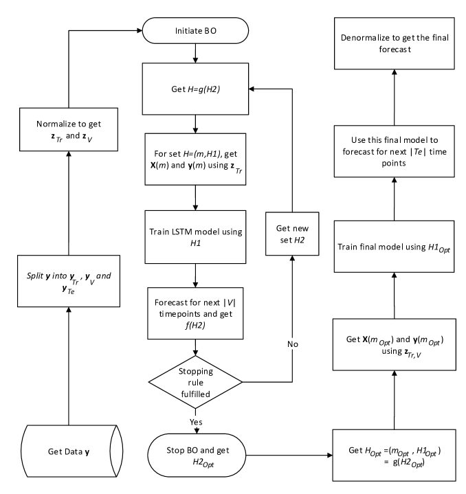
Figure 1: Overview of the whole process

2.6 Evaluation criteria for point forecast

To evaluate the performance of point forecasts, we use four measures. According to all these four measures, a lower value implies that a model performs better than a model having a higher value. Suppose $y_{1},y_{2},y_{3},\ldots,y_{h}$ be the observed values and if $\hat{y}_{1},\hat{y}_{2},\hat{y}_{3},\ldots,\hat{y}_{H}$ are the point forecasts on the same time points.

Then the first two measures, root mean squared error ($RMSE$) and mean absolute error ($MAE$), can be expressed as

$$RMSE=\displaystyle\sqrt{\frac{\sum_{i=1}^{h}(y_{i}-\hat{y}_{i})^{2}}{h}},$$ (9)

and

$$MAE=\displaystyle\frac{\sum_{i=1}^{h}(|y_{i}-\hat{y}_{i}|)}{h}.$$ (10)

Here $h$ is the length of the forecasting horizon. Additionally, to evaluate the performance of the forecasts relative to the actual values, we use symmetric mean absolute percentage error ($SMAPE$) that can be defined as:

$$SMAPE=\displaystyle\frac{100\%}{h}\sqrt{\sum_{i=1}^{h}\frac{|y_{i}-\hat{y}_{i}|}{(|y_{i}|+|\hat{y_{i}}|)/2}}$$ (11)

However, $SMAPE$ is unstable with values close to zero [37]. In this regard, Suilin [36] proposed to replace the denominator of 11 by the following:

$$max(|y_{i}|+|\hat{y_{i}}|+\epsilon,0.5+\epsilon)$$ (12)

This alternate measure skips dividing by values close to zero by replacing those with an alternative positive constant. We set the hyperparameter $\epsilon=0.1$, suggested by Suilin [36].

Finally, we use average rank ($ARank$). If $\hat{y}_{i,m}$ be the forecast for timepoint $i$ by model $m$, then $ARank$ can be defined as

$$ARank=\sum_{i=1}^{h}\frac{R_{i,m}}{h},$$ (13)

where $R_{i,m}$ is the rank of forecast of time point $i$ by model $m$ among the $M$ candidate model in ascending order. The lowest and highest possible value of $ARank$ is $1$ and $M$, respectively.

2.7 Comparing the performance of multiple methods

According to any standard measure, if the performance of a model is found to be better than all other candidate models, then it is easy to conclude that the method is better. However, if no model is found superior in every case, then it is necessary to conduct statistical tests to compare their performances [38]. The two-step testing procedure proposed by Demsar [39] can be used in this regard. This method was primarily developed to compare classification methods over multiple data sets. Later, Abbasimehra et al. [40] implemented this method for comparing multiple forecasting models over multiple data sets. For this, according to that particular measure, rank has been found for different models and datasets, and the average rank for each method is calculated. Then for the first testing step, a hypothesis test is performed to check whether there is any significant difference in the performance of any two proposed models. If the result is significant, pairwise post hoc tests have been performed.

Suppose we have applied $k$ algorithms on $N$ total data sets, and according to any measure, $r_{i}^{j}$ is the rank of the $j^{th}$ algorithms on the $i^{th}$ data set. For the first step, a Friedman statistic has been compute using

$$\chi_{F}^{2}=\displaystyle\frac{12N}{k(k+1)}\Big{[}\sum_{j}R_{j}^{2}-\displaystyle\frac{k(k+1)^{2}}{4}\Big{]},$$

where $R_{j}=\sum_{i=1}^{N}r_{i}^{j}$ is the average rank of $j^{th}$ algorithm. Under the null hypothesis ($H_{0}$) that all the models perform identical $\chi_{F}^{2}$ follows a $\chi^{2}$ distribution with $(k-1)$ degrees of freedom ($df$). However, Iman and Davenport [41] showed that Friedman’s $\chi_{F}^{2}$ is undesirably conservative and proposed a different test statistic that can be stated as

$$F_{F}=\displaystyle\frac{(N-1)\chi_{F}^{2}}{N(k-1)-\chi_{F}^{2}}$$ (14)

which follows as a $F-$distribution with $df$ $(k-1)$ and $(k-1)(N-1)$ under $H_{0}$. If $H_{0}$ is rejected in the first step, only then the second-stage testing is performed, where Hochberg’s post hoc test is used to check whether the reference model performs better than the other candidate models using the statistic

$$z_{Model}=\displaystyle\frac{R_{Model}-R_{Reference}}{\sqrt{\displaystyle\frac{k(k+1)}{6N}}}.$$ (15)

Here the reference model is our proposed model. The critical values of $z_{Model}$ can be found in a standard normal distribution table. For Hochberg’s test, the p-values of the $z$ values for $(k-1)$ comparisons with the control model are first computed and sorted from the smallest to the largest. Finally, the $i^{th}$ model is called significantly different from the reference model if the $p-value$ is smaller than $\frac{i}{k}\alpha$.

3 Case study

3.1 Selected models for comparison

For comparing the performance of the proposed model ($PROP$) for different data sets we consider the following models.

1. LSTM with number of past observations= seasonal length ($LSL$).

2. LSTM with number of past observations= forecasting horizon ($LFH1$).

3. LSTM with number of past observations= seasonal length $\times 1.25$ ($LFH1p25$).

4. Support vector regression ($SVR$).

5. Random Forest ($RF$).

6. Seasonal autoregressive moving average ($SARIMA$).

7. Exponential smoothing ($ETS$).

For the model $1-3$, similar strategy as $PROP$ has been considered except the number of lag values has been before training the models and other hypperparameters has been optimized using BO. Additionally, because $RF$ and $SVR$ are not too computationally extensive, we use grid search to find the best set of hyperparameters for them [42, 43]. In this case, the similar data-splitting process mentioned in subsection 2.3 is used.

3.2 Libraries used

To implement our proposed method, we used Python library TensorFlow to train LSTM models and bayesopt for implementing BO. Additionally, to fit the two machine learning models: RF and SVR models, Python libraries sklearn has been used. On the other hand, to fit the two statistical forecasting models: SARIMA and ETS, the package forecast programming language R has been used.

3.3 Data and preprocessing

The data sets are taken from Bangladesh Meteorological Department. Out of the 35 weather stations, in this research, rainfall data of nine selected stations those are located in the nine divisional districts named as: Barisal (BR), Chittagong (CH), Comilla (CM), Dhaka (DH), Khulna (KH), Mymensingh (MY), Rajshahi (RJ), Rangpur (RN) and Sylhet (SY). The starting and ending months are given in table 1. The data sets contain no missing values. Then every data set is split into 3 parts: training, validation and test. For every cases, we keep the length of the validation and test series fixed as $60$ which means $|V|=|Te|=60$.

Table 1: Starting and ending months and the number of missing values for the Rainfall data of 9 stations

	BR	CH	CM	DH	KH	MY	RJ	RN	SY
Start	1948-01	1949-01	1948-01	1953-01	1948-01	1948-01	1964-01	1954-01	1956-01
End	2020-07	2020-10	2020-08	2020-10	2020-08	2020-08	2020-09	2020-07	2020-07

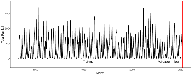
Figure 2: Data splitting process for station DH

To check the stationarity of our series, we first perform an augmented Dicky-Fuller (ADF) test [44]. Since none of the $p-values$ are bigger than $0.05$, we reject the null hypothesis stating that the data is non stationary for every series. Then because neural network models cannot model seasonality perfectly [45], we first deseasonalize the series using STL decomposition and then proceed with the deseasonalized series for training using $PROP$ modeld. Note that, the process of testing nonstationarity and deseasonalizing the data is performed only on the training and validation data sets; we keep the test data sets intake because we do not want the performance on the actual data sets, not on the transformed ones.

Table 2: Statistic value from ADF test

	BR	CH	CM	DH	KH	MY	RJ	RN	SY
$Statistic$	-12.479	-16.696	-11.139	-10.787	-13.043	-11.662	-16.073	-11.729	-11.922
$p-value$	$0.010$	$0.010$	$0.010$	$0.010$	$0.010$	$0.010$	$0.010$	$0.010$	$0.010$

3.4 Results

In our experiment, apart from the number of lag values as input ($m$), we are considering five LSTM hyperparameters: dropout rate ($dr$), learning rate($lr$), number of hidden units in hidden layer 1 ($hu_{1}$), number of hidden units in layer 2 ($hu_{2}$) and batch size ($b$).Hence the set of hyperparameters ($H_{1}$) we want to optimize using BO has six items. The selected lag values for $PROP$ are given in Table 3.

Table 3: Selected Lags using for $PROP$

BR	CH	CM	DH	KH	MY	RJ	RN	SY
34	32	36	45	34	38	31	33	35

Figure 3: Observed and forecasted monthly rainfall by all candidate methods for all stations.

The performance of $PROP$ and the other selected models are given in Table 4. Among the four LSTM considered, $PROP$ performs better than the other three LSTM models since it has the lowest $RMSE$, $MAE$, $SMAPE$, and $ARank$ values among them for all stations. On the other hand, $LSL$ constantly performs worse than the other three LSTM models, regardless of what measure we use for evaluating the performance. This provides evidence that the selected lag for for $LSL$, $12$ is insufficient for training an LSTM. The comparison between $LFH1$ and $LFH1p25$ is not consistent. $LFH1p25$ has lower $RMSE$ and $MAE$ for station RN; and has lower $SMAPE$ for station CH. For all other stations, $LFH1$ performs better than $LFH1p25$.

Table 4: Performance of forecasts from all candidate models.

Measure	Model	Station
		BR	CH	CM	DH	KH	MY	RJ	RN	SY
RMSE	LSTM	18.270	12.679	14.677	11.999	13.966	12.952	15.497	15.884	14.696
	LSL	21.792	15.467	17.598	14.234	16.193	16.655	18.002	18.148	18.035
	LFH1	18.720	12.929	14.788	12.024	14.058	13.165	15.895	16.257	14.810
	LFH1p25	18.858	13.164	14.977	12.474	14.354	13.254	16.045	16.197	14.969
	SVR	19.142	12.061	16.030	15.595	15.194	14.170	18.977	16.498	14.805
	RF	17.662	12.583	19.173	16.852	16.818	13.195	17.233	16.004	14.972
	SARIMA	21.972	20.163	16.869	17.848	19.688	15.402	17.768	22.214	15.992
	ETS	25.721	16.555	15.123	16.474	20.379	13.575	18.228	17.452	14.833
MAE	LSTM	12.884	7.528	11.161	9.176	9.610	6.983	11.346	9.923	9.739
	LSL	15.519	9.116	13.179	10.934	11.448	8.491	13.296	11.594	11.880
	LFH1	13.133	7.654	11.223	9.248	9.666	7.042	11.584	10.115	9.836
	LFH1p25	13.210	7.765	11.422	9.429	9.893	7.234	11.662	10.111	9.949
	SVR	13.006	7.924	12.171	10.544	10.324	7.757	13.278	10.471	9.675
	RF	11.911	8.243	14.802	11.503	11.875	7.489	12.608	10.077	9.823
	SARIMA	14.232	11.455	12.183	12.351	12.578	8.932	13.906	12.668	10.093
	ETS	22.774	11.403	11.862	12.761	17.159	7.552	14.309	11.567	10.938
SMAPE	LSTM	14.765	8.950	13.203	11.227	12.870	9.563	12.917	11.420	10.489
	LSL	18.025	10.923	15.489	13.704	15.454	11.864	15.426	13.363	13.108
	LFH1	15.118	9.021	13.268	11.291	12.982	9.642	13.227	11.601	10.605
	LFH1p25	15.145	9.198	13.549	11.497	13.239	9.956	13.238	11.611	10.756
	SVR	14.253	9.880	14.629	12.132	13.120	10.746	14.201	12.284	9.867
	RF	13.348	10.032	17.173	13.302	15.279	10.322	14.093	11.688	10.049
	SARIMA	15.143	11.678	14.680	14.390	15.366	12.780	17.004	14.341	10.530
	ETS	26.688	13.838	14.519	14.946	21.855	10.513	16.277	13.677	11.567
ARank	LSTM	3.683	3.300	3.950	3.717	3.367	3.383	3.450	3.317	3.933
	LSL	6.000	5.550	5.967	6.183	5.833	5.883	5.900	5.717	6.383
	LFH1	4.150	3.667	4.033	4.167	3.617	3.617	4.083	3.883	4.117
	LFH1p25	3.950	4.100	4.483	4.183	4.067	4.050	4.333	4.117	4.467
	SVR	3.833	4.483	4.200	3.817	4.100	4.950	4.417	4.717	4.150
	RF	3.733	4.567	4.450	4.300	4.750	4.333	4.267	3.917	4.150
	SARIMA	4.200	4.550	4.233	4.467	4.183	5.183	4.817	4.733	3.983
	ETS	6.450	5.783	4.683	5.167	6.083	4.600	4.733	5.600	4.817

Additionally, we can easily conclude that $PROP$ performs better than $SARIMA$ and $ETS$ since it has lower $RMSE$, $MAE$, $MAE$ and $ARank$ values for all stations. In case if we consider $ARank$ as our metric, $PROP$ performs better than the other for all stations. However, the comparison between $RF$ and $SVR$ is more complex. $RF$ has the lowest $RMSE$ and $MAE$ for one station each. On the other hand, $SVR$ has the lowest $RMSE$, $MAE$, and $SMAPE$ for one, one, and two stations, respectively. As a result, to check whether $PROP$ performs better than these two models, using the two-step procedure mentioned in the subsection 2.7 is necessary.

To complete Desmar’s two-step test, we first rank the models based on the $RMSE$ in ascending orders for every station and then calculate the average rank for every station; and finally, use these average ranks for performing the procedure mentioned in section 2.7. From Table 5, the $(F_{F},p-value)$ pairs for testing whether there is any difference in the performance of the models are $(13.430,0.000)$, $(21.518,0.000)$ and $(15.341,0.000)$ for $RMSE$, $MAE$ and $SMAPE$ respectively. Since all the corresponding $p-values$ are very small, we conclude that the performance of at least two models is not identical, and we proceed to the second stage of Desmar’s two-step test.

Table 5: Two-step testing for comparing the performances of $PROP$ with other candidate models.

Measure		Step 1	Step 2
		$F_{F}$	$z_{LSL}$	$z_{LFH1}$	$z_{LFH1p25}$	$z_{SVR}$	$z_{RF}$	$z_{SARIMA}$	$z_{ETS}$
$RMSE$	$Statistic$	13.430	4.330	1.155	2.021	2.791	2.598	4.907	4.138
	$p-value$	0.000	0.000	0.248	0.043	0.005	0.009	0.000	0.000
$MAE$	$Statistic$	21.518	4.523	1.251	1.925	2.502	2.694	5.004	4.811
	$p-value$	0.000	0.000	0.211	0.054	0.012	0.007	0.000	0.000
$SMPE$	$Statistic$	15.341	4.426	0.866	1.925	2.021	2.309	4.234	4.619
	$p-value$	0.000	0.000	0.386	0.054	0.043	0.021	0.000	0.000

In the second step, we consider $10\%$ significance level. In Table 5, we see that all $z-values$ are positive for every model across all measures, which is analogous to the fact that $PROP$ has a lower average rank according to $RMSE$, $MAE$, and $SMAPE$.

Here we have seven models for comparison. We say $PROP$ performs better than the model with $i^{th}$ smallest $p-value$ if it is smaller that $0.10\frac{i}{7}$. We conclude that we can conclude that $PROP$ performs better than all models except $LFH1$. It should be noted that, according to all the measures $PROP$ performs better that $LFH1$ yet we cannot reject the null hypothesis here. This happens because $LFH1$ perform better than the other candidate models except $PROP$, and as a result, it has average ranks smaller than others. Additionally, the performance of the other models can be ranked using the $p-values$ in the second step from table 5. The models with higher $p-values$ indicate that the model is performing close to $PROP$ as they are tougher to reject, and it can be said that they are performing better than the models having smaller $p-values$. For example, according to $RMSE$, $LFH1$ performs better than $LFH1p25$. In general, according to all three measures, $LFH1$ performs better than all other models, and $ETS$ performs the worst. Additionally, the two machine learning models $RF$ and $SVR$ perform better than the two statistical methods ($ETS$ and $SARIMA$), but they got outperformed by $LFH1$ and $LFH1p25$. We have not completed the two-step test for $ARank$ since $PROP$ has lower values than all other candidate models across all stations.

4 Conclusion

In this study, we used BO to find the optimal lag inputs of $LSTM$ for forecasting monthly average rainfall of nine weather stations of Bangladesh. Then we compared models developed by our proposed model with some other models and showed that our model outperforms those methods in most of the cases.

Among the limitations of the study, the most obvious one is that rainfall is not solely dependent on past observations; rather, it depends on many factors like air quality, latitude, elevation, topography, seasons, distance from the sea, and coastal sea-surface temperature and many other factors. Moreover, the study has been done only for the stations located in the divisional cities of Bangladesh rather than considering all the stations of Bangladesh because the data for other stations were not available.

The second major drawback is that we used a Gaussian Bayesian Optimization for finding the optimal set of hyperpaprameters of $LSTM$ that naturally searches for continuous hyperparametes. LAGS and some other hyperparameters are discrete on the other hand. As a result, during training our proposed model, we lost some information because of using the conditional rounding function.

For potential future extensions, a study that uses other variables like temperature, location information, air quality can improve forecasting accuracy. Recently, parzen tree based Bayesian optimization algorithms has been popular as they have the capability to consider discrete space for hyperparameters. So we can suspect that using Parzen Tree based algorithms might further improve the proposed method.

References

- Kamruzzaman and Shaw [2018] Md. Kamruzzaman and Rajib Shaw. Flood and sustainable agriculture in the haor basin of bangladesh: A review paper. Universal Journal of Agricultural Research, 6:40–49, 2018. doi: https://doi.org/10.1007/s00500-016-2474-6.
- Shafie et al. [2009] H Shafie, S R Halder, A K M M Rashid, K S Lisa, and H A Mita. Endowed wisdom: knowledge of nature and coping with disasters in bangladesh. Dhaka: Center for Disaster Preparedness and Management., 2009.
- Murad1 and Islam [2011] Hasan Murad1 and A K M Saiful Islam. Drought assessment using remote sensing and gis in north-western region of bangladesh. International Conference on Water & Flood Management, pages 797–804, 2011.
- Kashem and Faroque [2013] M. Kashem and M. Faroque. A country scenarios of food security and governance in bangladesh. Journal of Science Foundation, 9:41–50, 2013. doi: 10.3329/jsf.v9i1-2.14646.
- Kabir and Hossen [2019] Md. Humayain Kabir and Md. Nazmul Hossen. Impacts of flood and its possible solution in bangladesh. Disaster Advances, 22:387–408, 2019. doi: https://doi.org/10.1007/s00500-016-2474-6.
- Alam et al. [2023] Rafiul Alam, Zahidul Quayyum, Simon Moulds, Marzuka Ahmad Radia, Hasna Hena Sara, Md Tanvir Hasan, and Adrian Butler. Dhaka city water logging hazards: area identification and vulnerability assessment through GIS-remote sensing techniques. Environmental Monitoring and Assessment, 195(5):543, May 2023. ISSN 0167-6369, 1573-2959. doi: 10.1007/s10661-023-11106-y.
- Mahmud et al. [2016] Ishtiak Mahmud, Sheikh Hefzul Bari, and M. Tauhid Ur Rahman. Monthly rainfall forecast of bangladesh using autoregressive integrated moving average method. Environmental Engineering Research, 22(2):162–68, 2016. doi: https://doi:10.4491/eer.2016.075.
- Mahsin et al. [2012] Md Mahsin, Yasmin Akhter, and Maksuda Begum. Modeling rainfall in dhaka division of bangladesh using time series analysis. Journal of Mathematical Modelling and App, 1:67–73, 2012.
- Narayanan et al. [2013] Priya Narayanan, Ashoke Basistha, Sumana Sarkar, and Sachdeva Kamna. Trend analysis and arima modelling of pre-monsoon rainfall data for western india. Comptes Rendus Geoscience, 345(1):22–27, 2013. ISSN 1631-0713. doi: https://doi.org/10.1016/j.crte.2012.12.001.
- Eni and Adeyeye [2015] Daniel Eni and Fola J. Adeyeye. Seasonal arima modeling and forecasting of rainfall in warri town, nigeria. Journal of Geoscience and Environment Protection, 3(06), 2015.
- Bartholomew [1971] D. J. Bartholomew. Time series analysis forecasting and control. Operational Research Quarterly (1970-1977), 22(2):199–201, 1971. ISSN 00303623.
- Yu et al. [2017] Pao-Shan Yu, Tao-Chang Yang, Szu-Yin Chen, Chen-Min Kuo, and Hung-Wei Tseng. Comparison of random forests and support vector machine for real-time radar-derived rainfall forecasting. Journal of Hydrology, 552:92–104, 2017. ISSN 0022-1694. doi: https://doi.org/10.1016/j.jhydrol.2017.06.020.
- Mishra et al. [2018] Neelam Mishra, Hemant Kumar Soni, Sanjiv Sharma, and A K Upadhyay. Development and analysis of artificial neural network models for rainfall prediction by using time-series data. Intelligent Systems and Applications, 1:16–23, 2018.
- Lee et al. [2018] Jeongwoo Lee, Chul-Gyum Kim, Jeong Eun Lee, Nam WonKim, and Hyeonjun Kim. Application of artificial neural networks to rainfall forecasting in the geum river basin, korea. Water, 10(10), 2018. ISSN 2073-4441. doi: 10.3390/w10101448.
- Haidar and Verma [2018] Ali Haidar and Brijesh Verma. Monthly rainfall forecasting using one-dimensional deep convolutional neural network. IEEE Access, 6:69053–69063, 2018. doi: 10.1109/ACCESS.2018.2880044.
- Lipton et al. [2015] Zachary C. Lipton, John Berkowitz, and Charles Elkan. A critical review of recurrent neural networks for sequence learning, 2015.
- Cen and Wang [2019] Zhongpei Cen and Jun Wang. Crude oil price prediction model with long short term memory deep learning based on prior knowledge data transfer. Energy, 169:160–171, 2019. ISSN 0360-5442. doi: https://doi.org/10.1016/j.energy.2018.12.016.
- Yang et al. [2019] Fangfang Yang, Weihua Li, Chuan Li, and Qiang Miao. State-of-charge estimation of lithium-ion batteries based on gated recurrent neural network. Energy, 175:66–75, 2019. ISSN 0360-5442. doi: https://doi.org/10.1016/j.energy.2019.03.059.
- Bengio et al. [1994] Y. Bengio, P. Simard, and P. Frasconi. Learning long-term dependencies with gradient descent is difficult. IEEE Transactions on Neural Networks, 5(2):157–166, 1994. doi: 10.1109/72.279181.
- Hochreiter and Schmidhuber [1997] Sepp Hochreiter and Jürgen Schmidhuber. Long short-term memory. Neural Computation, 9(8):1735–1780, 1997. doi: 10.1162/neco.1997.9.8.1735.
- Kumar et al. [2019] Deepak Kumar, Anshuman Singh, Pijush Samui, and Rishi Kumar Jha. Forecasting monthly precipitation using sequential modelling. Hydrological Sciences Journal, 64(6):690–700, 2019. doi: 10.1080/02626667.2019.1595624.
- Abbasimehr et al. [2020a] Hossein Abbasimehr, Mostafa Shabani, and Mohsen Yousefi. An optimized model using lstm network for demand forecasting. Computers & Industrial Engineering, 143:106435, 2020a. ISSN 0360-8352. doi: https://doi.org/10.1016/j.cie.2020.106435.
- Xiang et al. [2020] Zhongrun Xiang, Jun Yan, and Ibrahim Demir. A rainfall-runoff model with lstm-based sequence-to-sequence learning. Water Resources Research, 56(1):25–26, 2020. doi: https://doi.org/10.1029/2019WR025326.
- Yunpeng et al. [2017] Liu Yunpeng, Hou Di, Bao Junpeng, and Qi Yong. Multi-step ahead time series forecasting for different data patterns based on lstm recurrent neural network. In 2017 14th Web Information Systems and Applications Conference (WISA), pages 305–310, 2017. doi: 10.1109/WISA.2017.25.
- Wu et al. [2019] Jia Wu, Xiu-Yun Chen, Hao Zhang, Li-Dong Xiong, Hang Lei, and Si-Hao Deng. Hyperparameter optimization for machine learning models based on bayesian optimization. Journal of Electronic Science and Technology, 17(1):26–40, 2019. ISSN 1674-862X. doi: https://doi.org/10.11989/JEST.1674-862X.80904120.
- James et al. [2013] Gareth James, Daniela Witten, Trevor Hastie, and Robert Tibshirani. An introduction to statistical learning, volume 112. Springer, 2013.
- Bergstra and Bengio [2012] James Bergstra and Yoshua Bengio. Random search for hyper-parameter optimization. Journal of Machine Learning Research, 13:281–305, 2012.
- Jones [2001] Donald R. Jones. A taxonomy of global optimization methods based on response surfaces. Journal of Global Optimization, 21:345–383, 2001. doi: 10.1023/A:1012771025575.
- Cabrera et al. [2020] Diego Cabrera, Adriana Guamán, Shaohui Zhang, Mariela Cerrada, René-Vinicio Sánchez, Juan Cevallos, Jianyu Long, and Chuan Li. Bayesian approach and time series dimensionality reduction to lstm-based model-building for fault diagnosis of a reciprocating compressor. Neurocomputing, 380:51–66, 2020. ISSN 0925-2312. doi: https://doi.org/10.1016/j.neucom.2019.11.006.
- Yuan et al. [2019] Xiaohui Yuan, Chen Chen, Min Jiang, and Yanbin Yuan. Prediction interval of wind power using parameter optimized beta distribution based lstm model. Applied Soft Computing, 82:105550, 2019. ISSN 1568-4946. doi: https://doi.org/10.1016/j.asoc.2019.105550.
- Hewamalage et al. [2021a] Hansika Hewamalage, Christoph Bergmeir, and Kasun Bandara. Recurrent neural networks for time series forecasting: Current status and future directions. International Journal of Forecasting, 37(1):388–427, 2021a. ISSN 0169-2070. doi: https://doi.org/10.1016/j.ijforecast.2020.06.008.
- Werbos [1990] P.J. Werbos. Backpropagation through time: what it does and how to do it. Proceedings of the IEEE, 78(10):1550–1560, 1990. doi: 10.1109/5.58337.
- Hewamalage et al. [2021b] Hansika Hewamalage, Christoph Bergmeir, and Kasun Bandara. Recurrent neural networks for time series forecasting: Current status and future directions. International Journal of Forecasting, 37(1):388–427, 2021b. ISSN 0169-2070. doi: https://doi.org/10.1016/j.ijforecast.2020.06.008.
- Bandara et al. [2020] Kasun Bandara, Christoph Bergmeir, and Slawek Smyl. Forecasting across time series databases using recurrent neural networks on groups of similar series: A clustering approach. Expert Systems with Applications, 140:112896, 2020. ISSN 0957-4174. doi: https://doi.org/10.1016/j.eswa.2019.112896.
- Ben Taieb et al. [2012] Souhaib Ben Taieb, Gianluca Bontempi, Amir F. Atiya, and Antti Sorjamaa. A review and comparison of strategies for multi-step ahead time series forecasting based on the nn5 forecasting competition. Expert Systems with Applications, 39(8):7067–7083, 2012. ISSN 0957-4174. doi: https://doi.org/10.1016/j.eswa.2012.01.039.
- Suilin and Abdulaziz [2017] Arthur Suilin and Mohamed Abdulaziz. Kaggle-web-traffic. https://https://github.com/Arturus/kaggle-web-traffic, 2017.
- Hyndman et al. [2008] Rob Hyndman, Anne B Koehler, J Keith Ord, and Ralph D Snyder. Forecasting with exponential smoothing: the state space approach. Springer Science & Business Media, 2008.
- Protopapadakis et al. [2019] Eftychios Protopapadakis, Dimitrios Niklis, Michalis Doumpos, Anastasios Doulamis, and Constantin Zopounidis. Sample selection algorithms for credit risk modelling through data mining techniques. International Journal of Data Mining, Modelling and Management, 11(2):103–128, 2019. doi: 10.1504/IJDMMM.2019.098969.
- Demsar [2006] Janez Demsar. Statistical comparisons of classifiers over multiple data sets. Journal of Machine Learning Research, 07:1–30, 2006.
- Abbasimehr et al. [2020b] Hossein Abbasimehr, Mostafa Shabani, and Mohsen Yousefi. An optimized model using lstm network for demand forecasting. Computers ‘I&’ Industrial Engineering, 143:106435, 2020b. ISSN 0360-8352. doi: https://doi.org/10.1016/j.cie.2020.106435.
- Iman and Davenport [1980] Ronald L. Iman and James M. Davenport. Approximations of the critical region of the friedman statistic. Communications in Statistics - Theory and Methods, 9(6):571–595, 1980. doi: 10.1080/03610928008827904.
- Probst et al. [2019] Philipp Probst, Marvin N. Wright, and Anne-Laure Boulesteix. Hyperparameters and tuning strategies for random forest. WIREs Data Mining and Knowledge Discovery, 9(3):e1301, 2019. doi: https://doi.org/10.1002/widm.1301.
- Bao and Liu [2006] Yukun Bao and Zhitao Liu. A fast grid search method in support vector regression forecasting time series. In Emilio Corchado, Hujun Yin, Vicente Botti, and Colin Fyfe, editors, Intelligent Data Engineering and Automated Learning – IDEAL 2006, pages 504–511. Springer Berlin Heidelberg, 2006. ISBN 978-3-540-45487-8.
- Dickey and Fuller [1979] D. Dickey and Wayne Fuller. Distribution of the estimators for autoregressive time series with a unit root. JASA. Journal of the American Statistical Association, 74, 06 1979. doi: 10.2307/2286348.
- Claveria et al. [2017] Oscar Claveria, Enric Monte, and Salvador Torra. Data pre-processing for neural network-based forecasting: does it really matter? Technological and Economic Development of Economy, 23(5):709–725, 2017. doi: 10.3846/20294913.2015.1070772.