On free boundary problems shaped by
oscillatory singularities

Abstract.

We start the investigation of free boundary variational models featuring oscillatory singularities. The theory varies widely depending upon the nature of the singular power $\gamma(x)$ and how it oscillates. Under a mild continuity assumption on $\gamma(x)$, we prove the optimal regularity of minimizers. Such estimates vary point-by-point, leading to a continuum of free boundary geometries. We also conduct an extensive analysis of the free boundary shaped by the singularities. Utilizing a new monotonicity formula, we show that if the singular power $\gamma(x)$ varies in a $W^{1,n^{+}}$ fashion, then the free boundary is locally a $C^{1,\delta}$ surface, up to a negligible singular set of Hausdorff co-dimension at least $2$.

1. Introduction

We develop a variational framework for the analysis of free boundary problems that include a continuum of singularities. The mathematical setup leads to the minimization of an energy-functional of the type

$$\mathscr{E}(v,\mathcal{O})=\int_{\mathcal{O}}{F}(Dv,v,x)\,dx,$$ (1.1)

whose Lagrangian, $F(\vec{p},v,x)$, is non-differentiable with respect to the $v$ argument, and the degree of singularity varies with respect to the spatial variable $x$. The singularity oscillation exerts an intricate influence on the free boundary’s trace and shape in a notably unpredictable manner. This dynamic not only alters the geometric behaviour of the solution but also significantly impacts the regularity of the free boundary. As a consequence, the associated Euler-Lagrange equation gives rise to a rich new class of singular elliptic partial differential equations, which, in their own right, present an array of intriguing and independent mathematical challenges and interests.

Singular elliptic PDEs, particularly those involving free boundaries, find applications in a variety of fields, including thin film flows, image segmentation, shape optimization, and biological invasion models in ecology, to cite just a few. Mathematically, such models lead to the analysis of an elliptic PDE of the form

$$\Delta u=\mathfrak{s}(x,u)\chi_{\{u>0\}},$$ (1.2)

within a domain $\Omega\subset\mathbb{R}^{n}$. The defining characteristic of the PDE above lies in the singular term $\mathfrak{s}\colon\Omega\times(0,\infty)\to\mathbb{R}$, which becomes arbitrarily large near the zero level set of the solution, i.e.,

$$\lim\limits_{v\to 0}\mathfrak{s}(x,v)=\infty.$$ (1.3)

Fine regularity properties of solutions to (1.2), along with geometric measure estimates and eventually the differentiability of their free boundaries, $\partial\{u>0\}$, are inherently intertwined with quantitative information concerning the blow-up rate outlined in (1.3). Heuristically, solutions of PDEs with a faster singular blow-up rate will exhibit reduced regularity along their free boundaries. Existing methods for treating these singular PDE models, in various forms, rely to some extent on the uniformity of the blow-up rate prescribed in (1.3).

In this paper, we investigate a broader class of variational free boundary problems, extending our focus to encompass oscillatory blow-up rates. That is, we are interested in PDE models involving singular terms with fluctuating asymptotic behavior,

$$\Delta u\sim u^{-p(x)},$$ (1.4)

for some function $p\colon\Omega\to[0,1)$. As anticipated, the analysis will be variational, i.e., we will investigate local minimizers of a given non-differentiable functional, as described in (1.1), which exhibit a spectrum of oscillatory exponents of non-differentiability.

The investigation of the static case, i.e., of PDE models in the form of $\Delta u\sim u^{-p_{0}}$, where $0<p_{0}<1$, has a rich historical lineage, tracing its roots to the classical Alt-Phillips problem, as documented in [3, 16, 17]. This elegant problem has served as a source of inspiration, sparking significant advancements in the domain of free boundary problems, as exemplified by works like [5, 8, 11, 10, 18, 19, 20, 21], to cite just a few. Remarkably, the Alt-Phillips model serves as a bridge connecting the classical obstacle problem, which pertains to the case $p_{0}=0$, and the cavitation problem, achieved as the limit when $p_{0}\nearrow 1$. Each intermediary model exhibits its own unique geometry. That is, solutions present a precise geometric behavior at a free boundary point, viz. $u\sim\text{dist}^{\beta}(x,\partial\{u>0\})$, for a critical, well-defined and uniform exponent $\beta(p_{0})$.

Mathematically, the oscillation of the singular exponent brings several new challenges, as the model prescribes multiple free boundary geometries. The main difficulty in analyzing free boundary problems with oscillatory singularities relies on quantifying how the local free boundary geometry fluctuations affect the regularity of the solution $u$ as well as the behavior of its associated free boundary $\partial\{u>0\}$. In essence, the main quest in this paper is to understand how changes in the free boundary geometry directly influence its local behaviour.

From the applied viewpoint, the model studied in this paper accounts for the heterogeneity of external factors influencing the reaction rates within the porous catalyst region where the gas density $u(x)$ is distributed. To be more specific, when examining the theory of diffusion and reaction within catalysts modeled in an isotropic, homogeneous medium, the task at hand involves the minimization of an energy-functional, which takes the form

$$\mathscr{J}(v,\mathcal{O})=\int_{\mathcal{O}}\frac{1}{2}|Dv|^{2}dx+\int_{\mathcal{O}}f(x,v)dx.$$ (1.5)

Minimizers of $\mathscr{J}$ describe the density distribution of the gas in a stationary situation. The term $\int_{\mathcal{O}}f(x,v)dx$ corresponds to the rupture law along the free boundary. It models the complexities of the catalytic reaction, dictated by the abrupt shifts and discontinuities in the reaction rates as they intersect the catalyst’s surface. Mathematically, such factors prompt the non-differentiability of the term $f(x,v)$ with respect to the $v-$argument.

The singularity of $\partial_{v}f(x,v)$ along $v=0$ carries critical information about the model’s behavior. It is a no-static feature of the model, dynamically shifting in response to several external factors, including temperature, pressure, and the roughness of the catalyst’s surface. Such considerations require mathematical models allowing for non-differentiable terms whose singularity may vary with respect to the spatial variable $x$.

In this inaugural paper, our focus is directed toward fine regularity properties of local minimizers of the energy-functional

$$J_{\delta(x)}^{\gamma(x)}(v):=\int\frac{1}{2}\left|Dv\right|^{2}+\delta(x)(v^{+})^{\gamma(x)}dx,$$ (1.6)

where the functions $\gamma(x)$ and $\delta(x)$ possess specific properties that will be elaborated upon in due course. In connection with the theory of singular elliptic PDEs, minimizers of (1.6) are distributional solutions of

$$\left\{\begin{array}[]{rllcl}\Delta u&=&\delta(x)\gamma(x)u^{\gamma(x)-1}&\mathrm{in}&\,\{u>0\}\\ Du&=&0&\mathrm{on}&\partial\{u>0\},\end{array}\right.$$

with the free boundary condition being observed by local regularity estimates, to be shown in this paper.

The paper is organized as follows. In Section 2, we discuss the mathematical setup of the problem and the scaling feature of the energy-functional (2.3). We also establish the existence of minimizers as well as local $C^{1,\alpha_{\star}}$-regularity, for some $0<\alpha_{\star}<1$, independent of the modulus of continuity of $\gamma(x)$. The final preliminary result in Section 2 concerns non-degeneracy estimates. In Section 3, we obtain gradient estimates near the free boundary, quantifying the magnitude of $Du(y)$ in terms of the pointwise value $u(y)$. We highlight that the results established in Sections 2 and 3 are all independent of the continuity of $\gamma(x)$. However, when $\gamma(x)$ varies randomly, regularity estimates of $u$ and its non-degeneracy properties along the free boundary have different homogeneities, and thus no further regularity properties of the free boundary are expected to hold. We tackle this issue in Section 4, where under a very weak condition on the modulus of continuity of $\gamma(x)$, we establish sharp pointwise growth estimates of $u$. The estimates from Section 4 imply that near a free boundary point $x_{0}\in\partial\{u>0\}$, the minimizer $u$ behaves precisely as $\sim d^{\frac{2}{2-\gamma(x_{0})}}$, with universal estimates. Section 5 is devoted to Hausdorff estimates of the free boundary. In Section 6, we obtain a Weiss-type monotonicity formula which yields blow-up classification, and in Section 7, we discuss the regularity of the free boundary $\partial\{u>0\}$.

We conclude this introduction by emphasizing that the complexities inherent in the dynamic singularities model extend far beyond the boundaries of the specific problem under consideration in this study. The challenges posed by the program put forward in this paper call for the development of new methods and tools. We are optimistic that the solutions crafted in this research can have a broader impact, proving invaluable in the analysis of a wide range of mathematical problems where similar intricacies and complexities manifest themselves.

2. Preliminary results

2.1. Mathematical setup

We start by describing precisely the mathematical setup of our problem. We assume $\Omega\subset\mathbb{R}^{n}$ is a bounded domain and $\delta,\gamma:\Omega\to\mathbb{R}_{0}^{+}$ are bounded mensurable functions.

For each subset $\mathcal{O}\subset\Omega$, we denote

$$\gamma_{\star}(\mathcal{O}):=\mathop{\operatorname*{ess\,}\inf}_{y\in\mathcal{O}}\,\gamma(y)\ \quad\mbox{and}\quad\,\gamma^{\star}(\mathcal{O}):=\mathop{\operatorname*{ess\,}\sup}_{y\in\mathcal{O}}\,\gamma(y).$$ (2.1)

In the case of balls, we adopt the simplified notation

$$\gamma_{\star}(x,r)\coloneqq\gamma_{\star}(B_{r}(x))\qquad\mbox{and}\qquad\gamma^{\star}(x,r)\coloneqq\gamma^{\star}(B_{r}(x)).$$

Throughout the whole paper, we shall assume

$$0<\gamma_{\star}(\Omega)\leq\gamma^{\star}(\Omega)\leq 1.$$ (2.2)

For a non-negative boundary datum $0\leq\varphi\in H^{1}(\Omega)\cap L^{\infty}(\Omega)$, we consider the problem of minimizing the functional

$$\mathcal{J}^{\delta}_{\gamma}(v,\Omega):=\int_{\Omega}\frac{1}{2}\left|Dv\right|^{2}+\delta(x)(v^{+})^{\gamma(x)}dx$$ (2.3)

among competing functions

$$v\in{\mathcal{A}}:=\left\{v\in H^{1}(\Omega)\ :\ v-\varphi\in H_{0}^{1}(\Omega)\right\}.$$

We say $u\in\mathcal{A}$ is a minimizer of (2.3) if

$$\mathcal{J}^{\delta}_{\gamma}(u,\Omega)\leq\mathcal{J}^{\delta}_{\gamma}(v,\Omega),\quad\forall v\in\mathcal{A}.$$

Note that minimizers as above are, in particular, local minimizers in the sense that, for any open subset $\Omega^{\prime}\subset\Omega$,

$$\mathcal{J}^{\delta}_{\gamma}(u,\Omega^{\prime})\leq\mathcal{J}^{\delta}_{\gamma}(v,\Omega^{\prime}),\quad\forall v\in H^{1}(\Omega^{\prime})\ :\ v-u\in H_{0}^{1}(\Omega^{\prime}).$$

2.2. Scaling

Some of the arguments used recurrently in this paper rely on a scaling feature of the functional (2.3) that we detail in the sequel for future reference. Let $x_{0}\in\Omega$ and consider two parameters $A,B\in(0,1]$. If $u\in H^{1}(\Omega)$ is a minimizer of $\mathcal{J}_{\gamma}^{\delta}(v,B_{A}(x_{0}))$, then

$$w(x):=\frac{u(x_{0}+Ax)}{B},\quad x\in B_{1}$$ (2.4)

is a minimizer of the functional

$${\mathcal{J}}^{\tilde{\delta}}_{\tilde{\gamma}}(v,B_{1}):=\int_{B_{1}}\frac{1}{2}\left|Dv\right|^{2}+\tilde{\delta}(x)v^{\tilde{\gamma}(x)}dx,$$

with

$$\tilde{\delta}(x):=B^{\gamma(x_{0}+Ax)}\left(\frac{A}{B}\right)^{2}\delta(x_{0}+Ax)\quad\mathrm{and}\quad\tilde{\gamma}(x):=\gamma(x_{0}+Ax).$$

Indeed, by changing variables,

$$\int_{B_{A}(x_{0})}\frac{1}{2}\left|Du(x)\right|^{2}+\delta(x)u(x)^{\gamma(x)}dx$$

$$= A^{n}\int_{B_{1}}\frac{1}{2}\left|Du(x_{0}+Ax)\right|^{2}dx+A^{n}\int_{B_{1}}\delta(x_{0}+Ax)u(x_{0}+Ay)^{\gamma(x_{0}+Ax)}dy$$

$$= A^{n}\int_{B_{1}}\frac{1}{2}\left|\left(\frac{B}{A}\right)Dw(x)\right|^{2}+\delta(x_{0}+Ax)\left[Bw(x)\right]^{\gamma(x_{0}+Ax)}dx$$

$$= A^{n-2}B^{2}\int_{B_{1}}\frac{1}{2}\left|Dw(x)\right|^{2}+B^{\gamma(x_{0}+Ax)-2}A^{2}\delta(x_{0}+Ax)\left[w(x)\right]^{\gamma(x_{0}+Ax)}dx$$

$$= A^{n-2}B^{2}\int_{B_{1}}\frac{1}{2}\left|Dw(x)\right|^{2}+\tilde{\delta}(x)\left[w(x)\right]^{\tilde{\gamma}(x)}dx.$$

Observe that since $0<B\leq 1$, $\tilde{\delta}$ satisfies

$$\|\tilde{\delta}\|_{L^{\infty}(B_{1})}\leq B^{\gamma_{\star}(x_{0},A)-2}A^{2}\|\delta\|_{L^{\infty}(B_{A}(x_{0}))}.$$

In particular, choosing $A=r$ and $B=r^{\beta}$, with $0<r\leq 1$ and

$$\beta=\frac{2}{2-\gamma_{\star}(x_{0},A)},$$

we obtain $\|\tilde{\delta}\|_{L^{\infty}(B_{1})}\leq\|\delta\|_{L^{\infty}(B_{r}(x_{0}))}$.

2.3. Existence of minimizers

We start by proving the existence of non-negative minimizers of functional (2.3) and deriving global $L^{\infty}$-bounds.

Proposition 2.1.

Under the conditions above, namely (2.2), there exists a minimizer $u\in{\mathcal{A}}$ of the energy-functional (2.3). Furthermore, $u$ is non-negative in $\Omega$ and $\|u\|_{L^{\infty}(\Omega)}\leq\|\varphi\|_{L^{\infty}(\Omega)}$.

Proof.

Let

$$m=\inf_{v\in{\mathcal{A}}}\mathcal{J}^{\delta}_{\gamma}(v,\Omega)$$

and choose a minimizing sequence $u_{k}\in{\mathcal{A}}$ such that, as $k\to\infty$,

$$\mathcal{J}^{\delta}_{\gamma}(u_{k},\Omega)\longrightarrow m.$$

Then, for $k\gg 1$, we have

$$\left\|Du_{k}\right\|_{L^{2}(\Omega)}^{2} = 2\mathcal{J}^{\delta}_{\gamma}(u_{k},\Omega)-2\int_{\Omega}\delta(x)(u_{k}^{+})^{\gamma(x)}dx$$

$$\leq 2(m+1)+2\left\|\delta\right\|_{L^{\infty}(\Omega)}\left(|\Omega|+\left\|u_{k}\right\|_{L^{1}(\Omega)}\right)$$

$$\leq 2(m+1)+2\left\|\delta\right\|_{L^{\infty}(\Omega)}\left(|\Omega|+\sqrt{|\Omega|}\left\|u_{k}\right\|_{L^{2}(\Omega)}\right).$$

From Poincaré inequality, we also have

$$\left\|u_{k}\right\|_{L^{2}(\Omega)} \leq \left\|u_{k}-\varphi\right\|_{L^{2}(\Omega)}+\left\|\varphi\right\|_{L^{2}(\Omega)}\qquad$$

$$\leq C\left\|Du_{k}-D\varphi\right\|_{L^{2}(\Omega)}+\left\|\varphi\right\|_{L^{2}(\Omega)}\qquad$$

$$\leq C\left\|Du_{k}\right\|_{L^{2}(\Omega)}+C\left\|D\varphi\right\|_{L^{2}(\Omega)}+\left\|\varphi\right\|_{L^{2}(\Omega)},\qquad$$

and so

$$\left\|u_{k}\right\|_{L^{2}(\Omega)}\leq C^{2}(4\epsilon)^{-1}+\epsilon\left\|Du_{k}\right\|^{2}_{L^{2}(\Omega)}+C\left\|D\varphi\right\|_{L^{2}(\Omega)}+\left\|\varphi\right\|_{L^{2}(\Omega)},$$ (2.5)

with $\epsilon>0$ to be chosen. We thus obtain

$$\left\|Du_{k}\right\|_{L^{2}(\Omega)}^{2}\leq C_{1}+2\epsilon\left\|\delta\right\|_{L^{\infty}(\Omega)}\sqrt{|\Omega|}\left\|Du_{k}\right\|_{L^{2}(\Omega)}^{2},$$

with

$$C_{1}=C_{1}\left(m,\left\|\delta\right\|_{L^{\infty}(\Omega)},|\Omega|,C,\epsilon,\left\|\varphi\right\|_{H^{1}(\Omega)}\right).$$

Choosing

$$\epsilon=\frac{1}{4\left\|\delta\right\|_{L^{\infty}(\Omega)}\sqrt{|\Omega|}},$$

we conclude

$$\left\|Du_{k}\right\|_{L^{2}(\Omega)}^{2}\leq 2C_{1}$$

and thus, using again (2.5), that $\left\{u_{k}\right\}_{k}$ is bounded in $H^{1}(\Omega)$. Consequently, for a subsequence (relabelled for convenience) and a function $u\in H^{1}(\Omega)$, we have

$$u_{k}\longrightarrow u,$$

weakly in $H^{1}(\Omega)$, strongly in $L^{2}(\Omega)$ and pointwise for a.e. $x\in\Omega$. Using Mazur’s theorem, it is standard to conclude that $u\in{\mathcal{A}}$.

The weak lower semi-continuity of the norm gives

$$\int_{\Omega}\frac{1}{2}\left|Du\right|^{2}dx\leq\liminf_{k\to\infty}\int_{\Omega}\frac{1}{2}\left|Du_{k}\right|^{2}dx$$

and the pointwise convergence and Lebesgue’s dominated convergence give

$$\int_{\Omega}\delta(x)(u_{k}^{+})^{\gamma(x)}dx\longrightarrow\int_{\Omega}\delta(x)(u^{+})^{\gamma(x)}dx.$$

We conclude that

$$\mathcal{J}^{\delta}_{\gamma}(u,\Omega)\leq\liminf_{k\to\infty}\mathcal{J}^{\delta}_{\gamma}(u_{k},\Omega)=m$$

and so $u$ is a minimizer.

We now turn to the bounds on the minimizer. That $u$ is non-negative for a non-negative boundary datum is trivial since $(u^{+})^{+}=u^{+}$, and testing the functional against $u^{+}\in\mathcal{A}$ immediately gives the result. For the upper bound, test the functional with $v=\min\left\{u,\|\varphi\|_{L^{\infty}(\Omega)}\right\}\in{\mathcal{A}}$ to get, by the minimality of $u$,

$$0\leq\int_{\Omega}\left|D(u-v)\right|^{2}dx = \int_{\Omega\cap\{u>\|\varphi\|_{L^{\infty}(\Omega)}\}}\left|Du\right|^{2}dx$$

$$= \int_{\Omega}\left|Du\right|^{2}-\left|Dv\right|^{2}dx$$

$$\leq 2\int_{\Omega}\delta(x)\left[(v^{+})^{\gamma(x)}-(u^{+})^{\gamma(x)}\right]dx$$

$$\leq 0.$$

We conclude that $v=u$ in $\Omega$ and thus $\|u\|_{L^{\infty}(\Omega)}\leq\|\varphi\|_{L^{\infty}(\Omega)}$. ∎

Remark 2.1.

If the boundary datum $\varphi$ changes sign, the existence theorem above still applies, but the minimizer is no longer non-negative. Uniqueness may, in general, fail, even in the case of $\gamma\equiv\gamma_{0}<1$.

2.4. Local $C^{1,\alpha}-$regularity estimates

Our first main regularity result yields local $C^{1,\alpha}-$regularity estimates for minimizers of the energy-functional (2.3), under no further assumption on $\gamma(x)$ other than (2.2).

Theorem 2.1.

Let $u$ be a minimizer of the energy-functional (2.3) under assumption (2.2). For each subdomain $\Omega^{\prime}\Subset\Omega$, there exists a constant $C>0$, depending only on $n$, $\|\delta\|_{\infty}$, $\gamma_{\star}(\Omega^{\prime})$, $\mathrm{dist}\,(\Omega^{\prime},\partial\Omega)$ and $\|u\|_{\infty}$, such that

$$\|u\|_{C^{1,\alpha}(\Omega^{\prime})}\leq C,$$

for $\alpha=\dfrac{\gamma_{\star}(\Omega^{\prime})}{2-\gamma_{\star}(\Omega^{\prime})}$.

For the proof of Theorem 2.1, we will argue along the lines of [13, 14], but several adjustments are needed, and we will mainly comment on those. We start by noting that, without loss of generality, one can assume that the minimizer satisfies the bound

$$\|u\|_{L^{\infty}(\Omega)}\leq 1.$$ (2.6)

Indeed, $u$ minimizes (2.3) if, and only if, the auxiliary function

$$\overline{u}(x):=\frac{u(x)}{M},$$

minimizes the functional

$$v\mapsto\int_{\Omega}\frac{1}{2}\left|Dv\right|^{2}+\overline{\delta}(x)(v^{+})^{\gamma(x)}\,dx,$$

where

$$\overline{\delta}(x):=M^{\gamma(x)-2}\delta(x).$$

Taking $M=\max\{1,\|u\|_{L^{\infty}(\Omega)}\},$ places the new function $\overline{u}$ under condition (2.6); any regularity estimate proven for $\overline{u}$ automatically translates to $u$.

Next, we gather some useful estimates, which can be found in [14, Lemma 2.4 and Lemma 4.1, respectively]. We adjust the statements of the lemmata to fit the setup treated here. Given a ball $B_{R}(x_{0})\Subset\Omega$, we denote the harmonic replacement (or lifting) of $u$ in $B_{R}(x_{0})$ by $h$, i.e., $h$ is the solution of the boundary value problem

$$\Delta h=0\;\text{ in }\;B_{R}(x_{0})\quad\text{ and }\quad h-u\in H^{1}_{0}(B_{R}(x_{0})).$$

By the maximum principle, we have $h\geq 0$ and

$$\|h\|_{L^{\infty}(B_{R}(x_{0}))}\leq\|u\|_{L^{\infty}(B_{R}(x_{0}))}.$$ (2.7)

Lemma 2.1.

Let $\psi\in H^{1}(B_{R})$ and $h$ be the harmonic replacement of $\psi$ in $B_{R}$. There exists $c$, depending only on $n$, such that

$$c\int\limits_{B_{R}}|D\psi-Dh|^{2}\,dx\leq\int\limits_{B_{R}}|D\psi|^{2}-|Dh|^{2}\,dx.$$ (2.8)

Lemma 2.2.

Let $\psi\in H^{1}(B_{R})$ and $h$ be the harmonic replacement of $\psi$ in $B_{R}$. Given $\beta\in(0,1)$, there exists $C$, depending only on $n$ and $\beta$, such that

$$\int\limits_{B_{r}}|D\psi-(D\psi)_{r}|^{2}\,dx \leq C\left(\frac{r}{R}\right)^{n+2\beta}\int\limits_{B_{R}}|D\psi-(D\psi)_{R}|^{2}\,dx$$

$$+C\int\limits_{B_{R}}|D\psi-Dh|^{2}\,dx,$$

for each $0<r\leq R$.

We are ready to prove the local regularity result.

Proof of Theorem 2.1.

We prove the result for the case of balls $B_{R}(x_{0})\Subset\Omega$. Without loss of generality, assume $x_{0}=0$ and denote $B_{R}:=B_{R}(0)$. Since $u$ is a local minimizer, by testing (2.3) against its harmonic replacement, we obtain the inequality

$$\int\limits_{B_{R}}|Du|^{2}-|Dh|^{2}\,dx\leq 2\displaystyle\int\limits_{B_{R}}\delta(x)\left(h(x)^{\gamma(x)}-u(x)^{\gamma(x)}\right)\,dx.$$ (2.9)

Next, with the aid of [14, Lemma 2.5], one obtains

$$h(x)^{\gamma(x)}-u(x)^{\gamma(x)}\leq|u(x)-h(x)|^{\gamma(x)},$$

and, using (2.2), together with (2.6) and (2.7), we get

$$|u(x)-h(x)|^{\gamma(x)}\leq|u(x)-h(x)|^{\gamma_{\star}(0,R)},\quad\mbox{a.e. in }\;B_{R}.$$ (2.10)

This readily leads to

$$\int\limits_{B_{R}}\delta(x)\left(h(x)^{\gamma(x)}-u(x)^{\gamma(x)}\right)\,dx\leq\|\delta\|_{L^{\infty}(\Omega)}\int\limits_{B_{R}}|u(x)-h(x)|^{\gamma_{\star}(0,R)}\,dx.$$

In addition, by combining Hölder and Sobolev inequalities, we obtain

$$\int\limits_{B_{R}}|u-h|^{\gamma_{\star}(0,R)}\,dx \leq C|B_{R}|^{1-\frac{\gamma_{\star}(0,R)}{2^{*}}}\left(\,\int\limits_{B_{R}}|u-h|^{2^{*}}\,dx\,\right)^{\frac{\gamma_{\star}(0,R)}{2^{*}}}$$ (2.11)

$$\leq C|B_{R}|^{1-\frac{\gamma_{\star}(0,R)}{2^{*}}}\left(\displaystyle\int\limits_{B_{R}}|Du-Dh|^{2}\,dx\right)^{\frac{\gamma_{\star}(0,R)}{2}}$$

for $2^{*}=\dfrac{2n}{n-2}$.

Therefore, using Lemma 2.1, together with (2.9), (2.10) and (2.11), we get

$$\int\limits_{B_{R}}|Du-Dh|^{2}\,dx\leq C|B_{R}|^{\frac{2(2^{*}-\gamma_{\star}(0,R))}{2^{*}(2-\gamma_{\star}(0,R))}}=CR^{n+2\frac{\gamma_{\star}(0,R)}{2-\gamma_{\star}(0,R)}}.$$ (2.12)

Finally, by taking

$$\beta=\frac{\gamma_{\star}(0,R)}{2-\gamma_{\star}(0,R)}\in(0,1),$$

in Lemma 2.2, we conclude

$$\int\limits_{B_{r}}|Du-(Du)_{r}|^{2}\,dx$$

$$\leq C\left(\frac{r}{R}\right)^{n+2\frac{\gamma_{\star}(0,R)}{2-\gamma_{\star}(0,R)}}\int\limits_{B_{R}}|Du-(Du)_{R}|^{2}\,dx+CR^{n+2\frac{\gamma_{\star}(0,R)}{2-\gamma_{\star}(0,R)}},$$

for each $0<r\leq R$. Campanato’s embedding theorem completes the proof. ∎

Hereafter, in this paper, we assume $\Omega=B_{1}\subset\mathbb{R}^{n}$ and, according to what was argued around (2.6), fix a normalized, non-negative minimizer, $0\leq u\leq 1$, of the energy-functional (2.3).

Remark 2.2.

It is worth noting that the proof of Theorem 2.1 does not rely on the non-negativity property of $u$. Therefore, the same conclusion applies to the two-phase problem, and the proof remains unchanged.

2.5. Non-degeneracy

We now turn our attention to local non-degeneracy estimates. We will assume $\delta(x)$ is bounded below away from zero, namely that it satisfies the condition

$$\mathop{\operatorname*{ess\,}\inf}_{x\in B_{1}}\delta(x)=:\delta_{0}>0.$$ (2.13)

Theorem 2.2.

Assume (2.13) is in force. For any $y\in\overline{\{u>0\}}$ and $0<r\ll 1$, we have

$$\sup_{\partial B_{r}(y)}u\geq c\,r^{\frac{2}{2-\gamma^{\star}(y,r)}},$$ (2.14)

where $c>0$ depends only on $n$, $\delta_{0}$ and $\gamma_{\star}(0,1)$.

Proof.

With $y\in\{u>0\}$ and $0<r\ll 1$ fixed, define the auxiliary function $\varphi$ by

$$\varphi(x):=u(x)^{2-\gamma^{\star}(y,r)}-c|x-y|^{2},$$

for $c>0$ to be chosen later. Note that in $\{u>0\}\cap B_{r}(y)$, we have

$$\Delta\varphi = (2-\gamma^{\star}(y,r))\left((1-\gamma^{\star}(y,r))u^{-\gamma^{\star}(y,r)}|Du|^{2}+u^{1-\gamma^{\star}(y,r)}\Delta u\right)-2nc$$

$$= (2-\gamma^{\star}(y,r))\left((1-\gamma^{\star}(y,r))u^{-\gamma^{\star}(y,r)}|Du|^{2}+\delta(x)\gamma(x)u^{\gamma(x)-\gamma^{\star}(y,r)}\right)$$

$$-2nc$$

$$\geq (2-\gamma^{\star}(y,r))\delta(x)\gamma(x)u^{\gamma(x)-\gamma^{\star}(y,r)}-2nc.$$

Hence, choosing $c>0$ small enough such that

$$0<c\leq\min\left\{1,\frac{\delta_{0}\gamma_{\star}(0,1)}{2n}\right\},$$

we obtain $\Delta\varphi\geq 0$ in $\{u>0\}\cap B_{r}(y)$. In addition, since $\varphi(y)>0$, by the Maximum Principle,

$$\partial\left(\{u>0\}\cap B_{r}(y)\right)\cap\{\varphi>0\}\not=\emptyset.$$

Consequently, since ${\frac{1}{2-\gamma^{\star}(y,r)}}\leq 1$

$$\sup_{\partial B_{r}(y)}u>c^{{\frac{1}{2-\gamma^{\star}(y,r)}}}\,r^{{\frac{2}{2-\gamma^{\star}(y,r)}}}\geq c\,r^{{\frac{2}{2-\gamma^{\star}(y,r)}}},$$

and the proof is complete for $y\in\{u>0\}$; the general case follows by continuity. ∎

3. Gradient estimates near the free boundary

In this section, we study gradient oscillation estimates for minimizers of (2.3) in regions relatively close to the free boundary. We first show that pointwise flatness implies an $L^{\infty}-$estimate.

Lemma 3.1.

Let $u$ be a local minimizer of the energy-functional (2.3) in $B_{1}$. Assume that

$$\gamma_{\star}(0,1)>0.$$

There exists a constant $C>1$, depending only on $\gamma_{\star}(0,1)$ and universal parameters, such that, if

$$u(x)\leq\frac{1}{C}\,r^{\frac{2}{2-\gamma_{\star}(x,r)}},$$ (3.1)

for $x\in B_{1/2}$ and $r\leq 1/4$, then

$$\sup_{B_{r}(x)}u\leq Cr^{\frac{2}{2-\gamma_{\star}(x,r)}}.$$

Proof.

We suppose the thesis of the lemma fails. Then, for each integer $k>0$, there exist a minimizer $u_{k}$ of (2.3) in $B_{1}$, $x_{k}\in B_{1/2}$ and $0<r_{k}<1/4$, such that

$$u_{k}(x_{k})\leq\frac{1}{k}\,r_{k}^{\frac{2}{2-\gamma_{k}}},$$

but

$$k\,r_{k}^{\frac{2}{2-\gamma_{k}}}<\sup_{B_{r_{k}}(x_{k})}u_{k}=:s_{k}\leq 1,$$

where $\gamma_{k}:=\gamma_{\star}(x_{k},r_{k})$. Note that from the last two estimates,

$$u_{k}(x_{k})\leq\frac{1}{k}\,r_{k}^{\frac{2}{2-\gamma_{k}}}<\frac{1}{k^{2}}s_{k},$$

and

$$\frac{r_{k}^{\frac{2}{2-\gamma_{k}}}}{s_{k}}<\frac{1}{k}.$$ (3.2)

In the sequel, define

$$\varphi_{k}(x):=\frac{u_{k}(x_{k}+r_{k}x)}{s_{k}}\quad\mbox{in}\;B_{1}.$$

Hence,

$$\sup_{B_{1}}\varphi_{k}=1,\quad\mbox{and}\quad\varphi_{k}(0)<\frac{1}{k^{2}}.$$ (3.3)

In addition, note that $\varphi_{k}$ minimizers

$$v\longmapsto\int_{B_{1}}\frac{1}{2}\left|Dv\right|^{2}+\delta_{k}(x)v^{\gamma_{k}(x)}dx,$$

for

$$\delta_{k}(x):=\delta(x_{k}+r_{k}x)\frac{r_{k}^{2}}{s_{k}^{2-\gamma(x_{k}+r_{k}x)}}\quad\mbox{and}\quad\gamma_{k}(x):=\gamma(x_{k}+r_{k}x).$$

From (3.2), we obtain

$$s_{k}^{\gamma(x_{k}+r_{k}x)-2}r_{k}^{2}\leq s_{k}^{\gamma(x_{k}+r_{k}x)-2}\left(\frac{s_{k}}{k}\right)^{2-\gamma_{k}}=s_{k}^{\gamma(x_{k}+r_{k}x)-\gamma_{k}}\left(\frac{1}{k}\right)^{2-\gamma_{k}}\leq\frac{1}{k},$$

for each $x\in B_{1}$. The last estimate is guaranteed since, for each $k$,

$$\gamma_{k}=\inf_{y\in B_{r_{k}}(x_{k})}\gamma(y)=\inf_{x\in B_{1}}\gamma(x_{k}+r_{k}x)\leq\gamma(x_{k}+r_{k}x).$$

Hence,

$$\|\delta_{k}\|_{L^{\infty}(B_{1})}\leq\|\delta\|_{L^{\infty}(B_{1})}k^{-1}.$$

Next, we apply Theorem 2.1 for the lower bound

$$\inf_{y\in B_{1}}\gamma_{k}(y)=\inf_{y\in B_{1}}\gamma(x_{k}+r_{k}y)=\inf_{x\in B_{r_{k}}(x_{k})}\gamma(x)=\gamma_{\star}(x_{k},r_{k})\geq\gamma_{\star}(0,1)=:\theta,$$

and observe that the sequence $\{\varphi_{k}\}_{k}$ is $C^{1,\frac{\theta}{2-\theta}}-$equicontinuous. Therefore, up to a subsequence, $\varphi_{k}$ converges uniformly to $\varphi_{\infty}$ in $B_{1/2}$, as $k\to\infty$. Taking into account the estimates above, we conclude that $\varphi_{\infty}$ minimizers the functional

$$v\longmapsto\int_{B_{1}}\frac{1}{2}\left|Dv\right|^{2}\,dx.$$

In particular, $\varphi_{\infty}$ is harmonic in $B_{1}$, and $\varphi_{\infty}(0)=0$. Therefore, by the strong maximum principle, one has $\varphi_{\infty}\equiv 0$ in $B_{1}$. But this contradicts

$$\sup_{B_{1}}\varphi_{\infty}=1,$$

and the proof of the lemma is complete. ∎

Next, we prove a pointwise gradient estimate.

Lemma 3.2.

Let $u$ be a local minimizer of energy-functional (2.3) in $B_{1}$. Assume $\gamma$ is lower semi-continuous in $\Omega$ and that

$$\gamma_{\star}(0,1)>0.$$

There exists a small universal parameter $\tau>0$ and a constant $\overline{C}$, depending only on $\gamma_{\star}(0,1)$ and universal parameters, such that if

$$0\leq u\leq\tau\quad\mbox{in }\;B_{1},$$ (3.4)

then

$$|Du(x)|^{2}\leq\overline{C}\,[u(x)]^{\gamma_{\star}(0,1)},$$ (3.5)

for each $x\in B_{1/2}$.

Proof.

The case $x\in\partial\{u>0\}\cap B_{1/2}$ follows from Theorem 2.1. In fact, since solutions are locally $C^{1,\beta}$, for some $\beta>0$, the fact that $u$ attains at each $x\in\partial\{u>0\}$ its minimum value implies that $|Du(x)|=0$.

We now consider $x\in\{u>0\}\cap B_{1/2}$ and choose

$$\tau:=\frac{1}{C}\left(\frac{1}{4}\right)^{\frac{2}{2-\gamma^{\star}(0,1)}},$$

for $C$ as in Lemma 3.1. Note that

$$\lim_{s\to 0^{+}}s^{\frac{2}{2-\gamma_{\star}(x,s)}}=0,$$

for each $x\in B_{1/2}$. From this and the fact that $\gamma_{\star}(x,\cdot)$ is continuous, we select $r>0$ such that

$$r^{\frac{2}{2-\gamma_{\star}(x,r)}}=Cu(x)\leq\left(\frac{1}{4}\right)^{\frac{2}{2-\gamma^{\star}(0,1)}},$$

the inequality following from (3.4). This implies, in particular, that

$$r\leq\left(\frac{1}{4}\right)^{\frac{2-\gamma_{\star}(x,r)}{2-\gamma^{\star}(0,1)}}\leq\frac{1}{4},$$

since the exponent in the above expression is greater than $1$. We can now apply Lemma 3.1 since condition (3.1) holds trivially, obtaining

$$\sup_{B_{r}(x)}u\leq C\,r^{\frac{2}{2-\gamma_{\star}(x,r)}}.$$

Define

$$v(y):=u(x+ry)\,r^{-\frac{2}{2-\gamma_{\star}(x,r)}}\quad\mbox{in }\;B_{1},$$

and observe that it satisfies the uniform bound

$$\sup_{B_{1}}v\leq C.$$

Additionally, by the scaling properties of section 2, $v$ is a minimizer of a scaled functional as (2.3) in $B_{1}$, and so, by Theorem 2.1,

$$\left|Dv(0)\right|\leq L,$$

for some $L$, depending only on $\gamma_{\star}(0,1)$ and universal parameters. This translates into

$$\left|Du(x)\right| \leq Lr^{\frac{\gamma_{\star}(x,r)}{2-\gamma_{\star}(x,r)}}$$

$$= L\left(Cu(x)\right)^{\frac{\gamma_{\star}(x,r)}{2-\gamma_{\star}(x,r)}\cdot\frac{2-\gamma_{\star}(x,r)}{2}}$$

$$\leq L\sqrt{C}\,[u(x)]^{\frac{\gamma_{\star}(x,r)}{2}},$$

recalling that $C>1$. Since $\gamma_{\star}(x,r)\geq\gamma_{\star}(0,1)$ and $0\leq u\leq 1$, the proof follows with $\overline{C}=L^{2}C$, which depends only on $\gamma_{\star}(0,1)$ and universal parameters. ∎

Remark 3.1.

We have proved Lemma 3.2 under the assumption that (3.4) holds. Observe, however, that the conclusion is trivial otherwise. Indeed, if $u(x)>\tau$, then by Lipschitz regularity we have

$$|Du(x)|^{2}\leq L^{2}=L^{2}\left(\frac{\tau}{\tau}\right)^{\gamma_{\star}(0,1)}\leq\frac{L^{2}}{\tau^{\gamma_{\star}(0,1)}}[u(x)]^{\gamma_{\star}(0,1)}.$$

Remark 3.2.

It is worthwhile mentioning that the lower semi-continuity assumption on $\gamma(x)$ in Lemma 3.2 can be removed. To do so, one has to prove a weaker version of Lemma 3.1, with $2/(2-\gamma_{\ast}(0,1))$ replacing $2/(2-\gamma_{\ast}(x,r))$. The reasoning follows seamlessly.

4. Weak Dini-continuous exponents and sharp estimates

The local regularity result in Theorem 2.1 yields a $(1+\alpha)-$growth control for a minimizer $u$ near its free boundary. More precisely, if $z_{0}$ is a free boundary point then $u(z_{0})=Du(z_{0})=0$. Consequently, with $r=|y-z_{0}|$, we have, by continuity,

$$u(y) \leq \sup_{x\in B_{r}(z_{0})}\left|u(x)-u(z_{0})-Du(z_{0})\cdot(x-z_{0})\right|$$

$$\leq Cr^{1+\alpha}$$

$$= C|y-z_{0}|^{\frac{2}{2-\gamma_{\star}(z_{0},r)}}.$$

However, such an estimate is suboptimal and a key challenge is to understand how the oscillation of $\gamma(x)$ impacts the prospective (point-by-point) $C^{1,\alpha}$ regularity of minimizers along the free boundary.

In this section, we assume $\gamma$ is continuous at a free boundary point $z_{0}$, with a modulus of continuity $\omega$ satisfying

$$\omega(1)+\lim_{t\to 0}\omega(t)\ln\left(\frac{1}{t}\right)\leq\tilde{C},$$ (4.1)

for a constant $\tilde{C}>0$. Such a condition often appears in models involving variable exponent PDEs as a critical (minimal) assumption for the theory; see, for instance, [1] for functionals with $p(x)$-growth and [6] for the non-variational theory.

Note that assumption (4.1) is weaker than the classical notion of Dini continuity. In fact, if (4.1) is violated then, for a constant $M>0$ and $0<t_{0}\ll 1$, we have

$$\omega(t)\ln\left(\frac{1}{t}\right)\geq M,\quad\forall t\in\left(0,t_{0}\right)$$

and then

$$\int_{0}^{1}\frac{\omega(t)}{t}dt\geq\int_{0}^{t_{0}}\frac{M}{t\ln\left(\frac{1}{t}\right)}dt=M\int_{-\ln t_{0}}^{+\infty}\frac{dy}{y}=+\infty,$$

so $\gamma$ is not Dini continuous.

We are ready to state a sharp pointwise regularity estimate for local minimizers of (2.3) under (4.1). We define the subsets

$$\Omega(u):=\left\{x\in B_{1}\ \big{|}\ u(x)>0\right\}\quad\text{ and }\quad F(u):=\partial\Omega(u),$$

corresponding to the non-coincidence set and the free boundary of the problem, respectively.

Theorem 4.1.

Let $u$ be a local minimizer of (2.3) in $B_{1}$ and $z_{0}\in F(u)\cap B_{1/2}$. Assume $\gamma$ satisfies (4.1) at $z_{0}$. Then, there exist universal constants $r_{0}>0$ and $C^{\prime}>1$ such that

$$u(y)\leq C^{\prime}\left|y-z_{0}\right|^{\frac{2}{2-\gamma(z_{0})}},$$ (4.2)

for all $y\in B_{r_{0}}(z_{0})$.

Proof.

Since (4.1) is in force, let $r_{0}\ll 1$ be such that, for $r<r_{0}$,

$$\omega(r)\ln\left(\frac{1}{r}\right)\leq 2\left[\tilde{C}-\omega(1)\right]=:C^{\ast}.$$ (4.3)

Fix $y\in B_{r_{0}}(z_{0})$ and let

$$r:=|y-z_{0}|<r_{0}.$$

Apply Theorem 2.1 to $u$ over $B_{r}(z_{0})$, to get

$$\sup_{x\in B_{r}(z_{0})}u(x)\leq C\,r^{\frac{2}{2-\gamma_{\star}(z_{0},r)}}.$$

In particular, by continuity, it follows that

$$u(y)\leq C\,r^{\frac{2}{2-\gamma_{\ast}(z_{0},r)}}.$$ (4.4)

In view of (4.1), we can estimate

$$\gamma(z_{0})-\gamma_{\star}(z_{0},r)\leq\omega(r),$$

and, since the function $g\colon[0,1]\to[0,1]$ given by

$$g(t):=\frac{2}{2-t}$$

satisfies $\frac{1}{2}\leq g^{\prime}(t)\leq 2$, for all $t\in[0,1]$, we have

$$g\left(\gamma(z_{0})\right)-g\left(\gamma_{\star}(z_{0},r)\right) \leq 2\left(\gamma(z_{0})-\gamma_{\star}(z_{0},r)\right)$$

$$\leq 2\,\omega(r).$$

Combining (4.4) with this inequality, and taking (4.3) into account, we reach

$$\displaystyle u(y) \leq \displaystyle C\,r^{-\left[g\left(\gamma(z_{0})\right)-g\left(\gamma_{\star}(z_{0},r)\right)\right]}\,r^{\frac{2}{2-\gamma(z_{0})}}$$

$$\leq C\,r^{-2\omega(r)}\,r^{\frac{2}{2-\gamma(z_{0})}}$$

$$\leq C\,e^{2C^{\ast}}\,r^{\frac{2}{2-\gamma(z_{0})}}$$

$$= C^{\prime}\,|y-z_{0}|^{\frac{2}{2-\gamma(z_{0})}},$$

as desired. ∎

We also obtain a sharp strong non-degeneracy result.

Theorem 4.2.

Let $u$ be a local minimizer of (2.3) in $B_{1}$ and $z_{0}\in F(u)\cap B_{1/2}$. Assume (2.13) and that (4.1) is in force at $z_{0}$. Then, there exist universal constants $r_{0}>0$ and $c^{\ast}>0$ such that

$$\sup_{\partial B_{r}(z_{0})}u\geq c^{\ast}\,r^{\frac{2}{2-\gamma(z_{0})}},$$

for every $0<r<r_{0}$.

Proof.

As before, let $r_{0}\ll 1$ be such that (4.3) holds and fix $r<r_{0}$. From Theorem 2.2, we know

$$\sup_{\partial B_{r}(z_{0})}u\geq c\,r^{\frac{2}{2-\gamma^{\star}(z_{0},r)}},$$

with $c>0$ depending only on $n$, $\delta_{0}$ and $\gamma_{\star}(0,1)$.

Now, observe that

$$\frac{2}{2-\gamma^{\star}(z_{0},r)}=\frac{2}{2-\gamma(z_{0})}+\frac{2}{2-\gamma^{\star}(z_{0},r)}-\frac{2}{2-\gamma(z_{0})}$$

and

$$\displaystyle\frac{2}{2-\gamma^{\star}(z_{0},r)}-\frac{2}{2-\gamma(z_{0})} = \displaystyle\frac{2(\gamma^{\star}(z_{0},r)-\gamma(z_{0}))}{(2-\gamma^{\star}(z_{0},r))\,(2-\gamma(z_{0}))}$$

$$\leq \displaystyle 2(\gamma^{\star}(z_{0},r)-\gamma(z_{0}))$$

$$\leq \displaystyle 2\omega(r).$$

Thus,

$$\displaystyle r^{\frac{2}{2-\gamma^{\star}(z_{0},r)}} \geq \displaystyle r^{2\omega(r)}r^{\frac{2}{2-\gamma(z_{0})}}$$

$$= \displaystyle e^{2\omega(r)\ln r}\,r^{\frac{2}{2-\gamma(z_{0})}}$$

$$\geq \displaystyle e^{-2C^{\ast}}\,r^{\frac{2}{2-\gamma(z_{0})}},$$

due to (4.3), and the result follows with $c^{\ast}:=c\,e^{-2C^{\ast}}$. ∎

With sharp regularity and non-degeneracy estimates at hand, we can now prove the positive density of the non-coincidence set.

Theorem 4.3.

Let $u$ be a local minimizer of (2.3) in $B_{1}$ and $z_{0}\in F(u)\cap B_{1/2}$. Assume (2.13) and that (4.1) is in force at $z_{0}$. There exists a constant $\mu_{0}>0$, depending on $n$, $\delta_{0}$, $\gamma_{\star}(0,1)$ and the constant from (4.1), such that

$$\frac{\left|B_{r}(z_{0})\cap\Omega(u)\right|}{\left|B_{r}(z_{0})\right|}\geq\mu_{0},$$

for every $0<r<r_{0}.$ In particular, $F(u)$ is porous and there exists an $\epsilon>0$ such that $\mathcal{H}^{n-\epsilon}(F(u)\cap B_{1/2})=0$.

Proof.

Fix $r<r_{0}$, with $r_{0}$ as in Theorem 4.1. It follows from the non-degeneracy (Theorem 4.2) that there exists $y\in\partial B_{r}(z_{0})$ such that

$$u(y)\geq c^{\ast}r^{\frac{2}{2-\gamma(z_{0})}}.$$

Now, let $z\in F(u)$ be such that

$$\left|z-y\right|=\mathrm{dist}\,(y,F(u))=:d.$$

Then, we have

$$c^{\ast}r^{\frac{2}{2-\gamma(z_{0})}}\leq u(y)\leq\sup_{B_{d}(z)}u\leq Cd^{\frac{2}{2-\gamma(z)}}.$$

Furthermore, observe that

$$|z-z_{0}|\leq|z-y|+|y-z_{0}|\leq d+r,$$

and so, since $d\leq r$, we have $|z-z_{0}|\leq 2r$. Therefore, one can proceed as in Theorem 4.1 to obtain

$$c^{\ast}r^{\frac{2}{2-\gamma(z_{0})}}\leq u(y)\leq Cd^{\frac{2}{2-\gamma(z_{0})}}.$$

This implies that

$$r\leq\left(\frac{C}{c^{\ast}}\right)^{\frac{2-\gamma(z_{0})}{2}}d\leq\max\left\{1,\frac{C}{c^{\ast}}\right\}d.$$

So for $\kappa=\min\left\{1,c^{\ast}/C\right\}$, we have

$$B_{\kappa r}(y)\subset B_{d}(y)\subset\Omega(u).$$

Since also $B_{\kappa r}(y)\subset B_{2r}(z_{0})$, we conclude

$$|B_{2r}(z_{0})\cap\Omega(u)|\geq\left(\frac{\kappa}{2}\right)^{n}\alpha(n)(2r)^{n},$$

where $\alpha(n)$ is the volume of the unit ball in $\mathbb{R}^{n}$, and the result follows with $\mu_{0}=\left(\frac{\kappa}{2}\right)^{n}$. ∎

Next we establish an optimized version of Lemma 3.2, assuming that $\gamma(x)$ satisfies condition (4.1). First, observe that if $x\in\Omega(u)\cap B_{1/2}$ is such that

$$u(x)\leq\frac{1}{C}r^{\frac{2}{2-\gamma(x)}},$$

for $r\leq 1/4$, then (3.1) also holds at $x$. Therefore, Lemma 3.1 applies and we also have

$$\sup_{B_{r}(x)}u\leq Cr^{\frac{2}{2-\gamma_{\ast}(x,r)}}.$$

Condition (4.1) comes into play, and proceeding as in the proof of Theorem 4.2, for a larger constant $C_{1}$, we have

$$\sup_{B_{r}(x)}u\leq C_{1}r^{\frac{2}{2-\gamma(x)}},$$ (4.5)

for $r$ universally small. This remark leads to the following result.

Lemma 4.1.

Let $u$ be a local minimizer of the energy-functional (2.3) in $B_{1}$. Assume (2.13) and (4.1) are in force. There exists a constant $C$, depending on $\gamma_{\star}(0,1)$ and universal parameters, such that

$$|Du(x)|^{2}\leq C\,[u(x)]^{\gamma(x)},$$

for each $x\in B_{1/2}$.

Proof.

The proof is essentially the same as the proof of Lemma 3.2, except for the steps we highlight below. By Remark 3.1, it is enough to prove the result at points such that $0\leq u(x)\leq\tau$. First, we choose $r$ so that

$$r^{\frac{2}{2-\gamma(x)}}=Cu(x),$$

which can be taken small enough depending on $\tau$. As a consequence, (4.5) implies that the function, defined in $B_{1}$ by

$$v(y)\coloneqq u(x+ry)r^{-\frac{2}{2-\gamma(x)}},$$

is uniformly bounded. What remains to be shown is that the parameters in the functional that $v$ minimizes are also controlled. Due to the scaling properties from section 2, we have

$$\|\tilde{\delta}\|_{L^{\infty}(B_{1})}\leq r^{\frac{2}{2-\gamma(x)}\gamma_{\ast}(x,r)-2}r^{2}\|\delta\|_{L^{\infty}(B_{1})}\leq r^{\gamma_{\ast}(x,r)-\gamma(x)}\|\delta\|_{L^{\infty}(B_{1})}.$$

Condition (4.1) comes into play once more so that the power

$$r^{\gamma_{\ast}(x,r)-\gamma(x)}$$

can be uniformly bounded. Consequently, Lipschitz estimates are also available for $v$, and the lemma follows. ∎

Example 4.1.

We conclude this section with an insightful observation leading to a class of intriguing free boundary problems. Initially, it is worth noting that the proof of the existence of a minimizer can be readily adapted for more general energy functionals of the form

$$J(v)=\int\frac{1}{2}|Dv|^{2}+\delta(x)(v^{+})^{\gamma(x,v(x))}\,dx,$$ (4.6)

provided $\gamma\colon\Omega\times\mathbb{R}\to\mathbb{R}$ is a Carathéodory function. We further emphasize that our local $C^{1,\alpha}$ regularity result, Theorem 2.1, also applies to this class of functionals.

To illustrate the applicability of these results, let us consider the following toy model, where the oscillatory singularity $\gamma(v)$ is given only globally measurable and bounded, such that $\gamma(v)\geq 1/6$, and

$$\gamma(x,v)=\dfrac{1}{2}-\dfrac{3}{(\ln(v))^{2}}\quad\mbox{for}\quad 0<v\ll 1,$$ (4.7)

see figure 1. One easily checks that $\gamma$ is Dini continuous along the surface

$$\{\gamma(x,u)=0\}\subset F(u),$$

for any minimizer $u$ of the corresponding functional $J$ in (4.6). Since

$$\gamma_{\star}(0,1)=\dfrac{1}{6},$$

the local regularity estimate obtained in Theorem 2.1, gives that minimizers are locally of class $C^{12/11}$. In contrast, observe that

$$\gamma\equiv\dfrac{1}{2}\quad\mbox{at }\;F(u),$$

and so, Theorem 4.1 asserts that local minimizers are precisely of class $C^{4/3}$ at free boundary points. A wide range of meaningful examples can be constructed out of functions obtained in [4, Section 2].

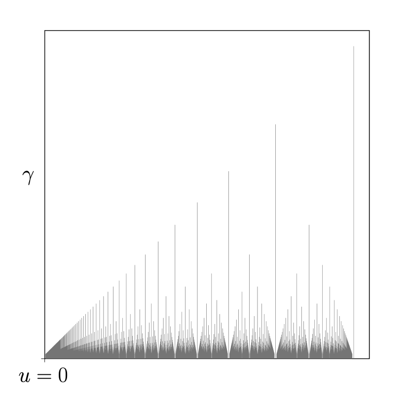
Figure 1. The graph above illustrates a power singularity $\gamma(x,u)$, characterized by pronounced measurement imprecision arising from inherent randomness in the microstructure composition of the material. Despite this inherent uncertainty, our regularity results, applicable both locally and at free boundary points, offer universal and accurate estimates. Remarkably, these estimates remain independent of the substantial oscillations observed in the function $\gamma(x,u)$.

Applying similar reasoning, we can provide examples of energy functionals for which minimizers are locally of class $C^{1,\epsilon}$, for $0<\epsilon\ll 1$, whereas along the free boundary, they are $C^{1,1-\epsilon}-$regular. We anticipate revisiting the analysis of such models in future investigations.

5. Hausdorff measure estimates

In this section, we prove Hausdorff measure estimates for the free boundary under the stronger regularity assumptions on the data

$$\delta(x)\in W^{2,\infty}(B_{1})\quad\mbox{and}\quad\gamma(x)\in W^{2,\infty}(B_{1}).$$ (5.1)

Differentiability of the free boundary will be obtained in Section 7, assuming only $\delta,\gamma\in W^{1,q}(B_{1})$, for some $q>n$.

Furthermore, we shall also assume

$$\gamma^{*}(0,1)\coloneqq\gamma^{*}(B_{1}(0))<1.$$ (5.2)

We will need a few preliminary results, as in [3]. We begin with a slightly different pointwise gradient estimate with respect to Lemma 4.1.

Lemma 5.1.

Let $u$ be a local minimizer of the energy-functional (2.3) in $B_{1}$. Assume (2.13), (4.1), (5.2) and (5.1) are in force and let $x_{0}\in F(u)\cap B_{1/2}$. There exists a constant $c_{1}$, depending only on $n$, $\delta_{0}$, $\gamma_{\star}(0,1)$, $\|D\delta\|_{\infty}$, $\|D^{2}\delta\|_{\infty}$, $\|D\gamma\|_{\infty}$ and $\|D^{2}\gamma\|_{\infty}$, such that

$$|Du(x)|^{2}\leq 2\delta(x)\,[u(x)]^{\gamma(x)}+c_{1}u(x),$$

for each $x\in B_{1/8}(x_{0})$.

Proof.

Consider $\zeta\colon[0,3\tau]\rightarrow\mathbb{R}$, defined by

$$\zeta(t)=\left\{\begin{array}[]{ccl}0&\mathrm{if}&t\in[0,\tau]\\ &&\\ K_{1}\,(t-\tau)^{3}&\mathrm{if}&t\in[\tau,3\tau],\end{array}\right.$$

and define, for $\tau=1/8$ and $K>0$ a large constant to be chosen later,

$$w(y)\coloneqq|Du(y)|^{2}-2\delta(y)[u(y)]^{\gamma(y)}-Ku(y)-\zeta(|y-x_{0}|)[u(y)]^{\gamma(y)},$$

for $y\in\Omega(u)\cap B_{3\tau}(x_{0})$. By Lemma 4.1, we can suitably choose $K_{1}>0$ so that $w\leq 0$ on $\partial B_{3\tau}(x_{0})$, and so $w\leq 0$ on $\partial[\Omega(u)\cap B_{3\tau}(x_{0})]$. We will show that $w\leq 0$ in $\Omega(u)\cap B_{3\tau}(x_{0})$. To do so, we assume, to the contrary, that $w$ attains a positive maximum at $p\in\Omega(u)\cap B_{3\tau}(x_{0})$. Since $w$ is smooth within $\Omega(u)$ and $p$ is a point of maximum for $w$, we have $\Delta w(p)\leq 0$. To reach a contradiction, we will show that $\Delta w(p)>0$, for $\tau$ small and $K$ large.

We will omit the point $p$ whenever possible to ease the notation. We also rotate the coordinate system so that $e_{1}$ is in the direction of $Du(p)$. We then have

$$0 = \partial_{1}w(p)$$

$$= 2Du\cdot D\partial_{1}u-2\partial_{1}\delta u^{\gamma}-2\delta\left(\gamma u^{\gamma-1}\partial_{1}u+\partial_{1}\gamma u^{\gamma}\ln(u)\right)-K\partial_{1}u$$

$$-\partial_{1}\zeta u^{\gamma}-\zeta\left(\gamma u^{\gamma-1}\partial_{1}u+\partial_{1}\gamma\,u^{\gamma}\ln(u)\right)$$

$$= \partial_{1}u\left[2\partial_{11}u-\frac{u^{\gamma}}{\partial_{1}u}(2\partial_{1}\delta+\partial_{1}\zeta)-u^{\gamma-1}\gamma(2\delta+\zeta)-K\right]$$

$$+\partial_{1}u\left[-\frac{u^{\gamma}}{\partial_{1}u}\partial_{1}\gamma\ln(u)(2\delta+\zeta)\right].$$

Since $\partial_{1}u(p)>0$, we obtain

$$2\partial_{11}u=\frac{u^{\gamma}}{\partial_{1}u}(2\partial_{1}\delta+\partial_{1}\zeta)+u^{\gamma-1}\gamma(2\delta+\zeta)+K+\frac{u^{\gamma}}{\partial_{1}u}\partial_{1}\gamma\ln(u)(2\delta+\zeta).$$

Moreover, since $w(p)>0$, it also holds that $\partial_{1}u(p)>\sqrt{2\delta(p)}u(p)^{\frac{\gamma(p)}{2}}$, and so

$$\frac{u^{\gamma}}{\partial_{1}u}\leq\frac{u^{\frac{\gamma}{2}}}{\sqrt{2\delta}}\leq\frac{1}{\sqrt{2\delta_{0}}}u^{\frac{\gamma}{2}}.$$

This implies that

$$2\partial_{11}u\geq 2\delta\gamma u^{\gamma-1}+K+\zeta\gamma u^{\gamma-1}-C_{1}u^{\frac{\gamma}{2}}-C_{2}u^{\frac{\gamma}{2}}|\ln(u)|,$$

for constants $C_{1}=C_{1}(\delta_{0},\|D\delta\|_{\infty},K_{1})$ and $C_{2}=C_{2}(\delta_{0},\|D\gamma\|_{\infty},K_{1})$. For a small $\eta^{*}>0$ so that $\gamma/2-\eta^{*}>0$ and a larger constant $C_{3}$, we then have

$$2\partial_{11}u\geq 2\delta\gamma u^{\gamma-1}+K+\zeta\gamma u^{\gamma-1}-C_{3}u^{\frac{\gamma}{2}-\eta^{*}}.$$

Writing $K=\eta K+(1-\eta)K$, for $\eta\in(0,1)$, we obtain, for large $K$,

$$2\partial_{11}u\geq 2\delta\gamma u^{\gamma-1}+\eta K+\zeta\gamma u^{\gamma-1},$$

and as a consequence, squaring and dropping positive terms,

$$2\left(\partial_{11}u\right)^{2}\geq 2\left(\delta\gamma u^{\gamma-1}\right)^{2}+2\delta\gamma\eta Ku^{\gamma-1}+2\delta\zeta\left(\gamma u^{\gamma-1}\right)^{2}.$$ (5.3)

Now, we calculate $\Delta w$ at the point $p$. By direct computations, we obtain

$$\Delta w = 2\sum_{k,j}(\partial_{k,j}u)^{2}+2Du\cdot D(\Delta u)-2u^{\gamma}\Delta\delta-4D\delta\cdot D(u^{\gamma})$$

$$-2\delta\,\Delta(u^{\gamma})-K\Delta u-u^{\gamma}\Delta\zeta-2D\zeta\cdot D(u^{\gamma})-\zeta\Delta(u^{\gamma}).$$

Moreover,

$$D(u^{\gamma}) = u^{\gamma}\ln(u)D\gamma+\gamma u^{\gamma-1}Du,$$

$$\Delta(u^{\gamma}) = u^{\gamma}\ln(u)\Delta\gamma+u^{\gamma}(\ln(u))^{2}|D\gamma|^{2}+2\gamma u^{\gamma-1}\ln(u)D\gamma\cdot Du$$

$$+2u^{\gamma-1}D\gamma\cdot Du+\gamma(\gamma-1)u^{\gamma-2}|Du|^{2}+\gamma u^{\gamma-1}\Delta u.$$

Observe that, by Lemma 4.1 and since $\gamma<1$,

$$|D(u^{\gamma})|\leq C_{4}\gamma u^{2\gamma-1}.$$

We also have

$$\Delta(u^{\gamma})\leq C_{5}u^{\gamma-1}+\delta\gamma^{2}u^{2\gamma-2}\left[\frac{(\gamma-1)}{\gamma\delta}\frac{|Du|^{2}}{u^{\gamma}}+1\right],$$

for a constant $C_{5}=C_{5}(\|D\gamma\|_{\infty},\|D^{2}\gamma\|_{\infty},\gamma_{\star}(0,1))$. One can now further estimate $\Delta w$ from below to obtain

$$\Delta w \geq \displaystyle 2(\partial_{11}u)^{2}-C_{6}u^{\gamma-1}+2\delta\gamma(\gamma-1)u^{\gamma-2}|Du|^{2}$$

$$\displaystyle-2\delta^{2}\gamma^{2}u^{2\gamma-2}\left[\frac{(\gamma-1)}{\gamma\delta}\frac{|Du|^{2}}{u^{\gamma}}+1\right]-K\delta\gamma u^{\gamma-1}$$

$$\displaystyle-\delta\zeta\gamma^{2}u^{2\gamma-2}\left[\frac{(\gamma-1)}{\gamma\delta}\frac{|Du|^{2}}{u^{\gamma}}+1\right]$$

$$= \displaystyle 2(\partial_{11}u)^{2}-2\delta^{2}\gamma^{2}u^{2\gamma-2}-C_{6}u^{\gamma-1}$$

$$\displaystyle-K\delta\gamma u^{\gamma-1}-\delta\zeta\gamma^{2}u^{2\gamma-2}\left[\frac{(\gamma-1)}{\gamma\delta}\frac{|Du|^{2}}{u^{\gamma}}+1\right].$$

By (5.3), it follows that

$$\Delta w \geq \displaystyle 2\delta\gamma\eta Ku^{\gamma-1}+2\delta\zeta\left(\gamma u^{\gamma-1}\right)^{2}-C_{6}u^{\gamma-1}$$

$$\displaystyle-K\delta\gamma u^{\gamma-1}-\delta\zeta\gamma^{2}u^{2\gamma-2}\left[\frac{(\gamma-1)}{\gamma\delta}\frac{|Du|^{2}}{u^{\gamma}}+1\right]$$

$$= \displaystyle u^{\gamma-1}\left[2\delta\gamma\eta K-C_{6}-K\delta\gamma\right]+2\delta\zeta\left(\gamma u^{\gamma-1}\right)^{2}$$

$$-\displaystyle\delta\zeta\gamma^{2}u^{2\gamma-2}\left[\frac{(\gamma-1)}{\gamma\delta}\frac{|Du|^{2}}{u^{\gamma}}+1\right].$$

Since $\gamma<1$, we conclude

$$\Delta w\geq u^{\gamma-1}\left[2\delta\gamma\eta K-C_{6}-K\delta\gamma\right].$$

Now we fix any $1/2<\eta<1$ and choose $K$ so large that the above expression is positive. This leads to a contradiction, as discussed before. Since $\zeta$ vanishes on $B_{\tau}(x_{0})$, the result is proved. ∎

The second preliminary result concerns the integrability of a negative power of the minimizer.

Lemma 5.2.

Let $u$ be a local minimizer of the energy-functional (2.3) in $B_{1}$. Assume (2.13), (4.1), (5.1) and (5.2) are in force. If $0\in F(u)$, then

$$u(x)^{-\frac{\gamma(x)}{2}}\in L^{1}(\Omega(u)\cap B_{1/2}).$$

Proof.

Observe that it is enough to show that

$$u(x)^{-\frac{\gamma(x)}{2}}\in L^{1}(\Omega(u)\cap B_{\tau}(z)),$$ (5.4)

for some small $\tau>0$ and every $z\in F(u)$. Indeed, once this is proved, we can cover $F(u)\cap B_{1/2}$ with finitely many balls with radius $\tau>0$, say $\{B_{\tau}(z_{i})\}$. Then,

$$\int\limits_{\Omega(u)\cap\left(\cup B_{\tau}(z_{i})\right)}u^{-\frac{\gamma(x)}{2}}\leq\sum_{i}\int\limits_{\Omega(u)\cap B_{\tau}(z_{i})}u^{-\frac{\gamma(x)}{2}}\leq C.$$

Also, by continuity of $u$, we have

$$u\geq c\quad\mbox{in}\quad\left(\Omega(u)\cap B_{1/2}\right)\backslash\cup_{i}B_{\tau}(z_{i}),$$

from which the statement in the lemma follows.

To prove (5.4), we follow closely the argument in [17, Lemma 2.5]. Set

$$w=u^{2-\frac{3}{2}\gamma(x)}.$$

First, take $\rho\in C^{\infty}(\mathbb{R}^{+})$, satisfying $\rho^{\prime}\geq 0$, $\rho\equiv 0$ in $[0,1/2]$ and $\rho(t)=t$ in $[1,\infty)$. For $\delta>0$, let $\rho_{\delta}(t)=\delta\rho(\delta^{-1}t)$. If $\delta<\epsilon$, then

$$\frac{1}{\epsilon}\int_{\{0\leq u<\epsilon\}\cap B_{\tau}(z_{i})}Dw\cdot Du\,\rho_{\delta}^{\prime}(u)=\frac{1}{\epsilon}\int_{B_{\tau}(z_{i})}Dw\cdot D\rho_{\delta}(\min(u,\epsilon))=:A.$$ (5.5)

Integrating by parts, we obtain

$$A=-\frac{1}{\epsilon}\int_{\{0<u\}\cap B_{\tau}(z_{i})}\rho_{\delta}(\min(u,\epsilon))\Delta w+\int_{\partial B_{\tau}(z_{i})}\frac{\rho_{\delta}(\min(u,\epsilon))}{\epsilon}\partial_{\nu}w.$$

Now we choose $\delta=\epsilon/2$, observing that $\rho_{\delta}(u)=0$ in the set $\{0<u\leq\epsilon/4\}$. Therefore,

$$A = \displaystyle-\frac{1}{2}\int_{\{\epsilon/4<u\leq\epsilon\}\cap B_{\tau}(z_{i})}\rho\left(\frac{2}{\epsilon}u\right)\Delta w-\int_{\{\epsilon<u\}\cap B_{\tau}(z_{i})}\Delta w$$

$$+\displaystyle\int_{\partial B_{\tau}(z_{i})}\frac{\rho_{\delta}(\min(u,\epsilon))}{\epsilon}\partial_{\nu}w.$$

By Lemma 4.1, we have

$$|Dw(x)| \leq \displaystyle 2|D\gamma(x)|u(x)^{2-\frac{3}{2}\gamma(x)}\ln(u(x))$$

$$+\displaystyle\left(2-\frac{3}{2}\gamma(x)\right)u(x)^{1-\frac{3}{2}\gamma(x)}|Du(x)|$$

$$\leq \displaystyle C\left(|D\gamma(x)|+1\right),$$

for some universal constant $C>0$, and so

$$A\leq C\tau^{n-1}-\frac{1}{2}\int_{\{\epsilon/4<u\leq\epsilon\}\cap B_{\tau}(z_{i})}\rho\left(\frac{2}{\epsilon}u\right)\Delta w-\int_{\{\epsilon<u\}\cap B_{\tau}(z_{i})}\Delta w.$$ (5.6)

By direct computations, it follows that

$$\Delta w(x) = a(x)+\left(2-\frac{3}{2}\gamma(x)\right)\left(\left(1-\frac{3}{2}\gamma(x)\right)u(x)^{-\frac{3}{2}\gamma(x)}|Du(x)|^{2}\right.$$

$$\qquad\qquad\qquad\qquad\qquad\ \ +u(x)^{1-\frac{3}{2}\gamma(x)}\Delta u(x)\bigg{)},$$

where

$$\frac{2}{3}a(x) = \displaystyle-w(x)\ln(u(x))\Delta\gamma(x)-\ln(u(x))D\gamma(x)\cdot Du(x)$$

$$-\displaystyle 2u(x)^{1-\frac{3}{2}\gamma(x)}D\gamma(x)\cdot Du(x)$$

$$-\displaystyle\left(2-\frac{3}{2}\gamma(x)\right)\ln(u(x))u(x)^{1-\gamma(x)}D\gamma(x)\cdot Du(x).$$

By Lemma 5.1, there exists a universal constant $c>0$ such that

$$\displaystyle\left(\left(1-\frac{3}{2}\gamma(x)\right)u(x)^{-\frac{3}{2}\gamma(x)}|Du(x)|^{2}+u(x)^{1-\frac{3}{2}\gamma(x)}\Delta u(x)\right) =$$

$$\displaystyle u(x)^{\frac{-\gamma(x)}{2}}\,\left(\left(1-\frac{3}{2}\gamma(x)\right)\frac{|Du(x)|^{2}}{u(x)^{\gamma(x)}}+\delta(x)\gamma(x)\right) \geq$$

$$\displaystyle u(x)^{\frac{-\gamma(x)}{2}}\delta(x)\,\left(2(1-\gamma(x))+c(1-g(x))u(x)\right) \geq$$

$$\displaystyle\delta_{0}u(x)^{\frac{-\gamma(x)}{2}}\left(2(1-\gamma^{*}(0,1))-c_{1}\tau^{\frac{2}{2-\gamma(z_{i})}}\right),$$

where, for the last inequality, we used Theorem 4.1. Since $\gamma^{*}(0,1)<1$, we can choose $\tau>0$ small enough, such that

$$2(1-\gamma^{*}(0,1))-c_{1}\tau^{\frac{2}{2-\gamma(z_{i})}}\geq(1-\gamma^{*}(0,1)),$$

and so

$$\Delta w(x)\geq a(x)+c_{2}u(x)^{-\frac{\gamma(x)}{2}}.$$

Furthermore, notice that

$$|a(x)|\leq C(|D\gamma(x)|+|D^{2}\gamma(x)|+1),$$

for some positive universal constant $C>0$. Therefore, by (5.6), we have

$$A \leq \displaystyle-\frac{1}{2}\int_{\{\epsilon/4<u\leq\epsilon\}\cap B_{\tau}(z_{i})}\rho\left(\frac{2}{\epsilon}u\right)\left(a(x)+c_{2}u(x)^{-\frac{\gamma(x)}{2}}\right)$$

$$-\displaystyle\int_{\{\epsilon<u\}\cap B_{\tau}(z_{i})}\left(a(x)+c_{2}u(x)^{-\frac{\gamma(x)}{2}}\right)$$

$$\leq \displaystyle C\left(\|D\gamma\|_{L^{1}},\|D^{2}\gamma\|_{L^{1}}\right)-\overline{c}\int_{\{\epsilon/4<u\}\cap B_{\tau}(z_{i})}u(x)^{-\frac{\gamma(x)}{2}}.$$

Now, we estimate the left-hand side of (5.5). By Lemma 4.1 and since $\gamma^{*}(0,1)<1$, we obtain

$$Dw\cdot Du \geq -2u(x)^{2-\frac{3}{2}\gamma(x)}|\ln(u(x))||D\gamma(x)|\,|Du(x)|$$

$$\geq -Cu(x)^{2-\gamma(x)}|\ln(u(x))||D\gamma(x)|$$

$$\geq -Cu(x)^{2-\gamma^{*}(0,1)}|\ln(u(x))||D\gamma(x)|$$

$$\geq -C_{1}u(x)\,|D\gamma(x)|,$$

for some universal constant $C_{1}$. Thus, from (5.5), we have

$$-C_{1}\frac{1}{\epsilon}\int_{\{0\leq u<\epsilon\}\cap B_{\tau}(z_{i})}u(x)|D\gamma(x)|\,\rho_{\delta}^{\prime}(u)$$

$$\leq C\left(\|D\gamma\|_{L^{1}},\|D^{2}\gamma\|_{L^{1}}\right)-\overline{c}\int_{\{\epsilon/4<u\}\cap B_{\tau}(z_{i})}u(x)^{-\frac{\gamma(x)}{2}}.$$

Since $\rho_{\delta}^{\prime}\leq 1$, we obtain

$$\int_{\{\epsilon/4<u\}\cap B_{\tau}(z_{i})}u(x)^{-\frac{\gamma(x)}{2}}\leq C\left(\overline{c},C_{1},\|D\gamma\|_{L^{1}},\|D^{2}\gamma\|_{L^{1}}\right).$$

We get the result by passing to the limit as $\epsilon\rightarrow 0$. ∎

We are now ready to state and prove the main result of this section.

Theorem 5.1.

Let $u$ be a local minimizer of the energy-functional (2.3) in $B_{1}$. Assume (2.13), (4.1), (5.1) and (5.2) are in force. Then, there exists a universal constant $C>0$, depending only on $n$, $\delta_{0}$, $\gamma_{\star}(0,1)$, $\|D\delta\|_{\infty}$, $\|D^{2}\delta\|_{\infty}$, $\|D\gamma\|_{\infty}$ and $\|D^{2}\gamma\|_{\infty}$, such that

$$\mathcal{H}^{n-1}(F(u)\cap B_{1/2})<C.$$

Proof.

Assume $0\in F(u)$. It is enough to prove that for some small $r$,

$$\mathcal{H}^{n-1}(F(u)\cap B_{r})<\infty.$$

Given a small parameter $\epsilon>0$, we cover $F(u)\cap B_{r}$ with finitely many balls $\{B_{\epsilon}(x_{i})\}_{i\in F_{\epsilon}}$ with finite overlap, that is,

$$\sum_{i\in F_{\epsilon}}\mathcal{X}_{B_{\epsilon}(x_{i})}\leq c,$$

for a constant $c>0$ that depends only on the dimension $n$. It then follows that

$$\mathcal{H}^{n-1}(F(u)\cap B_{r})\leq\overline{c}\liminf_{\epsilon\rightarrow 0}\epsilon^{n-1}\#(F_{\epsilon}).$$

Since $x_{i}\in F(u)$, by Theorem 4.1, we have

$$\Omega(u)\cap B_{\epsilon}(x_{i})\subset\left\{0<u\leq\overline{M}\epsilon^{\beta_{i}}\right\}\cap B_{\epsilon}(x_{i}),$$

where $\beta_{i}=2/(2-\gamma(x_{i}))$. By assumption (4.1), it follows that

$$\Omega(u)\cap B_{\epsilon}(x_{i})\subset\left\{0<u\leq\overline{M}_{1}\epsilon^{\beta^{*}(x_{i},\epsilon)}\right\}\cap B_{\epsilon}(x_{i}),$$

for a universal constant $\overline{M}_{1}>\overline{M}$. Let us assume, to simplify, that $\overline{M}_{1}=1$. Now, observe that

$$\bigcup_{i\in F_{\epsilon}}\left(B_{\epsilon}(x_{i})\cap\left\{0<u(x)\leq\epsilon^{\beta^{*}(x_{i},\epsilon)}\right\}\right)\subseteq B_{2r}\cap\left\{0<u(x)^{\frac{1}{\beta(x)}}<\epsilon\right\}.$$

Since the covering $\{B_{\epsilon}(x_{i})\}_{i\in F_{\epsilon}}$ has finite overlap, it then follows that

$$\sum_{i\in F_{\epsilon}}\left|\Omega(u)\cap B_{\epsilon}(x_{i})\right|\leq c\left|B_{2r}\cap\left\{0<u(x)^{\frac{1}{\beta(x)}}<\epsilon\right\}\right|.$$

By Theorem 4.3, this implies that

$$|\Omega(u)\cap B_{\epsilon}(x_{i})|\geq\mu_{0}\epsilon^{n},$$

and so

$$\epsilon^{n-1}\#(F_{\epsilon})\leq\frac{c}{\mu_{0}}\frac{\left|B_{2r}\cap\left\{0<u(x)^{\frac{1}{\beta(x)}}<\epsilon\right\}\right|}{\epsilon},$$

which readily leads to

$$\mathcal{H}^{n-1}(F(u)\cap B_{r})\leq\frac{\overline{c}\,c}{\mu_{0}}\liminf_{\epsilon\rightarrow 0}\frac{|\left|B_{2r}\cap\left\{0<u(x)^{\frac{1}{\beta(x)}}<\epsilon\right\}\right|}{\epsilon}.$$

We will show below that the right-hand side of the inequality above can be bounded above uniformly in $\epsilon$. To do so, let

$$v(x)\coloneqq u(x)^{\frac{1}{\beta(x)}}.$$

Observe that

$$\int\limits_{B_{2r}\cap\{0<v\leq\epsilon\}}|Dv|^{2}=\int\limits_{B_{2r}}D(\min(v,\epsilon))\cdot Dv=:I.$$

Integrating by parts, we get

$$I=-\int\limits_{B_{2r}}\min(v,\epsilon)\Delta v+\int\limits_{\partial B_{2r}}\min(v,\epsilon)\partial_{\nu}v,$$

and so,

$$\int\limits_{B_{2r}\cap\{0<v\leq\epsilon\}}|Dv|^{2}+v\Delta v=-\epsilon\int\limits_{B_{2r}\cap\{v>\epsilon\}}\Delta v+\int\limits_{\partial B_{2r}}\min(v,\epsilon)\partial_{\nu}v.$$ (5.7)

By direct computations, we readily obtain

$$Dv(x)=g(x)D\left(\frac{1}{\beta(x)}\right)+\frac{1}{\beta(x)}u(x)^{\frac{1}{\beta(x)}-1}Du(x)$$

and

$$\Delta v(x)=A(x)+B(x)+\frac{\delta(x)\,\gamma(x)}{\beta(x)}u(x)^{-\frac{1}{\beta(x)}},$$

where $g(x)=v(x)\ln(u(x))$, with

$$A(x) = g(x)\Delta\left(\frac{1}{\beta(x)}\right)+D\left(\frac{1}{\beta(x)}\right)\cdot Dg(x)$$

$$+u(x)^{\frac{1}{\beta(x)}-1}\,D\left(\frac{1}{\beta(x)}\right)\cdot Du(x),$$

and

$$B(x)=\frac{1}{\beta(x)}D\left(u^{\frac{1}{\beta(x)}-1}\right)\cdot Du(x).$$

Let us first bound (5.7) from below. To do so, we estimate

$$|Dv|^{2}+v\Delta v = \displaystyle g(x)^{2}\left|D\left(\frac{1}{\beta(x)}\right)\right|^{2}+\frac{1}{\beta(x)^{2}}u(x)^{2\left(\frac{1}{\beta(x)}-1\right)}|Du|^{2}$$

$$+2\frac{1}{\beta(x)}g(x)D\left(\frac{1}{\beta(x)}\right)\cdot Du(x)$$

$$+(A(x)+B(x))u(x)^{\frac{1}{\beta(x)}}+\frac{\delta(x)\,\gamma(x)}{\beta(x)}$$

$$\geq B(x)u(x)^{\frac{1}{\beta(x)}}+\frac{1}{\beta(x)^{2}}u(x)^{2\left(\frac{1}{\beta(x)}-1\right)}|Du|^{2}$$

$$+2\frac{1}{\beta(x)}g(x)D\left(\frac{1}{\beta(x)}\right)\cdot Du(x)$$

$$+A(x)u(x)^{\frac{1}{\beta(x)}}+\frac{\delta_{0}\,\gamma_{\star}(0,1)}{2}.$$

By Lemma 4.1, we have

$$B(x)u(x)^{\frac{1}{\beta(x)}}+\frac{1}{\beta(x)^{2}}u(x)^{2\left(\frac{1}{\beta(x)}-1\right)}|Du|^{2}\qquad\qquad\qquad$$

$$\geq \frac{1}{\beta(x)}u^{\frac{2}{\beta(x)}-1}\ln(u(x))D\left(\frac{1}{\beta(x)}\right)\cdot Du(x)$$

$$\geq -u(x)^{\frac{1}{\beta(x)}}\ln(u(x))|D\gamma(x)|$$

$$\geq -u^{\frac{1}{2\beta(x)}}|D\gamma(x)|,$$

which implies

$$|Dv|^{2}+v\Delta v \geq \displaystyle-Cu^{\frac{1}{2\beta(x)}}|D\gamma(x)|$$

$$+2\frac{1}{\beta(x)}g(x)D\left(\frac{1}{\beta(x)}\right)\cdot Du(x)$$

$$+A(x)u(x)^{\frac{1}{\beta(x)}}+\frac{\delta_{0}\,\gamma_{\star}(0,1)}{2},$$

for some universal constant $C$. Using Lemma 4.1 once more, we can show that

$$\left|2\frac{1}{\beta(x)}g(x)D\left(\frac{1}{\beta(x)}\right)\cdot Du(x)\right|\leq C_{1}u(x)^{\frac{1}{\beta(x)}}|D\gamma(x)|$$

and

$$|A(x)|\leq C_{1}(|D\gamma(x)|+|D^{2}\gamma(x)|+|D\gamma(x)||\ln(u(x))|),$$

for some universal constant $C_{1}$, and so

$$|Dv|^{2}+v\Delta v \geq \displaystyle-C_{2}u^{\frac{1}{2\beta(x)}}|D\gamma(x)|-C_{1}u^{\frac{1}{\beta(x)}}\left(|D\gamma(x)|+|D^{2}\gamma(x)|\right)$$

$$+\frac{\delta_{0}\,\gamma_{\star}(0,1)}{2},$$

for a universal constant $C_{2}$. We can now estimate the left-hand side of (5.7) as

$$\int\limits_{B_{2r}\cap\{0<v\leq\epsilon\}}|Dv|^{2}+v\Delta v \geq \displaystyle-C_{2}\|D\gamma\|_{\infty}\epsilon^{1/2}|B_{2r}\cap\{0<v\leq\epsilon\}|$$

$$-C_{1}\epsilon(\|D\gamma\|_{L^{1}(B_{2r})}+\|D^{2}\gamma\|_{L^{1}(B_{2r})})$$

$$+\frac{\delta_{0}\,\gamma_{\star}(0,1)}{2}|B_{2r}\cap\{0<v\leq\epsilon\}|$$

$$\geq \frac{\delta_{0}\,\gamma_{\star}(0,1)}{4}|B_{2r}\cap\{0<v\leq\epsilon\}|-C_{3}\epsilon,$$

for $\epsilon$ small enough and depending only on universal constants. By Lemma 4.1, there exists a constant $C_{4}>0$ such that $|Dv|\leq C_{4}$, and so (5.7) implies

$$\frac{\delta_{0}\,\gamma_{\star}(0,1)}{4}|B_{2r}\cap\{0<v\leq\epsilon\}|-C_{2}\epsilon\leq-\epsilon\int\limits_{B_{2r}\cap\{v>\epsilon\}}\Delta v+C_{4}\epsilon,$$

and so

$$\frac{\delta_{0}\,\gamma_{\star}(0,1)}{4}\frac{|B_{2r}\cap\{0<v\leq\epsilon\}|}{\epsilon}\leq C_{2}+C_{4}-\int\limits_{B_{2r}\cap\{v>\epsilon\}}\Delta v.$$

The proof will then be complete as long as this remaining integral is uniformly bounded in $\epsilon>0$. Recalling the expression for $\Delta v$, we have

$$-\Delta v \leq \displaystyle|A(x)|+B(x)+\frac{\delta(x)\,\gamma(x)}{\beta(x)}u(x)^{-\frac{1}{\beta(x)}}$$

$$\leq C_{1}(|D\gamma(x)|+|D^{2}\gamma(x)|+|D\gamma(x)||\ln(u(x))|)$$

$$+u(x)^{-\frac{\gamma(x)}{2}}\left(\frac{1}{2}\ln(u(x))D\gamma(x)\cdot Du(x)+\frac{\gamma(x)}{2}\frac{1}{u(x)}|Du(x)|^{2}\right)$$

$$-\frac{\delta(x)\,\gamma(x)}{\beta(x)}u(x)^{-\frac{1}{\beta(x)}}$$

$$\leq C_{5}(|D\gamma(x)|+|D^{2}\gamma(x)|)+C_{6}|D\gamma(x)||\ln(u(x))|+C_{7}u(x)^{-\frac{\gamma(x)}{2}}$$

$$\leq C_{5}(|D\gamma(x)|+|D^{2}\gamma(x)|)+C_{8}|D\gamma|_{\infty}u(x)^{-\frac{\gamma(x)}{2}},$$

where we used Lemma 5.1 and the fact that $|\ln(u(x))|$ can be bounded above by $u(x)^{-\frac{\gamma(x)}{2}}$. This implies that

$$\int\limits_{B_{2r}\cap\{v>\epsilon\}}\Delta v\leq C_{5}(\|D\gamma\|_{L^{1}}+\|D^{2}\gamma\|_{L^{1}})+C_{8}|D\gamma|_{\infty}+\int\limits_{B_{2r}\cap\{v>\epsilon\}}u(x)^{-\frac{\gamma(x)}{2}},$$

from which the conclusion of the theorem follows in view of Lemma 5.2. ∎

6. Monotonicity formula and classification of blow-ups

In this section, we obtain a monotonicity formula valid for local minimizers of the energy-functional (2.3). Given $z_{0}\in B_{1}$, let

$$\gamma\coloneqq\gamma(z_{0})\qquad\mbox{and}\qquad\beta\coloneqq\frac{2}{2-\gamma}.$$

Now, for a Lipschitz function $v$ and $z_{0}\in F(v)$, define

$$\displaystyle W_{v,z_{0}}(r) := \displaystyle r^{-(n+2(\beta-1))}\int\limits_{B_{r}(z_{0})}\frac{1}{2}|Dv|^{2}+\delta(x)v^{\gamma(x)}\chi_{\{v>0\}}$$ (6.1)

$$-\beta r^{-((n-1)+2\beta)}\int\limits_{\partial B_{r}(z_{0})}v^{2}$$

$$-\int_{0}^{r}\beta t^{-(n+\beta\gamma+1)}\int\limits_{B_{t}(z_{0})}(\gamma(x)-\gamma)\delta(x)v^{\gamma(x)}\chi_{\{v>0\}}$$

$$-\int_{0}^{r}t^{-(n+\beta\gamma+1)}\int\limits_{B_{t}(z_{0})}\left(D\gamma(x)\cdot(x-z_{0})\right)\delta(x)v^{\gamma(x)}\ln(v)\chi_{\{v>0\}}$$

$$-\int_{0}^{r}t^{-(n+\beta\gamma+1)}\int\limits_{B_{t}(z_{0})}(D\delta(x)\cdot(x-z_{0}))v^{\gamma(x)}\chi_{\{v>0\}}.$$

For our formula to hold, we will further need to assume that, for some $0<r_{0}<1$,

$$t\rightarrow t^{-n}\int_{B_{t}(z_{0})}|D\delta(x)|dx\in L^{1}(0,r_{0})$$ (6.2)

and

$$t\rightarrow t^{-n}\ln t\int_{B_{t}(z_{0})}|D\gamma(x)|dx\in L^{1}(0,r_{0}).$$ (6.3)

We remark that sufficient conditions for these to hold are $|D\delta|\in L^{q}(B_{1})$ and $|D\gamma|\in L^{q}(B_{1})$, for $q>n$. Indeed, we readily have

$$t^{-n}\ln t\int_{B_{t}(z_{0})}|D\gamma(x)|dx\leq C(n,q)\|D\gamma\|_{L^{q}\left(B_{r_{0}}(z_{0})\right)}\,t^{-\frac{n}{q}}\ln t,$$

and

$$\int_{0}^{r_{0}}t^{-\frac{n}{q}}\ln t\,dt<\infty\quad\Longleftarrow\quad q>n.$$

Remark 6.1.

If we assume $\gamma\in W^{1,q}$, for $q>n$, then $\gamma$ is Hölder continuous and therefore condition (4.1) is automatically satisfied. We also point out that these integrability conditions are important to assure that $W_{u,z_{0}}(r)<\infty$, for every $0<r$ and $z_{0}\in F(u)$ such that $B_{r}(z_{0})\Subset B_{1}$, for $u$ a local minimizer of (2.3).

We are now ready to state and prove the monotonicity formula for local minimizers of our oscillatory exponent functional.

Theorem 6.1.

Let $u$ be a local minimizer of (2.3) and assume (6.2) and (6.3) are in force. If $z_{0}\in F(u)$, then

$$\frac{d}{dr}W_{u,z_{0}}(r)\geq 0.$$

Proof.

Without loss of generality, we consider $z_{0}=0$. Let

$$\overline{W}_{u}(r) = r^{-(n+2(\beta-1))}\int_{B_{r}}\frac{1}{2}|Du|^{2}+\delta(x)\,u^{\gamma(x)}\chi_{\{u>0\}}$$

$$-\beta r^{-((n-1)+2\beta)}\int_{\partial B_{r}}u^{2},$$

and define

$$u_{r}(x)\coloneqq\frac{u(rx)}{r^{\beta}}\quad\mbox{and}\quad\gamma_{r}(x)\coloneqq\gamma(rx).$$

By scaling,

$$\overline{W}_{u}(r)=\int_{B_{1}}\frac{1}{2}|Du_{r}|^{2}+\delta(rx)\,r^{\beta(\gamma_{r}(x)-\gamma)}u_{r}^{\gamma_{r}(x)}\chi_{\{u_{r}>0\}}-\beta\int_{\partial B_{1}}u_{r}^{2},$$

where we used that, by definition of the parameter $\beta$, we have

$$2(\beta-1)=\beta\gamma.$$

Differentiating $\overline{W}_{u}$ with respect to $r$ leads to

$$\frac{d}{dr}\overline{W}_{u}(r) = \displaystyle\int_{B_{1}}Du_{r}\cdot D\left(\frac{d}{dr}u_{r}\right)+\frac{d}{dr}\left(\delta(rx)\,r^{\beta(\gamma_{r}(x)-\gamma)}u_{r}^{\gamma_{r}(x)}\right)\chi_{\{u_{r}>0\}}$$

$$-\beta\int_{\partial B_{1}}2u_{r}\frac{d}{dr}u_{r}.$$

Integrating by parts, we obtain

$$\frac{d}{dr}\overline{W}_{u}(r)=(A)+(B)+(C)+(D)+(E),$$

for

$$(A) \coloneqq \displaystyle\int_{B_{1}}-\Delta u_{r}\cdot\frac{d}{dr}u_{r},$$

$$(B) \coloneqq \displaystyle 2\int_{\partial B_{1}}(\partial_{\nu}u_{r}-\beta u_{r})\frac{d}{dr}u_{r},$$

$$(C) \coloneqq \displaystyle\int_{B_{1}}\frac{d}{dr}\left(r^{\beta(\gamma_{r}(x)-\gamma)}\right)\delta(rx)\,u_{r}^{\gamma_{r}(x)}\chi_{\{u_{r}>0\}},$$

$$(D) \coloneqq \displaystyle\int_{B_{1}}r^{\beta(\gamma_{r}(x)-\gamma)}\delta(rx)\,\frac{d}{dr}\left(u_{r}^{\gamma_{r}(x)}\right)\chi_{\{u_{r}>0\}},$$

$$(E) \coloneqq \displaystyle\int_{B_{1}}\left(D\delta(rx)\cdot x\right)\,r^{\beta(\gamma_{r}(x)-\gamma)}u_{r}^{\gamma_{r}}\chi_{\{u_{r}>0\}}.$$

In order to simplify the notation, we write $\gamma_{r}=\gamma_{r}(x)$ and notice that

$$(D) = \displaystyle\int_{B_{1}}r^{\beta(\gamma_{r}-\gamma)}\delta(rx)\,\left(\gamma_{r}u_{r}^{\gamma_{r}-1}\frac{d}{dr}u_{r}+u_{r}^{\gamma_{r}}\ln(u_{r})\frac{d}{dr}\gamma_{r}\right)\chi_{\{u_{r}>0\}}$$

$$= (D.1)+(D.2).$$

Since $u$ is a minimizer to (2.3), it follows that $(D.1)+(A)=0$, and so

$$\frac{d}{dr}\overline{W}_{u}(r)=(B)+(C)+(D.2)+(E).$$

By direct computations, it follows that

$$\frac{d}{dr}u_{r}(x)=r^{-\beta}\left(Du(rx)\cdot x-\beta r^{\beta-1}u_{r}(x)\right).$$

Since $\nu$ is the normal vector at $\partial B_{1}$, we obtain

$$\partial_{\nu}u_{r}(x)=r^{1-\beta}\partial_{\nu}u(rx)=r^{1-\beta}Du(rx)\cdot x,$$

which implies that

$$\frac{d}{dr}u_{r}=\frac{1}{r}\left(\partial_{\nu}u_{r}-\beta u_{r}\right).$$

Hence,

$$(B)=\frac{2}{r}\int_{\partial B_{1}}|\partial_{\nu}u_{r}-\beta u_{r}|^{2}.$$

Moreover,

$$(C) = \displaystyle\int_{B_{1}}\beta(\gamma_{r}-\gamma)r^{\beta(\gamma_{r}-\gamma)-1}\delta(rx)\,u_{r}^{\gamma_{r}}\chi_{\{u_{r}>0\}}$$

$$+\int_{B_{1}}r^{\beta(\gamma_{r}-\gamma)}\beta\ln(r)\delta(rx)\,u_{r}^{\gamma_{r}}\left(\frac{d}{dr}\gamma_{r}\right)\chi_{\{u_{r}>0\}},$$

and

$$(D.2)=\displaystyle\int_{B_{1}}r^{\beta(\gamma_{r}-\gamma)}\delta(rx)\,u_{r}^{\gamma_{r}}\left(\ln(u(rx))-\beta\ln(r)\right)\left(\frac{d}{dr}\gamma_{r}\right)\chi_{\{u_{r}>0\}}.$$

Therefore,

$$(C)+(D.2) = \displaystyle r^{-(n+\beta\gamma+1)}\int_{B_{r}}\beta(\gamma(x)-\gamma)\delta(x)u^{\gamma(x)}\chi_{\{u>0\}}$$

$$+r^{-(n+\beta\gamma+1)}\int_{B_{r}}\delta(x)\ln(u)u^{\gamma(x)}(D\gamma(x)\cdot x)\chi_{\{u>0\}}.$$

This implies that

$$\frac{d}{dr}\overline{W}_{u}(r) = \displaystyle\frac{2}{r}\int_{\partial B_{1}}|\partial_{\nu}u_{r}-\beta u_{r}|^{2}$$

$$+r^{-(n+\beta\gamma+1)}\int_{B_{r}}\beta(\gamma(x)-\gamma)\delta(x)u^{\gamma(x)}\chi_{\{u>0\}}$$

$$+r^{-(n+\beta\gamma+1)}\int_{B_{r}}\delta(x)\ln(u)u^{\gamma(x)}(D\gamma(x)\cdot x)\chi_{\{u>0\}}$$

$$+r^{-(n+\beta\gamma+1)}\int_{B_{r}}(D\delta(x)\cdot x)u^{\gamma(x)}\chi_{\{u>0\}}.$$

Now, recalling the definition of $W_{u,0}(r)$, we have

$$\frac{d}{dr}W_{u,0}(r) = \displaystyle\frac{d}{dr}\overline{W}_{u}(r)-r^{-(n+\beta\gamma+1)}\int_{B_{r}}\beta(\gamma(x)-\gamma)\delta(x)u^{\gamma(x)}\chi_{\{u>0\}}$$

$$-r^{-(n+\beta\gamma+1)}\int_{B_{r}}\delta(x)\ln(u)u^{\gamma(x)}(D\gamma(x)\cdot x)\chi_{\{u>0\}}$$

$$-r^{-(n+\beta\gamma+1)}\int_{B_{r}}(D\delta(x)\cdot x)u^{\gamma(x)}\chi_{\{u>0\}},$$

which implies, by our previous computations, that

$$\frac{d}{dr}W_{u,0}(r)=\frac{2}{r}\int_{\partial B_{1}}|\partial_{\nu}u_{r}-\beta u_{r}|^{2}\geq 0.$$

∎

As a consequence of the monotonicity formula, we obtain the homogeneity of blow-ups.

Definition 6.1 (Blow-up).

Given a point $z_{0}\in F(u)$, we say that $u_{0}$ is a blow-up of $u$ at $z_{0}$ if the family $\{u_{r}\}_{r>0}$, defined by

$$u_{r}(x)\coloneqq\frac{u(z_{0}+rx)}{r^{\beta(z_{0})}},\quad\mbox{with}\quad\beta(z_{0})\coloneqq\frac{2}{2-\gamma(z_{0})},$$

converges, through a subsequence, to $u_{0}$, when $r\to 0$.

We say $u_{0}$ is $\beta(z_{0})$-homogeneous if

$$u_{0}(\lambda x)=\lambda^{\beta(z_{0})}u_{0}(x),\quad\forall\lambda>0,\ \forall x\in\mathbb{R}^{n}.$$

Unlike in the constant case $\gamma(x)\equiv\gamma_{0}$, the homogeneity property of blow-ups will vary depending on the free boundary point we are considering. This is the object of the following result.

Corollary 6.1.

Let $u$ be a local minimizer of (2.3) and assume (6.2) and (6.3) are in force. If $u_{0}$ is a blow-up of $u$ at a point $z_{0}\in F(u)\cap B_{1/2}$, then $u_{0}$ is $\beta(z_{0})$-homogeneous.

Proof.

Without loss of generality, we assume $z_{0}=0$. Recall

$$\beta\coloneqq\frac{2}{2-\gamma}\quad\mbox{where}\quad\gamma\coloneqq\gamma(0).$$

In order to ease the notation, for each $j\in\mathbb{N}$, we will write $\gamma_{j}$ instead of $\gamma(\lambda_{j}x)$, and define

$$W_{v}^{j}(r) := r^{-(n+2(\beta-1))}\int_{B_{r}}\frac{1}{2}|Dv|^{2}+\lambda_{j}^{\beta(\gamma_{j}-\gamma)}v^{\gamma_{j}}\delta(\lambda_{j}x)\chi_{\{v>0\}}$$

$$- \beta r^{-((n-1)+2\beta)}\int_{\partial B_{r}}v^{2}$$

$$- \int_{0}^{r}\beta t^{-(n+\beta\gamma+1)}\int_{B_{t}}(\gamma_{j}-\gamma)\lambda_{j}^{\beta(\gamma_{j}-\gamma)}\delta(\lambda_{j}x)v^{\gamma_{j}}\chi_{\{v>0\}}$$

$$- \int_{0}^{r}t^{-(n+\beta\gamma+1)}\int_{B_{t}}\left(D\gamma(\lambda_{j}x)\cdot x\right)\lambda_{j}^{\beta(\gamma_{j}-\gamma)+1}\delta(\lambda_{j}x)v^{\gamma_{j}}\ln(\lambda_{j}^{\beta}v)\chi_{\{v>0\}}$$

$$- \int_{0}^{r}t^{-(n+\beta\gamma+1)}\int_{B_{t}}\left(D\delta(\lambda_{j}x)\cdot x\right)\lambda_{j}^{\beta(\gamma_{j}-\gamma)+1}v^{\gamma_{j}}\chi_{\{v>0\}}$$

and

$$W^{\infty}_{v}(r):=r^{-(n+2(\beta-1))}\int_{B_{r}}\frac{1}{2}|Dv|^{2}+\delta(0)v^{\gamma(0)}\chi_{\{v>0\}}-\beta r^{-((n-1)+2\beta)}\int_{\partial B_{r}}v^{2}.$$

We now show that

$$W^{\infty}_{u_{0}}(r)=\lim_{j\rightarrow\infty}W^{j}_{u_{j}}(r)\quad\mbox{as long as}\quad\lim_{j\rightarrow\infty}\lambda_{j}^{\beta(\gamma_{j}-\gamma)}\rightarrow 1.$$

Indeed,

$$W_{u_{j}}^{j}(r) = r^{-(n+2(\beta-1))}\int_{B_{r}}\frac{1}{2}|Du_{j}|^{2}+\lambda_{j}^{\beta(\gamma_{j}-\gamma)}\delta(\lambda_{j}x)u_{j}^{\gamma_{j}}\chi_{\{u_{j}>0\}}$$

$$-\beta r^{-((n-1)+2\beta)}\int_{\partial B_{r}}u_{j}^{2}$$

$$-\int_{0}^{r}\beta t^{-(n+\beta\gamma+1)}\int_{B_{t}}(\gamma_{j}-\gamma)\lambda_{j}^{\beta(\gamma_{j}-\gamma)}\delta(\lambda_{j}x)u_{j}^{\gamma_{j}}\chi_{\{u_{j}>0\}}$$

$$-\int_{0}^{r}t^{-(n+\beta\gamma+1)}\int_{B_{t}}\left(D\gamma(\lambda_{j}x)\cdot x\right)\lambda_{j}^{\beta(\gamma_{j}-\gamma)+1}\delta(\lambda_{j}x)u_{j}^{\gamma_{j}}\ln(u(\lambda_{j}x))\chi_{\{u_{j}>0\}}$$

$$-\int_{0}^{r}t^{-(n+\beta\gamma+1)}\int_{B_{t}}\left(D\delta(\lambda_{j}x)\cdot x\right)\lambda_{j}^{\beta(\gamma_{j}-\gamma)+1}u_{j}^{\gamma_{j}}\chi_{\{u_{j}>0\}}$$

and scaling back to $u$, we obtain

$$W_{u_{j}}^{j}(r) = (\lambda_{j}r)^{-(n+2(\beta-1))}\int_{B_{\lambda_{j}r}}\frac{1}{2}|Du|^{2}+\delta(x)u^{\gamma(x)}\chi_{\{u>0\}}$$

$$-\beta(\lambda_{j}r)^{-((n-1)+2\beta)}\int_{\partial B_{\lambda_{j}r}}u^{2}$$

$$-\int_{0}^{r}\beta t^{-(n+\beta\gamma+1)}\lambda_{j}^{-(n+\beta\gamma)}\int_{B_{\lambda_{j}t}}(\gamma(x)-\gamma)\delta(x)u^{\gamma(x)}\chi_{\{u>0\}}$$

$$-\int_{0}^{r}t^{-(n+\beta\gamma+1)}\lambda_{j}^{-(n+\beta\gamma)}\int_{B_{\lambda_{j}t}}\left(D\gamma(x)\cdot x\right)\delta(x)u^{\gamma(x)}\ln\left(u(x)\right)\chi_{\{u>0\}}$$

$$-\int_{0}^{r}t^{-(n+\beta\gamma+1)}\lambda_{j}^{-(n+\beta\gamma)}\int_{B_{\lambda_{j}t}}\left(D\delta(x)\cdot x\right)u^{\gamma(x)}\chi_{\{u>0\}}.$$

Changing variables in the last three integrals, we reach

$$W^{j}_{u_{j}}(r) = \displaystyle(\lambda_{j}r)^{-(n+2(\beta-1))}\int_{B_{\lambda_{j}r}}\frac{1}{2}|Du|^{2}+\delta(x)u^{\gamma(x)}\chi_{\{u>0\}}$$

$$-\beta(\lambda_{j}r)^{-((n-1)+2\beta)}\int_{\partial B_{\lambda_{j}r}}u^{2}$$

$$-\int_{0}^{\lambda_{j}r}\beta t^{-(n+\beta\gamma+1)}\int_{B_{t}}(\gamma(x)-\gamma)\delta(x)u^{\gamma(x)}\chi_{\{u>0\}}$$

$$-\int_{0}^{\lambda_{j}r}t^{-(n+\beta\gamma+1)}\int_{B_{t}}\left(D\gamma(x)\cdot x\right)\delta(x)u^{\gamma(x)}\ln(u)\chi_{\{u>0\}}$$

$$-\int_{0}^{\lambda_{j}r}t^{-(n+\beta\gamma+1)}\int_{B_{t}}\left(D\delta(x)\cdot x\right)u^{\gamma(x)}\chi_{\{u>0\}},$$

and so

$$W^{j}_{u_{j}}(r)=W_{u}(\lambda_{j}r).$$

Therefore

$$W^{\infty}_{u_{0}}(r)=\lim_{j\rightarrow\infty}W^{j}_{u_{j}}(r)=\lim_{j\rightarrow\infty}W_{u}(\lambda_{j}r)=W_{u}(0^{+}),$$

where the last inequality is guaranteed by the monotonicity of the functional at the minimizer $u$. We conclude that $W^{\infty}_{u_{0}}$ is constant. We note that $u_{0}$ is a minimizer to the functional

$$\int_{B_{R}}\frac{1}{2}|Dv|^{2}+\delta(0)v^{\gamma(0)}\chi_{\{v>0\}},$$ (6.4)

for every $R>0$, and thus entitled to the regularity results from [3]. In particular, it follows, from [3, Lemma 7.1], that $u_{0}$ is $\beta(0)$-homogeneous. ∎

Remark 6.2.

To assure the existence of blow-ups, one needs to guarantee that the family $(u_{r})_{r>0}$, defined as

$$u_{r}(x)=\frac{u(z_{0}+rx)}{r^{\beta(z_{0})}}\quad\mbox{for}\quad\beta(z_{0})=\frac{2}{2-\gamma(z_{0})},$$

is locally bounded in $C^{1,\beta(z_{0})-1}$. Indeed, by Theorem 4.1, there exists a constant $C^{\prime}>1$ such that

$$\|u_{r}\|_{L^{\infty}(B_{1})}\leq C^{\prime}.$$

Moreover, by applying Theorem 2.1 to $u$ over $B_{r}(z_{0})$, we obtain

$${\mathrm{osc}}_{B_{r}(z_{0})}|Du|\coloneqq\left(\sup_{B_{r}(z_{0})}|Du|\right)-\left(\inf_{B_{r}(z_{0})}|Du|\right)\leq Cr^{\frac{\gamma_{\ast}(z_{0},2r)}{2-\gamma_{\ast}(z_{0},2r)}}.$$

Proceeding as at the end of the proof of Theorem 4.1, we use condition (4.1) to obtain

$$Cr^{\frac{\gamma_{\ast}(z_{0},2r)}{2-\gamma_{\ast}(z_{0},2r)}}\leq\overline{C}r^{\frac{\gamma(z_{0})}{2-\gamma(z_{0})}},$$

which implies

$${\mathrm{osc}}_{B_{r}(z_{0})}\leq\overline{C}r^{\frac{\gamma(z_{0})}{2-\gamma(z_{0})}}.$$

As a consequence, the family $\{u_{r}\}_{r>0}$ is locally bounded in $C^{1,\beta(z_{0})-1}$.

Given the above, blow-up limits of minimizers of the variable singularity functional (2.3) are global minimizers of an energy-functional with constant singularity, namely $\gamma(z_{0})$. Corollary 6.1 further yields that blow-ups are $\beta(z_{0})$-homogeneous.

The pivotal insight here is that the blow-up limits of minimizers of the variable singularity functional are entitled to the same theoretical framework applicable to the constant coefficient case. In particular, in dimension $n=2$, blow-up profiles are thoroughly classified due to [3, Theorem 8.2]. More precisely, if $u_{0}$ is the blow-up of $u$ at $z_{0}\in F(u)$, for $u$ a local minimizer of (2.3) and $0<\gamma(z_{0})<1$, then $u_{0}$ verifies

$$\frac{\beta(z_{0})}{\sqrt{2}}u_{0}(x)^{\frac{1}{\beta(z_{0})}}=\delta(z_{0})((x-x_{0})\cdot\nu)_{+}\quad\mbox{for}\quad x\in\mathbb{R}^{n},$$

for some $\nu\in\partial B_{1}$.

Classifying minimal cones in lower dimensions is crucial, chiefly because of Federer’s dimension reduction argument that we will utilize in our upcoming session.

7. Free boundary regularity

In this final section, we investigate the regularity of the free boundary. For models with constant exponent $\gamma$, differentiability of the free boundary was obtained in [3], following the developments of [2]. Although it may seem plausible, the task of amending the arguments from [2, 3] to the case of oscillatory exponents – the object of study of this paper – proved quite intricate. More recently, similar free boundary regularity estimates have been obtained via a linearization argument in [8] (see also [7]). Here, we will adopt the latter strategy, i.e., and proceed through an approximation technique, where the tangent models are the ones with constant $\gamma$.

More precisely, given a point $z_{0}\in F(u)\cap B_{1/2}$, let us define

$$c_{0}(z_{0})=\left[\frac{(\alpha(z_{0})-1)\alpha(z_{0})}{\gamma(z_{0})\delta(z_{0})}\right]^{\frac{1}{\gamma(z_{0})-2}}$$

and

$$w=c_{0}^{-\frac{1}{\alpha}}u^{1/\alpha},$$

for $\alpha:=\alpha(z_{0})=2/(2-\gamma(z_{0}))$. We note that since the equation holds within the set where $u$ is positive, we have

$$\delta(x)\,\gamma(x)u^{\gamma(x)-1}=c_{0}\alpha w^{\alpha-2}\left[w\Delta w+(\alpha-1)|Dw|^{2}\right],$$

and so

$$w\Delta w=\delta(x)\frac{\gamma(x)}{\alpha}c_{0}^{\gamma(x)-2}w^{\alpha(\gamma(x)-1)+2-\alpha}-(\alpha-1)|Dw|^{2}.$$

Since

$$\alpha(\gamma(x)-1)+2-\alpha=\alpha(\gamma(x)-\gamma(z_{0})),$$

we can rewrite the equation as

$$\Delta w=\frac{h(x,w,Dw)}{w},$$ (7.1)

where $h\colon B_{1}\times\mathbb{R}^{+}\times\mathbb{R}^{n}\rightarrow\mathbb{R}$ is defined as

$$h(x,s,\xi)=\delta(x)\frac{\gamma(x)}{\alpha}c_{0}^{\gamma(x)-2}s^{\alpha(\gamma(x)-\gamma(z_{0}))}-(\alpha-1)|\xi|^{2}.$$

The crucial insight here is that given appropriate continuity conditions on $\gamma(x)$, we can achieve a uniform approximation of the classical Alt-Philips problem. To put it differently, the oscillatory exponent model will be uniformly close to the classical Alt-Philips functional. Since minimizers of the latter have smooth free boundaries, one should be able to infer the free boundary regularity of the former via compactness methods. To put this strategy into practice, though, we must first introduce and discuss some necessary tools.

We first remark that defining $w_{r}$ as

$$w_{r}(x)=\frac{w(z_{0}+rx)}{r},$$ (7.2)

direct calculations yield

$$\Delta w_{r}=\frac{h_{r}(x,w_{r},Dw_{r})}{w_{r}},$$

where

$$h_{r}(y,s,\xi) = \delta(z_{0}+rx)\frac{\gamma(z_{0}+rx)}{\alpha}c_{0}^{\gamma(z_{0}+rx)-2}(rs)^{\alpha(\gamma(z_{0}+rx)-\gamma(z_{0}))}$$

$$-(\alpha-1)|\xi|^{2}.$$

We can now pass to the limit as $r\rightarrow 0$, and in view of the choice of $c_{0}$, we reach

$$h_{r}(y,s,\xi)\rightarrow\overline{h}(z_{0},\xi),$$

where $\overline{h}(z_{0},\xi)$ is given by

$$\overline{h}(x_{0},\xi)=(\alpha(z_{0})-1)(1-|\xi|^{2}).$$

The second key remark is that if the exponent function $\gamma(x)$ is assumed to be Hölder continuous, say, of order $\mu\in(0,1)$, then for a fixed $s>0$, the above convergence does not depend on the free boundary point, $z_{0}\in F(u)\cap B_{1/2}$. Indeed, we can estimate

$$|\alpha(z_{0})(\gamma(z_{0}+rx)-\gamma(z_{0}))\ln(rs)| \leq \displaystyle Cr^{\mu}|(\ln(r)+\ln(s)|$$

$$\leq C([\gamma]_{C^{0,\mu}},|\ln(s)|)r^{\frac{\mu}{2}},$$

which implies that

$$\lim_{r\rightarrow 0}(rs)^{\alpha(z_{0})(\gamma(z_{0}+rx)-\gamma(z_{0}))}=1,$$

uniformly in $z_{0}\in F(u)\cap B_{1/2}$. Arguing similarly, one also obtains that

$$\lim_{r\rightarrow 0}\delta(z_{0}+rx)\frac{\gamma(z_{0}+rx)}{\alpha}c_{0}^{\gamma(z_{0}+rx)-2}=\alpha(z_{0})-1,$$

uniformly in $z_{0}\in F(u)\cap B_{1/2}$. Here, we only need the uniform continuity of the ingredients involved.

The insights above are critical to ensure the linearized problem is uniformly close to the one with constant exponent as treated in [8]. To be more precise, we borrow the following improvement of flatness result, [8, Proposition 6.1], available for the constant exponent case.

Lemma 7.1.

Let $\overline{w}$ be a viscosity solution to

$$\Delta\overline{w}=\frac{h(z_{0},D\overline{w})}{\overline{w}}\quad\mbox{in}\quad\{\overline{w}>0\},$$ (7.3)

with $0\in F^{\mbox{vis}}(\overline{w})$ and $z_{0}\in B_{1/2}$. There exist $\epsilon_{0},\eta>0$ such that if $\epsilon\leq\epsilon_{0}$ and

$$(x_{n}-\epsilon)_{+}\leq\overline{w}\leq(x_{n}+\epsilon)_{+}\quad\mbox{in}\quad B_{1},$$

then

$$\left(x\cdot\nu-\frac{\epsilon}{2}\eta\right)_{+}\leq\overline{w}\leq\left(x\cdot\nu+\frac{\epsilon}{2}\eta\right)_{+}\quad\mbox{in}\quad B_{\eta},$$

with $|\nu|=1$ and $|\nu-e_{n}|\leq C\epsilon$, for $C>0$ universal.

It’s important to note that in [8], and thus in Lemma 7.1, being a free boundary point conveys additional information. This is encoded in the free boundary condition held in the viscosity sense, as defined in [8, Definition 1.1]. We display the precise definition below for the readers’ convenience.

Definition 7.1.

We say that $x_{0}\in F^{\mbox{vis}}(\overline{w})$ in the viscosity sense if $x_{0}\in F(\overline{w})$, and if $\psi\in C^{2}$ is such that $\psi^{+}$ touches $\overline{w}$ from below (resp., from above) at $x_{0}$, with $|D\psi(x_{0})|\not=0$, then

$$|D\psi(x_{0})|\leq 1\quad(\mbox{resp.,}\ |D\psi(x_{0})|\geq 1).$$

Next, we will argue that, as the solutions we address in this paper arise from a variational problem, we can still employ the flatness improvement technique outlined in Lemma 7.1. The rationale behind this is explained in the sequel.

Let $u$ be a minimizer to the functional (2.3) and $z_{0}\in F(u)$. The distorted solution $w$, as defined before, solves (7.1). By optimal regularity, Theorem 4.1, Lipschitz rescalings of $w$ defined as in (7.2) converge to a viscosity solution to (7.3), say $\overline{w}$. The rescalings are related to a sequence of the form

$$u_{r}(x)=\frac{u(z_{0}+rx)}{r^{\alpha}},\quad\mbox{for}\quad\alpha=\frac{2}{2-\gamma(z_{0})},$$

which is a minimizer to a scaled functional that converges to the one with constant $\gamma(x)\equiv\gamma(z_{0})$. Thus, we get

$$\overline{w}=c_{0}^{-\frac{1}{\alpha}}\overline{u}^{\frac{1}{\alpha}},$$

for a minimizer $\overline{u}$ of the functional with constant exponent.

What is left to show is that $\overline{w}$ satisfies the free boundary condition as in Definition 7.1. However, as pointed out in [7], see also [9], this is a consequence of a one-dimensional analysis. For a free boundary point $x_{0}\in F(\overline{u})$, there holds

$$\overline{u}(x_{0}+t\nu)\approx c_{0}t^{\alpha},$$

where $t\geq 0$ small and $\nu$ is the unit normal pointing towards $\{\overline{u}>0\}$.

With this well understood, we proceed with the discussion of another delicate issue in the program, namely the necessity to control the dependence of the constant $C$, appearing in Lemma 7.1, as the free boundary point $z_{0}$ varies. The results in [8] guarantee that this dependence will be contingent on the dimension and the $C^{1}-$norm of $\overline{h}(z_{0},\xi)$ within a neighborhood of $\partial B_{1}$. Importantly, this norm remains uniformly bounded due to our assumptions regarding the range of the function $\gamma(x)$.

The discussions presented above bring us to the next crucial tool required in the proof of the free boundary regularity.

Lemma 7.2.

Let $w$ be a solution to (7.1), $0\in F(w)$ and $r,\epsilon>0$ be two positive small parameters such that

$$(x_{n}-\epsilon r)_{+}\leq w\leq(x_{n}+\epsilon r)_{+}\quad\mbox{in}\quad B_{r}.$$

Then, there exists $\eta>0$ small enough such that

$$(x\cdot\nu-\eta\epsilon r)_{+}\leq w\leq(x\cdot\nu+\eta\epsilon r)_{+}\quad\mbox{in}\quad B_{\eta r}.$$

Proof.

By considering $w_{r}(x)=r^{-1}w(rx)$, the flatness assumption reads as

$$(x_{n}-\epsilon)_{+}\leq w_{r}\leq(x_{n}+\epsilon)_{+}\quad\mbox{in}\quad B_{1}.$$

We will prove that there exist $\epsilon_{0},\eta>0$ such that

$$(x\cdot\nu-\eta\epsilon)_{+}\leq w_{r}\leq(x\cdot\nu+\eta\epsilon)_{+}\quad\mbox{in}\quad B_{\eta},$$

for $r>0$ small enough. By Theorem 4.1, it follows that $w_{r}$ is bounded and Lipschitz continuous. Thus, $w_{r}\rightarrow\overline{w}$, for some sequence $r\rightarrow 0$. By Lemma 7.1, there exist $\epsilon_{0},\eta>0$ such that

$$\left(x\cdot\nu-\frac{\epsilon}{2}\eta\right)_{+}\leq\overline{w}\leq\left(x\cdot\nu+\frac{\epsilon}{2}\eta\right)_{+}\quad\mbox{in}\quad B_{\eta}.$$

Observe that since we can restrict to the set where $\overline{w}$ is positive, for $r$ small enough, we obtain

$$(x\cdot\nu-\epsilon\eta)_{+}\leq w_{r}\leq(x\cdot\nu+\epsilon\eta)_{+}\quad\mbox{in}\quad B_{\eta},$$

as desired. ∎

Notice that, by taking $w_{\eta}=\eta^{-1}w(\eta x)$, the conclusion of Lemma 7.2 says that $w_{\eta}$ satisfies

$$(x\cdot\nu-\epsilon r)_{+}\leq w_{\eta}\leq(x\cdot\nu+\epsilon r)_{+}\quad\mbox{in}\quad B_{r}.$$

By further composing with an orthogonal linear transformation, Lemma 7.2 leads to the existence of $\nu^{\prime}\in\partial B_{1}$ such that $|\nu^{\prime}-\nu|\leq C\epsilon/2$ and

$$(x\cdot\nu^{\prime}-\eta\epsilon r)_{+}\leq w_{\eta}\leq(x\cdot\nu^{\prime}+\eta\epsilon r)_{+}\quad\mbox{in}\quad B_{\eta r}.$$

Therefore,

$$(x\cdot\nu^{\prime}-\eta^{2}\epsilon r)_{+}\leq w\leq(x\cdot\nu^{\prime}+\eta^{2}\epsilon r)_{+}\quad\mbox{in}\quad B_{\eta^{2}r}.$$

By induction, one gets a sequence $(\nu_{k})_{k\in\mathbb{N}}\subset\partial B_{1}$ such that

$$|\nu_{k}-\nu_{k-1}|\leq C2^{-k}\epsilon$$

and

$$(x\cdot\nu_{k}-\eta^{k}\epsilon r)_{+}\leq w\leq(x\cdot\nu_{k}+\eta^{k}\epsilon r)_{+}\quad\mbox{in}\quad B_{\eta^{k}r}.$$

As a consequence, $F(w)$ is $C^{1,\delta}$ at $0$.

We conclude by commenting on Federer’s classical dimension reduction argument, [12], and how one can adapt it to the free boundary problem investigated in this paper.

We start by arguing, as explored above, that when $\gamma(x)$ is a continuous function, blow-ups converge to minimizers of the functional with constant exponent $\gamma(z_{0})$. Now, at least in dimension $n=2$, it is possible to classify them using ODE techniques, see [3]. Hence, a successful implementation of Federer’s reduction argument will imply that the singular part of the free boundary, $\mbox{Sing}(F(u))$, satisfies

$$\mathcal{H}^{n-2+s}(\mbox{Sing}(F(u)))=0\quad\mbox{for every}\quad s>0.$$

This, in particular, will allow us to conclude the portion of the free boundary to which Lemma 7.2 can be applied has total measure.

Here are the ingredients needed. Let $z_{0}\in F(u)$ and define

$$u_{r}(x)\coloneqq\frac{u(z_{0}+rx)}{r^{\beta(z_{0})}},\quad\mathrm{with}\ \beta(z_{0})=\frac{2}{2-\gamma(z_{0})}.$$

Such a family converges, up to a subsequence, to some function $u_{0}$ that is a minimizer to the Alt-Philips functional with constant exponent $\gamma(z_{0})$. The first step is to establish the convergence of the singular sets of the family $\{u_{r}\}$ as $r\rightarrow 0$. This is a consequence of the sharp non-degeneracy, Theorem 2.2, and that the set of regular points is locally an open set because of our Lemma 7.2. Next, as a consequence of optimal regularity estimates and monotonicity formula, Corollary 6.1, blow-up limits of the family $\{u_{r}\}_{r}$ are homogeneous of degree $\beta(z_{0})$. The final step of Federer’s routine is to prove a dimension reduction result to the singular set of a global $\beta(z_{0})$-homogeneous minimizer of the Alt-Philips functional with constant parameters. To do so, one must prove a sort of translation invariance of global minimizers. This part follows using similar arguments found in [9], and thus we omit it here.

The comprehensive discussion above leads to the regularity of the free boundary, which can be briefly summarized in the following theorem. We say a function belongs to $W^{1,n^{+}}$ if it belongs to $W^{1,q}$, for some $q>n$.

Theorem 7.1.

Let $u$ be a local minimizer of (2.3) and assume

$$\gamma(x)\in W^{1,n^{+}}.$$

Then, the free boundary $F(u)$ is locally a $C^{1,\delta}$ surface, up to a negligible singular set of Hausdorff dimension less or equal to $n-2$.

Proof.

With all the ingredients from the preceding discussion available, the proof is standard, and we only highlight the main steps.

We start by decomposing the free boundary as the disjoint union of its regular points and its singular points, that is,

$$F(u)=\mbox{Reg}(u)\cup\mbox{Sing}(u).$$

The set $\mbox{Reg}(u)$ stands for the points where blow-ups can be classified. More precisely, $z_{0}\in\mbox{Reg}(u)$, if for a sequence of radii $r_{n}$ converging to zero and a unitary vector $\nu$, there holds

$$u_{r_{n}}(x)\coloneqq\frac{u(z_{0}+r_{n}x)}{r_{n}^{\frac{2}{2-\gamma(z_{0})}}}\longrightarrow c_{0}(x\cdot\nu)_{+}^{\frac{2}{2-\gamma(z_{0})}}.$$

The set $\mbox{Sing}(u)$ is simply the complement of $\mbox{Reg}(u)$. That is

$$\mbox{Sing}(u)\coloneqq F(u)\backslash\mbox{Reg}(u).$$

The dimension reduction argument mentioned earlier assures that

$$\mathcal{H}^{n-2+s}(\mbox{Sing}(u))=0,$$

for all $s>0$. Thus, one can estimate the Hausdorff dimension of the singular set as

$$\dim_{\mathcal{H}}\left(\mbox{Sing}(u)\right)\coloneqq\inf\{d:\mathcal{H}^{d}(\mbox{Sing}(u))=0\}\leq n-2+s,$$

for every $s>0$, and so

$$\dim_{\mathcal{H}}\left(\mbox{Sing}(u)\right)\leq n-2.$$

In particular, we conclude that $\mbox{Sing}(u)$ is a negligible set with respect to the Hausdorff measure $\mathcal{H}^{n-1}$, i.e.,

$$\mathcal{H}^{n-1}\left(F(u)\setminus\mbox{Reg}(u)\right)=0.$$

Now, we show that $\mbox{Reg}(u)$ is locally $C^{1,\delta}$, for some $\delta>0$ universal. Consider $z_{0}\in\mbox{Reg}(u)$ and let $u_{0}$ be a blow-up limit of $u$ at $z_{0}$. In other words, for a sequence $r=o(1)$, and up to a change of coordinates, there holds

$$u_{r}(x)\coloneqq\frac{u(z_{0}+rx)}{r^{\frac{2}{2-\gamma(z_{0})}}}\longrightarrow c_{0}(x_{n})_{+}^{\frac{2}{2-\gamma(z_{0})}},$$

in the $C_{loc}^{1,\frac{\gamma(z_{0})}{2-\gamma(z_{0})}}(\mathbb{R}^{n})$ topology. By such a convergence, one deduces that

$$c_{0}(x_{n}-\epsilon)^{\frac{2}{2-\gamma(z_{0})}}_{+}\leq u_{r}(x)\leq c_{0}(x_{n}+\epsilon)^{\frac{2}{2-\gamma(z_{0})}}_{+}\quad\mbox{in}\quad B_{1}.$$

As a consequence, we obtain

$$(x_{n}-\epsilon r)^{\frac{2}{2-\gamma(z_{0})}}_{+}\leq c_{0}^{-1}u(z_{0}+x)\leq(x_{n}+\epsilon r)^{\frac{2}{2-\gamma(z_{0})}}_{+}\quad\mbox{in}\quad B_{1}.$$

Next, we define

$$w(x):=c_{0}^{-\frac{1}{\alpha(z_{0})}}u(z_{0}+x)^{\frac{1}{\alpha(z_{0})}},\quad\mbox{for}\ \alpha(z_{0})=2/(2-\gamma(z_{0})),$$

which is a function satisfying the assumptions of Lemma 7.2. Hence, scaling back to $u$ the thesis of Lemma 7.2 and repeating the process inductively, keeping in mind the remarks previously noted, we conclude that $F(u)$ is $C^{1,\delta}$ at $z_{0}$.

By Hölder continuity of $\gamma(x)$ and the computations made at the beginning of the section, the proximity condition in Lemma 7.2 is uniform in $z_{0}\in F(u)\cap B_{1/2}$. By the boundedness assumption on $\gamma(x)$, the constant $C$ in Lemma 7.1 is universally bounded, and therefore $F(u)$ is locally in $C^{1,\delta}$, with universal estimates. ∎

Acknowledgments. DJA supported by CNPq grant 427070/2016-3 and grant 2019/0014 from Paraíba State Research Foundation (FAPESQ). JMU is partially supported by the King Abdullah University of Science and Technology (KAUST) and the Centre for Mathematics of the University of Coimbra (funded by the Portuguese Government through FCT/MCTES, DOI 10.54499/UIDB/00324/2020). This study was financed in part by the Coordenação de Aperfeiçoamento de Pessoal de Nível Superior - Brasil (CAPES) - Finance Code 001.

References

- [1] E. Acerbi, G. Bouchitté and I. Fonseca, Relaxation of convex functionals: the gap problem, Ann. Inst. H. Poincaré Anal. Non Linéaire 20 (2003), 359–390.
- [2] H.W. Alt and L. A. Caffarelli, Existence and regularity for a minimum problem with free boundary, J. Reine Angew. Math. 325 (1981), 105–144.
- [3] H.W. Alt and D. Phillips, A free boundary problem for semilinear elliptic equations, J. Reine Angew. Math. 368 (1986), 63–107.
- [4] P. Andrade, D. Pellegrino, E. Pimentel and E.V. Teixeira, -regularity for degenerate diffusion equations, Adv. Math. 409 (2022), Paper No. 108667, 34 pp.
- [5] D.J. Araújo and E.V. Teixeira, Geometric approach to nonvariational singular elliptic equations, Arch. Ration. Mech. Anal. 209 (2013), no. 3, 1019–1054.
- [6] A.C. Bronzi, E.A. Pimentel, G.C. Rampasso and E.V. Teixeira, Regularity of solutions to a class of variable-exponent fully nonlinear elliptic equations, J. Funct. Anal. 279 (2020), no. 12, 108781, 31 pp.
- [7] D. De Silva, Free boundary regularity for a problem with right hand side, Interfaces Free Bound. 13 (2011), no. 2, 223–238.
- [8] D. De Silva and O. Savin, On certain degenerate one-phase free boundary problems, SIAM J. Math. Anal. 53 (2021), no. 1, 649–680.
- [9] D. De Silva and O. Savin, The Alt-Philips functional for negative powers, Bull. London Math. Soc., to appear.
- [10] S. Dipierro, A. Karakhanyan and E. Valdinoci, Classification of global solutions of a free boundary problem in the plane, Interfaces Free Bound. 25 (2023), no.3, 455–490.
- [11] L. El Hajj and H. Shahgholian, Radial symmetry for an elliptic PDE with a free boundary, Proc. Amer. Math. Soc. Ser. B 8 (2021), 311–-319.
- [12] H. Federer, The singular sets of area minimizing rectifiable currents with codimension one and of area minimizing flat chains modulo two with arbitrary codimension, Bull. Amer. Math. Soc. 76 (1970), 767–771.
- [13] M. Giaquinta and E. Giusti, Differentiability of minima of non-differentiable functionals, Invent. Math. 72 (1983), 285–298.
- [14] R. Leitão, O. de Queiroz and E.V. Teixeira, Regularity for degenerate two-phase free boundary problems, Ann. Inst. H. Poincaré Anal. Non Linéaire 32 (2015), 741–762.
- [15] A. Petrosyan, H. Shahgholian and N. Uraltseva, Regularity of free boundaries in obstacle-type problems, Graduate Studies in Mathematics 136, American Mathematical Society, Providence, RI, 2012. x+221 pp.
- [16] D. Phillips, A minimization problem and the regularity of solutions in the presence of a free boundary, Indiana Univ. Math. J. 32 (1983), no. 1, 1–17.
- [17] D. Phillips, Hausdorff measure estimates of a free boundary for a minimum problem, Comm. Partial Differential Equations 8 (1983), no. 13, 1409–1454.
- [18] N. Soave and S. Terracini, The nodal set of solutions to some elliptic problems: singular nonlinearities, J. Math. Pures Appl. (9) 128 (2019), 264–296.
- [19] E. Teixeira, Nonlinear elliptic equations with mixed singularities, Potential Anal. 48 (2018), no.3, 325–335.
- [20] Y. Wu and H. Yu, On the fully nonlinear Alt-Phillips equation, Int. Math. Res. Not. IMRN (2022), no.11, 8540–8570.
- [21] R. Yang, Optimal regularity and nondegeneracy of a free boundary problem related to the fractional Laplacian, Arch. Ration. Mech. Anal. 208 (2013), no.3, 693–723.