Prediction challenge: First principles simulation of the ultrafast electron diffraction spectrum of cyclobutanone

Abstract

Computer simulation has long been an essential partner of ultrafast experiments, allowing the assignment of microscopic mechanistic detail to low-dimensional spectroscopic data. However, the ability of theory to make a priori predictions of ultrafast experimental results is relatively untested. Herein, as a part of a community challenge, we attempt to predict the signal of an upcoming ultrafast photochemical experiment using state-of-the-art theory in the context of preexisting experimental data. Specifically, we employ ab initio Ehrenfest with collapse to a block (TAB) mixed quantum-classic simulations to describe the real-time evolution of the electrons and nuclei of cyclobutanone following excitation to the 3s Rydberg state. The gas-phase ultrafast electron diffraction (GUED) signal is simulated for direct comparison to an upcoming experiment at the Stanford Linear Accelerator Laboratory. Following initial ring-opening, dissociation via two distinct channels is observed: the C3 dissociation channel, producing cyclopropane and CO, and the C2 channel, producing CH2CO and C2H4. Direct calculations of the GUED signal indicate how the ring-opened intermediate, the C2 products, and the C3 products can be discriminated in the GUED signal. We also report an a priori analysis of anticipated errors in our predictions: without knowledge of the experimental result, which features of the spectrum do we feel confident we have predicted correctly, and which might we have wrong?

I Introduction

Ultrafast spectroscopic measurements Zewail (2000) ushered in a new era of chemistry, in which the microscopic motions of molecules could be observed directly. But while one might dream of a “molecular movie,” in which the states of individual electrons and nuclei are recorded as a function of time in intricate detail, realistic ultrafast measurements necessarily involve the projection of molecular dynamics into a reduced-dimensional representation via a limited set of observables. As such, from very early on, the simulation of ultrafast dynamics has been an invaluable partner of experiment.Schwartz and Rossky (1994); Batista and Coker (1997); Vreven et al. (1997); Ben-Nun and Martinez (1998) Where experiment provides a lossy projection of real chemical dynamics, simulated dynamics may be analyzed in their full dimensionality. But simulated dynamics are necessarily approximate in all but the smallest systems. Despite three decades of intense effort, the inherent complexity of modeling many-body quantum dynamics drives an ongoing effort to develop practical approximations,Subotnik et al. (2016); Crespo-Otero and Barbatti (2018); Curchod and Martínez (2018); Gonzalez and Lindh (2021); Agostini and Gross (2021) benchmark them for accuracy,Ibele and Curchod (2020); Janos and Slavicek (2023) and develop high-performance, user-friendly software implementations.Akimov (2016); Mai, Marquetand, and Gonzalez (2018); Fedorov et al. (2020); Malone et al. (2020); Barbatti et al. (2022) Simulation has been very successfully applied as a tool for a posteriori analysis, connecting experimental signatures to actual molecular motions that cannot be unambiguously inferred from low-dimensional experimental data.Richter et al. (2012); Penfold et al. (2012); Nelson et al. (2014); Tavernelli (2015); Wang, Long, and Prezhdo (2015); Fielding and Worth (2018); Schuurman and Stolow (2018); Popp et al. (2021); Talotta, Lauvergnat, and Agostini (2022); Dergachev et al. (2023)

Dynamics simulations alone are valuable, but the direct computation of ultrafast experimental observables from molecular dynamics simulations enables a much more definitive assignment of spectroscopic features.Hudock et al. (2007); Mitric et al. (2011); De Giovannini et al. (2013); Petit and Subotnik (2014); Fischer, Cramer, and Govind (2015); Nguyen et al. (2016); Dsouza et al. (2018); Bonafé et al. (2018); Gelin et al. (2021); Kochman, Durbeej, and Kubas (2021); Borrego-Varillas et al. (2021); Xu et al. (2022); Chakraborty et al. (2022); Silfies et al. (2023) Without direct simulation of the experimental observable, the connection between theory and experiment is often made by comparing lifetimes. Because lifetimes often depend exponentially on computed energies, which may themselves carry significant errors, lifetimes are among the most error-prone quantities one can compute. Most other observables do not suffer from an exponential amplification of errors in the potential energy surface (PES), therefore, explicit simulation of experimental observables (e.g. time-resolved spectra or scattering signals) enables a more direct connection between theory and experiment. Armed with computed observables, one may make definitive assignments even when simulated lifetimes have significant errors.

As light sources continue to advance,Young et al. (2018); Nisoli et al. (2017) novel theoretical methods are required to connect to the new experiments they enable.Kowalewski et al. (2017); Neville et al. (2018); Li et al. (2020); Zinchenko et al. (2021); Freixas et al. (2022) Gas phase ultrafast electron diffraction (GUED) experimentsCenturion, Wolf, and Yang (2022); Williamson et al. (1997); Ihee et al. (2001); Yang et al. (2016a, b, 2018); Wolf et al. (2019) offer a particularly appealing target for direct simulation, given the intuitiveness of the observable (interatomic distances). Because even very low levels of electronic structure theory can predict bond lengths with errors of only a few percent, the simulation of GUED enables an extraordinarily tight connection between experiment and theory.Stefanou et al. (2017); Wolf et al. (2019); Parrish and Martínez (2019); Champenois et al. (2021); Liu et al. (2023)

With dynamical simulation now established as an essential partner to experiment in ultrafast science, it is natural to ask a more ambitious question: to what extent can simulation predict ultrafast dynamics a priori? With this question in mind, the community conceived a prediction challenge to which this manuscript responds. Over the last 15 weeks, we have attempted to predict the signal of an upcoming GUED experiment on cyclobutanone to be carried out at the Stanford Linear Accelerator LaboratoryWeathersby et al. (2015) (SLAC) in the days following the submission of this work. Herein we report the resulting prediction. We also report a brief analysis of the predicted dynamics and how they will manifest in the experimental signal. Finally, with the goal of testing our own understanding of our methods, we present predictions of what errors we might anticipate in our computed experimental signal. By taking part in this collective effort, we hope to better understand the limits of ultrafast theory and identify directions for the development of practical tools capable of definitively predicting ultrafast dynamics.

II Methods

II.1 Nonadiabatic dynamics

We will simulate the nonadiabatic dynamics of cyclobutanone using a novel ab initio implementation of the Ehrenfest with collapse to a block (TAB) method, which is described in detal in refs. 62 and 63. Here we provide a brief introduction to the basis features of the method. We ran our simulations in an open source software package, TAB-DMS.Durden et al. (2024)

The TAB mixed quantum-classical method was developed to correct errors associated with the mean-field nature of Ehrenfest dynamicsTully (1990) via a decoherence correction that provides an accurate and efficient treatment of systems with many electronic states. Nuclei are propagated classically, with the force vector, $\bm{F}_{\rm{MF}}$, calculated in a mean-field fashion:

$$\bm{F}_{\rm{MF}}(t)=-\frac{\textrm{d}}{\textrm{d}\bm{R}}\frac{\bra{\Psi(t)}\bm{H}(t)\ket{\Psi(t)}}{\braket{\Psi(t)}{\Psi(t)}}\,,$$ (1)

averaging the effect of electronic Hamiltonian, $\bm{H}(\bm{R}(t))$, on the time-dependent electronic wave function $\Psi(t)$. Using the Verlet algorithm, we propagate the nuclear positions, $\bm{R}$, in discrete time steps.

The TAB decoherence correction is based on an assumption of exponential decay of electronic coherences at a rate given by the difference between gradients of each pair of potential energy surfaces (PES).Bittner and Rossky (1995); Schwartz et al. (1996) At the end of each nuclear time step, $\Delta t$, the loss of coherence is incorporated into an approximate electronic density matrix, $\bm{\rho^{d}}$, which represents the mixed electronic state that arises from decoherence during a single time step. This matrix is generated from the coherent mean-field electronic density matrix, $\bm{\rho^{c}}$, associated with a given trajectory. The populations are taken directly from the coherently propagated mean-field density matrix:

$$\rho_{ii}^{d}=\rho_{ii}^{c}(t+\Delta t)\,,$$ (2)

while the off-diagonal elements are scaled according to:

$$\rho_{ij}^{d}=\rho_{ij}^{c}(t+\Delta t)e^{\frac{-\Delta t}{\tau_{\mathrm{eff},ij}}}\,.$$ (3)

The pivotal quantity here is the effective state-pairwise decoherence time, $\tau_{\mathrm{eff},ij}$. Our approach starts from the widely-used estimate of the decoherence time derived by Bittner and RosskyBittner and Rossky (1995); Schwartz et al. (1996):

$$\tau_{ij}^{-2}=\sum_{\eta}\frac{\left(F_{i,\eta}^{\mathrm{avg}}-F_{j,\eta}^{\mathrm{avg}}\right)^{2}}{\hbar^{2}\alpha_{\eta}}\,.$$ (4)

The sum runs over all degrees of freedom, indexed $\eta$, adding the differences of electronic-state-specific forces, $\bm{F}^{\rm{avg}}_{i}$, averaged over the beginning and the end of a timestep. Parameter $\alpha_{\eta}$ represents the atom-specific width of the Gaussian wavepacket and can therefore be determined without empirical fitting.Esch, Shu, and Levine (2019) The reduced Planck constant is $\hbar$. The decoherence time represents the decay of the overlap between Gaussian wave packets on a pair of linear, non-parallel PESs. This overlap is a Gaussian function of time, and the decoherence time corresponds to its width. The effective decoherence time, $\tau_{\mathrm{eff},ij}$, is computed from the Bittner-Rossky decoherence time, $\tau_{ij}$, by integrating over an approximate history of the dynamics, as detailed in ref.63 In so doing, we are able to effectively treat the coherence decay as Gaussian, rather than exponential.

Next, we use a stochastic procedure (described in detail in ref. 69) to collapse the electronic wave function to a new pure linear combination of a subset of occupied adiabatic states. This procedure is designed such that the ensemble average of the resulting electronic density matrix (averaged over all possible outcomes) is $\bm{\rho^{d}}$. The velocity is rescaled at every time step where collapse occurs for conservation of the total energy. Though we have recently developed an approximate scheme for extending TAB to very large numbers of electronic states,Esch and Levine (2020b) it is not necessary here.

In order to compute the GUED spectrum, a set of 150 trajectories was initiated on the S₂ (3s Rydberg) electronic state. Initial nuclear positions and momenta were sampled from the Wigner distribution function computed in the harmonic approximation. The ground state minimum geometry and frequencies were computed via B3LYP with 6-311++G** basis. No attempt was made to account more specifically for the excitation wavelength via the initial conditions. All observables are taken as averages over this ensemble.

II.2 Electronic structure

II.2.1 Propagation algorithm

To propagate the electronic structure, we use our high-performance implementation of the time-dependent complete active space configuration interaction method (TD-CASCI).Peng, Fales, and Levine (2018); Durden and Levine (2022) The electronic wave function, $\Psi(t)$, is represented as a linear combination of Slater determinants, $\Phi_{I}$, with time-dependent expansion coefficients $C_{I}(t)$:

$$\Psi(t)=\sum_{I}C_{I}(t)\Phi_{I}\,.$$ (5)

Their propagation is handled by numerically solving the time-dependent Schrödinger equation:

$$i\dot{\bm{C}}(t)=\bm{H}(t)\bm{C}(t)\,,$$ (6)

via symplectic split operator integration.Gray and Manolopoulos (1996)

The TAB dynamics driver is interfaced with the TD-CASCI propagation scheme, providing a robust and efficient method to simulate nonadiabatic dynamics. The TD-CASCI algorithm is implemented in a development version of the TeraChem electronic structure package.Seritan et al. (2021); Ufimtsev and Martinez (2008, 2009a, 2009b); Fales and Levine (2015); Hohenstein et al. (2015); Peng, Fales, and Levine (2018); Durden and Levine (2022) The combination of GPU-acceleration and direct implementation of $\bm{HC}$ products allows efficient propagation in the full space of states, without the need to build any data structures with the full dimension of the electronic Hamiltonian.

In theory, this combination allows us to model any incoming pulse directly in the dynamics while capturing possible initial coherences. Due to the time constraints of the project, all of our dynamics start directly on a given state. This is further justified by the known form of the experimental pulse, which intends to excite the first 3s Rydberg state. To ensure energy conservation, the electronic time step was set to 2 as and the nuclear time step to 0.12 fs. The simulations aim to capture 1 ps of the post-excitation process.

II.2.2 Electronic ansatz selection

Cyclobutanone photochemistry has been examined in several past quantum chemical studies.Liu and Fang (2016); Xia et al. (2015); Diau, Kötting, and Zewail (2001) Several important points on the PES have been identified: S₀ and S₁ minima and a transition state which seems to govern the overall pre-dissociative dynamics on S₁. Based on these past experiences, it appears that multi-state second-order perturbation theory (MS-CASPT2) on the complete active space self-consistent field (CASSCF) wave function accurately captures the significant correlation effects. Quite large active spaces, ranging from 6 electrons in 6 orbitals (6,6) up to 12 electrons in 11 orbitals (12,11), were used to capture the bond-breaking reaction channels. These studies usually state-averaged only over two valence singlet electronic states, thus less is known about the 3s Rydberg state.

Regarding the role of triplet states, intersystem crossing from the S₁ state seems to take place on nanosecond timescales.Diau, Kötting, and Zewail (2001); Hemminger and Lee (2003) It dominates only near the onset of the absorption spectrum where there is not enough energy to traverse the S₁ barrier and relax via internal conversion (IC). Therefore, we will not consider ISC in our simulations.

The upcoming experiment will excite to the 3s Rydberg state (S₂) with 200 nm (6.2 eV) laser light, which is well above the darker $n\rightarrow\pi^{*}$ (S₁) state (280 nm; 4.4 eV). The experimental absorption spectrumUdvarhazi and El-Sayed (2004); Hemminger, Carless, and Lee (1973) (Fig.1) reveals that the selected wavelength corresponds to the onset of the 3s Rydberg state. We further observe the 3p Rydberg states in the range of 170-180 nm (6.9–7.3 eV). Since states seem well separated, we need to choose an electronic structure ansatz that will reliably describe the overall $\rm{S}_{2}\rightarrow\rm{S}_{1}\rightarrow\rm{S}_{0}$ internal conversion process, but need not describe the 3p Rydberg states and above.

Figure 1: Normalized experimentalUdvarhazi and El-Sayed (2004); Hemminger, Carless, and Lee (1973) and calculated absorption spectrum using the selected FOMO-CASCI(8,11)/6-311+G* method.

We tested several combinations of multireference methods and active spaces, as the choice of orbitals can play an important role in determining the accuracy of CASCI-based dynamics simulations.Levine et al. (2021) Since the most important task is to capture the pre-dissociation phase accurately, we aimed for the best agreement of relative state energies in several structures. To this end, we choose a floating occupation molecular orbitals complete active space configuration interaction method (FOMO-CASCI) ansatz.Slavíček and Martínez (2010); Granucci, Persico, and Toniolo (2001) We choose an active space of 8 electrons in 11 orbitals (8,11), including the ground state-occupied non-bonding orbitals of the O atom and the $\pi$ and $\sigma$ bonding orbitals on the carbonyl group. The ground state-virtual orbitals in the active space include the carbonyl $\pi^{*}$ orbital and two $\sigma^{*}$ orbitals, as well as the 3s, 3p_x, 3p_y, 3p_z Rydberg orbitals. This selection is capable of describing the relevant Rydberg and valence states, as well as the bond dissociation processes to expected products. The FOMO-CASCI method uses a fictitious electronic temperature, which we set to 0.3 Ha. The employed 6-311+G* basis set includes diffuse functions that are necessary for the description of Rydberg states.

To establish the quality of the selected FOMO-CASCI method, we make a comparison to the experiment.Udvarhazi and El-Sayed (2004); Hemminger, Carless, and Lee (1973) Figure 1 displays the calculated absorption spectrum, which is computed by compounding vertical spectra computed at a set of Wigner-sampled geometries with 0.1 eV Gaussian line broadening. The excitation energies at the ground state minimum geometry are presented in Table 1 with experimental absorption maxima for comparison. In both cases, we observe that the FOMO-CASCI gap between valence and Rydberg states is slightly smaller than observed experimentally, but overall the FOMO-CASCI method is very accurate in the Franck-Condon region.

Table 1: FOMO-CASCI vertical excitation energies calculated with the (8,11) active space and 6-311+G* basis at the B3LYP-optimized S₀ minimum geometry. Experimental data based on spectral maxima.

	FOMO-CASCI	experimentUdvarhazi and El-Sayed (2004); Hemminger, Carless, and Lee (1973)
$n\rightarrow\pi^{*}$	4.65	4.4
$n\rightarrow 3$s	6.32	6.2

Figure 2: Visualization of the main photochemical pathways of cyclobutanone following excitation to S₂. Expected PDF signal calculated using IAM model for the initial molecule, open ring structure and products (C2, C3) with individual contributions from atomic pairs.

II.3 Calculation of GUED signal

To simulate the GUED signal, we calculate time-dependent 1D electron diffraction patterns. They can also be converted to pair distribution functions (PDFs). Both representations are directly comparable to the experiment.

To calculate the GUED signal, we utilize the independent atom model (IAM), closely following the procedure described by Centurion et al.Centurion, Wolf, and Yang (2022) First, we calculate the electron scattering amplitudes from the individual atoms. These atomic form factors (AFFs), $f(s)$, were calculated using the ELSEPA programSalvat, Jablonski, and Powell (2005) using parameters for the SLAC facility. To simulate the scattering intensity, $I(s)$, of a molecule as a function of momentum transfer, $s$, we consider individual ($I_{\rm{at}}$) and pairwise ($I_{\rm{mol}}$) contributions of scattering amplitudes. For a gas phase sample we use the simplified equation:

$$I(s)=I_{\rm{at}}+I_{\rm{mol}}=\sum_{i=1}^{N}\left|{f_{i}(s)}\right|^{2}+\sum_{i=1}^{N}\sum_{j=1,j\neq i}^{N}f_{i}^{*}(s)f_{j}(s)\frac{\mathrm{sin}(sr_{ij})}{sr_{ij}}\,.$$ (7)

Here, the $i,j$ indices loop over $N$ atoms. Interatomic distances are denoted as $r_{ij}$. Due to the nominal $s^{-5}$ dependence of the scattering intensity, we work with the modified scattering intensity,

$$sM(s)=s\frac{I_{\rm{mol}}}{I_{\rm{at}}}\,.$$ (8)

Finally, the real-space PDF, $P(r)$, which describes the probability of atom pairs being at a given distance, can be obtained by sine transformation,

$$P(r)=r\int_{0}^{\infty}sM(s)\textrm{sin}(sr)\textrm{d}s\,.$$ (9)

To consider experimental limitations, we should integrate this equation between the limits of the detector, $s_{\rm{min}}$ and $s_{\rm{max}}$, and add a damping factor that avoids artifacts of the transformation,

$$P(r)=r\int_{s_{\textrm{min}}}^{s_{\textrm{max}}}sM(s)\textrm{sin}(sr)\textrm{e}^{-\alpha s^{2}}\text{d}s\,.$$ (10)

The experimental resolution for the upcoming measurement is $1-10\,$\mathrm{\SIUnitSymbolAngstrom}$^{-1}$. Nevertheless, the data between 0 and $s_{\rm{min}}$ are usually interpolated to avoid artifacts in the PDF. Therefore, in our calculations we used the full $0-10\,$\mathrm{\SIUnitSymbolAngstrom}$^{-1}$ range to emulate the instrumental limitations, and we employ a damping factor $\alpha$ of 0.04 $$\mathrm{\SIUnitSymbolAngstrom}$^{2}$. The modified scattering intensity is calculated as an average over the ensemble of trajectories at a given time. We also calculate the difference pair distribution function ($\Delta$PDF) by subtracting the scattering signal at time zero (in Eq. 8) to better observe various relaxation channels. We report two different representations of the experimental signal: the signal computed with the temporal resolution of the simulation (assuming the pump pulse instantaneously excites the molecule to S₂), and a second version convoluted with a 80 fs FWHM temporal Gaussian, matching the anticipated experimental cross-correlation. Visualization of expected reaction pathways with PDFs for reactant and products is depicted on Figure 2.

III Results

III.1 TAB simulations

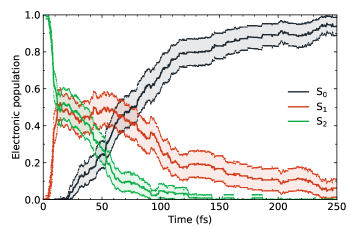
Figure 3: Electronic population evolution during TAB dynamics initiated in the S₂ state.

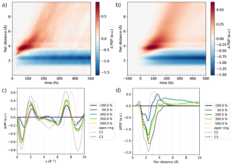
Figure 4: a) $\Delta$PDF simulated signal. b) Same signal convoluted with a 80 fs FWHM temporal Gaussian. c) Time slices of modified scattering intensity from $-100$ fs to 500 fs. Reference $\Delta sM$ signals for optimized C2 products, C3 products, and open ring structures in black. d) Time slices of $\Delta$PDF presented in the same manner.

The average adiabatic electronic populations predicted by our TAB simulations are displayed in Fig. 3. The lines represent the mean values over the ensemble of trajectories, and the shaded areas show the 95 % confidence interval based on the binomial distribution. (This confidence interval reflects only error associated with trajectory sampling, not error related to physical approximations.) Following excitation, the molecule undergoes rapid relaxation through a conical intersection (CI) to the S₁ state. Half of the original population transitions during the first 12 fs. However, it takes 65 fs until the S₂ population decays below 0.1. Next, the molecule resides in the S₁ state, from which it can continue to the ground state after reaching the respective CI. This requires crossing of a ring-opening transition state, which prolongs the relaxation time. After reaching the ground state, we observe the usual relaxation channels labeled as C2 for CH2CO + C2H4 products and C3 for C3H6 (cyclopropane) + CO products.

In addition to these main pathways, 19% of the population is observed to undergo ring-opening directly in the S₂ state, which contributes to the prolonged S₂ relaxation. The molecule then transitions to either S₁ or S₀ at various points in time. Both C2 and C3 channels are observed following relaxation to S₀. Within our sampling of 150 trajectories, it is not obvious that ring-opening on S₂ impacts the photoproduct distribution.

In total, most trajectories form the C3 products (60%), although the cyclization to cyclopropane is not always completed within our 1 ps simulation window. C2 products are created in 28% of cases. In the remaining 12% we observe some larger fragmentation of the original molecule or hydrogen dissociation.

From the TAB dynamics, we simulate the time-dependent $\Delta$PDF signal. Fig. 4 displays the resulting signal at simulation resolution (panel a) and convoluted by the experimental cross-correlation (panel b). There is a faint signal in the first tents of fs when the initial S${}_{2}\rightarrow$S₁ relaxation takes place. After that, we start to observe a new signal above the previously blank 3 $\mathrm{\SIUnitSymbolAngstrom}$ threshold. This is due to the ring-opening process and subsequent dissociation into distinct molecular products. Since the $\Delta$PDF fingerprints of individual intermediates and products are rather similar, it is difficult to discern between them using this plot. For easier analysis, we present time slices of the $\Delta$PDF data in Fig. 4d. The corresponding plot in momentum space—the difference modified scattering intensity ($\Delta sM$)—is shown in Fig. 4c. Reference signals associated with three static geometries are presented for comparison: a representative open ring intermediate structure and the C2 and C3 products. We have chosen the FOMO-CASCI-optimized S₁-S₀ minimal energy conical intersection structure (pictured in Fig. 2) to represent the ring-opened region of the PES. We do not mean to imply that signal in this region necessarily corresponds to detection of population at the conical intersection. However, it carries the ring-opening character which is specific for the product formation. The rest of the reference structures were optimized at B3LYP/6-311+G* level.

At 50 fs, both the $\Delta$PDF and difference modified scattering intensity ($\Delta sM$) exhibit features that are characteristic of the representative ring-opened (S₁-S₀ conical intersection) structure. In momentum space, the first negative peak (between 0 and 2 $\mathrm{\SIUnitSymbolAngstrom}$^-1) closely mirrors that of the ring-opened structure, and there is a pronounced negative peak at near 6 $\mathrm{\SIUnitSymbolAngstrom}$^-1 that does not appear in either the C2 or C3 products. In the $\Delta$PDF, there is a large positive peak just below 4 $\mathrm{\SIUnitSymbolAngstrom}$ that is characteristic of the ring-opened structure.

At later times, the signals evolve in a way that reflects the dissociation. In momentum space, the first negative peak intensifies and shifts to lower momentum (now below 1 $\mathrm{\SIUnitSymbolAngstrom}$^-1) upon dissociation. In position space, the large peak near 4 $\mathrm{\SIUnitSymbolAngstrom}$ loses intensity as the ring-opened structure dissociates. In addition, the broad negative feature between 1 and 3 $\mathrm{\SIUnitSymbolAngstrom}$ intensifies.

A detailed analysis of this broad negative feature allows discrimination between the C2 and C3 products. The lower-distance portion of this feature ($\sim$1.5 $\mathrm{\SIUnitSymbolAngstrom}$) corresponds to the loss of carbon-carbon bonds. The reactants contain four C-C bonds. The C3 products have three C-C bonds (all in cyclopropane), while the C2 product has only two (one in each product). Thus, as the ring-opened structure disappears, a more pronounced shoulder at $\sim$1.5 $\mathrm{\SIUnitSymbolAngstrom}$ is indicative of a lower C3/C2 branching ratio. Differences are also observed in the momentum-space representation. Between 4 and 5 $\mathrm{\SIUnitSymbolAngstrom}$^-1, both signals are negative, but the C2 products contribute a larger negative signal. Differences in the height and location of the first negative and positive peaks (near 0.5 and 2 $\mathrm{\SIUnitSymbolAngstrom}$^-1, respectively) are also observed when comparing the C2 and C3 products.

The presented results account for the first 500 fs of post-excitation dynamics, which could be reliably described using our limited number of trajectories. For longer times, we can expect slow decay of the dissociative signal (above 4 $\mathrm{\SIUnitSymbolAngstrom}$ in the $\Delta$PDF). Otherwise, the overall shape of the 500 fs time slices should remain relatively unchanged.

III.2 Discussion

The primary goal of the present work is to test our ability to predict an experimental measurement, a priori. However, it is worth discussing what kinds of errors we anticipate might arise from our approach before we have access to the result. Just as it is interesting to see if we can predict the experimental signal, it is interesting to see if we can predict which errors might manifest in that prediction. By recording our thinking, this prediction challenge will teach us not only about the accuracy of our methods, but also how well we understand them.

Let us first consider the reaction mechanism. A known advantage of ab initio molecular dynamics is that it allows us to simulate molecular dynamics with relatively little prior knowledge of the relevant reaction pathway(s) and without enduring a time- and resource-consuming PES fitting procedure. In the present case, we predict that the molecule undergoes ring-opening, followed by dissociation via the C2 and C3 channels. The final photochemical outcomes are not truly predictions, because they are known from past photochemical experiments,Denschlag and Lee (1968); Lee and Lee (2003); Lee (1977) but the initial ring opening step is a prediction, and would likely be observable in the experiment. Given that our simulations predict the initial and final states correctly, it seems likely that the prediction of the intermediate ring-opened intermediate state is correct as well. Thus, we expect this prediction to be robust.

Now, we consider the accuracy of our prediction of the experimental observable itself. As mentioned above, GUED is a powerful experiment in part because it can very accurately measure a time-dependent property (interatomic distance) that can also be very accurately predicted by simulation. We feel confident that the computed experimental observables ($\Delta$PDF and its momentum-space counterpart) are accurate.

Though we feel fairly confident about our predictions of mechanism and observable, our simulations also predict more challenging quantities: branching ratios and timescales. We expect these predictions to be challenging because the calculation of these properties involves the effective exponentiation of relative energies between points on the PES, via $\mathrm{e}^{-\Delta E/k_{\mathrm{B}}T}$ ($\Delta$E denoting relative energy, $k_{\rm{B}}$ the Boltzmann constant, and $T$ temperature). This exponentiation can amplify small errors in the PES into large errors in the property of interest. Our simulations are based on a relatively low level of electronic structure theory and some errors in the PES are inevitable. Therefore, predictions of rates and branching ratios are potentially less robust. A notable exception to this statement would be when the process of interest is governed by ballistic, rather than statistical, motion. The timescale of a ballistic process is governed by the gradient of the PES and the masses of the atoms. In such cases, there is no exponential amplification of error, and a robust prediction is more likely. In turn, we will consider potential errors in our predictions of the C3/C2 branching ratio, the timescale for $\rm{S}_{2}\rightarrow\rm{S}_{1}$ relaxation, and the timescale for subsequent $\rm{S}_{1}\rightarrow\rm{S}_{0}$ relaxation.

Both experiment and past theory suggest that the C3/C2 product ratio has a strong and complicated dependence on pump wavelength.Lee (1977); Denschlag and Lee (1968); Lee and Lee (2003) This behavior can be attributed to the nonequilibrium vibrational energy distribution driving the dynamics in short time.Liu and Fang (2016); Diau, Kötting, and Zewail (2001) Our simulations do not take the pump wavelength into account, except rather coarsely by the selection of our initial electronic state. Thus, we anticipate that error in our predicted branching ratio is a likely source of error in the predicted spectrum.

Next, we will consider the $\rm{S}_{2}\rightarrow\rm{S}_{1}$ relaxation process. To this end, we can estimate the excited state lifetime from existing spectroscopic data.Udvarhazi and El-Sayed (2004); Hemminger, Carless, and Lee (1973) Heller describes the relation between decay times of the wavepacket’s autocorrelation function and the width of absorption spectrum peaks.Heller (1981) Since there is a clear vibronic resolution of the first Rydberg state, we can infer the expected state’s half-life in this way. The full width at the half maximum (FWHM) of a single subpeak can be estimated to around 0.02 eV. We can infer the state’s half-life by taking the reciprocal of FWHM, yielding 34 fs. Though the decay of S₂ is non-exponential in our simulations, the simulated dynamics are consistent with the inferred experimental timescale; the S₂ population decays to 0.5 in the first 12 fs, and then to 0.25 by $\sim$50 fs. Given that this relaxation occurs in the first 1–3 vibrational periods, it appears to be a ballistic, barrierless process; thus it is not surprising that our predication here appears robust.

Finally, we consider the $\rm{S}_{1}\rightarrow\rm{S}_{0}$ relaxation process. In the case of cyclobutanone the height of the S₁ transition state and the available vibrational energy will determine the overall kinetics of the process. To estimate possible errors in our S₁ decay rate, we assume the rate-limiting step is traversing the S₁ transition state and apply Rice–Ramsperger–Kassel–Marcus (RRKM) theoryMarcus (2004) to predict the lifetime on a more accurate PES as a function of excess pump energy. RRKM assumes the internal energy is randomly distributed among the vibrational modes of the molecule, and the reaction occurs when enough energy accumulates in the reactive mode. The rate constant is evaluated using the formula

$$k(E)=\frac{\sigma W^{{\ddagger}}(E-E_{0})}{h\rho(E)},$$ (11)

where $W^{{\ddagger}}$ denotes the number of accessible vibrational states of the transition state (S₁TS), excluding those leading to the reaction, and $\rho$ the density of states of the reactant (S₁min). The available internal energy of the system is $E$, and $E_{0}$ is the barrier height, both relative to the S₁ minimum in our case. Planck’s constant is $h$, and $\sigma$ represents degeneracy of the reaction pathway. We set $\sigma$ to 2, since there are two symmetry-equivalent ring-opening reactions. Here, we use previously optimized structures from ref. 80, recalculating the energies and frequencies with the highly accurate complete active space second-order perturbation theory (CASPT2) method. We choose an active space of 10 electrons in 8 orbitals (CASPT2(10,8)) and the 6-31G* basis. Zero-point energy is included. To calculate the number of states, we use the Beyer-Swinehart algorithm.Beyer and Swinehart (1973)

To calibrate our surface, we first estimate the half-life upon excitation at 281 nm (4.41 eV) and 255 nm (4.85 eV), which correspond to transient absorption measurements by Kao, et al.Kao et al. (2020) The computed half-lives (1160 and 400 fs at 281 and 255 nm, respectively) are within a factor of three of the shortest experimental timescale (450 fs, which was determined in a global fit including both experiments at 281 nm and 255 nmKao et al. (2020)). Given that one would expect a fairly strong wavelength dependence for this rate that is not discerned by the global experimental fit, it is difficult to say anything more specific than that RRKM/CASPT2 provides a reasonable estimate of the lifetime.

Now we consider the current simulations. We assume that all excess energy in the 200 nm (6.2 eV) pump pulse is thermalized on S₁ prior to the reaction. Within these assumptions, RRKM predicts an S₁ state half-life of 120 fs, which is longer than our simulated timescale by a factor of 2. One can attribute this discrepancy to two different factors: FOMO-CASCI may predict a barrier on S₁ that is too small, and/or the assumption of thermalization on S₁ in RRKM may be invalid here. If all error is attributable to the assumption of thermalization, we would anticipate very little error in our predicted lifetime. However, if the error is attributed to the FOMO-CASCI barrier height, it is imaginable that we underestimate the timescale for the $\rm{S}_{1}\rightarrow\rm{S}_{0}$ relaxation by a factor of 2, or even more. Keeping in mind that the timescales are exponentially sensitive to errors in the PES, this degree of uncertainty is not surprising. With additional time and computational effort, simulations based on CASPT2 or another highly accurate ab initio method would allow a more definitive prediction of the timescale.

IV Conclusions

Above, we report a prediction of the GUED spectrum of cyclobutanone, excited to the 3s Rydberg state, for comparison to an upcoming experiment. To this end, we applied an ab initio molecular dynamics approach based on the TAB nonadiabatic mixed quantum-classical method to simulate the dynamics following the initial pump pulse, and then we directly simulated the experimental observable. Our simulations show two distinct dissociation pathways that share a common ring-opened intermediate. Analysis of the predicted GUED signal provides guidance on how the ring-opened intermediate, C2 products, and C3 products can be discerned in the spectrum.

We also present our own a priori assessment of the most likely sources of error in our prediction. Although the details are specific to our group’s prediction, the general conclusions of our analysis apply broadly to all prediction attempts; the two most likely modes of failure for this prediction challenge are a) an incorrect prediction of the branching ratio between the C2 and C3 channels, and b) an incorrect prediction of the lifetime for barrier crossing on S₁. This is because these two processes are governed by statistical motion, and therefore small errors in relative energies will be amplified via the Boltzmann factor $\mathrm{e}^{-\Delta E/k_{\mathrm{B}}T}$ into large errors in the quantity of interest. Ultimately, these errors arise from the approximate electronic structure methods used in dynamic simulations, more so than the chosen dynamical method.

Importantly, robust predictions of mechanisms and their observable signatures are likely to be sufficient to definitively assign the experimental spectrum, even in the case that predicted lifetimes and branching ratios have significant errors. Thus, even a simulation that fails as a standalone prediction may provide essential insight into the dynamics of cyclobutanone when interpreted in the context of the experimental data.

Author declarations

Conflict of interest

The authors have no conflicts to disclose.

Author Contributions

Jiří Suchan: Investigation (lead); Software (supporting); Writing – original draft (equal); Writing – review & editing (equal). Fangchun Liang: Software (equal). Andrew S. Durden: Software (equal). Benjamin G. Levine: Writing – original draft (equal); Writing – review & editing (equal).

Data Availability Statement

Data available on request from the authors.

References

- Zewail (2000) A. Zewail, The Journal of Physical Chemistry A 104, 5660 (2000).
- Schwartz and Rossky (1994) B. J. Schwartz and P. J. Rossky, The Journal of Physical Chemistry 98, 4489 (1994).
- Batista and Coker (1997) V. S. Batista and D. F. Coker, The Journal of Chemical Physics 106, 6923 (1997).
- Vreven et al. (1997) T. Vreven, F. Bernardi, M. Garavelli, M. Olivucci, M. Robb, and H. Schlegel, Journal of the American Chemical Society 119, 12687 (1997).
- Ben-Nun and Martinez (1998) M. Ben-Nun and T. Martinez, Chemical Physics Letters 298, 57 (1998).
- Subotnik et al. (2016) J. E. Subotnik, A. Jain, B. Landry, A. Petit, W. Ouyang, and N. Bellonzi, Annual Review of Physical Chemistry 67, 387 (2016), pMID: 27215818, https://doi.org/10.1146/annurev-physchem-040215-112245 .
- Crespo-Otero and Barbatti (2018) R. Crespo-Otero and M. Barbatti, Chemical Reviews 118, 7026 (2018), pMID: 29767966, https://doi.org/10.1021/acs.chemrev.7b00577 .
- Curchod and Martínez (2018) B. F. E. Curchod and T. J. Martínez, Chemical Reviews 118, 3305 (2018), pMID: 29465231, https://doi.org/10.1021/acs.chemrev.7b00423 .
- Gonzalez and Lindh (2021) L. Gonzalez and R. Lindh, Quantum chemistry and dynamics of excited states : methods and applications (John Wiley & Sons, Ltd, Hoboken, NJ, 2021).
- Agostini and Gross (2021) F. Agostini and E. K. U. Gross, European Physical Journal B 94 (2021), 10.1140/epjb/s10051-021-00171-2.
- Ibele and Curchod (2020) L. M. Ibele and B. F. E. Curchod, Physical Chemistry Chemical Physics 22, 15183 (2020).
- Janos and Slavicek (2023) J. Janos and P. Slavicek, Journal of Chemical Theory and Computation 19, 8273 (2023).
- Akimov (2016) A. V. Akimov, Journal of Computational Chemistry 37, 1626 (2016).
- Mai, Marquetand, and Gonzalez (2018) S. Mai, P. Marquetand, and L. Gonzalez, Wiley Interdisciplinary Reviews: Computational Molecular Science 8 (2018), 10.1002/wcms.1370.
- Fedorov et al. (2020) D. A. Fedorov, S. Seritan, B. S. Fales, T. J. Martinez, and B. G. Levine, Journal of Chemical Theory and Computation 16, 5485 (2020).
- Malone et al. (2020) W. Malone, B. Nebgen, A. White, Y. Zhang, H. Song, J. A. Bjorgaard, A. E. Sifain, B. Rodriguez-Hernandez, V. M. Freixas, S. Fernandez-Alberti, A. E. Roitberg, T. R. Nelson, and S. Tretiak, Journal of Chemical Theory and Computation 16, 5771 (2020).
- Barbatti et al. (2022) M. Barbatti, M. Bondanza, R. Crespo-Otero, B. Demoulin, P. O. Dral, G. Granucci, F. Kossoski, H. Lischka, B. Mennucci, S. Mukherjee, M. Pederzoli, M. Persico, M. Pinheiro, J. Pittner, F. Plasser, E. S. Gil, and L. Stojanovic, Journal of Chemical Theory and Computation 18, 6851 (2022).
- Richter et al. (2012) M. Richter, P. Marquetand, J. Gonzalez-Vazquez, I. Sola, and L. Gonzalez, The Journal of Physical Chemistry Letters 3, 3090 (2012).
- Penfold et al. (2012) T. J. Penfold, R. Spesyvtsev, O. M. Kirkby, R. S. Minns, D. S. N. Parker, H. H. Fielding, and G. A. Worth, The Journal of Chemical Physics 137 (2012), 10.1063/1.4767054.
- Nelson et al. (2014) T. Nelson, S. Fernandez-Alberti, A. E. Roitberg, and S. Tretiak, Accounts of Chemical Research 47, 1155 (2014).
- Tavernelli (2015) I. Tavernelli, Accounts of Chemical Research 48, 792 (2015).
- Wang, Long, and Prezhdo (2015) L. Wang, R. Long, and O. V. Prezhdo, Annual Review of Physical Chemistry 66, 549 (2015), pMID: 25622188, https://doi.org/10.1146/annurev-physchem-040214-121359 .
- Fielding and Worth (2018) H. H. Fielding and G. A. Worth, Chemical Society Reviews 47, 309 (2018).
- Schuurman and Stolow (2018) M. S. Schuurman and A. Stolow, Annual Review of Physical Chemistry 69, 427 (2018), pMID: 29490199, https://doi.org/10.1146/annurev-physchem-052516-050721 .
- Popp et al. (2021) W. Popp, D. Brey, R. Binder, and I. Burghardt, Annual Review of Physical Chemistry 72, 591 (2021), pMID: 33636997.
- Talotta, Lauvergnat, and Agostini (2022) F. Talotta, D. Lauvergnat, and F. Agostini, The Journal of Chemical Physics 156 (2022), 10.1063/5.0089415.
- Dergachev et al. (2023) I. D. Dergachev, V. D. Dergachev, M. Rooein, A. Mirzanejad, and S. A. Varganov, Accounts of Chemical Research 56, 856 (2023).
- Hudock et al. (2007) H. R. Hudock, B. G. Levine, A. L. Thompson, H. Satzger, D. Townsend, N. Gador, S. Ullrich, A. Stolow, and T. J. Martínez, The Journal of Physical Chemistry A 111, 8500 (2007), pMID: 17685594, https://doi.org/10.1021/jp0723665 .
- Mitric et al. (2011) R. Mitric, J. Petersen, M. Wohlgemuth, U. Werner, V. Bonacic-Koutecky, L. Woeste, and J. Jortner, The Journal of Physical Chemistry A 115, 3755 (2011).
- De Giovannini et al. (2013) U. De Giovannini, G. Brunetto, A. Castro, J. Walkenhorst, and A. Rubio, ChemPhysChem 14, 1363 (2013).
- Petit and Subotnik (2014) A. S. Petit and J. E. Subotnik, The Journal of Chemical Physics 141, 154108 (2014).
- Fischer, Cramer, and Govind (2015) S. A. Fischer, C. J. Cramer, and N. Govind, Journal of Chemical Theory and Computation 11, 4294 (2015).
- Nguyen et al. (2016) T. S. Nguyen, J. H. Koh, S. Lefelhocz, and J. Parkhill, The Journal of Physical Chemistry Letters 7, 1590 (2016).
- Dsouza et al. (2018) R. Dsouza, X. Cheng, Z. Li, R. J. D. Miller, and M. A. Kochman, The Journal of Physical Chemistry A 122, 9688 (2018).
- Bonafé et al. (2018) F. P. Bonafé, F. J. Hernández, B. Aradi, T. Frauenheim, and C. G. Sánchez, The Journal of Physical Chemistry Letters 9, 4355 (2018).
- Gelin et al. (2021) M. F. Gelin, X. Huang, W. Xie, L. Chen, N. Došlić, and W. Domcke, Journal of Chemical Theory and Computation 17, 2394 (2021).
- Kochman, Durbeej, and Kubas (2021) M. A. Kochman, B. Durbeej, and A. Kubas, The Journal of Physical Chemistry A 125, 8635 (2021).
- Borrego-Varillas et al. (2021) R. Borrego-Varillas, A. Nenov, P. Kabaciński, I. Conti, L. Ganzer, A. Oriana, V. K. Jaiswal, I. Delfino, O. Weingart, C. Manzoni, I. Rivalta, M. Garavelli, and G. Cerullo, Nature Communications 12, 7285 (2021).
- Xu et al. (2022) C. Xu, K. Lin, D. Hu, F. L. Gu, M. F. Gelin, and Z. Lan, The Journal of Physical Chemistry Letters 13, 661 (2022), https://doi.org/10.1021/acs.jpclett.1c03373 .
- Chakraborty et al. (2022) P. Chakraborty, Y. Liu, S. McClung, T. Weinacht, and S. Matsika, The Journal of Physical Chemistry A (2022), 10.1021/acs.jpca.2c04671.
- Silfies et al. (2023) M. C. Silfies, A. Mehmood, G. Kowzan, E. G. Hohenstein, B. G. Levine, and T. K. Allison, The Journal of Chemical Physics 159 (2023), 10.1063/5.0161238.
- Young et al. (2018) L. Young, K. Ueda, M. Gühr, P. H. Bucksbaum, M. Simon, S. Mukamel, N. Rohringer, K. C. Prince, C. Masciovecchio, M. Meyer, et al., Journal of Physics B: Atomic, Molecular and Optical Physics 51, 032003 (2018).
- Nisoli et al. (2017) M. Nisoli, P. Decleva, F. Calegari, A. Palacios, and F. Martín, Chemical reviews 117, 10760 (2017).
- Kowalewski et al. (2017) M. Kowalewski, B. P. Fingerhut, K. E. Dorfman, K. Bennett, and S. Mukamel, Chemical Reviews 117, 12165 (2017).
- Neville et al. (2018) S. P. Neville, M. Chergui, A. Stolow, and M. S. Schuurman, Physical review letters 120 (2018), 10.1103/PhysRevLett.120.243001.
- Li et al. (2020) X. Li, N. Govind, C. Isborn, A. E. I. DePrince, and K. Lopata, Chemical Reviews 120, 9951 (2020), pMID: 32813506, https://doi.org/10.1021/acs.chemrev.0c00223 .
- Zinchenko et al. (2021) K. S. Zinchenko, F. Ardana-Lamas, I. Seidu, S. P. Neville, J. van der Veen, V. U. Lanfaloni, M. S. Schuurman, and H. J. Worner, Science 371, 489+ (2021).
- Freixas et al. (2022) V. M. Freixas, D. Keefer, S. Tretiak, S. Fernandez-Alberti, and S. Mukamel, Chemical Science 13, 6373 (2022).
- Centurion, Wolf, and Yang (2022) M. Centurion, T. J. Wolf, and J. Yang, Annual Review of Physical Chemistry 73, 21 (2022), pMID: 34724395, https://doi.org/10.1146/annurev-physchem-082720-010539 .
- Williamson et al. (1997) J. Williamson, J. Cao, H. Ihee, H. Frey, and A. Zewail, NATURE 386, 159 (1997).
- Ihee et al. (2001) H. Ihee, V. Lobastov, U. Gomez, B. Goodson, R. Srinivasan, C. Ruan, and A. Zewail, Science 291, 458 (2001).
- Yang et al. (2016a) J. Yang, M. Guehr, T. Vecchione, M. S. Robinson, R. Li, N. Hartmann, X. Shen, R. Coffee, J. Corbett, A. Fry, K. Gaffney, T. Gorkhover, C. Hast, K. Jobe, I. Makasyuk, A. Reid, J. Robinson, S. Vetter, F. Wang, S. Weathersby, C. Yoneda, M. Centurion, and X. Wang, Nature Communications 7 (2016a), 10.1038/ncomms11232.
- Yang et al. (2016b) J. Yang, M. Guehr, X. Shen, R. Li, T. Vecchione, R. Coffee, J. Corbett, A. Fry, N. Hartmann, C. Hast, K. Hegazy, K. Jobe, I. Makasyuk, J. Robinson, M. S. Robinson, S. Vetter, S. Weathersby, C. Yoneda, X. Wang, and M. Centurion, Physical review letters 117 (2016b), 10.1103/PhysRevLett.117.153002.
- Yang et al. (2018) J. Yang, X. Zhu, T. J. A. Wolf, Z. Li, J. P. F. Nunes, R. Coffee, J. P. Cryan, M. Guehr, K. Hegazy, T. F. Heinz, K. Jobe, R. Li, X. Shen, T. Veccione, S. Weathersby, K. J. Wilkin, C. Yoneda, Q. Zheng, T. J. Martinez, M. Centurion, and X. Wang, Science 361, 64 (2018).
- Wolf et al. (2019) T. J. A. Wolf, D. M. Sanchez, J. Yang, R. M. Parrish, J. P. F. Nunes, M. Centurion, R. Coffee, J. P. Cryan, M. Guehr, K. Hegazy, A. Kirrander, R. K. Li, J. Ruddock, X. Shen, T. Vecchione, S. P. Weathersby, P. M. Weber, K. Wilkin, H. Yong, Q. Zheng, X. J. Wang, M. P. Minitti, and T. J. Martinez, Nature chemistry 11, 504 (2019).
- Stefanou et al. (2017) M. Stefanou, K. Saita, D. V. Shalashilin, and A. Kirrander, Chemical Physics Letters 683, 300 (2017), ahmed Zewail (1946-2016) Commemoration Issue of Chemical Physics Letters.
- Parrish and Martínez (2019) R. M. Parrish and T. J. Martínez, Journal of Chemical Theory and Computation 15, 1523 (2019), pMID: 30702882, https://doi.org/10.1021/acs.jctc.8b01051 .
- Champenois et al. (2021) E. G. Champenois, D. M. Sanchez, J. Yang, J. P. F. Nunes, A. Attar, M. Centurion, R. Forbes, M. Gühr, K. Hegazy, F. Ji, S. K. Saha, Y. Liu, M.-F. Lin, D. Luo, B. Moore, X. Shen, M. R. Ware, X. J. Wang, T. J. Martínez, and T. J. A. Wolf, Science 374, 178 (2021), https://www.science.org/doi/pdf/10.1126/science.abk3132 .
- Liu et al. (2023) Y. Liu, D. M. Sanchez, M. R. Ware, E. G. Champenois, J. Yang, J. P. F. Nunes, A. Attar, M. Centurion, J. P. Cryan, R. Forbes, et al., Nature Communications 14, 2795 (2023).
- Weathersby et al. (2015) S. P. Weathersby, G. Brown, M. Centurion, T. F. Chase, R. Coffee, J. Corbett, J. P. Eichner, J. C. Frisch, A. R. Fry, M. Gühr, N. Hartmann, C. Hast, R. Hettel, R. K. Jobe, E. N. Jongewaard, J. R. Lewandowski, R. K. Li, A. M. Lindenberg, I. Makasyuk, J. E. May, D. McCormick, M. N. Nguyen, A. H. Reid, X. Shen, K. Sokolowski-Tinten, T. Vecchione, S. L. Vetter, J. Wu, J. Yang, H. A. Dürr, and X. J. Wang, Review of Scientific Instruments 86, 073702 (2015), https://pubs.aip.org/aip/rsi/article-pdf/doi/10.1063/1.4926994/15949942/073702_1_online.pdf .
- Note (1) We submitted this work to arxiv on Jan. 15, 2024. DOI:XXXXX.
- Esch and Levine (2020a) M. P. Esch and B. G. Levine, The Journal of Chemical Physics 152 (2020a), 10.1063/5.0010081.
- Esch and Levine (2021) M. P. Esch and B. Levine, The Journal of Chemical Physics 155, 214101 (2021), https://pubs.aip.org/aip/jcp/article-pdf/doi/10.1063/5.0070686/14878146/214101_1_online.pdf .
- Durden et al. (2024) A. S. Durden, F. Liang, J. Suchan, A. Teplukhin, and B. G. Levine, (2024), 10.5281/zenodo.10498050.
- Tully (1990) J. C. Tully, The Journal of Chemical Physics 93, 1061 (1990), https://pubs.aip.org/aip/jcp/article-pdf/93/2/1061/11035518/1061_1_online.pdf .
- Bittner and Rossky (1995) E. R. Bittner and P. J. Rossky, The Journal of Chemical Physics 103, 8130 (1995), https://pubs.aip.org/aip/jcp/article-pdf/103/18/8130/10778767/8130_1_online.pdf .
- Schwartz et al. (1996) B. J. Schwartz, E. R. Bittner, O. V. Prezhdo, and P. J. Rossky, The Journal of Chemical Physics 104, 5942 (1996), https://pubs.aip.org/aip/jcp/article-pdf/104/15/5942/8105629/5942_1_online.pdf .
- Esch, Shu, and Levine (2019) M. P. Esch, Y. Shu, and B. G. Levine, The Journal of Physical Chemistry A 123, 2661 (2019).
- Esch and Levine (2020b) M. P. Esch and B. G. Levine, The Journal of Chemical Physics 153 (2020b), 10.1063/5.0022529.
- Peng, Fales, and Levine (2018) W.-T. Peng, B. S. Fales, and B. G. Levine, Journal of Chemical Theory and Computation 14, 4129 (2018), pMID: 29986143, https://doi.org/10.1021/acs.jctc.8b00381 .
- Durden and Levine (2022) A. S. Durden and B. G. Levine, Journal of Chemical Theory and Computation 18, 795 (2022).
- Gray and Manolopoulos (1996) S. Gray and D. Manolopoulos, The Journal of Chemical Physics 104, 7099 (1996).
- Seritan et al. (2021) S. Seritan, C. Bannwarth, B. S. Fales, E. G. Hohenstein, C. M. Isborn, S. I. L. Kokkila-Schumacher, X. Li, F. Liu, N. Luehr, J. W. Snyder Jr., C. Song, A. V. Titov, I. S. Ufimtsev, L.-P. Wang, and T. J. Martínez, WIREs Computational Molecular Science 11, e1494 (2021), https://wires.onlinelibrary.wiley.com/doi/pdf/10.1002/wcms.1494 .
- Ufimtsev and Martinez (2008) I. S. Ufimtsev and T. J. Martinez, Journal of Chemical Theory and Computation 4, 222 (2008).
- Ufimtsev and Martinez (2009a) I. S. Ufimtsev and T. J. Martinez, Journal of Chemical Theory and Computation 5, 1004 (2009a).
- Ufimtsev and Martinez (2009b) I. S. Ufimtsev and T. J. Martinez, Journal of Chemical Theory and Computation 5, 2619 (2009b).
- Fales and Levine (2015) B. S. Fales and B. G. Levine, Journal of Chemical Theory and Computation 11, 4708 (2015).
- Hohenstein et al. (2015) E. G. Hohenstein, M. E. F. Bouduban, C. Song, N. Luehr, I. S. Ufimtsev, and T. J. Martinez, The Journal of Chemical Physics 143 (2015), 10.1063/1.4923259.
- Liu and Fang (2016) L. Liu and W.-H. Fang, The Journal of Chemical Physics 144, 144317 (2016), https://pubs.aip.org/aip/jcp/article-pdf/doi/10.1063/1.4945782/13555376/144317_1_online.pdf .
- Xia et al. (2015) S.-H. Xia, X.-Y. Liu, Q. Fang, and G. Cui, The Journal of Physical Chemistry A 119, 3569 (2015), pMID: 25807113, https://doi.org/10.1021/acs.jpca.5b00302 .
- Diau, Kötting, and Zewail (2001) E. W.-G. Diau, C. Kötting, and A. H. Zewail, ChemPhysChem 2, 294 (2001).
- Hemminger and Lee (2003) J. C. Hemminger and E. K. C. Lee, The Journal of Chemical Physics 56, 5284 (2003), https://pubs.aip.org/aip/jcp/article-pdf/56/11/5284/11101722/5284_1_online.pdf .
- Udvarhazi and El-Sayed (2004) A. Udvarhazi and M. A. El-Sayed, The Journal of Chemical Physics 42, 3335 (2004), https://pubs.aip.org/aip/jcp/article-pdf/42/9/3335/11206722/3335_1_online.pdf .
- Hemminger, Carless, and Lee (1973) J. Hemminger, H. A. Carless, and E. K. Lee, Journal of the American Chemical Society 95, 682 (1973).
- Levine et al. (2021) B. G. Levine, A. S. Durden, M. P. Esch, F. Liang, and Y. Shu, The Journal of Chemical Physics 154, 090902 (2021), https://doi.org/10.1063/5.0042147 .
- Slavíček and Martínez (2010) P. Slavíček and T. J. Martínez, The Journal of Chemical Physics 132, 234102 (2010), https://pubs.aip.org/aip/jcp/article-pdf/doi/10.1063/1.3436501/16031951/234102_1_online.pdf .
- Granucci, Persico, and Toniolo (2001) G. Granucci, M. Persico, and A. Toniolo, The Journal of Chemical Physics 114, 10608 (2001).
- Salvat, Jablonski, and Powell (2005) F. Salvat, A. Jablonski, and C. J. Powell, Computer Physics Communications 165, 157 (2005).
- Denschlag and Lee (1968) H. Denschlag and E. K. Lee, Journal of the American Chemical Society 90, 3628 (1968).
- Lee and Lee (2003) N. E. Lee and E. K. C. Lee, The Journal of Chemical Physics 50, 2094 (2003), https://pubs.aip.org/aip/jcp/article-pdf/50/5/2094/11098793/2094_1_online.pdf .
- Lee (1977) E. K. C. Lee, Accounts of Chemical Research 10, 319 (1977), https://doi.org/10.1021/ar50117a002 .
- Heller (1981) E. J. Heller, Accounts of Chemical Research 14, 368 (1981).
- Marcus (2004) R. A. Marcus, The Journal of Chemical Physics 20, 359 (2004), https://pubs.aip.org/aip/jcp/article-pdf/20/3/359/8113340/359_1_online.pdf .
- Beyer and Swinehart (1973) T. Beyer and D. F. Swinehart, 16 (1973), 10.1145/362248.362275.
- Kao et al. (2020) M.-H. Kao, R. K. Venkatraman, M. N. R. Ashfold, and A. J. Orr-Ewing, Chem. Sci. 11, 1991 (2020).
- O’Toole et al. (1991) L. O’Toole, P. Brint, C. Kosmidis, G. Boulakis, and P. Tsekeris, J. Chem. Soc., Faraday Trans. 87, 3343 (1991).
- Thompson, Punwong, and Martínez (2010) A. L. Thompson, C. Punwong, and T. J. Martínez, Chemical Physics 370, 70 (2010), dynamics of molecular systems: From quantum to classical.
- Richings and Habershon (2022) G. W. Richings and S. Habershon, Accounts of Chemical Research 55, 209 (2022).
- Worth and Cederbaum (2004) G. Worth and L. Cederbaum, Annual Review of Physical Chemistry 55, 127 (2004).
- Liu et al. (2020) Y. Liu, S. L. Horton, J. Yang, J. P. F. Nunes, X. Shen, T. J. A. Wolfe, R. Forbes, C. Cheng, B. Moore, M. Centurion, K. Hegazy, R. Li, M.-F. Lin, A. Stolow, P. Hockett, T. Rozgonyi, P. Marquetand, X. Wang, and T. Weinacht, Physical Review X 10 (2020), 10.1103/PhysRevX.10.021016.