Strong Bayesian Evidence for the
Normal Neutrino Hierarchy
Abstract
The configuration of the three neutrino masses can take two forms, known as the normal and inverted hierarchies. We compute the Bayesian evidence associated with these two hierarchies. Previous studies found a mild preference for the normal hierarchy, and this was driven by the asymmetric manner in which cosmological data has confined the available parameter space. Here we identify the presence of a second asymmetry, which is imposed by data from neutrino oscillations. By combining constraints on the squared-mass splittings [2] with the limit on the sum of neutrino masses of eV [3], and using a minimally informative prior on the masses, we infer odds of 42:1 in favour of the normal hierarchy, which is classified as “strong” in the Jeffreys’ scale. We explore how these odds may evolve in light of higher precision cosmological data, and discuss the implications of this finding with regards to the nature of neutrinos. Finally the individual masses are inferred to be ( credible intervals).
1 Introduction
Cosmological surveys provide crucial information on the absolute masses of neutrinos, information that is not accessible even to future laboratory experiments [4, 5, 6]. Recent analyses have already established a robust upper limit on the sum of neutrino masses of eV [3] and [7] at 95% confidence (throughout this work we shall denote as for brevity). This limit is tantalisingly close to the lower limit for the sum of the masses in the inverted hierarchy eV (68% C.L.) [2]. Because the volume covered by cosmological surveys keeps increasing, their statistical errors shrink, soon leading to either (a) a measure the total neutrino mass or (b) the exclusion of the inverted hierarchy, leaving the normal one as the only viable option. It is therefore possible to determine the neutrino hierarchy, even in the absence of a measurement of the total mass e.g., Ref. [8, 9, 10]. Future surveys may even yield a measurement of the mass differences between the lightest and heaviest eigenstates [11]. This measurement would also provide a powerful consistency check: the measured mass splitting from cosmology should be consistent with the squared mass splitting from oscillations. Given the current knowledge about mass splitting and cosmological constraints on the total mass, can anything be said about the neutrino mass hierarchy?
Since current cosmological upper limits are already close to the inverted hierarchy bound, the volume of parameter space available is heavily restricted. As such, it is useful to employ Bayesian evidence methods in order to determine which hierarchy is favoured by the data. While it seems counterintuitive that one can determine a quantity without having actually measured it, consider the following pedagogical example: if there is a thin stick of length hidden underneath a cloth, one does not necessarily need to reveal the object in order to learn of its orientation. At the start, it is considered equally likely to be in either a horizontal or vertical position. If the cloth is gradually withdrawn in the horizontal direction, and no sign of the stick emerges, one need not wait until a residual length less than is left unexposed to be confident of a vertical orientation. Even while a full of the surface remains covered, the odds are already stacked in favour of a vertical orientation.
Our main objective is to identify which hierarchy is preferred by the Bayesian evidence ratio, and understand how this is likely to evolve as new cosmological data arrives in the near future. Previous inferences on the neutrino hierarchy have been made by e.g., Refs. [12, 13, 14]. One crucial aspect where our work differs from previous work in the literature is the choice and the dimensionality of the prior, which we shall explore in detail. We will also outline the consequences and implications of identifying the nature of the neutrino hierarchy.
2 Cosmology, oscillations, and statistics
In this section we provide a brief review of the three disciplines that are central to this work.
2.1 Cosmology: observational constraints and degeneracies
Massive neutrinos influence both the expansion history and growth of structure in the Universe. Neutrinos of mass eV become non-relativistic after the epoch of recombination probed by the Cosmic Microwave Background (CMB), and this mechanism allows massive neutrinos to alter the relationship connecting the physical matter density to the redshift of matter-radiation equality. The neutrinos’ radiation-like behaviour at early times modulates the peak positions in the CMB angular power spectrum. However this effect is somewhat degenerate with other cosmological parameters. Neutrinos are also responsible for dampening the matter power spectrum below their free-streaming scale; see e.g., [15] for a review. This effect, which amounts to a scale dependent power suppression, is straightforward to compute in linear theory [16] and in the non-linear regime via numerical simulations e.g., [17, 18, 19].
Due to these mechanisms, cosmological observables are predominantly sensitive to the sum of neutrino masses e.g., [20, 21, 22, 15, 23, 24, 25]. While the effect of neutrino mass on the CMB is related to the physical density of neutrinos, and therefore the mass difference between eigenstates can be neglected, individual neutrino masses, however, can have an effect on the large-scale shape of the matter power spectrum. Neutrinos of different masses have different transition redshifts from relativistic to non-relativistic behaviour, and their mass splitting changes the details of the radiation-domination to matter-domination regime. A precise measurement of the matter power spectrum shape can give information on both the sum of the masses and individual masses (and thus the hierarchy), even if the second effect is much smaller than the first [11].
In this work we shall utilise cosmological constraints imposed on the sum of the three neutrino masses, . The notation we shall use to denote the three neutrino mass eigenstates is , , and . Thus there are only two independent neutrino mass squared differences. In this convention and refer to the smaller square mass difference. Thus there are two possible hierarchies only. In what is known as the normal mass hierarchy, , , and are defined in ascending order, . For the case of the inverted hierarchy, the sequence becomes . In other words the hierarchy does not strictly corresponds to whether we have two small masses and one large or vice versa, this arises only once the results of the measurements of atmospheric and solar oscillations square mass splitting are in hand; the hierarchy is given by the sign of the square mass splitting involving .
Significant progress has been made by cosmological surveys to constrain the total mass of neutrinos. For example, the latest Planck satellite results show that CMB data alone constrain eV (95% C.L.) [26], where the upper limit is stronger than eV because of the extra constraining power offered by secondary effects, mostly lensing. The inclusion of late-time information about the cosmic expansion history, such as that provided by measurements of the Baryon Acoustic Oscillations (BAO), further breaks cosmological parameters degeneracies yielding a limit eV (95% C.L.).
Including information about the shape of the matter power spectrum further tightens these constraints, even when BAO information is not used. In Ref. [3] the authors have carefully examined the impact of using different galaxy populations and tracers to estimate the power spectrum of the underlying dark matter and concluded that eV at 95% confidence. This constraint tightens to eV if also the latest measurement of the Hubble constant [27] are included. Ref. [3] result is consistent with the previous constraint from a different estimate of the power spectrum of dark matter using the Lyman- forest [7], eV (see also [28, 29]). Since all these measurements are only upper limits for which the maxima of the probability distributions are indistinguishable from zero, unless otherwise stated, we will assume that the probability distributions for obtained from cosmological data are peaked at .
All the above constraints assume a standard cosmological model, where the spatial geometry is flat, dark matter (excluding the neutrino component) is cold, the dark energy is a cosmological constant, general relativity is the correct description of gravity on large, cosmological scales, the initial conditions of the Universe are given by a process like inflation and thus the primordial power spectrum is a nearly scale invariant power law. In addition, it is implicitly assumed that modelling of real world effects such as tracer’s bias, non-linearities, etc. is sufficiently accurate as not to induce systematic errors that are larger than the reported ones. Relaxing any of these assumptions would weaken the constraints significantly e.g., [30, 31, 32].
2.2 Neutrino Experiments
Solar, atmospheric, reactor and accelerator neutrino experiments have observed neutrino flavor conversion driven by neutrino masses. The experiments that mostly contribute to a precise measurement of the neutrino masses are sensitive to the relative phases acquired by relativistic neutrinos on their way from the production zone to the detector. Therefore the neutrino oscillation observables are sensitive to mass splittings, specifically to differences in the square of their masses. Matter effects allow the sign of the mass splittings to be distinguished, a goal which has been achieved in the small mass squared splitting but not the large one. The degeneracy in this second case distinguishes the two hierarchy mass orderings, normal and inverted. Identifying the neutrino mass hierarchy is a key objective for future neutrino oscillation experiments, in addition to a determination of the complex phase involved in flavor conversion.
The absolute neutrino mass is not accessible via flavor conversion experiments, but it can be probed using beta decay. Experiments require sufficient mass and very good energy resolution in order to measure the beta spectrum close to the endpoint, where the neutrino energy is the neutrino mass. The experiments measure the effective mass of the electron, which is the combination of neutrino masses weighted by their content in the electron flavor. The present bound derived from the electron mass is 2.3 eV (eV) at 90% confidence. The KATRIN experiment is expected to significantly improve upon this bound, reaching approximately 0.2 eV (eV) at 90% [4]. Meanwhile new proposals [5] like Project 8 [6] aim for yet greater sensitivity.
2.3 Bayesian Model Selection
In this work we shall employ Bayesian model selection in order to quantify the manner in which the combination of existing data, from both cosmology and neutrino experiments, should influence our belief in the normal or inverted hierarchy. Each hypothesis possesses the same number of free parameters, facilitating a fair comparison between the two. Furthermore their low dimensionality (three masses) permits an exact evaluation of the Bayesian evidence, a process which is often highly impractical for more complex models.
The Bayesian evidence (the probability of the data given the hypothesis ) is largely ignored during conventional analyses of cosmological parameter estimation, as it merely takes the form of a normalising constant in Bayes theorem
| (2.1) |
where is the likelihood, denote the parameters of the model, and the prior. However, when it comes to determining our preference for one hypothesis over another, the evidence plays a central role. In order to evaluate the evidence it may be expressed in terms of the likelihood and the prior probability as follows
| (2.2) |
The ratio of evidences for two competing hypotheses, and , is referred to as the Bayes factor, and this represents the key quantity in Bayesian model selection,
| (2.3) |
Mechanisms which lead us to prefer one model over another can be crudely decomposed into two contributing factors: the peak and the breadth of the integrand given in (2.2). These two quantities are known as the maximum likelihood value, and the so-called Occam factor. If one hypothesis is capable of fitting the data better than another, then it will yield a greater value of , and this modifies our belief accordingly. Of greater significance in this work is the second contribution to the evidence, which relates to the predictivity of the model. This concept was succinctly summarised by MacKay [34] as follows:
“The Occam factor is equal to […] the factor by which ’s hypothesis space collapses when the data arrive.”
In other words the Occam factor penalises complex models; these can be models having many parameters or, as in this case when the two models we compare have the same number of parameters, the complexity of the predictions that the model makes. In this case the Occam factor penalises models that have to be fine tuned to fit the data. Thus the Bayes factor balances the quality of the fit versus the model complexity, as such it rewards highly predictive models and penalises models with “wasted” parameter space (i.e., it favours models which offer a good fit over large part of the prior volume). Inevitably the evidence calculation thus depends on the choice of prior and prior ranges. Our prior choice will be discussed below. Therefore, in the context of the present work, if a much greater fraction of one hierarchy’s three-dimensional parameter volume is excluded by the data, we should favour the other hierarchy.
3 Inference of the Neutrino Hierarchy
The Bayesian evidence for the two neutrino hierarchies has recently been considered by Refs. [12, 13, 14]. Where our work differs most significantly from earlier studies is that we shall explicitly consider the full three-dimensional parameter space . Combining likelihoods in a lower dimensional space is a suboptimal procedure, and often leads to the likelihood of a model being greatly overestimated. For example, in a projected two dimensional space, two datasets may appear to possess large overlapping areas of high likelihood. Yet when viewed in their higher dimensional space, they may represent wholly disjoint volumes.
Here we shall also argue that when dealing with parameters whose uncertainty spans several orders of magnitude, such as the neutrino masses, adopting a flat prior artificially favours the highest order of magnitude and may skew the interpretation of the results. As summarised by MacKay [34], “Ignorance does not correspond to a uniform probability distribution”. We will explore the impact of adopting a less informative prior, thus relaxing its effect on the determination of the hierarchy. Specifically, we adopt Jeffreys’ prior, which is the least informative, as proved by Clarke & Barron [35].
A further appealing feature of Jeffreys’ prior is that it is invariant under reparameterisation. Should one’s prior belief of the neutrino mass depend on the units which one uses to measure it, whether we use eV or kg? If our state of knowledge is the same in each case, then we ought to assign equivalent probabililties to each. If we are to achieve this status, our prior should be invariant under reparameterisation [34].
We wish to determine appropriate betting odds for which hierarchy offers the correct description of the truth. Therefore we must first establish a prior which describes our state of belief before we have gained any knowledge about the masses or their splittings. At that stage, before the measurement of neutrino oscillations and thus before having information about the (squared) mass splitting, each of the neutrino masses has an uncertainty that spans many orders of magnitude. A logarithmic prior on the masses naturally incorporates this uncertainty, and is known to be the least informative prior [35]. Below we discuss how these initial beliefs change once we acquire information on the squared mass splittings.
3.1 Data from Neutrino Oscillations
We shall make use of the following squared-mass splittings, as derived from observations of neutrino oscillations using NuFIT v3.0 (2016) [2]
| (3.1) |
| (3.2) |
where denotes and for the normal (NH) and inverted (IH) hierarchies respectively, and we shall approximate the uncertainty distribution as a Gaussian.
Consider the three-dimensional volume of parameter space for our three neutrino masses: , , and . The two pieces of data above resemble two thin slices cutting through our volume. The regions outside of these slices are excluded. The intersection of these two slices then forms two filaments, one falling on each side of the plane. Each filament therefore represents the permissible regimes of what are known as the normal and inverted hierarchies. We shall seek to evaluate the posterior probability that a given filament contains the true set of masses. Before we can achieve this, we must first establish a consistent set of priors.
3.2 Three-dimensional Priors
Our prior on the three neutrino masses, , ought to reflect our state of belief before the data arrived. The conventional approach would be to assign an uninformative prior, and this corresponds to a uniform prior in each . Care must be taken in monitoring the influence of the breadth of this prior, since in practice some hard bounds must be imposed. There are cases where the adoption of a linear prior may be justifiable, but this involves introducing information based on an understanding of the underlying distribution. For example, for the case of the cosmological constant (see e.g. [36]), a linear prior can be introduced if one is willing to assume that the bulk of the distribution lies far above the value under consideration. Whether an equivalent assumption can be justified for the case of neutrino masses remains an open question.
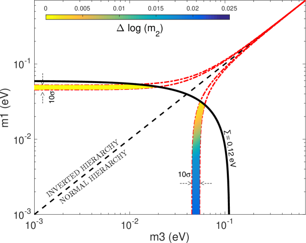
An illustration of the scenario we face is given in Figure 1. The red dashed contours show the region allowed by oscillation data. They represent the two filaments discussed above, but now in projection. Their widths vary considerably since we are in the logarithmic domain (for visual clarity we use a broad contour). The complementarity of the cosmological data is highlighted by the solid black curve, which provides an upper bound on the sum of the three masses eV, thereby truncating the extent of the contours at larger masses. Note that due to freedom in the value of , the sum is not uniquely defined in the plane. What is of interest here is a contour of the surface eV which intersects the filaments. To create this we use the measurement of from equation (3.1) to specify . From this perspective it becomes clear that even with only the oscillation data at hand, before looking at any cosmological data, we should consider it reasonably likely that the sum of the masses is of the order 0.1 eV (i.e., towards the lower limit allowed by oscillation data). This is because towards very large masses, the uncertainty in the measurement corresponds to a vanishingly small interval in . Therefore our posterior on the sum of the masses, , is heavily penalised towards large masses. In stark contrast, if we had adopted an informative uniform prior (i.e., a uniform prior in rather than ), we would have been repeatedly surprised as a sequence of modern cosmological surveys failed to unearth the influence of the neutrino masses.
The crucial factor here is the influence of the third mass parameter , which has been marginalised out in Figure 1. The filaments vary in width in , in much the same manner as can be seen in the other two dimensions. This evolution in depth, , is visually represented by the colour of the shaded areas. In the regime of the normal hierarchy, and for the case of a vanishingly small , the range of permissible values at any given pair is governed by our uncertainty in the quantity , of approximately . Once we reach very low masses, eV, then we settle at a minimum value of eV. Thus the space available within the domain saturates at approximately . Let’s compare this with the available parameter space in the inverted hierarchy. In this case, as we take the limit towards one of the neutrinos being massless, then we are left with eV. This corresponds to a much narrower range, approximately . Thus the sheer volume of parameter space that our data has been able to exclude is highly asymmetric with respect to the plane.
Our posterior belief in the two hypotheses, the inverted hierarchy and the normal hierarchy, relates to the integral of the posterior distribution over their respective areas. Provided our prior is sufficiently broad, each integral is dominated by the low mass regime, where the contours are at maximal thickness. Due to the saturation of , our result becomes completely insensitive to the breadth of our prior. The evidence ratio is well approximated by simply . Thus we ought to favour the normal hierarchy over the inverted hierarchy with odds of . This will strengthen further if cosmological bounds on are imposed, as they penalise the inverted scenario more aggressively than the normal hierarchy, as Fig. 1 illustrates.
We are drawn to this conclusion because the oscillation data have eliminated a highly asymmetric region of parameter space in the logarithmic domain. This may not seem particularly intuitive, so it is instructive to consider similar scenarios where our posterior belief is driven by the volume of the available parameter space. One example mentioned earlier is the identifying the orientation of a concealed stick - this is straightforward to verify numerically. Another analogy which may be helpful to consider is the abundance of measurements whose numerical values start with a “1” or a “9”. An intuitive response might be that they arise with equal frequency, but the reality is that there is almost a seven-fold difference in their respective abundances (in any field of science)111This is known as Benford’s law, which applies to many real-life sets of numerical data [37].. The most straightforward interpretation of this phenomenon is, again, due to the availability of parameter space in the logarithmic domain.
3.3 Mass Degeneracy
It is interesting to consider a hypothetical special case: What would happen if had been perfectly measured to be identically zero? This approximation is often used in cosmology since the solar mass splitting has virtually no observational consequences for cosmological data. Then there is no third dimension to worry about in Figure 1. The value of is defined at each point in the plane, so the shaded area would all be the same colour. And we therefore no longer have any asymmetry between the two hierarchies if we neglect any cosmological information. Our conclusion within this hypothetical scenario would be that both hierarchies are equally probable. In other words, when adopting a logarithmic prior on the mass and setting the solar mass splitting to zero would make the two hierarchies equally likely. Adding a cosmological bound breaks the symmetry and, in particular shows a preference for NH with odds 1.8:1 when . This highlights the importance of performing the model selection analysis with the correct dimensionality in parameters and prior space. It is the smallness of the solar mass splitting (yet the fact that it is non zero) relative to the atmospheric splitting that makes the Occam factor favour the normal hierarchy using this particular prior.
4 Hierarchical model
In the previous section we presented a pedagogical calculation illustrating how the Occam factor strongly favours the normal hierarchy. However the framework was a little too simplistic to allow robust conclusions to be drawn.
Rather than restrict ourselves to a single pre-determined prior, of fixed position and breadth, it is advantageous to work with a hyperprior. In practice we introduce an entire family of priors and effectively marginalises over them. Hyperpriors are more flexible and make the posterior less sensitive to the prior itself. We shall operate in a five-dimensional parameter space, consisting of the three neutrino masses (for brevity we shall denote the mass vector ), and two hyperparameters and (see e.g.,[38, 39, 40]), as follows
| (4.1) |
Here represents the data vector and the hypothesis i.e., normal or inverted hierarchy, and is the hyperprior.
To reiterate, the prior ought to reflect our state of belief before the data arrived. The three masses are indistinguishable before the data arrives, so our prior must reflect this symmetry. This feature is also known as exchangeability. We note that this condition is satisfied if the three masses share a common origin, a hypothesis that is adopted in many models for the neutrino masses. So we shall consider that three masses, , , are drawn from a common prior. Then, based on their relative sizes, these three masses are assigned to , and , as defined earlier. In order to specify the position and breadth of the prior, we shall introduce the variables and which control the mean and standard deviation respectively. This specifies the prior on each mass before any ordering takes place. Thus the prior propagated through to will tend to prefer lighter masses values than the effective prior on . Further we adopt a prior of the form
| (4.2) |
where denotes the normal, Gaussian, distribution. For the purposes of performing Bayesian model selection, the quantity which we seek to evaluate is the evidence, . The inference procedure may then be decomposed into the following tiers, as is characteristic of Bayesian hierarchical models.
| (4.3) |
| (4.4) |
Note that our analysis differs significantly from that of Ref. [12]. Although not stated explicitly, they appear to make the following identification for the case of the normal hierarchy (where takes on the role of the lightest neutrino),
| (4.5) |
denotes the Dirac delta function. The relation above implicitly assumes that informative uniform priors are imposed upon both and . This disproportionately favours masses with a value close to an imposed upper bound. To illustrate the potential issues which can arise with informative priors, imagine applying the same technique to other sets of particles within the Standard Model. How should we proceed if we did not know the absolute values of any quark or lepton masses, but were given approximate values of their mass splittings and the sums of their masses. In each case, our estimation of the up, down, and electron masses would be heavily biased, since they lie several orders of magnitude below their heavier counterparts. Likewise, in the current circumstance, the lightest neutrino could be several orders of magnitude below eV. Theoretical considerations set the minimum viable neutrino mass at approximately eV [41]. A different approach, which we do not explore here, is to introduce a discrete hyperparameter which assigns equal odds to the two hierarchies given the mass splitting obtained from oscillations constraints (an a posteriori decision, rather than a fundamental prior). This is for example discussed in [14] where the uncertainty on the mass splitting is neglected and a linear, improper, prior on the mass of the lightest neutrino is adopted.
4.1 Methodology
Here we briefly outline the procedure we use to numerically evaluate the likelihood of the hyperparameters .
-
1.
For a given value of and , this defines a probability distribution from which we draw sets of three samples. For each set of three, the masses are ranked from smallest to largest, here we shall designate these ranks as , , and .
-
2.
For each set we compute the following four quantities: ; ; ; and .
-
3.
In order to determine the likelihood of the two hyperparameters, we compute the inner integral of equation . For the case of the normal hierarchy this becomes
(4.6) Here denotes the mass vector of the th random sample, while the terms represent the different components of the data vector. For example, represents the measurement of as derived from cosmological density perturbations.
-
4.
Repeat Step 3 for the case of the inverted hierarchy. This involves a reinterpretation of the squared mass splittings as follows
-
5.
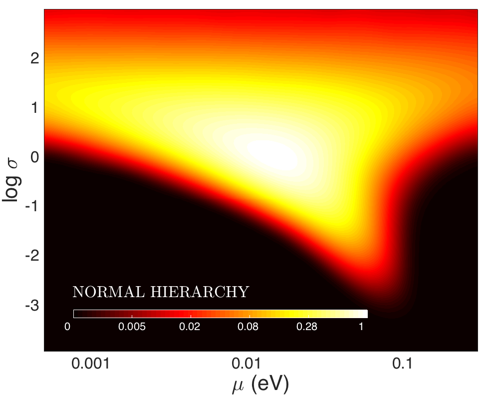
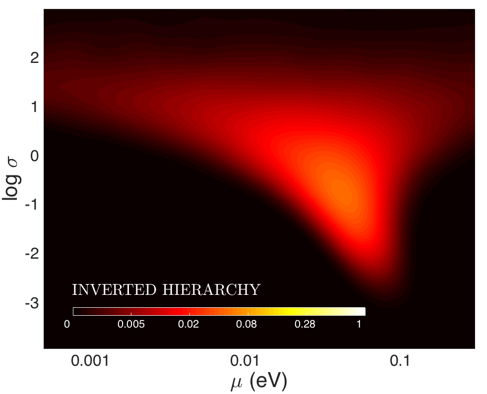
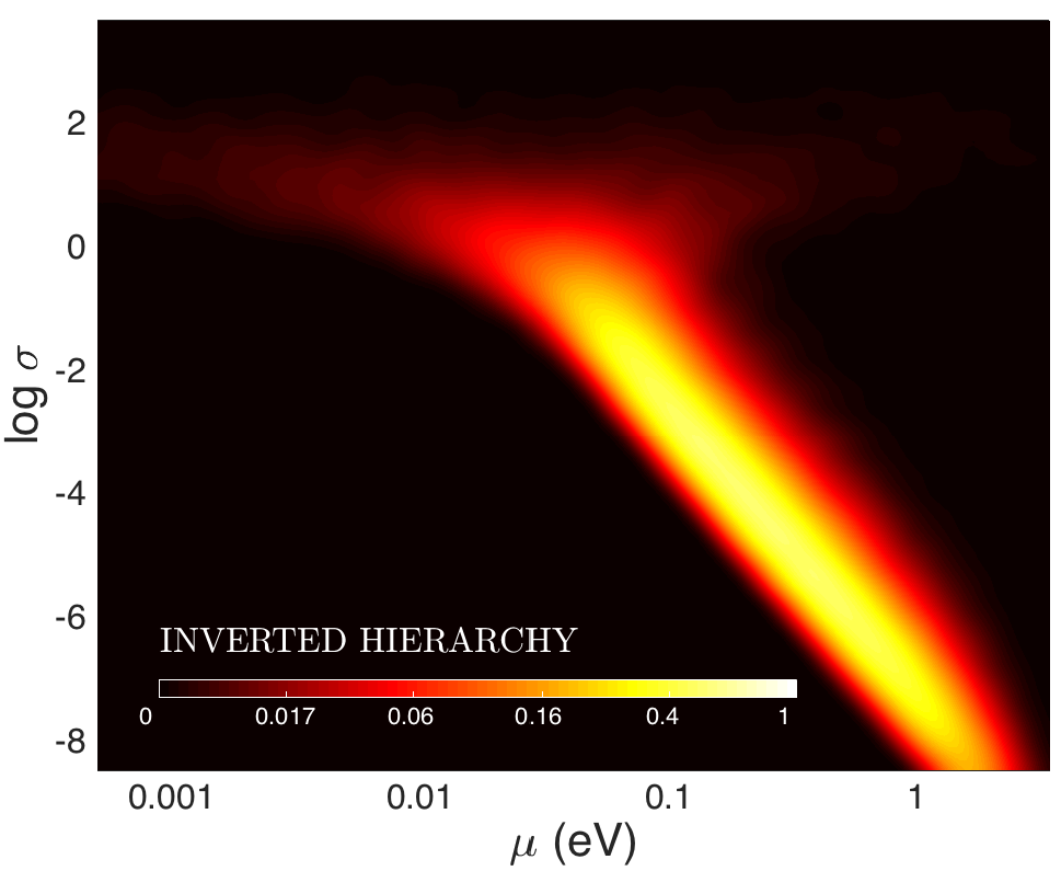
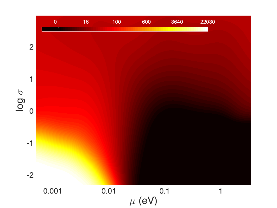
Repeat Steps 1-4 for 100 x 100 different values of and , across a logarithmically spaced grid. This yields the joint probability distribution shown in Figure 2. The prior is uniform across this region, therefore all of the visible structure has been imposed by the dataset.
In order to test our numerical precision, we repeated this procedure with a smaller number of samples, . This was found to modify the resultant Bayes factors by less than .
5 Results
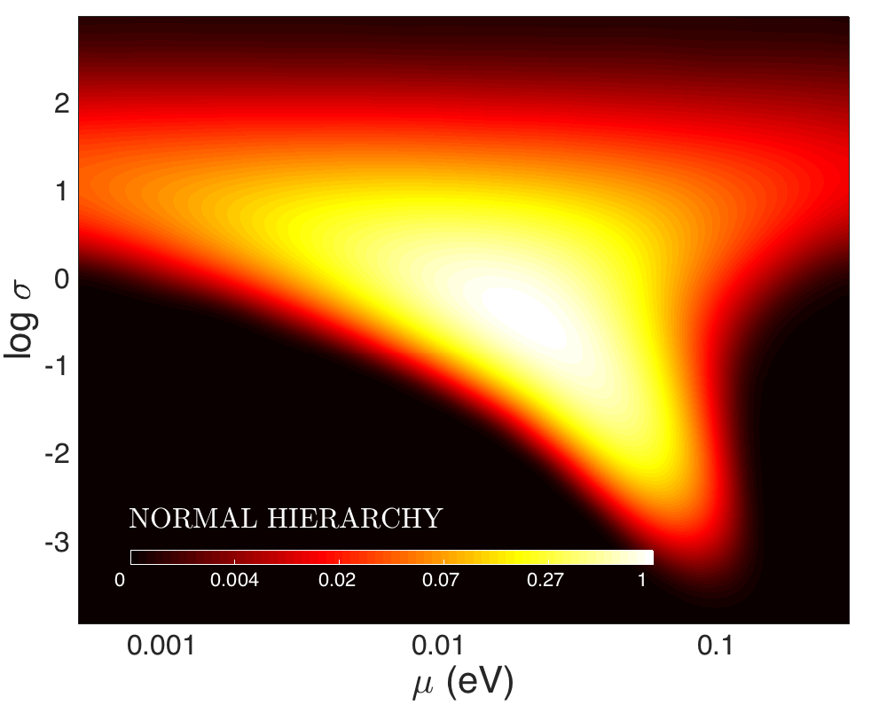
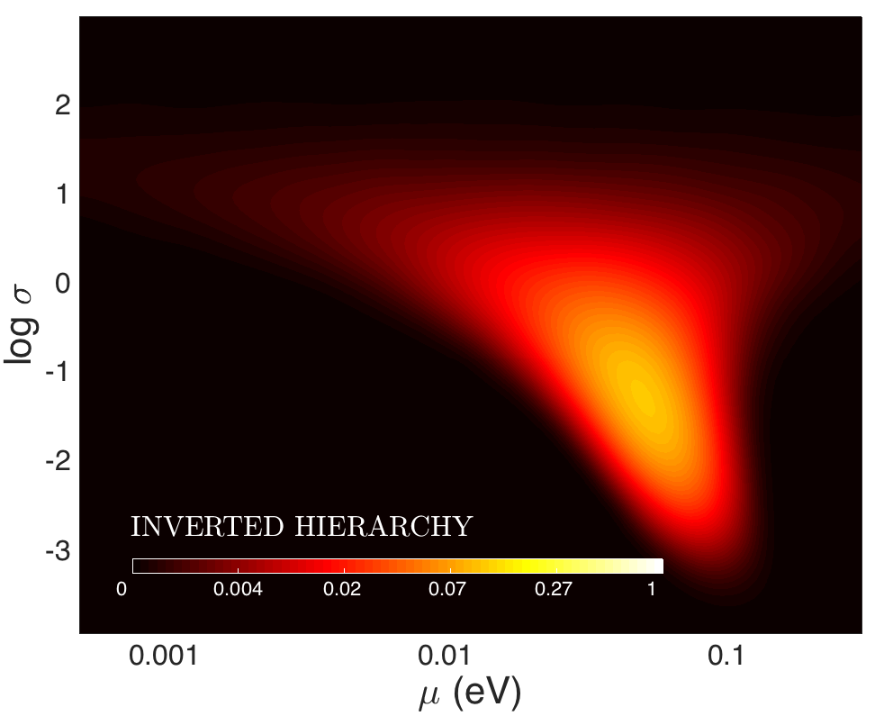
Figure 2 illustrates the evidence for the hyperparameters, . The left hand panel corresponds to the case of the normal hierarchy. Low values of are disfavoured by the requirement of a significant mass splitting. Meanwhile very large values of are penalised because they are less predictive. Cosmological information provides the third boundary, eliminating the largest values of . Nonetheless a substantial area of parameter space retains a high likelihood. By contrast, in the right hand panel we see the region of parameter space associated with the inverted hierarchy. For a linear colour scale the features are barely visible, so here we introduce a logarithmic scale. The likelihood suffers both in terms of its peak value (the maximum is a factor of fifteen lower than in the normal hierarchy) and in terms of its confinement to a more restricted region of parameter space.
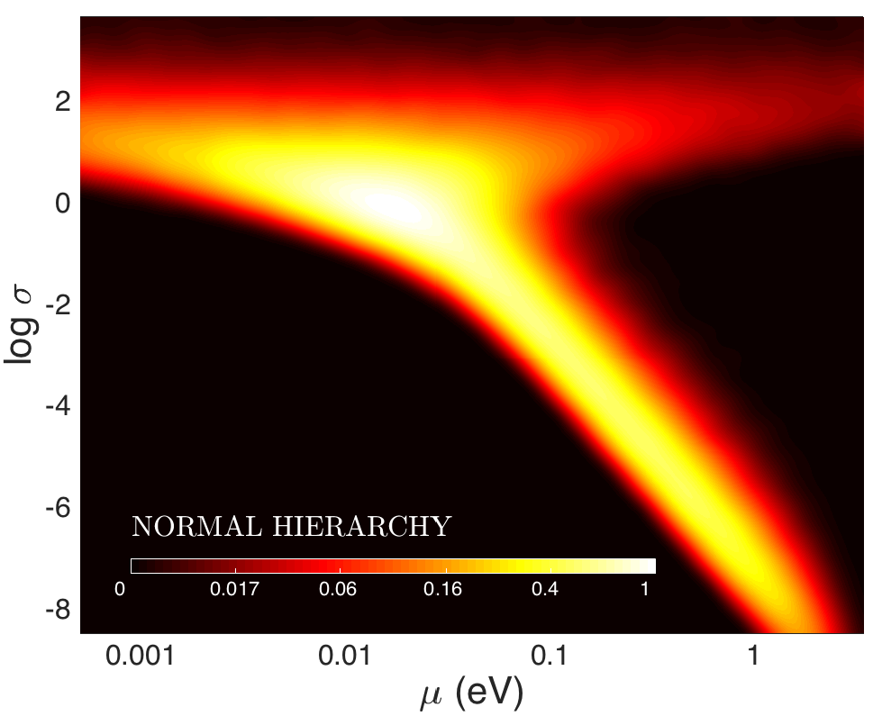
Another striking feature of Figure 2 is that ratio between the two panels, at any given point in the plane, favours the NH. So we should anticipate that our results are not particularly sensitive to our choice of hyperprior, . For comparison, in Fig. 3 we show the corresponding distribution without imposing the cosmological bound. The comparison of Figs. 2 and 3, clearly illustrates how cosmology has wiped out the space available for the inverted hierarchy.
5.1 Bayesian Evidence
Our posterior belief in the two hypotheses, the normal and inverted orderings, is given by
| (5.1) |
In principle we are free to introduce a bias in the ratio , but here we consider the prior probabilities of the two models to be equal. The important quantity in influencing the strength of our posterior belief is therefore the evidence ratio, , also known as the Bayes factor defined in equation (2.3). This quantity is evaluated using equation (4.3), while again employing an uninformative prior , as given by
|
|
(5.2) |
where denotes the uniform distribution. For computational purposes we set hard bounds of and , broadening either of these limits has no impact on our results. Provided an upper bound is placed on the sum of masses, in addition to the mass splittings, then the data is capable of restricting the marginal likelihood associated with the hyperpriors to a finite range. We begin by noting that in the absence of neutrino oscillation data, i.e, setting the uncertainties of the mass splittings to be infinite, then our priors yield odds of the two hierarchies of precisely 1 : 1. In fact this is a generic feature of any prior that is invariant to permutations of its elements, i.e. , as this ensures .
Figure 4 illustrates how the evidence ratio changes as we traverse the plane. Here we make use of data from neutrino oscillations. Note that for broader distributions, , we consistently find evidence values of is agreement and analogy with the findings of Sec. 3.2.
In Table 1 we present the Bayesian evidence for a range of different degrees of precision for the sum of the neutrino masses. Hereafter, for the classification of the evidence, we refer to the slightly modified Jeffreys’ scale [42] as discussed in [43]. When only utilising data from neutrino oscillations, there is no significant evidence for one hierarchy over the other, being classified as “Weak”. This result is qualitatively different from that obtained in Sec. 3.2 where a simple log prior was used and highlights the usefulness of introducing the hyperprior. The current robust limit eV from [3] already provides odds of approximately 42:1, which translate into strong evidence in favour the normal hierarchy. Note that, if we instead use the Ly- limit, eV, the odds increase to 50:1, if we also include the latest measurement of the Hubble constant [27] the odds increase to 90:1. Thus in this approach, the cosmological bound on is critical in driving the evidence in favour of the normal hierarchy.
5.2 Sensitivity Analysis
In order to explore our sensitivity to the choice of prior , we shall now impose an informative prior on . Figure 5 shows the impact of adopting a hyperprior of the form . This favours narrower distributions, which in turn slightly weakens the extent to which the NH is favoured over IH. For the illustrated example we set eV, leaving us with odds of . Meanwhile eV returns odds of .
We conducted a further sensitivity test by replacing the normal distribution with a top hat distribution, described by the same set of parameters and . This was found to have a minimal impact on the evidence ratios.
6 Discussion and conclusions
By performing a likelihood analysis in its full three-dimensional parameter space, and adopting a minimally informative hierarchical model, we demonstrate that the inverted hierarchy suffers from a much more extensive exclusion of its parameter space than the normal hierarchy. This can be largely attributed to the residual freedom in the mass of in the logarithmic domain. Central to this result is the cosmological bound on the sum of the neutrino masses. Without this information, the Bayesian evidence is weak, and does not significantly favour one ordering over the other, as it is apparent from Tab. 1 and 2. As with all applications of Bayesian model selection, there is some dependence on the choice of adopted prior. Nonetheless, we can draw some robust conclusions which have several broad implications.
6.1 Implications in neutrino physics
The determination of the nature of neutrinos, whether Majorana or Dirac fermions, is a major long-term unsolved problem in particle physics, with double beta decay experiments being the most sensitive probes to solve this riddle. These experiments could prove the existence of a rare double beta decay of nuclei without neutrino emission, a decay which is mediated by the internal exchange of the light Majorana neutrinos (other beyond the standard model physics may also contribute to the decay). In the minimal case, the expected half-lives of neutrino-less double beta decays of nuclei depend on nuclear physics dynamics and on the neutrino mass scale and hierarchy. In fact, the neutrino mass hierarchy plays a key role in identifying the largest half-lives to be explored [44]. In our opinion, the results derived in this work are very relevant to the development of next generation double beta decay future experiments. While it is true that, independently of the neutrino mass hierarchy, the discovery could be close to the upper bounds, for example 1027 yr for Xe [45], the strong evidence for the normal neutrino mass hierarchy favours experimental techniques with potential to reach multi-ton active mass detectors and meet the requirements of very low background with, for example, topological signatures[46, 47].
Our results have also important implications for neutrino oscillation experiments and neutrino mass models. Neutrino mass hierarchy is among the physics goals of several proposed neutrino detectors [48, 49, 50, 51, 52]. Experiments whose major scientific goal is the identification of the neutrino mass hierarchy are particularly affected by the conclusions of this paper. In particular, according to our findings, experiments with observables more sensitive to normal mass hierarchy are much more likely to yield a successful outcome.
| (eV) 95% | ||||||||
|---|---|---|---|---|---|---|---|---|
| Odds (NH/IH) | 6500:1 | 95:1 | 53:1 | 42:1 | 31:1 | 18:1 | 7:1 | 2.6:1 |
| 9 | 4.5 | 4.0 | 3.7 | 3.4 | 2.9 | 1.9 | 1.0 | |
| Classification | Very Strong | Strong | Strong | Strong | Strong | Positive | Positive | Weak |
| (eV) 95% | |||||||
|---|---|---|---|---|---|---|---|
| Odds (NH/IH) | 225:1 | 33:1 | 24:1 | 18:1 | 13:1 | 6.3:1 | 2.6:1 |
| 5.4 | 3.5 | 3.2 | 2.9 | 2.5 | 1.8 | 1.0 | |
| Classification | Very Strong | Strong | Strong | Positive | Positive | Positive | Weak |

6.2 Interpreting results from upcoming surveys
Fig. 6 serves as guidance for the interpretation of forthcoming results from cosmology. In order to facilitate a comparison with conventional cosmological analyses, we present our results in terms of the confidence bounds which would be achieved when imposing a uniform prior on , and without utilising external information from neutrino oscillation experiments. The solid line corresponds to the family of Gaussian likelihoods , of varying standard deviation but each with maxima located at eV, as motivated by the findings of recent analyses. Meanwhile the dashed line demonstrates the impact of shifting the maximum likelihood value to eV. These lines illustrate the degree of belief we would reach in the normal neutrino hierarchy, when this hypothetical cosmological data is combined with the squared mass splittings presented in Section 3.1. They were computed by interpolating the values of Tab. 1, shown as symbols. What if these hypothetical future measurements provide instead a likelihood for which is centred at a value close to the current 95% upper limit? In this case, if this value is e.g., eV, the preference for normal hierarchy is much weaker but still a preference remains. For example for 1- errors of eV corresponding to 95% upper limits of eV, one would obtain odds of to 1 in favour of NH.
6.3 Constraints on the individual masses
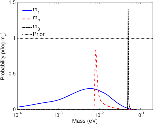
Figure 7 presents the posterior distributions on the three individual neutrino masses. In light of our findings in the previous section, here we only consider the normal hierarchy’s contribution to the posterior. Unsurprisingly the lightest mass is the least well constrained, with a mild preference that it is not very far in log space from the other two masses. Meanwhile the two heavier masses, and , possess sharper but highly asymmetric posteriors. From these posterior distributions we may derive medians and credible intervals for each mass eigenstate, yielding ( CL).
Finally, the dotted horizontal line illustrates our belief in each of the masses before the data arrives. We stress that the difference between the prior and the posterior distribution is unequivocally driven by the data.
6.4 Constraints on the sum of the masses
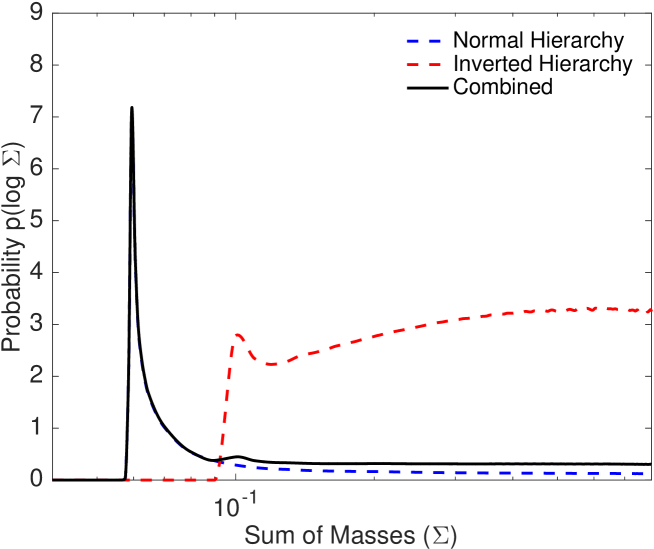
In order to perform a rigorous inference of cosmological parameters, by exploiting data from cosmological surveys, it is necessary to ascribe a prior on the sum of the neutrino masses . For example, the Planck team either assign a fixed fiducial value of eV, or explore a uniform prior. However, note that even a uniform prior on the three individual masses would not yield a uniform prior on the sum. Here we advocate that the posterior distribution from the oscillation experiments should form the basis of our prior for cosmological surveys. In Figure 8 we illustrate this distribution, given as a weighted sum of the two components, specifically
| (6.1) |
The red and blue dashed lines illustrate and respectively, while the solid line depicts their weighted combination . Here our data vector is comprised of the two measured mass splittings, and the bound on derived from laboratory experiments (i.e., no cosmological information). This leads an odds ratio between the two hierarchies of . Since is potentially useful for future analyses of cosmological data, it has been made publicly available222At the following URL: https://github.com/frgsimpson/neutrino-priors.
By introducing additional cosmological information, the sum of the masses can also be resolved, Our fiducial Gaussian bound of eV yields meV. The mode of the posterior distribution lies significantly below the quoted median value, at meV. As before, this posterior is composed of two distinct contributions from the normal and inverted hierarchies. The measurement does not drastically change in the case of the normal hierarchy: meV. Meanwhile the inverted hierarchy continues to prefer considerably larger values, meV (all 95% credible intervals).
Figure 8 also provides us with another perspective on how the cosmological data’s preference for the normal hierarchy arose. Once the mass splittings were measured, the inverted hierarchy much prefers larger values of , and it is this regime which has now been largely excluded by cosmological data.
6.5 Conclusions
We have presented a joint analysis of data on the masses of the three neutrinos, using Bayesian hierarchical modelling. We find that the combination of laboratory and cosmological measurements already provide strong evidence in favour of a normal hierarchy. The complementarity of these datasets also permit an inference of the individual masses, , and their sum meV ( credible intervals).
The extent to which our belief in the inverted hierarchy diminishes is related to the collapse in its available parameter space. Within the context of the inverted hierarchy, only contrived combinations of neutrino masses remain compatible with the data. While this effect has been known to exist in a one-dimensional context, here we have demonstrated that the effect is significantly amplified when accounting for the full three-dimensional domain. Our results differ (quantitatively, not qualitatively) from those of Refs. [12, 13] who use an informative uniform prior and find that the odds for NH:IH are about 2:1 or 3:1, only, depending on the dataset combination. Such a prior tends to favour high masses, prohibiting the masses from possessing significant variance in the logarithmic domain. When dealing with parameters whose uncertainty spans several orders of magnitude, such as in this case, we argue that a less informative prior should be adopted.
Due to the differences in parameter space, the first significant digit of a given neutrino mass is much more likely to be a ‘1’ than a ‘9’, in accordance with Benford’s law. This may at first seem unintuitive, yet it is incontrovertible. One does not require knowledge of the formation mechanism in order to make this statement. In a similar vein, the mass hierarchy is very much more likely to be normal rather than inverted. We also found a slight preference for the lightest mass to be smaller than 5 meV. These results, light smallest mass and normal hierarchy, agree well with predictions derived by, among other models, minimal SO(10) grand unified models [53].
Is there a means by which our conclusion can be evaded? One can always resort to invoking unknown systematics large enough to invalidate the observational data, or hoping that the CDM cosmological model is wildly inaccurate, but these appear to be highly speculative escape routes. As always, our posterior belief is to some extent influenced by our choice of prior. In this work we employed a minimally informative prior, and demonstrated that modest modifications to the prior impart only a minor impact on the evidence ratios. One could construct a more contrived set of priors which strongly favour inverted orderings. Or equivalently, one could amplify the prior on the hypothesis itself . However there appears no clear justification for either of these actions.
Acknowledgements.— This work is supported by Generalitat Valencia Prometeo Grant II/2014/050, by the Spanish Grants FPA2011-29678 of MINECO and by PITN- GA-2011-289442-INVISIBLES. Funding for this work was partially provided by the Spanish MINECO under projects AYA2014-58747-P and MDM-2014-0369 of ICCUB (Unidad de Excelencia ‘María de Maeztu’).
References
- [1]
- [2] M. C. Gonzalez-Garcia, M. Maltoni, and T. Schwetz, JHEP 11, 052 (2014), 1409.5439.
- [3] A. J. Cuesta, V. Niro, and L. Verde, Physics of the Dark Universe 13, 77 (2016), 1511.05983.
- [4] A. Osipowicz et al. (KATRIN) (2001), hep-ex/0109033.
- [5] B. Monreal and J. A. Formaggio, Phys. Rev. D80, 051301 (2009), 0904.2860.
- [6] P. J. Doe et al. (Project 8), in Proceedings, Community Summer Study 2013: Snowmass on the Mississippi (CSS2013): Minneapolis, MN, USA, July 29-August 6, 2013 (2013), 1309.7093, URL https://inspirehep.net/record/1255861/files/arXiv:1309.7093.pdf.
- [7] N. Palanque-Delabrouille, C. Yèche, J. Baur, C. Magneville, G. Rossi, J. Lesgourgues, A. Borde, E. Burtin, J.-M. LeGoff, J. Rich, M. Viel, and D. Weinberg, JCAP 11, 011 (2015), 1506.05976.
- [8] C. Carbone, L. Verde, Y. Wang, and A. Cimatti, JCAP 1103, 030 (2011), 1012.2868.
- [9] B. Audren, J. Lesgourgues, S. Bird, M. G. Haehnelt, and M. Viel, JCAP 1301, 026 (2013), 1210.2194.
- [10] J. Hamann, S. Hannestad, and Y. Y. Y. Wong, JCAP 1211, 052 (2012), 1209.1043.
- [11] R. Jimenez, T. Kitching, C. Pena-Garay, and L. Verde, JCAP 1005, 035 (2010), 1003.5918.
- [12] S. Hannestad and T. Schwetz, JCAP 11, 035 (2016), 1606.04691.
- [13] S. Vagnozzi, E. Giusarma, O. Mena, K. Freese, M. Gerbino, S. Ho, and M. Lattanzi, ArXiv e-prints (2017), 1701.08172.
- [14] M. Gerbino, M. Lattanzi, O. Mena, and K. Freese, ArXiv e-prints (2016), 1611.07847.
- [15] J. Lesgourgues and S. Pastor, Phys. Rept. 429, 307 (2006), astro-ph/0603494.
- [16] J. R. Bond, G. Efstathiou, and J. Silk, Phys. Rev. Lett. 45, 1980 (1980).
- [17] J. Brandbyge and S. Hannestad, JCAP 1001, 021 (2010), 0908.1969.
- [18] C. Wagner, L. Verde, and R. Jimenez, Astrophys. J. 752, L31 (2012), 1203.5342.
- [19] S. Bird, M. Viel, and M. G. Haehnelt, Mon. Not. Roy. Astron. Soc. 420, 2551 (2012), 1109.4416.
- [20] W. Hu, D. J. Eisenstein, and M. Tegmark, Physical Review Letters 80, 5255 (1998), astro-ph/9712057.
- [21] J. Lesgourgues, S. Pastor, and L. Perotto, PRD 70(4), 045016 (2004), hep-ph/0403296.
- [22] S. Wang, Z. Haiman, W. Hu, J. Khoury, and M. May, Physical Review Letters 95(1), 011302 (2005), astro-ph/0505390.
- [23] M. Takada, E. Komatsu, and T. Futamase, PRD 73(8), 083520 (2006), astro-ph/0512374.
- [24] S. Hannestad and Y. Y. Y. Wong, JCAP 7, 004 (2007), astro-ph/0703031.
- [25] T. D. Kitching, A. F. Heavens, L. Verde, P. Serra, and A. Melchiorri, PRD 77(10), 103008 (2008), 0801.4565.
- [26] P. A. R. Ade et al. (Planck) (2015), %****␣hierarchy_v3.tex␣Line␣625␣****1502.01589.
- [27] A. G. Riess, L. M. Macri, S. L. Hoffmann, D. Scolnic, S. Casertano, A. V. Filippenko, B. E. Tucker, M. J. Reid, D. O. Jones, J. M. Silverman, R. Chornock, P. Challis, et al., ApJ 826, 56 (2016), 1604.01424.
- [28] E. Giusarma, M. Gerbino, O. Mena, S. Vagnozzi, S. Ho, and K. Freese, PRD 94(8), 083522 (2016), 1605.04320.
- [29] E. Di Valentino, E. Giusarma, O. Mena, A. Melchiorri, and J. Silk, PRD 93(8), 083527 (2016), 1511.00975.
- [30] R. de Putter, E. V. Linder, and A. Mishra, Phys. Rev. D89(10), 103502 (2014), 1401.7022.
- [31] T. Namikawa, S. Saito, and A. Taruya, JCAP 1012, 027 (2010), 1009.3204.
- [32] M. Baldi, F. Villaescusa-Navarro, M. Viel, E. Puchwein, V. Springel, and L. Moscardini, MNRAS 440, 75 (2014), 1311.2588.
- [33] R. Jimenez, T. Kitching, C. Peña-Garay, and L. Verde, JCAP 5, 035 (2010), 1003.5918.
- [34] D. J. MacKay, Information theory, inference and learning algorithms (Cambridge university press, 2003).
- [35] B. S. Clarke and A. R. Barron, Journal of Statistical planning and Inference 41(1), 37 (1994).
- [36] S. Weinberg, Physical Review Letters 59, 2607 (1987).
- [37] B. Benford, Proc. Am. Philos. Soc 78, 551 572 (1938).
- [38] G. C. Tiao and G. E. Box, The American Statistician 27(1), 12 (1973).
- [39] D. J. MacKay, in Maximum entropy and Bayesian methods (Springer, 1996), pp. 43–59.
- [40] M. Hobson, S. Bridle, and O. Lahav, Monthly Notices of the Royal Astronomical Society 335(2), 377 (2002).
- [41] S. Davidson, G. Isidori, and A. Strumia, Physics Letters B 646(2), 100 (2007).
- [42] H. Jeffrey, The theory of probability (Oxford University Press, 1961).
- [43] K. R. E. and R. A. E., Journal of the American Statistical Association 430, 773 (1995).
- [44] H. Murayama and C. Pena-Garay, Phys. Rev. D69, 031301 (2004), hep-ph/0309114.
- [45] A. Gando et al. (KamLAND-Zen), Phys. Rev. Lett. 117(8), 082503 (2016), [Addendum: Phys. Rev. Lett.117,no.10,109903(2016)], 1605.02889.
- [46] F. Granena et al. (NEXT) (2009), 0907.4054.
- [47] A. E. Chavarria, C. Galbiati, X. Li, and J. A. Rowlands (2016), 1609.03887.
- [48] K. Abe et al. (Hyper-Kamiokande Proto-Collaboration), PTEP 2015, 053C02 (2015), 1502.05199.
- [49] R. Acciarri et al. (DUNE) (2015), 1512.06148.
- [50] F. An et al. (JUNO), J. Phys. G43(3), 030401 (2016), 1507.05613.
- [51] M. G. Aartsen et al. (IceCube) (2016), 1607.02671.
- [52] S. Adrian-Martinez et al. (KM3Net), J. Phys. G43(8), 084001 (2016), 1601.07459.
- [53] F. Buccella, M. Chianese, G. Mangano, G. Miele, S. Morisi, and P. Santorelli (2017), 1701.00491.