Updated fit to three neutrino mixing: status of leptonic CP violation

Abstract

We present a global analysis of solar, atmospheric, reactor and accelerator neutrino data in the framework of three-neutrino oscillations based on data available in summer 2014. We provide the allowed ranges of the six oscillation parameters and show that their determination is stable with respect to uncertainties related to reactor neutrino and solar neutrino flux predictions. We find that the maximal possible value of the Jarlskog invariant in the lepton sector is $0.0329\pm 0.0009$ ($\mathrel{\pm}0.0027$) at the $1\sigma$ ($3\sigma$) level and we use leptonic unitarity triangles to illustrate the ability of global oscillation data to obtain information on CP violation. We discuss “tendencies and tensions” of the global fit related to the octant of $\theta_{23}$ as well as the CP violating phase $\delta_{\text{CP}}$. The favored values of $\delta_{\text{CP}}$ are around $3\pi/2$ while values around $\pi/2$ are disfavored at about $\Delta\chi^{2}\simeq 6$. We comment on the non-trivial task to assign a confidence level to this $\Delta\chi^{2}$ value by performing a Monte Carlo study of T2K data.

1 Introduction

Thanks to remarkable discoveries by a number of neutrino oscillation experiments it is now an established fact that neutrinos have mass and leptonic flavors are not symmetries of Nature Pontecorvo:1967fh ; Gribov:1968kq , see Ref. GonzalezGarcia:2007ib for an overview. Ignoring controversial indications for the existence of neutrino mass states at the eV scale (see Ref. Kopp:2013vaa and references therein) a consistent description of global data on neutrino oscillations is possible by assuming mixing among the three known neutrinos ($\nu_{e}$, $\nu_{\mu}$, $\nu_{\tau}$), which can be expressed as quantum superpositions of three massive states $\nu_{i}$ ($i=1,2,3$) with masses $m_{i}$. This implies the presence of a leptonic mixing matrix in the weak charged current interactions Maki:1962mu ; Kobayashi:1973fv which can be parametrized as PDG :

$$U=\begin{pmatrix}c_{12}c_{13}&s_{12}c_{13}&s_{13}e^{-i\delta_{\text{CP}}}\\ -s_{12}c_{23}-c_{12}s_{13}s_{23}e^{i\delta_{\text{CP}}}&\hphantom{+}c_{12}c_{23}-s_{12}s_{13}s_{23}e^{i\delta_{\text{CP}}}&c_{13}s_{23}\\ \hphantom{+}s_{12}s_{23}-c_{12}s_{13}c_{23}e^{i\delta_{\text{CP}}}&-c_{12}s_{23}-s_{12}s_{13}c_{23}e^{i\delta_{\text{CP}}}&c_{13}c_{23}\end{pmatrix},$$ (1)

where $c_{ij}\equiv\cos\theta_{ij}$ and $s_{ij}\equiv\sin\theta_{ij}$. In addition to the Dirac-type phase $\delta_{\text{CP}}$, analogous to that of the quark sector, there may also be two physical phases associated to a possible Majorana character of neutrinos, which however are not relevant for neutrino oscillations Bilenky:1980cx ; Langacker:1986jv and are therefore omitted in the present work. Given the observed hierarchy between the solar and atmospheric mass-squared splittings there are two possible non-equivalent orderings for the mass eigenvalues, which are conventionally chosen as

$$\Delta m^{2}_{21} \ll\hphantom{+}(\Delta m^{2}_{32}\simeq\Delta m^{2}_{31}>0)\,;$$ (2)

$$\Delta m^{2}_{21} \ll-(\Delta m^{2}_{31}\simeq\Delta m^{2}_{32}<0)\,,$$ (3)

with $\Delta m^{2}_{ij}\equiv m_{i}^{2}-m_{j}^{2}$. As it is customary we refer to the first option, Eq. (2), as Normal Ordering (NO), and to the second one, Eq. (3), as Inverted Ordering (IO); in this form they correspond to the two possible choices of the sign of $\Delta m^{2}_{31}$. In this convention the angles $\theta_{ij}$ can be taken without loss of generality to lie in the first quadrant, $\theta_{ij}\in[0,\pi/2]$, and the CP phase $\delta_{\text{CP}}\in[0,2\pi]$. In the following we adopt the (arbitrary) convention of reporting results for $\Delta m^{2}_{31}$ for NO and $\Delta m^{2}_{32}$ for IO, i.e., we always use the one which has the larger absolute value. Sometimes we will generically denote such quantity as $\Delta m^{2}_{3\ell}$, with $\ell=1$ for NO and $\ell=2$ for IO.

In this article, we present an up-to-date (as of summer 2014) global analysis of solar, atmospheric, reactor and accelerator neutrino data in the framework of three-neutrino oscillations. Alternative recent global fits have been presented in Refs. Capozzi:2013csa ; Forero:2014bxa . In Sec. 2 we describe the data used in our analysis (listed also in Appendix A) and we present the results of the global analysis and the allowed ranges of the oscillation parameters. In Sec. 3 we focus on our knowledge on CP violation, discussing the present status of the leptonic Jarlskog invariant and displaying the results of our fit in terms of leptonic unitarity triangles. In Sec. 4 we comment on various “tensions and tendencies” in the global data, including the reactor anomaly, the tension in the $\Delta m^{2}_{21}$ determination from solar experiments versus KamLAND, the determination of $\Delta m^{2}_{31}$, tendencies in fit results for $\theta_{23}$ and $\delta_{\text{CP}}$, and statistical issues related to the determination of the CP violating phase $\delta_{\text{CP}}$. Finally in Sec. 5 we present our conclusions.

The numerical results of our analysis as well as figures are available at the website nufit , where also one- and two-dimensional $\chi^{2}$ tables are available for download. Furthermore, this website will be kept up-to-date when new data becomes available.

2 Oscillation parameters: results of the global analysis

2.1 Data included in our analysis

We include in our global analysis the results from Super-Kamiokande atmospheric neutrino data from phases SK1–4 skatm:nu2014 , adding the 1775 days of phase SK4 to their published results on phases SK1–3 Wendell:2010md . Concretely, we consider sub-GeV and multi-GeV $e$-like and $\mu$-like fully contained events, as well as partially contained, stopping and through-going $\mu$ data, each divided into 10 angular bins. Hence we have a total of 70 energy and zenith angle bins. For what concerns disappearance results from long baseline accelerator experiments (LBL) we use the energy distribution of events from MINOS in both $\nu_{\mu}$ ($\bar{\nu}_{\mu}$) disappearance with $10.71~{}(3.36)\times 10^{20}$ protons on target (pot) Adamson:2013whj , which amounts to 39 (14) data points, and from T2K in $\nu_{\mu}$ disappearance Abe:2014ugx with $6.57\times 10^{20}$ pot (16 data points). For LBL appearance results we include both the neutrino and antineutrino events from MINOS Adamson:2013ue , with exposure $10.6\times 10^{20}$ and $3.3\times 10^{20}$ pot, respectively, and from T2K in $\nu_{e}$ appearance Abe:2013hdq with $6.57\times 10^{20}$ pot; each of these samples contributes 5 data points.

In the analysis of solar neutrino experiments we include the total rates from the radiochemical experiments Chlorine Cleveland:1998nv , Gallex/GNO Kaether:2010ag and SAGE Abdurashitov:2009tn . For real-time experiments we include the results from on electron scattering (ES) from the four phases in Super-Kamiokande: the 44 data points of the phase I (SK1) energy-zenith spectrum Hosaka:2005um , the 33 (42) data points of the full energy and day/night spectrum in phase II (III), SK2 Cravens:2008aa (SK3 Abe:2010hy ), and the 24 data points of the energy spectrum and day-night asymmetry of the 1669-day of phase IV, SK4 sksol:nu2014 . The results of the three phases of SNO are included in terms of the parametrization given in their combined analysis Aharmim:2011vm which amount to 7 data points. We also include the main set of the 740.7 days of Borexino data Bellini:2011rx as well as their high-energy spectrum from 246 live days Bellini:2008mr . In the analysis of solar neutrino data we use the GS98 version of the solar standard model Serenelli:2009yc (see Sec. 4.2).

For oscillation signals at reactor experiments we include data from the finalized experiments CHOOZ Apollonio:1999ae (energy spectrum data, 14 data points) and Palo Verde Piepke:2002ju (total rate) together with the spectrum from Double Chooz with 227.9 days live time Abe:2012tg (18 data points), and the 621-day spectrum from Daya Bay db:nu2014 (36 data points), as well as the near and far rates observed at RENO with 800 days of data-taking reno:nu2014 (2 data points with free normalization). We also include the observed energy spectrum in KamLAND data sets DS-1 and DS-2 Gando:2010aa with a total exposure of $3.49\times 10^{32}$ target-proton-year (2135 days). Although reactor experiments with baselines $\lesssim 100$ m do not contribute to oscillation physics, they play an important role in constraining the unoscillated reactor neutrino flux. For this purpose we consider also data from Bugey4 Declais:1994ma , ROVNO4 Kuvshinnikov:1990ry , Bugey3 Declais:1994su , Krasnoyarsk Vidyakin:1987ue ; Vidyakin:1994ut , ILL Kwon:1981ua , Gösgen Zacek:1986cu , SRP Greenwood:1996pb , and ROVNO88 Afonin:1988gx , to which we refer as reactor short-baseline experiments (RSBL). Details on the RSBL analysis can be found in Kopp:2013vaa .

For convenience a detailed list of all the data used in our global analysis can also be found in Appendix A.

2.2 Description of the results

Figure 1: Global $3\nu$ oscillation analysis. Each panel shows a two-dimensional projection of the allowed six-dimensional region after minimization with respect to the undisplayed parameters. The different contours correspond to $1\sigma$, 90%, $2\sigma$, 99% and $3\sigma$ CL (2 dof). Full regions correspond to the analysis with free normalization of reactor fluxes and data from short-baseline (less than 100 m) reactor experiments included. For void regions short-baseline reactor data are not included but reactor fluxes as predicted in Huber:2011wv are assumed. Note that as atmospheric mass-squared splitting we use $\Delta m^{2}_{31}$ for NO and $\Delta m^{2}_{32}$ for IO. The regions in the lower 4 panels are based on a $\Delta\chi^{2}$ minimized with respect to NO and IO.

Figure 2: Global $3\nu$ oscillation analysis. The red (blue) curves are for Normal (Inverted) Ordering. For solid curves the normalization of reactor fluxes is left free and data from short-baseline (less than 100 m) reactor experiments are included. For dashed curves short-baseline data are not included but reactor fluxes as predicted in Huber:2011wv are assumed. Note that as atmospheric mass-squared splitting we use $\Delta m^{2}_{31}$ for NO and $\Delta m^{2}_{32}$ for IO.

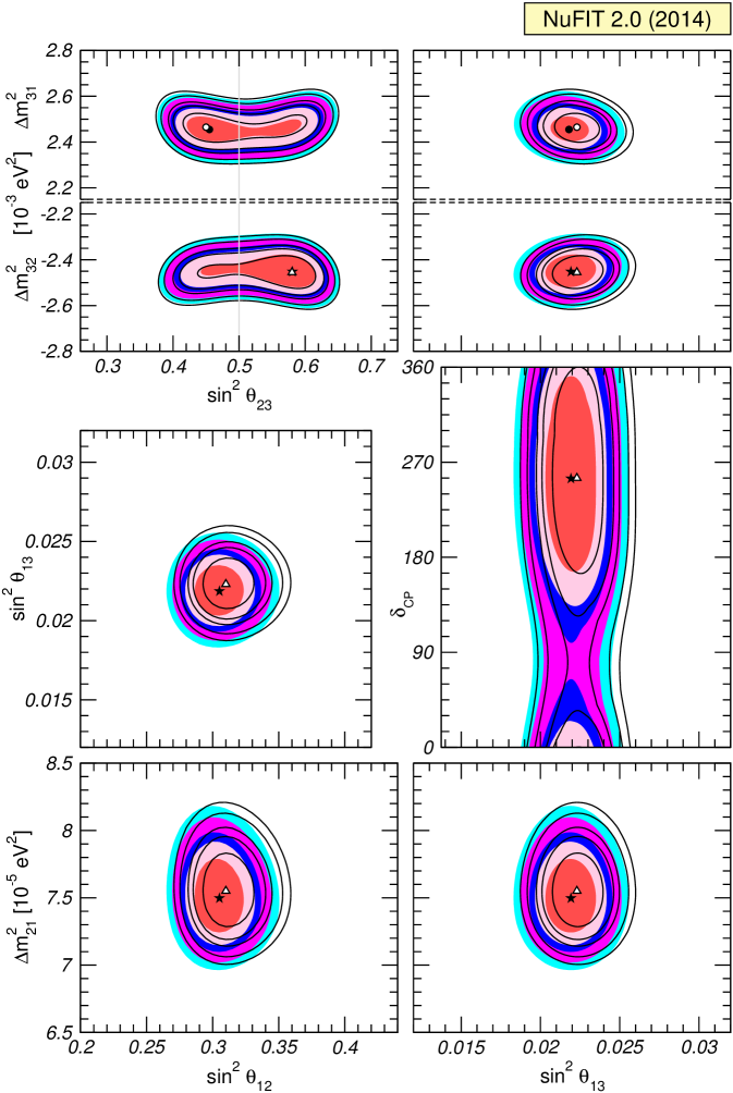
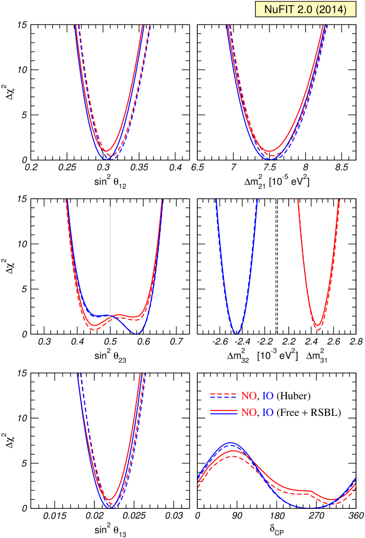
The results of the global analysis are presented in Figs. 1 and 2 where we show different projections of the allowed six-dimensional parameter space. To account for the possible effect of the so-called reactor anomaly Mueller:2011nm ; Huber:2011wv ; Mention:2011rk , we follow the approach of Refs. Schwetz:2011qt ; GonzalezGarcia:2012sz and study the dependence of the determined value of the parameters on the assumptions about the reactor fluxes. To bracket the possible impact of the anomaly, the results in Figs. 1 and 2 are shown for two extreme choices. The first option is to leave the normalization of reactor fluxes free and include data from short-baseline (less than 100 m) reactor experiments. This corresponds to the colored regions in Fig. 1 and the solid curves in Fig. 2 (labeled “Free+RSBL”). The second option is not to include short-baseline reactor data but assume reactor fluxes as predicted in Huber:2011wv (including their uncertainties). This corresponds to the black contours in Fig. 1 and the dashed curves in Fig. 2 (labeled “Huber”). From the results in these figures we conclude that:

1. for either choice of the reactor fluxes the global best fit corresponds to IO with $\sin^{2}\theta_{23}>0.5$, while the second local minima is for NO and with $\sin^{2}\theta_{23}<0.5$;

2. the statistical significance of the preference for Inverted versus Normal ordering is quite small, $\Delta\chi^{2}\lesssim 1\sigma$;

3. the present global analysis disfavors $\theta_{13}=0$ with a $\Delta\chi^{2}\approx 500$. Such impressive result is mostly driven by the reactor data from Daya Bay with secondary contributions from RENO and Double Chooz;

4. the uncertainty on $\theta_{13}$ associated with the choice of reactor fluxes is reduced to the level of $0.5\sigma$ in the global analysis. This is so because the most precise results from Daya Bay and RENO are reactor flux normalization independent, as further discussed in Sec. 4.1;

5. a non-maximal value of the $\theta_{23}$ mixing is slightly favored, at the level of $\sim 1.4\sigma$ for Inverted Ordering at of $\sim 1.0\sigma$ for Normal Ordering;

6. the statistical significance of the preference of the fit for the second (first) octant of $\theta_{23}$ is $\leq 1.4\sigma$ ($\leq 1.0\sigma$) for IO (NO);

7. the best fit for $\delta_{\text{CP}}$ for all analyses and orderings occurs for $\delta_{\text{CP}}\simeq 3\pi/2$, and values around $\pi/2$ are disfavored with $\Delta\chi^{2}\simeq 6$. A discussion on the corresponding CL can be found in Sec. 4.5.

	Normal Ordering ($\Delta\chi^{2}=0.97$)		Inverted Ordering (best fit)		Any Ordering
	bfp $\pm 1\sigma$	$3\sigma$ range	bfp $\pm 1\sigma$	$3\sigma$ range	$3\sigma$ range
$\sin^{2}\theta_{12}$	$0.304_{-0.012}^{+0.013}$	$0.270\to 0.344$	$0.304_{-0.012}^{+0.013}$	$0.270\to 0.344$	$0.270\to 0.344$
$\theta_{12}/^{\circ}$	$33.48_{-0.75}^{+0.78}$	$31.29\to 35.91$	$33.48_{-0.75}^{+0.78}$	$31.29\to 35.91$	$31.29\to 35.91$
$\sin^{2}\theta_{23}$	$0.452_{-0.028}^{+0.052}$	$0.382\to 0.643$	$0.579_{-0.037}^{+0.025}$	$0.389\to 0.644$	$0.385\to 0.644$
$\theta_{23}/^{\circ}$	$42.3_{-1.6}^{+3.0}$	$38.2\to 53.3$	$49.5_{-2.2}^{+1.5}$	$38.6\to 53.3$	$38.3\to 53.3$
$\sin^{2}\theta_{13}$	$0.0218_{-0.0010}^{+0.0010}$	$0.0186\to 0.0250$	$0.0219_{-0.0010}^{+0.0011}$	$0.0188\to 0.0251$	$0.0188\to 0.0251$
$\theta_{13}/^{\circ}$	$8.50_{-0.21}^{+0.20}$	$7.85\to 9.10$	$8.51_{-0.21}^{+0.20}$	$7.87\to 9.11$	$7.87\to 9.11$
$\delta_{\text{CP}}/^{\circ}$	$306_{-70}^{+39}$	$\hphantom{00}0\to 360$	$254_{-62}^{+63}$	$\hphantom{00}0\to 360$	$\hphantom{00}0\to 360$
$\dfrac{\Delta m^{2}_{21}}{10^{-5}~{}\text{eV}^{2}}$	$7.50_{-0.17}^{+0.19}$	$7.02\to 8.09$	$7.50_{-0.17}^{+0.19}$	$7.02\to 8.09$	$7.02\to 8.09$
$\dfrac{\Delta m^{2}_{3\ell}}{10^{-3}~{}\text{eV}^{2}}$	$+2.457_{-0.047}^{+0.047}$	$+2.317\to+2.607$	$-2.449_{-0.047}^{+0.048}$	$-2.590\to-2.307$	$\begin{bmatrix}+2.325\to+2.599\\[-2.0pt] -2.590\to-2.307\end{bmatrix}$

Table 1: Three-flavor oscillation parameters from our fit to global data after the NOW 2014 conference. The results are presented for the “Free Fluxes + RSBL” in which reactor fluxes have been left free in the fit and short baseline reactor data (RSBL) with $L\lesssim 100$ m are included. The numbers in the 1st (2nd) column are obtained assuming NO (IO), i.e., relative to the respective local minimum, whereas in the 3rd column we minimize also with respect to the ordering. Note that $\Delta m^{2}_{3\ell}\equiv\Delta m^{2}_{31}>0$ for NO and $\Delta m^{2}_{3\ell}\equiv\Delta m^{2}_{32}<0$ for IO.

In what follows we will consider our default analysis choice the one with “Free Fluxes + RSBL”. It is for this choice of fluxes that the best fit values and the derived ranges for the six parameters at the $1\sigma$ ($3\sigma$) level are given in Tab. 1. For each parameter the ranges are obtained after marginalizing with respect to the other parameters. We show the results for three scenarios. In the first and second columns we assume that the ordering of the neutrino mass states is known “a priori” to be Normal or Inverted, respectively, so the ranges of all parameters are defined with respect to the minimum in the given scenario. In the third column we make no assumptions on the ordering, so in this case the ranges of the parameters are defined with respect to the global minimum (which corresponds to Inverted Ordering) and are obtained marginalizing also over the ordering. For this third case we only give the $3\sigma$ ranges. Of course in this case the range of $\Delta m^{2}_{3\ell}$ is composed of two disconnected intervals, one one containing the absolute minimum (IO) and the other the secondary local minimum (NO).

Let us define the $3\sigma$ relative precision of a parameter by $2(x^{\text{up}}-x^{\text{low}})/(x^{\text{up}}+x^{\text{low}})$, where $x^{\text{up}}$ ($x^{\text{low}}$) is the upper (lower) bound on a parameter $x$ at the $3\sigma$ level. From the numbers in the table we then find $3\sigma$ relative precisions of 14% ($\theta_{12}$), 32% ($\theta_{23}$), 15% ($\theta_{13}$), 14% ($\Delta m^{2}_{21}$) and 11% ($|\Delta m^{2}_{3\ell}|$) for the various oscillation parameters.

3 Mixing matrix and leptonic CP violation

From the global $\chi^{2}$ analysis described in the previous section and following the procedure outlined in Ref. GonzalezGarcia:2003qf one can derive the $3\sigma$ ranges on the magnitude of the elements of the leptonic mixing matrix to be:

$$|U|=\begin{pmatrix}0.801\to 0.845&\qquad 0.514\to 0.580&\qquad 0.137\to 0.158\\ 0.225\to 0.517&\qquad 0.441\to 0.699&\qquad 0.614\to 0.793\\ 0.246\to 0.529&\qquad 0.464\to 0.713&\qquad 0.590\to 0.776\end{pmatrix}.$$ (4)

By construction the derived limits in Eq. (4) are obtained under the assumption of the matrix $U$ being unitary. In other words, the ranges in the different entries of the matrix are correlated due to the constraints imposed by unitarity, as well as the fact that, in general, the result of a given experiment restricts a combination of several entries of the matrix. As a consequence choosing a specific value for one element further restricts the range of the others.

Figure 3: Dependence of the global $\Delta\chi^{2}$ function on the Jarlskog invariant. The red (blue) curves are for NO (IO).

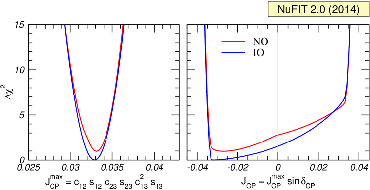
The present status of the determination of leptonic CP violation is illustrated in Fig. 3 where we show the dependence of the $\Delta\chi^{2}$ of the global analysis on the Jarlskog invariant which gives a convention-independent measure of CP violation Jarlskog:1985ht , defined as usual by:

$$\mathop{\rm Im}\big{[}U_{\alpha i}U_{\alpha j}^{*}U_{\beta i}^{*}U_{\beta j}\big{]}\equiv\sum_{\gamma=e,\mu,\tau}\sum_{k=1,2,3}\,J_{\text{CP}}\,\epsilon_{\alpha\beta\gamma}\,\epsilon_{ijk}\equiv J_{\text{CP}}^{\text{max}}\,\sin\delta_{\text{CP}}\,.$$ (5)

Using the parametrization in Eq. (1) we get

$$J^{\text{max}}_{\text{CP}}=\cos\theta_{12}\sin\theta_{12}\cos\theta_{23}\sin\theta_{23}\cos^{2}\theta_{13}\sin\theta_{13}\,.$$ (6)

From the left panel of Fig. 3 we see that the determination of the mixing angles yields at present a maximum allowed CP violation

$$J_{\text{CP}}^{\text{max}}=0.0329\pm 0.0009\;(\mathrel{\pm}0.0027)$$ (7)

at $1\sigma$ ($3\sigma$) for both orderings. The preference of the present data for non-zero $\delta_{\text{CP}}$ implies a best fit $J_{\text{CP}}^{\text{best}}=-0.032$, which is favored over CP conservation at the $\sim 1.2\sigma$ level. These numbers can be compared with the size of the Jarlskog invariant in the quark sector, which is determined to be $J_{\text{CP}}^{\text{quarks}}=(2.96^{+0.20}_{-0.16})\times 10^{-5}$ PDG .

Figure 4: Six leptonic unitarity triangles. After scaling and rotating each triangle so that two of its vertices always coincide with $(0,0)$ and $(1,0)$ (see text for details) we plot the $1\sigma$, 90%, $2\sigma$, 99%, $3\sigma$ CL (2 dof) allowed regions of the third vertex. Note that in the construction of the triangles the unitarity of the $U$ matrix is always explicitly imposed.

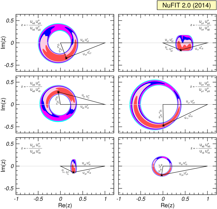
In Fig. 4 we recast the allowed regions for the leptonic mixing matrix in terms of leptonic unitarity triangles, which are obtained as different combinations of the entries of the $U$ matrix. Since in our analysis $U$ is unitary by construction, any given pair of rows or columns can be used to define a triangle in the complex plane. On the left (right) panels we show the triangles corresponding to the unitarity conditions

$$\sum_{i=1,2,3}U_{\alpha i}U^{*}_{\beta i} =0 \text{with~{}}\alpha\neq\beta$$ (left), (8)

$$\sum_{\alpha=e,\mu,\tau}U_{\alpha i}U^{*}_{\alpha j} =0 \text{with~{}}i\neq j$$ (right).

In drawing these triangles we have rescaled and rotated their sides so that two of their vertices always coincide with $(0,0)$ and $(1,0)$ in the complex plane. To this aim we have defined a complex variable $z$ as follows:

$$z=-\frac{U_{\alpha i}U^{*}_{\beta i}}{U_{\alpha k}U^{*}_{\beta k}} =1+\frac{U_{\alpha j}U^{*}_{\beta j}}{U_{\alpha k}U^{*}_{\beta k}} \text{with~{}}\alpha\neq\beta\text{~{}and~{}}i\neq j\neq k$$ (left), (9)

$$z=-\frac{U_{\alpha i}U^{*}_{\alpha j}}{U_{\gamma i}U^{*}_{\gamma j}} =1+\frac{U_{\beta i}U^{*}_{\beta j}}{U_{\gamma i}U^{*}_{\gamma j}} \text{with~{}}i\neq j\text{~{}and~{}}\alpha\neq\beta\neq\gamma$$ (right)

and then we have plot the $1\sigma$, 90%, $2\sigma$, 99%, $3\sigma$ CL (2 dof) allowed regions of the third vertex of the triangle as the real and imaginary parts of $z$. For convenience in each panel we have chosen the normalization side (the one which lies on the horizontal $(0,0)\to(0,1)$ segment) as the best determined of the two longer sides of each triangle. In this way all the triangles have more or less the same size, and the uncertainty in the position of the third vertex is not too much affected by the uncertainty of the normalization side. Note that the most common unitarity triangle in the quark sector is the one based on the $d$-quark and $b$-quark columns PDG , which corresponds to the 1st and 3rd column in the leptonic matrix, i.e., to the triangle in the middle-right panel in Fig. 4.

In this kind of diagrams the absence of CP violation implies a flat triangle, i.e., $\mathop{\rm Im}(z)=0$. As can be seen, in all the panels the horizontal axis marginally crosses the $1\sigma$ allowed region, which for 2 dof corresponds to $\Delta\chi^{2}\simeq 2.3$. This is consistent with the present preference for CP violation, $\chi^{2}(J_{\text{CP}}=0)-\chi^{2}(J_{\text{CP}}~{}\text{free})=1.5$.

4 Tension and tendencies

4.1 Impact of reactor flux uncertainties

Figure 5: Contours ($1\sigma$, 90%, $2\sigma$, 99%, $3\sigma$ CL for 2 dof) in the plane of $\theta_{13}$ and the reactor flux normalization $f_{\text{flux}}$. Full regions correspond to the combined analysis of all reactor neutrino experiments with the exception of KamLAND, but including the RSBL experiments. The green contours correspond to only the RSBL experiments and red contours include RSBL + medium-baseline reactors without a near detector (i.e. without including Daya Bay and RENO).

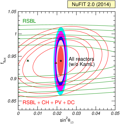
Within the 3-flavor framework the so-called reactor anomaly leads to a “tension” of about $2.7\sigma$ between the predicted reactor neutrino fluxes Mueller:2011nm ; Huber:2011wv and the event rates observed in short-baseline reactor experiments. By adopting two extreme approaches in dealing with this tension we have shown in Sec. 2.2 that the impact on the determination of the oscillation parameters in the global fit is quite small, at the level of $0.5\sigma$ for $\sin^{2}\theta_{13}$ (see Figs. 1 and 2). This is further illustrated in Fig. 5 where we show the allowed regions in the plane of $\theta_{13}$ and the flux normalization $f_{\text{flux}}$ (relative to the one predicted in Huber:2011wv ) for several combinations of the reactor experiments. Short-baseline data (green contours) essentially determine the flux normalization. Adding also data from experiments at around 1 km without a dedicated near detector (red contours) provides already a signal for non-zero $\theta_{13}$, but such result is affected by significant correlation with the flux normalization. However, once the precise data on near-far comparison from Daya Bay and RENO are included (colored regions) no correlation is left between the determination of $\theta_{13}$ and $f_{\text{flux}}$. Thus in the $3\nu$ analysis the unexplained reactor anomaly mostly translates in an overall increase of the $\chi^{2}$ in the analysis with fluxes from Ref. Huber:2011wv with $\chi^{2}(f_{\text{flux}}=1)-\chi^{2}(f_{\text{flux}}~{}\text{free})\simeq 7$. Details of our analysis in this respect can be found in Ref. Kopp:2013vaa , where a discussion of a possible explanation in terms of sterile neutrinos is also given.

4.2 Determination of $\Delta m^{2}_{21}$: solar and KamLAND

Figure 6: Left: Allowed parameter regions (at $1\sigma$, 90%, $2\sigma$, 99% and $3\sigma$ CL for 2 dof) from the combined analysis of solar data for GS98 model (full regions with best fit marked by black star) and AGSS09 model (dashed void contours with best fit marked by a white dot), and for the analysis of KamLAND data (solid green contours with best fit marked by a green star) for fixed $\theta_{13}=8.5^{\circ}$. We also show as orange contours the results of a global analysis for the GS98 model but without including the day-night information from SK (see text for details). Right: $\Delta\chi^{2}$ dependence on $\Delta m^{2}_{21}$ for the same four analysis after marginalizing over $\theta_{12}$.

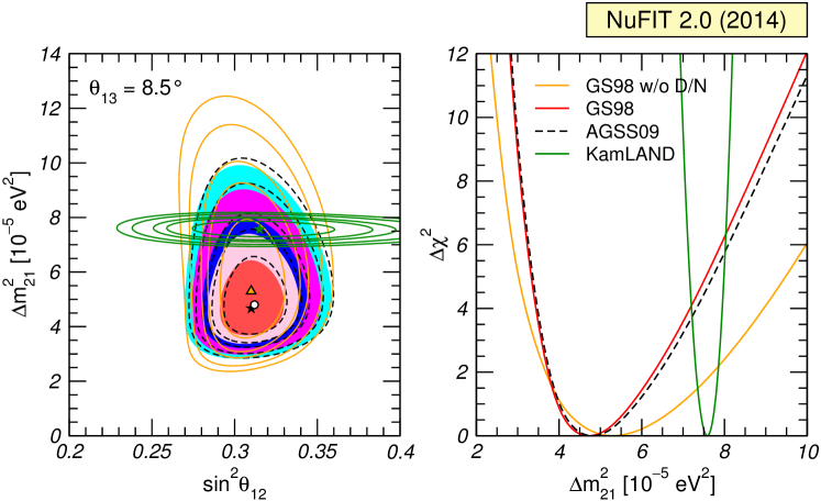
We show in Fig. 6 the results of the analysis of the solar experiments and of KamLAND which give the dominant contribution to the determination of $\Delta m^{2}_{21}$ and $\theta_{12}$. Here $\theta_{13}$ is fixed to the present best fit value of the global analysis. For the sake of completeness the solar neutrino results are shown for two different versions of the Standard Solar Model, namely the GS98 and the AGSS09 models Serenelli:2009yc . Let us remind that GS98 is based on the older solar abundances leading to high metallicity and which perfectly agreed with helioseismological data, whereas AGSS09 uses the new precise determination of the solar abundances which imply a lower metallicity and cannot reproduce the helioseismological data. This conflict constitutes the so-called “solar composition problem”. Although it is a pretty serious problem in the context of solar physics, its impact in the determination of the relevant oscillation parameters is very small, as can be seen clearly from Fig. 6.

The left panel in Fig. 6 illustrates the complementarity of solar and KamLAND in the determination of the “12” parameters. Solar experiments provide the best precision of $\theta_{12}$ while KamLAND gives a better determination of $\Delta m^{2}_{21}$. We remind the reader that the relevant survival probabilities for these experiments in the framework of three neutrino oscillations can be written as:

$$P^{3\nu}_{ee}=\sin^{4}\theta_{13}+\cos^{4}\theta_{13}P^{2\nu}_{ee}(\Delta m^{2}_{21},\theta_{12})\,,$$ (10)

where we have used the fact that $L^{\text{osc}}_{31}=4\pi E_{\nu}/\Delta m^{2}_{31}$ is much shorter than the distance traveled by both solar and KamLAND neutrinos, so that the oscillations related to ${L_{31}^{\text{osc}}}$ are averaged. In presence of matter effects $P^{2\nu}_{ee}(\Delta m^{2}_{21},\theta_{12})$ should be calculated taking into account the evolution in an effective matter density $n^{\text{eff}}_{e}=n_{e}\cos^{2}\theta_{13}$. For $10^{-5}\lesssim\Delta m^{2}/\text{eV}^{2}\lesssim 10^{-4}$, $P^{2\nu}_{ee}(\Delta m^{2}_{21},\theta_{12})$ presents the following asymptotic behaviors Goswami:2004cn :

$$P^{2\nu,\text{sun}}_{ee} \simeq 1-\frac{1}{2}\sin^{2}(2\theta_{12}) \text{for~{}}E_{\nu} \lesssim\text{few}\times 100~{}\text{KeV}$$ (11)

$$P^{2\nu,\text{sun}}_{ee} \simeq\sin^{2}(\theta_{12}) \text{for~{}}E_{\nu} \gtrsim\text{few}\times 1~{}\text{MeV}$$ (12)

$$P_{ee}^{2\nu,\text{kam}} =1-\frac{1}{2}\sin^{2}(2\theta_{12})\sin^{2}\frac{\Delta m^{2}_{21}L}{2E_{\nu}}\,.$$ (13)

At present most of the precision of the solar analysis is provided by SNO and SK for which the relevant MSW survival probability Wolfenstein:1977ue ; Mikheev:1986gs provides a direct measurement of $\sin^{2}\theta_{12}$, as seen in Eq. (12). In the MSW regime the determination of $\Delta m^{2}_{21}$ in solar experiments comes dominantly from the ratio between the solar potential and the $\Delta m^{2}_{21}$ term required to simultaneously describe the CC/NC data at SNO and the undistorted spectra of $\mbox{}^{8}\text{B}$ neutrinos as measured in both SK and SNO. Conversely KamLAND $\bar{\nu}_{e}$ survival probability proceeds dominantly as vacuum oscillations and provides a most precise determination of $\Delta m^{2}_{21}$ via the strong effect of the oscillating phase in the distortion of the reactor energy spectrum. On the contrary it yields a weaker constraint on $\theta_{12}$ as the vacuum oscillation probability depends on the double-valued and “flatter” function $\sin^{2}(2\theta_{12})$.

As seen in the left panel in Fig. 6 for either version of the solar model the best fit points of solar and KamLAND analysis lie at very similar values of $\theta_{12}$. As it was pointed out in Ref. Fogli:2008jx and widely discussed in the literature Fogli:2009zza ; Schwetz:2008er ; Maltoni:2008ka ; Balantekin:2008zm ; GonzalezGarcia:2010er , the matching in the determination of $\theta_{12}$ requires the presence of a non-zero value of $\theta_{13}$. With the present determination of $\theta_{13}$ provided by the medium baseline reactor experiments, the agreement between the best fit point values of $\theta_{12}$ is remarkable.

From the same figure, however, we see that the value of $\Delta m^{2}_{21}$ preferred by KamLAND is higher than the one from solar experiments. At present this is about a $2\sigma$ effect, as can be seen in the right panel where we show the $\Delta\chi^{2}$ dependence as a function of $\Delta m^{2}_{21}$ when marginalized over $\theta_{12}$. This tension has been present during the last two years and it arises from a combination of two effects: (a) the well-known fact that none of the $\mbox{}^{8}\text{B}$ measurement performed by SNO, SK and Borexino show any evidence of the spectrum low energy turn-up expected in the standard LMA-MSW solution, and (b) the indication of a non-vanishing day-night asymmetry in SK, which disfavors the KamLAND $\Delta m^{2}_{21}$ best fit value for which Earth matter effects are too small. The relevance of these effects is illustrated in Fig. 6 where we show the results of our analysis both with and without the inclusion of the SK day-night information. As can be seen, once the SK day-night information is removed the solar best-fit point shifts upwards and the solar allowed region extends to much larger values of $\Delta m^{2}_{21}$, as expected, so that the tension with KamLAND is reduced to about $1.4\sigma$. Modified matter potential due to non-standard interactions Palazzo:2011vg ; Gonzalez-Garcia:2013usa and super-light sterile neutrinos deHolanda:2010am have been proposed as extended scenarios which could relax this tension.

4.3 Determination of $\Delta m^{2}_{3\ell}$: $\nu_{\mu}$ and $\nu_{e}$ disappearance

Figure 7: Determination of $\Delta m^{2}_{3\ell}$ at $1\sigma$ and $2\sigma$ (2 dof), where $\ell=1$ for NO (upper panels) and $\ell=2$ for IO (lower panels). The left panels show regions in the $(\sin^{2}\theta_{23},\Delta m^{2}_{3\ell})$ plane using both appearance and disappearance data from MINOS (green) and T2K (black), as well as SK atmospheric data (green) and a combination of them (colored regions). Here $\theta_{13}$ is constrained to the $3\sigma$ range from the global fit. The right panels show regions in the $(\sin^{2}\theta_{13},\Delta m^{2}_{3\ell})$ plane using data from Daya Bay (black), reactor data without Daya Bay (violet), and their combination (colored regions). In all panels solar and KamLAND data are included to constrain $\Delta m^{2}_{21}$ and $\theta_{12}$. Contours are defined with respect to the local minimum in each panel.

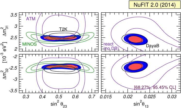
Fig. 7 illustrates the determination of $\Delta m^{2}_{3\ell}$ from different data sets. In the left panels we focus on long-baseline $\nu_{\mu}$ disappearance data. It is clear that in this case the final precision on $|\Delta m^{2}_{3\ell}|$ emerges from the combination of T2K and MINOS data, while the determination of $\sin^{2}\theta_{23}$ is dominated by T2K.

Concerning $\nu_{e}$ disappearance data, Eq. (17) in Sec. 4.4 implies that the rates observed in reactor experiments at different baselines can provide an independent determination of $\Delta m^{2}_{3\ell}$ Bezerra:2012at ; GonzalezGarcia:2012sz . On top of this, the observation of the energy-dependent oscillation effect of $\theta_{13}$ in Daya Bay An:2013zwz allows a rather precise determination of $|\Delta m^{2}_{3\ell}|$. In the right panels of Fig. 7 we show therefore the allowed regions in the $(\theta_{13},\Delta m^{2}_{3\ell})$ plane based on global data on $\nu_{e}$ disappearance. The blue contours are obtained from all the medium-baselines reactor experiments with the exception of Daya Bay. Those regions emerge from the baseline effect mentioned above. The black contour are based on the energy spectrum in Daya Bay, whereas the colored regions show the combination.

By comparing the left and right panels we observe that $\nu_{\mu}$ and $\nu_{e}$ disappearance experiments by now provide a consistent determination of $|\Delta m^{2}_{3\ell}|$ with similar precision.

4.4 Mass ordering, $\theta_{23}$ octant and CP phase: role of different data sets

As we have seen in Sec. 2, several 1-2$\sigma$ “tendencies” appear in the global analysis in the determination of the mass ordering, the octant of $\theta_{23}$, and the CP violating phase. To illustrate the role of the different data sets on such tendencies, we show in Fig. 8 the $\Delta\chi^{2}$ as a function of $\Delta m^{2}_{3\ell}$, $\theta_{23}$, and $\delta_{\text{CP}}$ for different combinations of experiments. In each panel the results have been marginalized with respect to all undisplayed parameters except the mass ordering, which is fixed to Inverted (Normal) for the left (right) panels. Note, however, that for each combination of experiments the $\Delta\chi^{2}$ is defined with respect to the absolute minima between the two orderings. In this way the difference between the “height” of the minimum of the curve on the left and the corresponding one on the right gives the contribution of that set of observables to the determination of the mass ordering.

Figure 8: Contribution of different sets of experimental results to the present tendencies in the determination of the mass ordering, the octant of $\theta_{23}$ and of the CP violating phase. Left (right) panels are for IO (NO). See text for details.

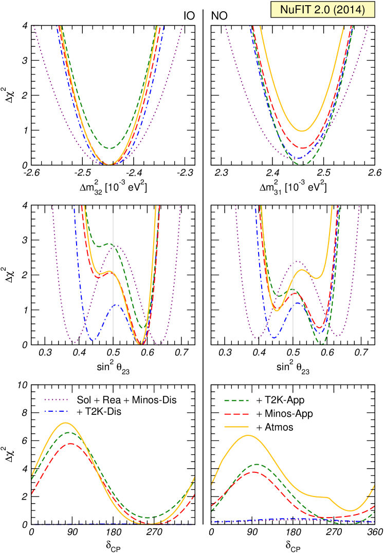
All the lines plotted in Fig. 8 include “by default” solar and reactor data, which take care of precisely determining the undisplayed parameters $\Delta m^{2}_{21}$, $\theta_{12}$ and $\theta_{13}$. To this basic set we progressively add more and more data, to see how each new piece of information affects the results of the fit. Let us then start with the dotted purple (and dot-dashed blue) curve, which shows the dependence of $\Delta\chi^{2}$ on the analysis of solar, reactor and MINOS (plus T2K) $\nu_{\mu}$ and $\bar{\nu}_{\mu}$ disappearance data. Being all disappearance experiments they provide very weak information on $\delta_{\text{CP}}$, as clearly visible in the bottom panels. Comparing the minima in the left and right panels we note a relative difference of $\chi^{2}(\text{NO})-\chi^{2}(\text{IO})\sim 0.2$, which means that this combination of data “favors” Inverted Ordering by $\sim 0.5\sigma$. More interestingly, from the central panels we see that MINOS disappearance data favors a non-maximal $\theta_{23}$ with $\Delta\chi^{2}(\theta_{23}=45^{\circ})=2.8$ ($2.2$) for IO (NO). Neglecting subleading $\Delta m^{2}_{21}$ and matter effects, the relevant survival probability in MINOS is given by

$$P_{\nu_{\mu}\to\nu_{\mu}}\approx 1-\sin^{2}2\theta_{\text{dis}}\,\sin^{2}\frac{\Delta m^{2}_{31}L}{4E_{\nu}}\,,\qquad\sin^{2}\theta_{\text{dis}}\equiv\sin^{2}\theta_{23}\cos^{2}\theta_{13}\,,$$ (14)

where $L$ is the baseline and $E_{\nu}$ is the neutrino energy. Hence, the probability is symmetric under $\theta_{\text{dis}}\to\pi/2-\theta_{\text{dis}}$. In the limit $\theta_{13}=0$ the effective angle $\theta_{\text{dis}}$ reduces to $\theta_{23}$, and a preference for non-maximal $\theta_{\text{dis}}$ mixing leads to the appearance of two symmetric minima in the first and second octant of $\theta_{23}$. Such degeneracy persists also for $\theta_{13}\neq 0$, and is responsible for the presence of two quasi-degenerate minima at $\sin^{2}\theta_{23}=0.63$ and $0.39$. On the other hand, T2K disappearance data are better fitted with maximal $\theta_{\text{dis}}$, so once they are included in the analysis (dot-dashed blue line) the positions of the two minima move to values $\sin^{2}\theta_{23}=0.58$ and $0.44$ while the preference for non-maximal mixing reduces to $\Delta\chi^{2}(\theta_{23}=45^{\circ})=1$. The comparison of the dotted purple and dot-dashed blue curves also shows the impact of the inclusion of T2K disappearance data on the overall determination of $\theta_{23}$ and $\Delta m^{2}_{3\ell}$.

The short-dashed green line shows the effect of further adding to the analysis the T2K $\nu_{e}$ appearance data. First, we see that the absolute minima now occurs for NO with $\Delta\chi^{2}(\text{IO})=0.6$. In the central panels we see that the quasi-degeneracy of the octant of $\theta_{23}$ is now broken and the second octant becomes favored with $\Delta\chi^{2}(\theta_{23}\leq 45^{\circ})=2.5$ ($1.5$) for IO (NO). The lower panels show that after the inclusion of T2K $\nu_{e}$ appearance data a minimum appears for $\delta_{\text{CP}}=270^{\circ}$ ($300^{\circ}$) for IO (NO) with CP conservation disfavored at $\Delta\chi^{2}(\sin\delta_{\text{CP}}=0)=2.5$ ($1.0$). This can be understood from the relevant $\nu_{e}$ appearance probability at T2K and MINOS, which, at the second order in the small parameters $\sin\theta_{13}$ and $\alpha\equiv\Delta m^{2}_{21}/\Delta m^{2}_{31}$ and assuming a constant matter density, takes the form Cervera:2000kp ; Freund:2001pn ; Akhmedov:2004ny :

$$P_{\nu_{\mu}\to\nu_{e}}\approx 4\,\sin^{2}\theta_{13}\,\sin^{2}\theta_{23}\frac{\sin^{2}\Delta(1-A)}{(1-A)^{2}}+\alpha^{2}\sin^{2}2\theta_{12}\,\cos^{2}\theta_{23}\frac{\sin^{2}A\Delta}{A^{2}}\\ +2\,\alpha\,\sin\theta_{13}\,\sin 2\theta_{12}\,\sin 2\theta_{23}\cos(\Delta\pm\delta_{\text{CP}})\,\frac{\sin\Delta A}{A}\,\frac{\sin\Delta(1-A)}{1-A}\,,$$ (15)

with

$$\Delta\equiv\frac{\Delta m^{2}_{31}L}{4E_{\nu}}\,,\quad A\equiv\frac{2E_{\nu}V}{\Delta m^{2}_{31}}\,.$$ (16)

Here $L$ is the baseline, $E_{\nu}$ is the neutrino energy, and $V$ is the effective matter potential Wolfenstein:1977ue which for T2K yields $|A|\sim\text{few}~{}\%$. The first term in Eq. (15) (which dominates for large $\theta_{13}$) depends on $\sin^{2}\theta_{23}$ and therefore is sensitive to the octant. Reactor experiments with $L\sim 1$ km, on the other hand, provide a measurement of $\theta_{13}$ independent of $\theta_{23}$

$$P_{\nu_{e}\to\nu_{e}}=1-\sin^{2}2\theta_{13}\sin^{2}\frac{\Delta m^{2}_{31}L}{4E_{\nu}}+\mathcal{O}(\alpha^{2})\,.$$ (17)

At present the $\nu_{e}$ appearance results from T2K points towards an excess with respect to what is expected for the best fit value of $\sin^{2}\theta_{13}$ determined by the reactor experiments for maximal $\theta_{23}$ (i.e., for $2\sin^{2}\theta_{23}=1$), hence the tendency towards the $\theta_{23}>45^{\circ}$ minimum. The matter effects in Eq. (15) make this tendency different for NO and IO, while the last term introduces a $\delta_{\text{CP}}$ modulation of the effect. For fixed $\theta_{13}$ and $\theta_{23}$, $P_{\nu_{\mu}\to\nu_{e}}(\delta_{\text{CP}})-P_{\nu_{\mu}\to\nu_{e}}(\pi)\geq 0$ ($\leq 0$) for $\delta_{\text{CP}}\geq\pi$ ($\leq\pi$). For the best fit values of $\theta_{13}$ and $\theta_{23}$ from the previous reactor and LBL $\nu_{\mu}$ disappearance results, the T2K $\nu_{e}$ appearance signal is better fitted with $\delta_{\text{CP}}$ values which enhance the corresponding appearance probability. Conversely we see that adding the less significant MINOS $\nu_{e}$ appearance data in the analysis (long-dashed red curves) tends to slightly reduce the size of these effects for NO and it shifts the global minimum from NO to IO.

Finally the solid orange curves show the impact of including the atmospheric data in the analysis. Comparing the solid orange and long-dashed red curves we see that atmospheric data contributes positively to the significance of the tendency towards IO and $\delta_{\text{CP}}>\pi$. While for IO it does not affect the tendency towards second $\theta_{23}$ octant, for NO it “shifts” this tendency to the first octant. The preference for $\theta_{23}<45^{\circ}$ for NO is related to an excess of sub-GeV e-like events, an effect which has already been discussed since many years (see, e.g., Kim:1998bv ; Peres:1999yi ; Peres:2003wd ; Gonzalez-Garcia:2004cu ). The fact that this preference is not visible for IO is probably related to multi-GeV data, which are affected by matter effects and therefore provides some sensitivity to the mass ordering. Identifying the relevant bins is difficult, given the large amount of data points entering the atmospheric fit. We stress that such effects happen at the level of 1-2 units in $\chi^{2}$ and hence are not statistically significant.

Figure 9: Allowed regions from the global data at $1\sigma$, 90%, $2\sigma$, 99% and $3\sigma$ CL (2 dof) in the $(\theta_{23},\delta_{\text{CP}})$ plane, after minimizing with respect to all undisplayed parameters. The left (right) panel corresponds to IO (NO). Contour regions in both panels are derived with respect to the global minimum which occurs for IO and is indicated by a star. The local minimum for NO is shown by a black dot.

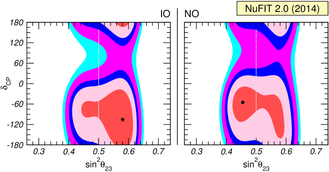
In order to highlight the pattern of correlations between $\delta_{\text{CP}}$ and $\sin^{2}\theta_{23}$ we show in Fig. 9 the allowed regions of the global analysis projected into the plane of these two parameters. Correlations between $\delta_{\text{CP}}$ and other oscillation parameters are mostly trivial and are therefore omitted.

4.5 Remarks on confidence levels for $\delta_{\text{CP}}$

In order to study the information from data on the CP phase we consider the quantity

$$\Delta\chi^{2}(\delta_{\text{CP}})\equiv\min_{x\neq\delta_{\text{CP}}}\chi^{2}(\delta_{\text{CP}},x)-\chi^{2}_{\text{min}}\,,$$ (18)

where the first term on the right hand side is minimized with respect to all oscillation parameters except $\delta_{\text{CP}}$ ($x=\theta_{12},\theta_{13},\theta_{23},\Delta m^{2}_{21},\Delta m^{2}_{31}$) and the last term is the $\chi^{2}$ minimum with respect to all oscillation parameters. We have shown $\Delta\chi^{2}(\delta_{\text{CP}})$ for various data sets in the lower panels of Fig. 8, as well as in the corresponding panel in Fig. 2 for the global data. The standard way to derive confidence intervals for $\delta_{\text{CP}}$ is to assume that $\Delta\chi^{2}(\delta_{\text{CP}})$ follows a $\chi^{2}$-distribution with 1 dof, and then apply cuts corresponding to, e.g., $\Delta\chi^{2}=0.99$, $2.71$, $3.84$, $6.63$ for 68%, 90%, 95%, 99% CL, respectively. This procedure relies on Wilks theorem to hold Wilks . However, in the case of $\delta_{\text{CP}}$ some of the hypothesis of this theorem may be violated Schwetz:2006md ; Blennow:2014sja . One reason for this is the complicated non-linear dependence of the event rates on $\delta_{\text{CP}}$. Present sensitivity is so poor, that those non-linearities (as well as the periodic character of $\delta_{\text{CP}}$) become relevant already at very low CL. Furthermore, parameter degeneracies (especially with $\theta_{23}$, see discussion in the previous sub-section) affect the distribution of the test statistic $\Delta\chi^{2}$ from Eq. (18).

Figure 10: Black curves show the $\Delta\chi^{2}$ levels corresponding to 68%, 90%, 95%, 99% CL obtained from a Monte Carlo simulation of T2K appearance and disappearance data. Dashed lines correspond to the canonical values based on the $\chi^{2}$ distribution with 1 dof. The blue curve shows the observed $\Delta\chi^{2}$ using T2K data. The shaded regions indicate the 90% confidence interval for $\delta_{\text{CP}}$ based on the distribution from simulated pseudo-data (brown) and on the $\chi^{2}$ approximation (gray). The three panels correspond to different assumptions on the true value of $\theta_{23}$ used to generate the pseudo-data. In the fit all parameters except $\delta_{\text{CP}}$ and $\theta_{23}$ are fixed to the global best fit values, assuming normal mass ordering.

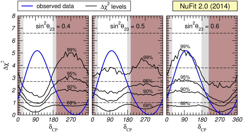
In order to address such concerns we have performed a Monte Carlo study of T2K data (appearance and disappearance). We consider a test statistic similar to the $\Delta\chi^{2}$ given in Eq. (18); however, in order to keep calculation time manageable we fix all oscillation parameters except $\delta_{\text{CP}}$ and $\theta_{23}$ to their best fit values from the global fit assuming normal mass ordering. Hence, in the notation of Eq. (18) we have only $x=\theta_{23}$. In particular, since we keep also $\theta_{13}$ fixed, the main feature of the complementarity of long-baseline appearance and medium-baseline reactor data is maintained. We have checked that allowing $\theta_{13}$ to vary imposing the constraint from Daya Bay data has a negligible impact on $\Delta\chi^{2}(\delta_{\text{CP}})$ compared to fixing it to the best fit value. The resulting $\Delta\chi^{2}(\delta_{\text{CP}})$ is shown as blue curve in Fig. 10 (identical in all three panels). It differs somewhat from the global result displayed in Figs. 2 or 8, which include more data, but it captures the essential features and suffices for the purpose of studying the statistical properties of the test statistic.

In order to estimate the probability distribution for $\Delta\chi^{2}(\delta_{\text{CP}})$ we proceed as follows. We scan the parameter space of $\delta_{\text{CP}}$ and $\sin^{2}\theta_{23}$ and for a given point of assumed true values we generate a large number of pseudo-data samples for T2K. For each data set we calculate the value of the test statistic $\Delta\chi^{2}(\delta_{\text{CP}})$ and in this way we obtain a distribution for it. We scan 41 points in $\delta_{\text{CP}}$ and 3 points for $\sin^{2}\theta_{23}$, and for each of those points we generate 5000 pseudo-data samples. The black curves in Fig. 10 show the values of $\Delta\chi^{2}(\delta_{\text{CP}})$ which are larger than 68%, 90%, 95% and 99% of all generated data samples. We observe quite large deviations from the corresponding values based on the $\chi^{2}$-distribution for 1 dof, shown by the dashed lines in the figure. Interestingly we find also a rather strong dependence on the assumed true value of $\theta_{23}$.

The behavior of the curves can be understood qualitatively. Due to the non-linearity of $\delta_{\text{CP}}$ (its cyclic nature) and the poor sensitivity mentioned above it actually counts as less than 1 full degree of freedom, which implies distributions more concentrated at lower values than the $\chi^{2}$-distribution for 1 dof, as observed in Fig. 10. The rather strong variations for non-maximal values of $\theta_{23}$, including a flipped behavior for $\delta_{\text{CP}}$ smaller or larger $\pi$ between $\sin^{2}\theta_{23}=0.4$ and $0.6$ can be understood in terms of a degeneracy. For $\theta_{23}<\pi/4$ and $\delta_{\text{CP}}\sim 3\pi/2$ as well as for for $\theta_{23}>\pi/4$ and $\delta_{\text{CP}}\sim\pi/2$ there is a degeneracy between the two octants of $\theta_{23}$ which effectively enhances the number of degrees of freedom in the fit.

Now we can compare $\Delta\chi^{2}(\delta_{\text{CP}})$ obtained from the observed data to the expected distribution. If the observed $\Delta\chi^{2}(\delta_{\text{CP}})$ is larger than the values obtained for $x\%$ of the pseudo-data samples for that true value of $\delta_{\text{CP}}$ we exclude this value of $\delta_{\text{CP}}$ at the $x\%$ CL. In Fig. 10 we show as an example the resulting 90% confidence interval for $\delta_{\text{CP}}$ as brown shaded area. This corresponds to the confidence interval according to the Feldman-Cousins (FC) prescription Feldman:1997qc . It has to be compared to the corresponding interval based on the $\chi^{2}$-approximation, indicated by the gray area in the plot.

We can draw the following conclusions from the exercise shown in Fig. 10:

1. the confidence intervals based on the Monte Carlo simulation are smaller than the ones based on the $\chi^{2}$-approximation. Hence, the latter is conservative;

2. for confidence levels $\lesssim 90\%$ the confidence intervals are similar, whereas for higher confidence levels differences become significant. In particular, at 99% CL all values of $\delta_{\text{CP}}$ are allowed using the $\chi^{2}$-approximation, whereas a region around $\delta_{\text{CP}}\sim\pi/2$ remains excluded by the 99% CL FC interval;

3. the CL with which $\delta_{\text{CP}}\sim\pi/2$ can be disfavored depends strongly on the unknown true value of $\theta_{23}$. For $\sin^{2}\theta_{23}=0.6$, $\delta_{\text{CP}}\simeq\pi/2$ is excluded at about 99% CL, whereas for $\sin^{2}\theta_{23}=0.4$ it is excluded at very high CL. In all cases, the CL based on the Monte Carlo is higher than in the $\chi^{2}$-approximation which again can be considered conservative.

Let us conclude this section by commenting that ideally such a simulation should be performed also for the global analysis. Unfortunately this is currently out of question, in particular due to atmospheric neutrino data, which is very computational intensive and does play a non-negligible role in the global fit for $\Delta\chi^{2}(\delta_{\text{CP}})$, see Fig. 8. However, we believe that the above results based on T2K are approximately representative also for the global fit. One may expect that, with more statistics, distributions become more close to the expected $\chi^{2}$-distribution. However, preliminary estimates indicate that parameter degeneracies may lead to deviations also in a high-statistics scenario.

5 Summary

We have presented the results of an updated (as of summer 2014) global analysis of solar, atmospheric, reactor and accelerator neutrino data in the framework of three-neutrino oscillations. Quantitatively the present determination of the oscillation parameters is listed in Table 1, and the corresponding leptonic mixing matrix is given in Eq. (4). From the present analysis we have derived the maximum allowed CP violation in the leptonic sector as parametrized by the Jarlskog determinant, $J_{\text{CP}}^{\text{max}}=0.0329\pm 0.0009$ ($\mathrel{\pm}0.0027$) at $1\sigma$ ($3\sigma$). All these results have also been shown in terms of unitarity triangles in Fig. 4 which further illustrate the ability of global oscillation data to obtain information on leptonic CP violation.

The global analysis presents a series of tensions between data sets as well as some 1-2$\sigma$ effects in the determination of less known parameters ($\theta_{23}$, mass ordering, and $\delta_{\text{CP}}$) which we denote as “tendencies” and we discuss in Sec. 4. We can summarize these results as follows:

• due to the very precise determination of the flux-independent near-far ratio from Daya Bay and RENO, the so-called reactor neutrino anomaly (i.e., the tension between the predicted reactor fluxes in Refs. Mueller:2011nm ; Huber:2011wv and the event rates observed in short-baseline reactor experiments) results only in a $0.5\sigma$ uncertainty on the determination of $\theta_{13}$;

• the long-standing $\sim 2\sigma$ tension between the best fit values of $\Delta m^{2}_{21}$ as determined from the analysis of KamLAND and solar data is still unresolved. This tension is driven by both the indication of a non-zero day-night effect at SK, and by the lack of evidence of a low energy turn-up in the $\mbox{}^{8}\text{B}$ energy spectrum as measured by SNO, SK4 and Borexino. In both cases the $\Delta m^{2}_{21}$ value favored by KamLAND is in disagreement with the expectations from the standard LMA-MSW solution;

• the uncertainty on the determination of $\Delta m^{2}_{21}$ and $\theta_{12}$ due to the choice of Standard Solar Model associated with the “solar composition problem” is negligible;

• at present the precision on the determination of $|\Delta m^{2}_{3\ell}|$ from $\nu_{\mu}$ disappearance experiments (mainly T2K and MINOS) is comparable to that from $\nu_{e}$ disappearance experiments (i.e. reactor experiments including, in particular, the spectral information from Daya Bay);

• for Inverted Ordering, the “tendency” towards non-maximal mixing and second octant of $\theta_{23}$ is driven mainly by two effects: (a) the non-maximality favored by MINOS $\nu_{\mu}$ disappearance, and (b) the “mismatch” between the best fit $\theta_{13}$ obtained from $\bar{\nu}_{e}$ disappearance at reactors and from $\nu_{\mu}\to\nu_{e}$ at T2K. Atmospheric results do not alter this;

• for Normal Ordering, such preference for non-maximal $\theta_{23}$ mixing is considerably weaker than for IO; also, in this case the global best-fit occur in the first $\theta_{23}$ octant, mostly driven by atmospheric data;

• the “mismatch” between reactor and T2K results is the driving effect in the present dependence of the global $\Delta\chi^{2}$ on the CP violating phase with a best fit value close to $\delta_{\text{CP}}=\frac{3}{2}\pi$. Inclusion of the atmospheric results adds positively to this effect for both orderings;

• the tendency towards IO or NO in the present analysis does not seem to result from any consistent effect and it shifts in sign depending on the data sets considered.

Finally in Sec. 4.5 we have addressed the issue of the “gaussianity” of the confidence levels attributed to $\Delta\chi^{2}(\delta_{\text{CP}})$ by performing a Monte Carlo study of T2K data, and we have compared the resulting probability distribution to that of a $\chi^{2}$-distribution as usually assumed. Deviations are expected due to the cyclic nature of $\delta_{\text{CP}}$ and to the presence of parameter degeneracies. The conclusion is that, within the present data, the use of the $\chi^{2}$-distribution approximation is slightly conservative in the determination of the excluded range of $\delta_{\text{C}P}$ at confidence levels $\gtrsim 90\%$. The differences however are not very significant as illustrated in Fig. 10.

Future updates of this analysis will be provided at the website quoted in Ref. nufit .

Appendix A List of data used in the analysis

Solar experiments

• Chlorine total rate Cleveland:1998nv , 1 data point.

• Gallex & GNO total rates Kaether:2010ag , 2 data points.

• SAGE total rate Abdurashitov:2009tn , 1 data point.

• SK1 full energy and zenith spectrum Hosaka:2005um , 44 data points.

• SK2 full energy and day/night spectrum Cravens:2008aa , 33 data points.

• SK3 full energy and day/night spectrum Abe:2010hy , 42 data points.

• SK4 1669-day energy spectrum and day/night asymmetry sksol:nu2014 , 24 data points.

• SNO combined analysis Aharmim:2011vm , 7 data points.

• Borexino 740.7-day low-energy data Bellini:2011rx , 33 data points.

• Borexino 246-day high-energy data Bellini:2008mr , 6 data points.

Atmospheric experiments

• SK1–4 (including SK4 1775-day) combined data skatm:nu2014 , 70 data points.

Reactor experiments

• KamLAND combined DS1 & DS2 spectrum Gando:2010aa , 17 data points.

• CHOOZ energy spectrum Apollonio:1999ae , 14 data points.

• Palo Verde total rate Piepke:2002ju , 1 data point.

• Double Chooz 227.9-day spectrum Abe:2012tg , 18 data points.

• Daya Bay 621-day spectrum db:nu2014 , 36 data points.

• RENO 800-day near & far total rates reno:nu2014 , 2 data points (with free normalization).

• SBL reactor data (including Daya-Bay total flux at near detector), 77 data points Declais:1994ma ; Kuvshinnikov:1990ry ; Declais:1994su ; Vidyakin:1987ue ; Vidyakin:1994ut ; Kwon:1981ua ; Zacek:1986cu ; Greenwood:1996pb ; Afonin:1988gx ; db:nu2014 .

Accelerator experiments

• MINOS $10.71\times 10^{20}$ pot $\nu_{\mu}$-disappearance data Adamson:2013whj , 39 data points.

• MINOS $3.36\times 10^{20}$ pot $\bar{\nu}_{\mu}$-disappearance data Adamson:2013whj , 14 data points.

• MINOS $10.6\times 10^{20}$ pot $\nu_{e}$-appearance data Adamson:2013ue , 5 data points.

• MINOS $3.3\times 10^{20}$ pot $\bar{\nu}_{e}$-appearance data Adamson:2013ue , 5 data points.

• T2K $6.57\times 10^{20}$ pot $\nu_{\mu}$-disappearance data Abe:2014ugx , 16 data points.

• T2K $6.57\times 10^{20}$ pot $\nu_{e}$-appearance data Abe:2013hdq , 5 data points.

References

- (1) B. Pontecorvo, Neutrino experiments and the question of leptonic-charge conservation, Sov. Phys. JETP 26 (1968) 984–988.
- (2) V. N. Gribov and B. Pontecorvo, Neutrino astronomy and lepton charge, Phys. Lett. B28 (1969) 493.
- (3) M. C. Gonzalez-Garcia and M. Maltoni, Phenomenology with Massive Neutrinos, Phys. Rept. 460 (2008) 1–129, [arXiv:0704.1800].
- (4) J. Kopp, P. A. N. Machado, M. Maltoni, and T. Schwetz, Sterile Neutrino Oscillations: The Global Picture, JHEP 1305 (2013) 050, [arXiv:1303.3011].
- (5) Z. Maki, M. Nakagawa, and S. Sakata, Remarks on the unified model of elementary particles, Prog. Theor. Phys. 28 (1962) 870–880.
- (6) M. Kobayashi and T. Maskawa, CP Violation in the Renormalizable Theory of Weak Interaction, Prog. Theor. Phys. 49 (1973) 652–657.
- (7) Particle Data Group Collaboration, J. Beringer et al., Review of particle physics, Phys. Rev. D 86 (Jul, 2012) 010001.
- (8) S. M. Bilenky, J. Hosek, and S. T. Petcov, On Oscillations of Neutrinos with Dirac and Majorana Masses, Phys. Lett. B94 (1980) 495.
- (9) P. Langacker, S. T. Petcov, G. Steigman, and S. Toshev, On the Mikheev-Smirnov-Wolfenstein (MSW) Mechanism of Amplification of Neutrino Oscillations in Matter, Nucl. Phys. B282 (1987) 589.
- (10) F. Capozzi, G. Fogli, E. Lisi, A. Marrone, D. Montanino, et al., Status of three-neutrino oscillation parameters, circa 2013, Phys.Rev. D89 (2014) 093018, [arXiv:1312.2878].
- (11) D. Forero, M. Tortola, and J. Valle, Neutrino oscillations refitted, arXiv:1405.7540.
- (12) NuFIT webpage, http://www.nu-fit.org.
- (13) R. Wendell, ‘‘Atmospheric Results from Super-Kamiokande.’’ Talk given at the XXVI International Conference on Neutrino Physics and Astrophysics, Boston, USA, June 2--7, 2014.
- (14) Super-Kamiokande Collaboration Collaboration, R. Wendell et al., Atmospheric neutrino oscillation analysis with sub-leading effects in Super-Kamiokande I, II, and III, Phys.Rev. D81 (2010) 092004, [arXiv:1002.3471].
- (15) MINOS Collaboration, P. Adamson et al., Measurement of Neutrino and Antineutrino Oscillations Using Beam and Atmospheric Data in MINOS, Phys. Rev. Lett. 110 (2013) 251801, [arXiv:1304.6335].
- (16) T2K Collaboration, K. Abe et al., Precise Measurement of the Neutrino Mixing Parameter from Muon Neutrino Disappearance in an Off-axis Beam, Phys. Rev. Lett. 112 (2014) 181801, [arXiv:1403.1532].
- (17) MINOS Collaboration, P. Adamson et al., Electron neutrino and antineutrino appearance in the full MINOS data sample, Phys. Rev. Lett. (2013) [arXiv:1301.4581].
- (18) T2K Collaboration, K. Abe et al., Observation of Electron Neutrino Appearance in a Muon Neutrino Beam, Phys. Rev. Lett. 112 (2014) 061802, [arXiv:1311.4750].
- (19) B. T. Cleveland et al., Measurement of the solar electron neutrino flux with the Homestake chlorine detector, Astrophys. J. 496 (1998) 505--526.
- (20) F. Kaether, W. Hampel, G. Heusser, J. Kiko, and T. Kirsten, Reanalysis of the GALLEX solar neutrino flux and source experiments, Phys. Lett. B685 (2010) 47--54, [arXiv:1001.2731].
- (21) SAGE Collaboration, J. N. Abdurashitov et al., Measurement of the solar neutrino capture rate with gallium metal. III: Results for the 2002–2007 data-taking period, Phys. Rev. C80 (2009) 015807, [arXiv:0901.2200].
- (22) Super-Kamiokande Collaboration, J. Hosaka et al., Solar neutrino measurements in Super-Kamiokande-I, Phys. Rev. D73 (2006) 112001, [hep-ex/0508053].
- (23) Super-Kamiokande Collaboration, J. Cravens et al., Solar neutrino measurements in Super-Kamiokande-II, Phys. Rev. D78 (2008) 032002, [arXiv:0803.4312].
- (24) Super-Kamiokande Collaboration, K. Abe et al., Solar neutrino results in Super-Kamiokande-III, Phys. Rev. D83 (2011) 052010, [arXiv:1010.0118].
- (25) Y. Koshio, ‘‘Solar Results from Super-Kamiokande.’’ Talk given at the XXVI International Conference on Neutrino Physics and Astrophysics, Boston, USA, June 2--7, 2014.
- (26) SNO Collaboration, B. Aharmim et al., Combined Analysis of all Three Phases of Solar Neutrino Data from the Sudbury Neutrino Observatory, arXiv:1109.0763.
- (27) Borexino Collaboration, G. Bellini et al., Precision measurement of the 7Be solar neutrino interaction rate in Borexino, Phys.Rev.Lett. 107 (2011) 141302, [arXiv:1104.1816].
- (28) Borexino Collaboration, G. Bellini et al., Measurement of the solar 8B neutrino rate with a liquid scintillator target and 3 MeV energy threshold in the Borexino detector, Phys. Rev. D82 (2010) 033006, [arXiv:0808.2868].
- (29) A. Serenelli, S. Basu, J. W. Ferguson, and M. Asplund, New Solar Composition: The Problem With Solar Models Revisited, arXiv:0909.2668.
- (30) CHOOZ Collaboration, M. Apollonio et al., Limits on Neutrino Oscillations from the CHOOZ Experiment, Phys. Lett. B466 (1999) 415--430, [hep-ex/9907037].
- (31) Palo Verde Collaboration, A. Piepke, Final results from the Palo Verde neutrino oscillation experiment, Prog.Part.Nucl.Phys. 48 (2002) 113--121.
- (32) Double Chooz Collaboration, Y. Abe et al., Reactor electron antineutrino disappearance in the Double Chooz experiment, Phys. Rev. D86 (2012) 052008, [arXiv:1207.6632].
- (33) C. Zhang, ‘‘Recent Results From Daya Bay.’’ Talk given at the XXVI International Conference on Neutrino Physics and Astrophysics, Boston, USA, June 2--7, 2014.
- (34) S.-H. Seo, ‘‘New Results from RENO.’’ Talk given at the XXVI International Conference on Neutrino Physics and Astrophysics, Boston, USA, June 2--7, 2014.
- (35) KamLAND Collaboration, A. Gando et al., Constraints on from A Three-Flavor Oscillation Analysis of Reactor Antineutrinos at KamLAND, Phys. Rev. D83 (2011) 052002, [arXiv:1009.4771].
- (36) Y. Declais, H. de Kerret, B. Lefievre, M. Obolensky, A. Etenko, et al., Study of reactor anti-neutrino interaction with proton at Bugey nuclear power plant, Phys.Lett. B338 (1994) 383--389.
- (37) A. Kuvshinnikov, L. Mikaelyan, S. Nikolaev, M. Skorokhvatov, and A. Etenko, Measuring the cross-section and beta decay axial constant in a new experiment at Rovno NPP reactor. (In Russian), JETP Lett. 54 (1991) 253--257.
- (38) Y. Declais, J. Favier, A. Metref, H. Pessard, B. Achkar, et al., Search for neutrino oscillations at 15-meters, 40-meters, and 95-meters from a nuclear power reactor at Bugey, Nucl.Phys. B434 (1995) 503--534.
- (39) G. Vidyakin, V. Vyrodov, I. Gurevich, Y. Kozlov, V. Martemyanov, et al., Detection of anti-neutrinos in the flux from two reactors, Sov.Phys.JETP 66 (1987) 243--247.
- (40) G. Vidyakin, V. Vyrodov, Y. Kozlov, A. Martemyanov, V. Martemyanov, et al., Limitations on the characteristics of neutrino oscillations, JETP Lett. 59 (1994) 390--393.
- (41) H. Kwon, F. Boehm, A. Hahn, H. Henrikson, J. Vuilleumier, et al., Search for neutrino oscillations at a fission reactor, Phys.Rev. D24 (1981) 1097--1111.
- (42) CALTECH-SIN-TUM Collaboration, G. Zacek et al., Neutrino Oscillation Experiments at the Gosgen Nuclear Power Reactor, Phys.Rev. D34 (1986) 2621--2636.
- (43) Z. D. Greenwood et al., Results of a two position reactor neutrino oscillation experiment, Phys. Rev. D53 (1996) 6054--6064.
- (44) A. Afonin, S. Ketov, V. Kopeikin, L. Mikaelyan, M. Skorokhvatov, et al., A study of the reaction on a nuclear reactor, Sov.Phys.JETP 67 (1988) 213--221.
- (45) P. Huber, On the determination of anti-neutrino spectra from nuclear reactors, Phys.Rev. C84 (2011) 024617, [arXiv:1106.0687].
- (46) T. Mueller, D. Lhuillier, M. Fallot, A. Letourneau, S. Cormon, et al., Improved Predictions of Reactor Antineutrino Spectra, Phys.Rev. C83 (2011) 054615, [arXiv:1101.2663].
- (47) G. Mention, M. Fechner, T. Lasserre, T. Mueller, D. Lhuillier, et al., The Reactor Antineutrino Anomaly, Phys.Rev. D83 (2011) 073006, [arXiv:1101.2755].
- (48) T. Schwetz, M. Tortola, and J. Valle, Global neutrino data and recent reactor fluxes: status of three-flavour oscillation parameters, New J.Phys. 13 (2011) 063004, [arXiv:1103.0734].
- (49) M. Gonzalez-Garcia, M. Maltoni, J. Salvado, and T. Schwetz, Global fit to three neutrino mixing: critical look at present precision, JHEP 1212 (2012) 123, [arXiv:1209.3023].
- (50) M. Gonzalez-Garcia and C. Pena-Garay, Three neutrino mixing after the first results from K2K and KamLAND, Phys.Rev. D68 (2003) 093003, [hep-ph/0306001].
- (51) C. Jarlskog, Commutator of the Quark Mass Matrices in the Standard Electroweak Model and a Measure of Maximal CP Violation, Phys.Rev.Lett. 55 (1985) 1039.
- (52) Y. Farzan and A. Y. Smirnov, Leptonic unitarity triangle and CP violation, Phys.Rev. D65 (2002) 113001, [hep-ph/0201105].
- (53) A. Y. Smirnov, Neutrino-2008: Where are we? Where are we going?, J.Phys.Conf.Ser. 136 (2008) 012002, [arXiv:0810.2668].
- (54) A. Dueck, S. Petcov, and W. Rodejohann, On Leptonic Unitary Triangles and Boomerangs, Phys.Rev. D82 (2010) 013005, [arXiv:1006.0227].
- (55) H.-J. He and X.-J. Xu, Connecting Leptonic Unitarity Triangle to Neutrino Oscillation, Phys.Rev. D89 (2014) 073002, [arXiv:1311.4496].
- (56) S. Goswami and A. Y. Smirnov, Solar neutrinos and 1-3 leptonic mixing, Phys. Rev. D72 (2005) 053011, [hep-ph/0411359].
- (57) L. Wolfenstein, Neutrino oscillations in matter, Phys. Rev. D17 (1978) 2369--2374.
- (58) S. P. Mikheev and A. Y. Smirnov, Resonance enhancement of oscillations in matter and solar neutrino spectroscopy, Sov. J. Nucl. Phys. 42 (1985) 913--917.
- (59) G. L. Fogli, E. Lisi, A. Marrone, A. Palazzo, and A. M. Rotunno, Hints of from global neutrino data analysis, Phys. Rev. Lett. 101 (2008) 141801, [arXiv:0806.2649].
- (60) G. L. Fogli, E. Lisi, A. Marrone, A. Palazzo, and A. M. Rotunno, Neutrino masses and mixing: 2008 status, Nucl. Phys. Proc. Suppl. 188 (2009) 27--30.
- (61) T. Schwetz, M. A. Tortola, and J. W. F. Valle, Three-flavour neutrino oscillation update, New J. Phys. 10 (2008) 113011, [arXiv:0808.2016].
- (62) M. Maltoni and T. Schwetz, Three-flavour neutrino oscillation update and comments on possible hints for a non-zero , arXiv:0812.3161.
- (63) A. B. Balantekin and D. Yilmaz, Contrasting solar and reactor neutrinos with a non-zero value of theta13, J. Phys. G35 (2008) 075007, [arXiv:0804.3345].
- (64) M. Gonzalez-Garcia, M. Maltoni, and J. Salvado, Updated global fit to three neutrino mixing: status of the hints of , JHEP 1004 (2010) 056, [arXiv:1001.4524].
- (65) A. Palazzo, Hint of non-standard dynamics in solar neutrino conversion, Phys.Rev. D83 (2011) 101701, [arXiv:1101.3875].
- (66) M. Gonzalez-Garcia and M. Maltoni, Determination of matter potential from global analysis of neutrino oscillation data, JHEP 1309 (2013) 152, [arXiv:1307.3092].
- (67) P. de Holanda and A. Y. Smirnov, Solar neutrino spectrum, sterile neutrinos and additional radiation in the Universe, Phys.Rev. D83 (2011) 113011, [arXiv:1012.5627].
- (68) T. Bezerra, H. Furuta, and F. Suekane, Measurement of Effective using Baseline Differences of Daya Bay, RENO and Double Chooz Reactor Neutrino Experiments, arXiv:1206.6017.
- (69) Daya Bay Collaboration Collaboration, F. An et al., Spectral measurement of electron antineutrino oscillation amplitude and frequency at Daya Bay, Phys.Rev.Lett. 112 (2014) 061801, [arXiv:1310.6732].
- (70) A. Cervera, A. Donini, M. Gavela, J. Gomez Cadenas, P. Hernandez, et al., Golden measurements at a neutrino factory, Nucl.Phys. B579 (2000) 17--55, [hep-ph/0002108].
- (71) M. Freund, Analytic approximations for three neutrino oscillation parameters and probabilities in matter, Phys.Rev. D64 (2001) 053003, [hep-ph/0103300].
- (72) E. K. Akhmedov, R. Johansson, M. Lindner, T. Ohlsson, and T. Schwetz, Series expansions for three flavor neutrino oscillation probabilities in matter, JHEP 0404 (2004) 078, [hep-ph/0402175].
- (73) C. Kim and U. Lee, Comment on the possible electron neutrino excess in the Super-Kamiokande atmospheric neutrino experiment, Phys.Lett. B444 (1998) 204--207, [hep-ph/9809491].
- (74) O. Peres and A. Y. Smirnov, Testing the solar neutrino conversion with atmospheric neutrinos, Phys.Lett. B456 (1999) 204--213, [hep-ph/9902312].
- (75) O. Peres and A. Y. Smirnov, Atmospheric neutrinos: LMA oscillations, U(e3) induced interference and CP violation, Nucl.Phys. B680 (2004) 479--509, [hep-ph/0309312].
- (76) M. C. Gonzalez-Garcia, M. Maltoni, and A. Y. Smirnov, Measuring the deviation of the 2-3 lepton mixing from maximal with atmospheric neutrinos, Phys. Rev. D70 (2004) 093005, [hep-ph/0408170].
- (77) S. S. Wilks, The large-sample distribution of the likelihood ratio for testing composite hypotheses, Annals Math.Statist. 9 (1938) 60.
- (78) T. Schwetz, What is the probability that theta(13) and CP violation will be discovered in future neutrino oscillation experiments?, Phys.Lett. B648 (2007) 54--59, [hep-ph/0612223].
- (79) M. Blennow, P. Coloma, and E. Fernandez-Martinez, Reassessing the sensitivity to leptonic CP violation, arXiv:1407.3274.
- (80) G. J. Feldman and R. D. Cousins, A Unified approach to the classical statistical analysis of small signals, Phys.Rev. D57 (1998) 3873--3889, [physics/9711021].