Neutrino constraints from future nearly all-sky spectroscopic galaxy surveys

Abstract:

We examine whether future, nearly all-sky galaxy redshift surveys, in combination with CMB priors, will be able to detect the signature of the cosmic neutrino background and determine the absolute neutrino mass scale. We also consider what constraints can be imposed on the effective number of neutrino species. In particular we consider two spectroscopic strategies in the near-IR, the so-called “slitless” and “multi-slit” approaches, whose examples are given by future space-based galaxy surveys, as EUCLID for the slitless case, or SPACE, JEDI, and possibly WFIRST in the future, for the multi-slit case. We find that, in combination with Planck, these galaxy probes will be able to detect at better than 3–sigma level and measure the mass of cosmic neutrinos: a) in a cosmology-independent way, if the sum of neutrino masses is above 0.1 eV; b) assuming spatial flatness and that dark energy is a cosmological constant, otherwise. We find that the sensitivity of such surveys is well suited to span the entire range of neutrino masses allowed by neutrino oscillation experiments, and to yield a clear detection of non-zero neutrino mass. The detection of the cosmic relic neutrino background with cosmological experiments will be a spectacular confirmation of our model for the early Universe and a window into one of the oldest relic components of our Universe.

1 Introduction

Atmospheric and solar neutrino experiments have demonstrated that neutrinos have mass, implying a lower limit on the total neutrino mass given by $M_{\nu}\equiv\sum m_{\nu}\sim 0.05$ eV [1]. This is a clear indication that the standard model for particle physics is incomplete and that there must be new physics beyond it. The neutrino mass splitting required to explain observations of neutrino oscillations indicates that two hierarchies in the mass spectrum are possible: two light states and a heavy one (normal hierarchy, NH, with $M_{\nu}>0.05$ eV), or two heavy and one light (inverted hierarchy IH, with $M_{\nu}>0.1$ eV). A third possibility is that the absolute mass scale is much larger than the mass splittings and therefore the mass hierarchy does not matter (degenerate neutrino mass spectrum).

On-going and forthcoming neutrino experiments aim at determining the parameters of the neutrino mixing matrix and the nature of the neutrino mass (Dirac or Majorana). These experiments are sensitive to neutrino flavor and mixing angle, and to the absolute mass scale for large neutrino masses. As an example, beta-decay end-point spectra are sensitive to the neutrino mass, regardless of whether neutrinos are Dirac or Majaorana particles, and, the current limit on the effective electron neutrino mass is $<2.2$ eV, coming from the Mainz and the Troitsk experiments, while KATRIN is expected to reach a sensitivity of $\sim 0.2$ eV [2, 3, 4]. Near future neutrino oscillation data may resolve the neutrino mass hierarchy if one of the still unknown parameters, which relates flavor with mass states, is not too small. However, if the mixing angle is too small, oscillation data may be unable to solve this issue.

On the other hand cosmological probes are blind to flavor but sensitive to the absolute mass scale even for small neutrino masses (see Fig.1). In fact, a thermal neutrino relic component in the Universe impacts both the expansion history and the growth of structure. Neutrinos with mass $\mathrel{\mathchoice{\lower 3.6pt\vbox{\halign{$\mathsurround=0pt\displaystyle\hfill#\hfil$\cr<\crcr\sim\crcr}}}{\lower 3.6pt\vbox{\halign{$\mathsurround=0pt\textstyle\hfill#\hfil$\cr<\crcr\sim\crcr}}}{\lower 3.6pt\vbox{\halign{$\mathsurround=0pt\scriptstyle\hfill#\hfil$\cr<\crcr\sim\crcr}}}{\lower 3.6pt\vbox{\halign{$\mathsurround=0pt\scriptscriptstyle\hfill#\hfil$\cr<\crcr\sim\crcr}}}}1$ eV become non-relativistic after the epoch of recombination probed by the CMB, and this mechanism allows massive neutrinos to alter the matter-radiation equality for a fixed $\Omega_{m}h^{2}$. Neutrino’s radiation-like behaviour at early times changes the expansion rate, shifting the peak positions in the CMB angular power spectrum, but this is somewhat degenerate with other cosmological parameters. WMAP7 alone constrains $M_{\nu}<1.3$ eV [5] and, thanks to improved sensitivity to polarisation and to the angular power spectrum damping tail, forecasts for the Planck satellite alone give $M_{\nu}\sim 0.2-0.4$ eV, depending on the assumed cosmological model and fiducial neutrino mass (e.g., [8, 9] and references therein). Massive neutrinos modify structure formation on scales $k>k_{\rm nr}=0.018(m_{\nu}/1{\rm eV})^{1/2}\Omega_{m}^{1/2}h$/Mpc, where $k_{\rm nr}$ is the wave-number corresponding to the Hubble horizon size at the epoch $z_{\rm nr}$, when a given neutrino species becomes non-relativistic. In particular, neutrinos free-stream and damp the galaxy power spectrum on scales $k$ larger than the so called free-streaming scale $k_{\rm fs}(z)=0.82H(z)/(1+z)^{2}(m_{\nu}/1{\rm eV})h{\rm Mpc}^{-1}$ [1], thereby modifying the shape of the matter power spectrum in a redshift-dependent manner (see Fig. 2 and e.g. [10, 11, 12, 13]). Therefore, much more stringent constraints can be obtained by combining CMB data with large-scale structure (LSS) observations. Ref. [14, 15] showed that present data-sets yield a robust upper limit of $M_{\nu}<0.3$ eV, almost ruling out the degenerate mass spectrum; this result was later confirmed by [16, 17].

The forecasted sensitivity of future large-scale structure experiments, when combined with Planck CMB priors, indicate that cosmology should soon be able to detect signatures of the cosmic neutrino background and determine the sum of neutrino masses (e.g. [18, 19, 9, 20, 21] and references therein). Since cosmology is only weakly sensitive to the hierarchy [23], a total neutrino mass determination from cosmology will be able to determine the hierarchy only if the underlying model is normal hierarchy and $M_{\nu}<0.1$ eV (see e.g. Fig. 1).

Figure 1: Constraints from neutrino oscillations (shaded regions) and from cosmology. In this parametrisation the sign of the mass splitting specifies the hierarchy. The red triangles show the fiducial models explored in this work and the light blue vertical bands our forecasted errors (see §5). For fiducial $M_{\nu}$ values below $0.1$ eV a LCDM model must be assumed to obtain a detection with $>2$–$\sigma$ statistical significance. For higher fiducial $M_{\nu}$, we can marginalise over dark energy parameters and still obtain tight errors on $M_{\nu}$.

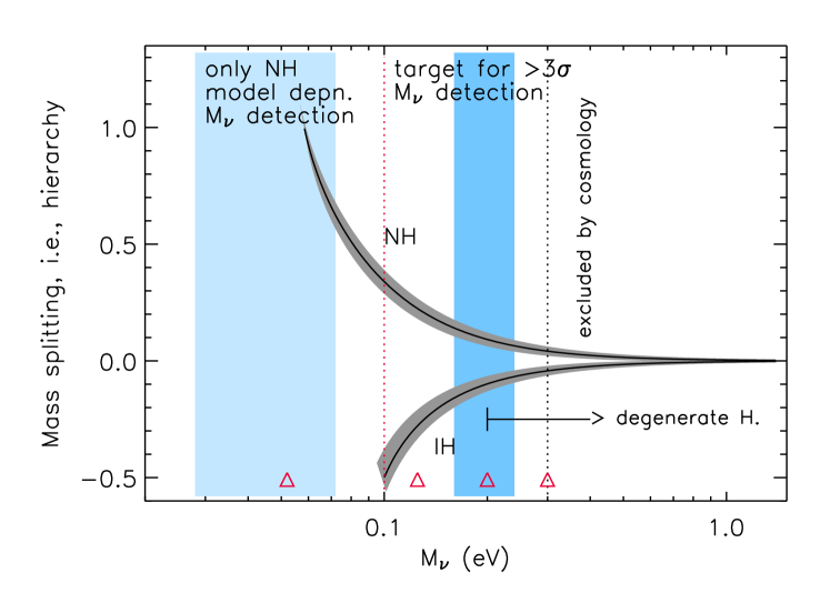
A detection of the cosmic relic neutrino background (RNG) with cosmological experiments would be a spectacular confirmation of our model for the early Universe and a window into one of the oldest relic components of our Universe besides the one represented by the stochastic gravitational wave background. This consideration prompts us to examine whether future galaxy redshift surveys probing LSS will be able to detect the signature of the neutrino background and to determine the neutrino absolute mass scale.

Beyond neutrino mass, cosmology is also sensitive to the number of neutrino species. In the standard model for particle physics there are three neutrinos; they decouple early in the cosmic history and then contribute to the relativistic energy density (i.e. as if they were radiation) with an effective number of neutrino species $N_{\rm eff}=3.046$ (e.g. [1]) until they become non-relativistic. Cosmology is sensitive to the physical energy density of relativistic particles, which include photons and neutrinos: $\Omega_{r}=\Omega_{\gamma}+N_{\rm eff}\Omega_{\nu}$, where $\Omega_{\gamma}$ and $\Omega_{\nu}$ are the energy density in photons and in one active neutrino species, respectively. CMB observations have constrained exquisitely well $\Omega_{\gamma}$, thus constraints in $\Omega_{\rm r}$ can be used to study neutrino properties. Deviations from $N_{\rm eff}=3.046$ would indicate non-standard neutrino properties or additional effective relativistic species. While the motivation for considering deviations from the standard model in the form of extra neutrino species has now disappeared [25, 26, 27], departures from the standard $N_{\rm eff}$ value could arise from decay of dark-matter particles [28, 29, 30, 31], early quintessence [32], or more exotic models [33].

Relativistic particles affect the CMB and the matter power spectrum in two ways: a) through their anisotropic stress [34, 5], and b) through their relativistic energy density which alters the epoch of matter radiation equality. The ratio of CMB peak heights constrains matter-radiation equality yielding a degeneracy between $N_{\rm eff}$ and $\Omega_{m}h^{2}$. This degeneracy can be lifted by adding either cosmic expansion history data [35, 36, 37] or adding the large-scale shape of the matter power spectrum: the power spectrum turnover scale is also related to matter-radiation equality given by the parameter $\Gamma\sim\Omega_{m}h$ (note the different scaling with $h$ compared to the CMB constraint). LSS surveys can yield a measurement, at the same time, of both the cosmic expansion history (via the Baryon Acoustic Oscillations (BAO) signal), and the large scale turnover of the power spectrum. Present constraints are already competitive with nucleosynthesis constraints, and future data will offer the possibility to test consistency of the standard paradigm for the early Universe. In fact, nucleosynthesis constraints rely on physics describing the Universe when its energy scale was $T\sim$ MeV, while cosmological constraints rely on physics at $T\sim eV$.

In this paper we forecast errors on the total neutrino mass $M_{\nu}$ and the effective number of relativistic species $N_{\rm eff}$ by combining Planck priors with data from future space-based galaxy redshift surveys in the near-IR. In particular, we consider two main survey strategies:

• The first approach is to use “multi-slit” spectroscopy aimed at observing a pure magnitude-limited sample of galaxies selected in the near-IR (e.g. in the H-band at 1.6 $\mu$m) with a limiting magnitude appropriate to cover the desired redshift range. Examples of this approach are given by instruments where the efficient multi-slit capability is provided by micro-shutter arrays (MSA) (e.g. JEDI [38, 39, 40]), or by digital micromirror devices (DMD) (e.g. SPACE [41] and possibly WFIRST in the future). With the multi-slit approach, all galaxy types (from passive ellipticals to starbursts) are observed, typically at $0<z<2-3$, if the observations are done in the near-IR, and provided that the targets are randomly selected from the magnitude-limited galaxy sample.

• The second approach is based on slitless spectroscopy (e.g. Euclid and JDEM [42, 43, 44]) which, due to stronger sky background, is sensitive mostly to galaxies with emission lines (i.e. star-forming and AGN systems), and uses mainly H$\alpha$ as a redshift tracer if the observations are done in the near-IR to cover the redshift range $0.5<z<2$.

Forthcoming surveys will also have a weak gravitational lensing component, which will also be used to constrain neutrino properties (see e.g. [9]). Here we concentrate on galaxy clustering as an independent and complementary probe.

The rest of the paper is organised as follows. In § 2 we review our method and the employed modelling. In § 3 we report the characteristics of the galaxy surveys considered in this work, and in § 4 we describe the adopted fiducial models and the explored space of cosmological parameters. In § 5 we present our results on the forecasted errors on the neutrino mass and number of neutrino species, and final in § 6 we draw our conclusions.

2 Fisher matrix approach: $P(k)$–method

In this paper we adopt the Fisher matrix formalism to make predictions on neutrino masses and relativistic degrees of freedom from future galaxy redshift surveys.

The Fisher matrix is defined as the second derivative of the natural logarithm of the likelihood surface about the maximum. In the approximation that the posterior distribution for the parameters is a multivariate Gaussian with mean $\mbox{\boldmath${\mu}$}\equiv\langle{\bf x}\rangle$ and covariance matrix ${\bf C}\equiv\langle{\bf x}{\bf x}^{t}\rangle-\mbox{\boldmath${\mu}$}\mbox{\boldmath${\mu}$}^{t}$, its elements are given by [45, 46, 47, 48]

$$F_{ij}=\frac{1}{2}{\rm Tr}\left[{\bf C}^{-1}{\partial{\bf C}\over\partial\theta_{i}}{\bf C}^{-1}{\partial{\bf C}\over\partial\theta_{j}}\right]+{\partial\mbox{\boldmath${\mu}$}\over\partial\theta_{i}}^{t}{\bf C}^{-1}{\partial\mbox{\boldmath${\mu}$}\over\partial\theta_{j}}.$$ (1)

where ${\bf x}$ is a N-dimensional vector representing the data set, whose components $x_{i}$ are the fluctuations in the galaxy density relative to the mean in $N$ disjoint cells that cover the three-dimensional survey volume in a fine grid. The $\{\theta_{i}\}$ denote the cosmological parameters within the assumed fiducial cosmology.

In order to explore the cosmological parameter constraints from a given redshift survey, we need to specify the measurement uncertainties of the galaxy power spectrum. In general, the statistical error on the measurement of the galaxy power spectrum $P_{\rm g}(k)$ at a given wave-number bin is [49]

$$\left[\frac{\Delta P_{\rm g}}{P_{\rm g}}\right]^{2}=\frac{2(2\pi)^{2}}{V_{\rm survey}k^{2}\Delta k\Delta\mu}\left[1+\frac{1}{n_{\rm g}P_{\rm g}}\right]^{2},$$ (2)

where $n_{\rm g}$ is the mean number density of galaxies, $V_{\rm survey}$ is the comoving survey volume of the galaxy survey, and $\mu$ is the cosine of the angle between $\bf{k}$ and the line-of-sight direction $\mu=\vec{k}\cdot\hat{r}/k$.

In general, the observed galaxy power spectrum is different from the true spectrum, and it can be reconstructed approximately assuming a reference cosmology (which we consider to be our fiducial cosmology) as (e.g. [50])

$$P_{\rm obs}(k_{{\rm ref}\perp},k_{{\rm ref}\parallel},z)=\frac{D\!_{A}(z)_{\rm ref}^{2}H(z)}{D\!_{A}(z)^{2}H(z)_{\rm ref}}P_{\rm g}(k_{{\rm ref}\perp},k_{{\rm ref}\parallel},z)+P_{\rm shot}\,,$$ (3)

where

$$P_{\rm g}(k_{{\rm ref}\perp},k_{{\rm ref}\parallel},z)=b(z)^{2}\left[1+\beta(z,k)\frac{k_{{\rm ref}\parallel}^{2}}{k_{{\rm ref}\perp}^{2}+k_{{\rm ref}\parallel}^{2}}\right]^{2}\times P_{{\rm matter}}(k,z)\,.$$ (4)

In Eq. (3), $H(z)$ and $D_{A}(z)$ are the Hubble parameter and the angular diameter distance, respectively, and the prefactor $(D\!_{A}(z)_{\rm ref}^{2}H(z))/(D\!_{A}(z)^{2}H(z)_{\rm ref})$ encapsulates the geometrical distortions due to the Alcock-Paczynski effect [50, 51]. Their values in the reference cosmology are distinguished by the subscript ‘ref’, while those in the true cosmology have no subscript. $k_{\perp}$ and $k_{\parallel}$ are the wave-numbers across and along the line of sight in the true cosmology, and they are related to the wave-numbers calculated assuming the reference cosmology by $k_{{\rm ref}\perp}=k_{\perp}D_{A}(z)/D_{A}(z)_{\rm ref}$ and $k_{{\rm ref}\parallel}=k_{\parallel}H(z)_{\rm ref}/H(z)$. $P_{shot}$ is the unknown white shot noise that remains even after the conventional shot noise of inverse number density has been subtracted [50], and which could arise from galaxy clustering bias even on large scales due to local bias [52]. In Eq. (4), $b(z)$ is the linear bias factor between galaxy and matter density distributions, and $\beta(z,k)=f_{g}(z,k)/b(z)$ is the linear redshift-space distortion parameter [53], which in the presence of massive neutrinos depends on both redshift and wave-numbers, since in this case the linear growth rate $f_{g}(z,k)$ is scale dependent even at the linear level. We estimate $f_{g}(z,k)$ using the fitting formula of Ref. [11] (see the bottom-right panel of Fig. 2). For the linear matter power spectrum $P_{{\rm matter}}(k,z)$, we can encapsulate the effect of massive neutrino free-streaming into a redshift dependent total matter linear transfer function $T(k,z)$ [54, 55, 56], so that $P_{{\rm matter}}(k,z)$ in Eq. (3) takes the form

$$P_{{\rm matter}}(k,z)=\frac{8\pi^{2}c^{4}k_{0}\Delta^{2}_{\cal R}(k_{0})}{25H_{0}^{4}\Omega_{m}^{2}}T^{2}(k,z)\left[\frac{G(z)}{G(z=0)}\right]^{2}\left(\frac{k}{k_{0}}\right)^{n_{s}}e^{-k^{2}\mu^{2}\sigma_{r}^{2}},$$ (5)

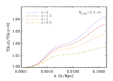
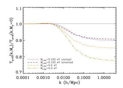
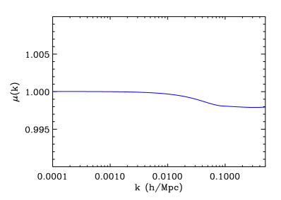
where $G(z)$ is the usual scale independent linear growth-factor in the absence of massive neutrino free-streaming, i.e. for $k\rightarrow 0$ (see Eq. (25) in Ref. [56]), whose fiducial value in each redshift bin is computed through numerical integration of the differential equations governing the growth of linear perturbations in the presence of dark-energy [57]. The redshift-dependent linear transfer function $T(k,z)$ depends on matter, baryon and massive neutrino densities (neglecting dark-energy at early times), and is computed in each redshift bin using CAMB [58]. As an example of its redshift dependence, in the top-left panel of Fig. 2 we consider the linear transfer function and show the ratio $T(k,z)/T(k,z=0)$ computed with CAMB at redshifts $z=0.5,1,1.5,2$ for a total neutrino mass $M_{\nu}=0.3$ eV. On the other hand, in the top-right panel of Fig. 2, as an example of the neutrino free-streaming effect, we fix the redshift at $z=0$ and compute, for different neutrino masses, the ratio of the linear transfer function to the linear transfer function in absence of massive neutrinos. The power suppression due to neutrino free-streaming is evident and increases with the neutrino mass as well as the free-streaming scale. This suppression is also slightly dependent on the assumed mass hierarchy, as the blue-dotted and red-dashed lines clearly show.

Figure 2: Top Left: Ratio $T(k,z)/T(k,z=0)$ of the linear transfer functions computed with CAMB at redshifts $z=0,0.5,1,1.5,2$, for a fiducial cosmology with a total neutrino mass $M_{\nu}=0.3$ eV and a degenerate mass spectrum. Top Right: Ratio $T_{z=0}(k,M_{\nu})/T_{z=0}(k,M_{\nu}=0)$ between the linear transfer functions computed with CAMB for the different $M_{\nu}$–cosmologies described in Sec. 4 and the linear transfer function obtained assuming massless neutrinos. Bottom Left: Ratio $T_{z=0}(k,N_{\rm eff}=4)/T_{z=0}(k,N_{\rm eff}=3.03)$ between the linear transfer functions computed with CAMB assuming massless neutrinos and an effective number of relativistic species $N_{\rm eff}=4$ and $N_{\rm eff}=3.04$, respectively. Bottom Right: the function $\mu(k,f_{\nu},\Omega_{de})\equiv f_{g}(M_{\nu}\neq 0)/f_{g}(M_{\nu}=0)$, where $f_{\nu}=\Omega_{\nu}/\Omega_{m}$. Note that $\mu(k,f_{\nu},\Omega_{de})$ represents the scale dependent correction to $f_{g}(z)$, evaluated at $M_{\nu}=0.05$.

In Eq. (5) we have added the damping factor $e^{-k^{2}\mu^{2}\sigma_{r}^{2}}$, due to redshift uncertainties, where $\sigma_{r}=(\partial r/\partial z)\sigma_{z}$, $r(z)$ being the comoving distance [59, 50], and we have assumed the power spectrum of primordial curvature perturbations, $P_{\cal R}(k)$, to be

$$\Delta^{2}_{\cal R}(k)\equiv\frac{k^{3}P_{\cal R}(k)}{2\pi^{2}}=\Delta^{2}_{\cal R}(k_{0})\left(\frac{k}{k_{0}}\right)^{n_{s}},$$ (6)

where $k_{0}=0.002$/Mpc, $\Delta^{2}_{\cal R}(k_{0})|_{\rm fid}=2.45\times 10^{-9}$ is the dimensionless amplitude of the primordial curvature perturbations evaluated at a pivot scale $k_{0}$, and $n_{s}$ is the scalar spectral index [60].

With the aim to make forecasts on the ability of future redshift galaxy surveys to constrain neutrino features, adopting different spectroscopic approaches (as discussed in §3), in this work we consider separately the effect on $P_{\rm obs}$ of the total neutrino mass $M_{\nu}$ and the number of relativistic degrees of freedom $N_{\rm eff}$, exploiting information from both the galaxy power spectrum shape and BAO distance indicators. In §5.6 we will analyse also the impact on neutrino mass constraints due to the inclusion of both growth–information and a Gaussian damping due to random peculiar velocities.

In each redshift shell, with size $\Delta z=0.1$ and centred at redshift $z_{i}$, we choose the following set of parameters to describe $P_{\rm obs}(k_{{\rm ref}\perp},k_{{\rm ref}\parallel},z)$:

$$\left\{H(z_{i}),D_{A}(z_{i}),\bar{G}(z_{i}),\beta(z_{i},k),P_{shot}^{i},\omega_{m},\omega_{b},\zeta,n_{s},h\right\},$$ (7)

where $\zeta=N_{\rm eff}$ or $\zeta=\omega_{\nu}\equiv\Omega_{\nu}h^{2}$ (depending on the assumed fiducial cosmology, see §4), $\omega_{m}=\Omega_{m}h^{2}$, $\omega_{b}=\Omega_{b}h^{2}$, where $h$ is given by $H_{0}=100h$ km s^-1 Mpc^-1 , $H_{0}$ being the Hubble constant. $\Omega_{m}$, $\Omega_{\nu}=M_{\nu}/(h^{2}93.8){\rm eV}$, and $\Omega_{b}$ are respectively the total matter, massive neutrino, and baryon present-day energy densities, in units of the critical energy density of the Universe. Finally, since $G(z)$, $b(z)$, and the power spectrum normalisation $P_{0}$ are completely degenerate, we have introduced the quantity $\bar{G}(z_{i})=(P_{0})^{0.5}b(z_{i})G(z_{i})/G(z_{0})$ [61].

In the limit where the survey volume is much larger than the scale of any features in $P_{\rm obs}(k)$, it has been shown [62] that it is possible to redefine $x_{n}$ to be not the density fluctuation in the $n^{th}$ spatial volume element, but the average power measured with the FKP method [49] in a thin shell of radius $k_{n}$ in Fourier space. Under these assumptions the redshift survey Fisher matrix can be approximated as [46, 62]

$$F_{ij}^{\rm LSS} = \int_{\vec{k}_{\rm min}}^{\vec{k}_{\rm max}}\frac{\partial\ln P_{\rm obs}(\vec{k})}{\partial p_{i}}\frac{\partial\ln P_{\rm obs}(\vec{k})}{\partial p_{j}}V_{\rm eff}(\vec{k})\frac{d\vec{k}}{2(2\pi)^{3}}$$

$$= \int_{-1}^{1}\int_{k_{\rm min}}^{k_{\rm max}}\frac{\partial\ln P_{\rm obs}(k,\mu)}{\partial p_{i}}\frac{\partial\ln P_{\rm obs}(k,\mu)}{\partial p_{j}}V_{\rm eff}(k,\mu)\frac{2\pi k^{2}dkd\mu}{2(2\pi)^{3}}$$

where the derivatives are evaluated at the parameter values $p_{i}$ of the fiducial model, and $V_{\rm eff}$ is the effective volume of the survey:

$$V_{\rm eff}(k,\mu)=\left[\frac{{n_{\rm g}}P_{\rm g}(k,\mu)}{{n_{\rm g}}P_{\rm g}(k,\mu)+1}\right]^{2}V_{\rm survey},$$ (9)

where we have assumed that the comoving number density $n_{\rm g}$ is constant in position. Due to azimuthal symmetry around the line of sight, the three-dimensional galaxy redshift power spectrum $P_{\rm obs}(\vec{k})$ depends only on $k$ and $\mu$, i.e. is reduced to two dimensions by symmetry [50].

To minimise nonlinear effects, we restrict wave-numbers to the quasi-linear regime, so that $k_{\rm max}$ is given by requiring that the variance of matter fluctuations in a sphere of radius $R$ is $\sigma^{2}(R)=0.25$ for $R=\pi/(2k_{\rm max})$. This gives $k_{\rm max}\simeq 0.1h{\rm\;Mpc^{-1}}$ at $z=0$ and $k_{\rm max}\simeq 0.2h{\rm\;Mpc^{-1}}$ at $z=1$, well within the quasi-linear regime. In addition, we impose a uniform upper limit of $k_{\rm max}\leq 0.2h{\rm\;Mpc^{-1}}$ (i.e. $k_{\rm max}=0.2h{\rm\;Mpc^{-1}}$ at $z>1$), to ensure that we are only considering the conservative linear regime, essentially unaffected by nonlinear effects. In each bin we adopt $k_{\rm min}=10^{-4}h$/Mpc, and we have verified that changing the survey maximum scale $k_{\rm min}$ with the shell volume has almost no effect on the results.

For the moment, we do not include information from the amplitude $\bar{G}(z_{i})$ and the redshift space distortions $\beta(z_{i},k)$, so we marginalise over these parameters and also over $P_{shot}^{i}$. Then we project $\mbox{\bf p}=\{H(z_{i}),D_{A}(z_{i}),\omega_{m},\omega_{b},\zeta,n_{s},h\}$ into the final sets q of cosmological parameters described in §4 [63, 64]. In this way we adopt the so-called “full $P(k)$–method, marginalised over growth–information” [65], and, to change from one set of parameters to another, we use [63]

$$F_{\alpha\beta}^{\rm LSS}=\sum_{ij}\frac{\partial p_{i}}{\partial q_{\alpha}}\,F_{ij}^{\rm LSS}\,\frac{\partial p_{j}}{\partial q_{\beta}},$$ (10)

where $F_{\alpha\beta}^{\rm LSS}$ is the survey Fisher matrix for the set of parameters q, and $F_{ij}^{\rm LSS}$ is the survey Fisher matrix for the set of equivalent parameters p.

We derive neutrino constraints with and without cosmic microwave background (CMB) priors; to this end we use the specifications of the Planck satellite. As explained in Appendix A, in order to describe CMB temperature and polarisation power spectra, we choose the parameter set $\vec{\theta}=\{\omega_{m},\omega_{b},\zeta,100\theta_{S},\ln(10^{10}\Delta^{2}_{\cal R}(k_{0})),n_{S},\tau\}$, where $\theta_{S}$ is the angular size of the sound horizon at last scattering, and $\tau$ is the optical depth due to reionisation. After marginalisation over the optical depth, we propagate the Planck CMB Fisher matrix $F_{ij}^{\rm CMB}$ into the final sets of parameters q, by using the appropriate Jacobian for the involved parameter transformation.

The 1–$\sigma$ error on $q_{\alpha}$ marginalised over the other parameters is $\sigma(q_{\alpha})=\sqrt{({F}^{-1})_{\alpha\alpha}}$, where ${F}^{-1}$ is the inverse of the Fisher matrix. We then consider constraints in a two-parameter subspace, marginalising over the remaining parameters, in order to study the covariance between $N_{\rm eff}$ or $M_{\nu}$ and the other cosmological parameters, respectively.

Furthermore, to quantify the level of degeneracy between the different parameters, we estimate the so-called correlation coefficients, given by

$$r\equiv\frac{({F}^{-1})_{p_{\alpha}p_{\beta}}}{\sqrt{({F}^{-1})_{p_{\alpha}p_{\alpha}}({F}^{-1})_{p_{\beta}p_{\beta}}}},$$ (11)

where $p_{\alpha}$ denotes one of the model parameters. When the coefficient $|r|=1$, the two parameters are totally degenerate, while $r=0$ means they are uncorrelated.

We evaluate $\sigma(q_{\alpha})$ and $r$ both from survey data $F^{\rm LSS}_{\alpha\beta}$, and from the combined CMB+LSS data $F_{\alpha\beta}=F^{\rm LSS}_{\alpha\beta}+F^{\rm CMB}_{\alpha\beta}$.

3 Surveys: two spectroscopic strategies

In this work we forecast neutrino constraints using two different spectroscopic approaches. In particular, as mentioned in §1, we consider the cases relative to two space mission concepts under study:

• a EUCLID-like survey of H$\alpha$ emission line galaxies, based on slitless spectroscopy of the sky. We adopt the empirical redshift distribution of H$\alpha$ emission line galaxies derived by [66] from observed H$\alpha$ luminosity functions, and the bias function derived by [67] using a galaxy formation simulation. In particular, we choose a flux limit of 4$\times 10^{-16}$erg s^-1cm^-1, a survey area of 20,000 deg², a redshift success rate $e=0.5$, a redshift accuracy of $\sigma_{z}/(1+z)\leq 0.001$, and a redshift range $0.5\leq z\leq 2.1$. The total number of galaxies with redshift errors $\sigma_{z}/(1+z)\leq 0.001$ from a slitless survey is well approximated by [65]

  $$\frac{N_{gal}}{10^{6}}=276.74\,\frac{[area]}{20000}\,\frac{e}{0.5}\,\left(\bar{f}\right)^{-0.9\left(\bar{f}\right)^{0.14}},$$ (12)

  where $\bar{f}\equiv f/[10^{-16}$erg s^-1cm^-2]. For this type of space-based slitless redshift survey we add in our forecasts also information from the ongoing Sloan Digital Sky Survey III (SDSS-III) Baryon Oscillation Spectroscopic Survey (BOSS) of luminous red galaxies (LRG). For this galaxy survey we assume that the LRG redshifts are measured over $0.1<z<0.5$ with standard deviation $\sigma_{z}/(1+z)=0.001$, for a galaxy population with a fixed number density of $n=3\times 10^{-4}h^{3}$Mpc^-3, and a fixed linear bias of $b=1.7$ [68], over a survey area of 10,000 deg².

• a H-band magnitude limited survey of randomly sampled galaxies enabled by multi-slit spectroscopy (e.g., SPACE [41], JEDI [38, 39, 40], and possibly WFIRST in the future). To predict galaxy densities for such surveys we use the empirical galaxy redshift distribution compiled by Zamorani et al. from existing data [43], and we use predictions of galaxy bias from galaxy formation simulations [67]. We consider multi-slit surveys with a limiting magnitude of $H_{AB}$=22, a redshift success rate of 90%, a sampling rate of 35%, a survey area of 20,000 deg², a redshift accuracy of $\sigma_{z}/(1+z)\leq 0.001$, and a redshift range $0.1\leq z\leq 2.1$. The total number of galaxies with redshift errors $\sigma_{z}/(1+z)\leq 0.001$ from a multi-slit survey is well approximated by [65]

  $$\frac{N_{gal}}{10^{6}}=\left[192.21+197.03\,(H_{AB}-22)^{1.3}\right]\,\frac{[area]}{20000}\,\frac{e}{0.9\times 0.35}.$$ (13)

Note that BOSS data are not added to the multi-slit galaxy redshift survey, since the latter has redshift ranges that extend to $z\sim 0.1$ [41, 43]. The case is different for H$\alpha$ flux selected galaxies observed from space, since a wavelength range between 1 and 2 $\mu$m naturally imposes a redshift range $0.52<z<2.05$ in which H$\alpha$ will be visible [43].

Furthermore, the bias functions for H$\alpha$ flux and H-band magnitude selected galaxies increase with redshift, with the former being less strongly biased than the latter [67]. In fact, the H-band traces massive structures (similar to selecting galaxies in the K-band), which makes them strongly biased. Star forming galaxies (which are selected by H$\alpha$ flux), on the other hand, appear to avoid the cores of clusters and populate the filaments of the dark-matter structure, making them less biased than H-band galaxies [67].

In conclusion, multi-slit surveys allow accurate redshift measurement for a larger number of galaxies (and these galaxies are more biased tracers of large-scale structure than star-forming galaxies), and over a greater redshift range (extending to $z\sim 0.1$) than slitless surveys. This can improve the constraints on neutrino masses, and, moreover, the ability to split a galaxy catalogue into red and blue galaxies could provide an important diagnostic test of potential systematic errors when measuring neutrino masses [69]. However, multi-slit surveys have substantially stronger requirements in instrumentation and mission implementation [41].

4 Fiducial cosmologies: $M_{\nu}$ and $N_{\rm eff}$

The Fisher matrix approach propagates errors of galaxy power spectrum measurements Eq. (2) into errors of the cosmological parameters which characterise the underlying fiducial cosmology. According to the latest observations (e.g. [5] and refs. therein), we assume the fiducial cosmological model adopted in the Euclid Assessment Study Report [43] with the exception that we normalise to the amplitude of the primordial curvature perturbations $\Delta^{2}_{\cal R}(k_{0})$ instead of $\sigma_{8}$: $\Omega_{m}=0.25$, $h=0.7$, $\Delta^{2}_{\cal R}(k_{0})=2.45\times 10^{-9}$, $\Omega_{b}=0.0445$, $n_{s}=1$. We consider neither primordial gravitational waves nor a scale dependent component of the scalar spectral index, and assume the matter energy density $\Omega_{m}$ to include the neutrino contribution when neutrinos are non-relativistic

$$\Omega_{m}=\Omega_{c}+\Omega_{b}+\Omega_{\nu}~{},$$ (14)

Moreover, we also assume dark-energy to be a cosmic fluid described by a redshift dependent equation of state

$$w_{de}(z)=\frac{p_{de}(z)}{\rho_{de}(z)}$$ (15)

where $p_{de}$ and $\rho_{de}$ represent respectively the pressure and energy density of the dark-energy fluid.

This in turn yields a redshift dependent dark-energy density

$$\rho_{de}(z)=\rho_{de}(0)\exp\left[3\int_{0}^{z}\frac{1+w(z^{\prime})}{1+z^{\prime}}dz^{\prime}\right],$$ (16)

for which we take a fiducial value $\Omega_{de}=0.75$. Finally, to compute our forecasts on dark-energy parameters, we adopt the widely used linear dark-energy equation of state [70, 71]

$$w_{de}(a)=w_{0}+(1-a)w_{a},$$ (17)

where $a\equiv 1/(1+z)$ is the scale factor normalised to unity at present, and we assume as fiducial values $w_{0}=-0.95$ and $w_{a}=0$, which lie well within the current $95$% C.L. limits. In what follows, the dark-energy figure of merit (FoM) will be computed in terms of the conventional FoM for ($w_{0}$,$w_{a}$) as proposed by DETF [72] to compare dark-energy surveys.

We will constraint the following final set of eight parameters

$$\mbox{\bf q}=\left\{\Omega_{m},\Omega_{de},h,\Delta^{2}_{\cal R}(k_{0}),\Omega_{b},w_{0},w_{a},n_{s}\right\},$$ (18)

which constitutes what we call our “base” parameters, to which we add the $\zeta$ parameter as we explain below.

In what follows, we will consider six different fiducial models matching our “base” fiducial $\Lambda$CDM cosmology, in which we adopt the same fiducial values for the eight “base” parameters. Then we specify the assumed cosmological models:

• The first model assumes a $N_{\rm eff}$–cosmology, where neutrinos are effectively massless but the the number of relativistic species $\zeta\equiv N_{\rm eff}$ can deviate from the standard value $N_{\rm eff}=3.04$. In this case the fiducial value $N_{\rm eff}|_{\rm fid}=3.04$ is chosen, fixing $M_{\nu}={\rm const}=0$ [25]. $N_{\rm eff}$ is given by the energy density associated to the total radiation

  $$\Omega_{r}=\Omega_{\gamma}\left(1+0.2271N_{\rm eff}\right)~{},$$ (19)

  where $\Omega_{\gamma}=2.469\times 10^{-5}h^{-2}$ is the present-day photon energy density parameter for $T_{\rm cmb}=2.725$ K [73].

• The remaining models assume a $M_{\nu}$–cosmology, where $N_{\rm eff}$ is fixed at the fiducial value and $\zeta\equiv M_{\nu}$ is allowed to vary accordingly to the assumed fiducial neutrino mass spectrum [23]. In this case, we choose the following five fiducial values for the total neutrino mass consistent with current data [74, 5]:

  $$M_{\nu}|_{\rm fid}=\Bigg{\{}\begin{array}[]{cc}0.3,0.2\;{\rm eV}&\mbox{for degenerate spectrum}\\ 0.125\;{\rm eV}&\mbox{for inverted hierarchy}\\ 0.125,0.05\;{\rm eV}&\mbox{for normal hierarchy}\end{array}$$ (23)

The motivation for considering different fiducial models is that the dependence of the power spectrum on $M_{\nu}$ is nonlinear and thus the size of the forecasted error bar on $M_{\nu}$ depends on the fiducial value chosen.

At the CMB level, if neutrinos are still relativistic at the decoupling epoch, $z\simeq 1090$, i.e. if the mass of the heaviest neutrino specie is $m_{\nu}<0.58$ eV, massive neutrinos do not affect the CMB power spectra, except through the gravitational lensing effect [73, 6, 7], and, as a consequence, the dark-energy equation of state $w_{de}$ is not degenerate with the neutrino mass. However, the limit on the the sum of neutrino masses degrades significantly when the dark-energy equation of state is a function of redshift as we assume in the present work, since dark-energy and massive neutrinos both affect the growth rate of structures [75]. However, as we will show in the next section, the combination of CMB and LSS probes reduces or even breaks these degeneracies. The same does not happen for the number of relativistic species $N_{\rm eff}$. Moreover, the degeneracies between $M_{\nu}$ and the other cosmological parameters can increase as the number of free parameters of the model increases, which could potentially bias the results for large $k$ values [69]. As evident from Eqs. (3)-(4), the model adopted in this paper falls within the two bias parameter models discussed in Ref. [69], which seem to mimic accurately the broad features of galaxy bias and redshift-space distortions from SDSS, leading to consistent constraints in the presence of massive neutrinos.

Table 1: Parameter 1-$\sigma$ errors for slitless spectroscopy

			slitless+BOSS
fiducial$\to$	$M_{\nu}$=0.3 eVa	$M_{\nu}$=0.2 eVa	$M_{\nu}$=0.125 eVb	$M_{\nu}$=0.125 eVc	$M_{\nu}$=0.05 eVb	$N_{\rm eff}$=3.04d
$\Omega_{m}$	$0.0140$	$0.0137$	$0.0139$	$0.0138$	$0.0137$	$0.0124$
$\Omega_{de}$	$0.0260$	$0.0265$	$0.0258$	$0.0257$	$0.0253$	$0.0256$
$\Omega_{b}$	$0.0032$	$0.0031$	$0.0032$	$0.0032$	$0.0032$	$0.0034$
$h$	$0.0116$	$0.0112$	$0.0113$	$0.0114$	$0.0113$	$0.0137$
$M_{\nu}$	$0.1459$	$0.1461$	$0.1795$	$0.1435$	$0.1428$	$--$
$N_{\rm eff}$	$--$	$--$	$--$	$--$	$--$	$0.5435$
$ns$	$0.0233$	$0.0225$	$0.0314$	$0.0228$	$0.0220$	$0.0326$
$w_{0}$	$0.0815$	$0.0837$	$0.0812$	$0.0808$	$0.0801$	$0.0807$
$w_{a}$	$0.3461$	$0.3573$	$0.3450$	$0.3440$	$0.3386$	$0.3324$
FoM	$51.75$	$48.44$	$52.44$	$52.68$	$54.25$	$55.23$
			slitless+BOSS+Planck
$\Omega_{m}$	$0.0034$	$0.0035$	$0.0033$	$0.0035$	$0.0035$	$0.0031$
$\Omega_{de}$	$0.0064$	$0.0064$	$0.0062$	$0.0064$	$0.0065$	$0.0064$
$\Omega_{b}$	$0.0006$	$0.0056$	$0.0006$	$0.0005$	$0.0005$	$0.0005$
$h$	$0.0043$	$0.0043$	$0.0043$	$0.0043$	$0.0042$	$0.0046$
$M_{\nu}$	$0.0347$	$0.0433$	$0.0311$	$0.0441$	$0.0526$	$--$
$N_{\rm eff}$	$--$	$--$	$--$	$--$	$--$	$0.0865$
$ns$	$0.0022$	$0.0022$	$0.0022$	$0.0022$	$0.0022$	$0.0041$
$w_{0}$	$0.0732$	$0.0721$	$0.0716$	$0.0715$	$0.0709$	$0.0705$
$w_{a}$	$0.1760$	$0.1742$	$0.1713$	$0.1725$	$0.1722$	$0.1664$
$\Delta^{2}_{\cal R}(k_{0})$	$0.0250$	$0.0226$	$0.0226$	$0.0227$	$0.0244$	$0.0227$
FoM	$245.07$	$242.80$	$259.32$	$247.96$	$240.31$	$294.15$

^afor degenerate spectrum: $m_{1}\approx m_{2}\approx m_{3}$; ^bfor normal hierarchy: $m_{3}\neq 0$, $m_{1}\approx m_{2}\approx 0$
^cfor inverted hierarchy: $m_{1}\approx m_{2}$, $m_{3}\approx 0$; ^dfiducial cosmology with massless neutrinos

Table 2: Parameter 1-$\sigma$ errors for multi-slit spectroscopy

			multi-slit
fiducial$\to$	$M_{\nu}$=0.3 eVa	$M_{\nu}$=0.2 eVa	$M_{\nu}$=0.125 eVb	$M_{\nu}$=0.125 eVc	$M_{\nu}$=0.05 eVb	$N_{\rm eff}$=3.04d
$\Omega_{m}$	$0.0090$	$0.0091$	$0.0092$	$0.0090$	$0.0091$	$0.0086$
$\Omega_{de}$	$0.0179$	$0.0178$	$0.0177$	$0.0177$	$0.0176$	$0.0185$
$\Omega_{b}$	$0.0020$	$0.0020$	$0.0020$	$0.0020$	$0.0020$	$0.0023$
$h$	$0.0079$	$0.0078$	$0.0079$	$0.0079$	$0.0079$	$0.0098$
$M_{\nu}$	$0.1229$	$0.1113$	$0.1321$	$0.1110$	$0.1126$	$--$
$N_{\rm eff}$	$--$	$--$	$--$	$--$	$--$	$0.4059$
$ns$	$0.0190$	$0.0160$	$0.0221$	$0.0158$	$0.0151$	$0.0242$
$w_{0}$	$0.0617$	$0.0614$	$0.0619$	$0.0613$	$0.0612$	$0.0629$
$w_{a}$	$0.2399$	$0.2399$	$0.2411$	$0.2400$	$0.2389$	$0.2427$
FoM	$94.16$	$94.78$	$94.49$	$95.12$	$96.02$	$94.09$
			multi-slit+Planck
$\Omega_{m}$	$0.0026$	$0.0027$	$0.0026$	$0.0027$	$0.0028$	$0.0025$
$\Omega_{de}$	$0.0050$	$0.0051$	$0.0050$	$0.0051$	$0.0053$	$0.0054$
$\Omega_{b}$	$0.0004$	$0.0004$	$0.0004$	$0.0004$	$0.0004$	$0.0004$
$h$	$0.0033$	$0.0033$	$0.0033$	$0.0033$	$0.0033$	$0.0038$
$M_{\nu}$	$0.0296$	$0.0376$	$0.0268$	$0.0388$	$0.0463$	$--$
$N_{\rm eff}$	$--$	$--$	$--$	$--$	$--$	$0.0817$
$ns$	$0.0021$	$0.0021$	$0.0021$	$0.0021$	$0.0021$	$0.0039$
$w_{0}$	$0.0554$	$0.0552$	$0.0552$	$0.0552$	$0.0551$	$0.0551$
$w_{a}$	$0.1307$	$0.1311$	$0.1294$	$0.1309$	$0.1320$	$0.1274$
$\Delta^{2}_{\cal R}(k_{0})$	$0.0247$	$0.0242$	$0.0224$	$0.0224$	$0.0237$	$0.0226$
FoM	$391.39$	$376.55$	$399.17$	$377.41$	$359.33$	$441.78$

^afor degenerate spectrum: $m_{1}\approx m_{2}\approx m_{3}$; ^bfor normal hierarchy: $m_{3}\neq 0$, $m_{1}\approx m_{2}\approx 0$
^cfor inverted hierarchy: $m_{1}\approx m_{2}$, $m_{3}\approx 0$; ^dfiducial cosmology with massless neutrinos

Table 3: Neutrino correlation coefficients for slitless spectroscopy

			slitless+BOSS
fiducial$\to$	$M_{\nu}$=0.3 eVa	$M_{\nu}$=0.2 eVa	$M_{\nu}$=0.125 eVb	$M_{\nu}$=0.125 eVc	$M_{\nu}$=0.05 eVb	$N_{\rm eff}$=3.04d
$\Omega_{m}$	$0.601$	$0.573$	$0.554$	$0.549$	$0.544$	$-0.316$
$\Omega_{de}$	$-0.208$	$-0.188$	$-0.188$	$-0.182$	$-0.134$	$0.221$
$\Omega_{b}$	$0.323$	$0.331$	$0.232$	$0.303$	$0.249$	$-0.439$
$h$	$0.252$	$0.259$	$0.165$	$0.230$	$0.129$	$0.602$
$M_{\nu}$	$1$	$1$	$1$	$1$	$1$	$--$
$N_{\rm eff}$	$--$	$--$	$--$	$--$	$--$	$1$
$ns$	$0.567$	$0.340$	$0.717$	$0.338$	$0.364$	$0.763$
$w_{0}$	$0.325$	$0.310$	$0.311$	$0.298$	$0.310$	$-0.305$
$w_{a}$	$-0.463$	$-0.437$	$-0.424$	$-0.417$	$-0.413$	$0.307$
			slitless+BOSS+Planck
$\Omega_{m}$	$0.344$	$0.404$	$0.331$	$0.416$	$0.485$	$0.140$
$\Omega_{de}$	$-0.312$	$-0.371$	$-0.290$	$-0.361$	$-0.445$	$0.389$
$\Omega_{b}$	$-0.141$	$-0.131$	$-0.136$	$-0.117$	$-0.169$	$-0.062$
$h$	$0.019$	$0.007$	$0.023$	$0.006$	$0.019$	$0.414$
$M_{\nu}$	$1$	$1$	$1$	$1$	$1$	$--$
$N_{\rm eff}$	$--$	$--$	$--$	$--$	$--$	$1$
$ns$	$-0.089$	$-0.071$	$-0.034$	$0.048$	$0.020$	$0.844$
$w_{0}$	$0.011$	$0.025$	$0.008$	$0.029$	$0.031$	$0.001$
$w_{a}$	$-0.166$	$-0.202$	$-0.157$	$-0.204$	$-0.266$	$0.074$
$\Delta^{2}_{\cal R}(k_{0})$	$0.106$	$0.229$	$0.073$	$0.105$	$0.288$	$0.123$

^afor degenerate spectrum: $m_{1}\approx m_{2}\approx m_{3}$; ^bfor normal hierarchy: $m_{3}\neq 0$, $m_{1}\approx m_{2}\approx 0$
^cfor inverted hierarchy: $m_{1}\approx m_{2}$, $m_{3}\approx 0$; ^dfiducial cosmology with massless neutrinos

Table 4: Neutrino correlation coefficients for multi-slit spectroscopy

			multi-slit
fiducial$\to$	$M_{\nu}$=0.3 eVa	$M_{\nu}$=0.2 eVa	$M_{\nu}$=0.125 eVb	$M_{\nu}$=0.125 eVc	$M_{\nu}$=0.05 eVb	$N_{\rm eff}$=3.04d
$\Omega_{m}$	$0.607$	$0.578$	$0.577$	$0.561$	$0.544$	$-0.447$
$\Omega_{de}$	$-0.151$	$-0.144$	$-0.136$	$-0.136$	$-0.134$	$0.324$
$\Omega_{b}$	$0.284$	$0.292$	$0.217$	$0.271$	$0.249$	$-0.551$
$h$	$0.175$	$0.179$	$0.110$	$0.158$	$0.129$	$0.604$
$M_{\nu}$	$1$	$1$	$1$	$1$	$1$	$--$
$N_{\rm eff}$	$--$	$--$	$--$	$--$	$--$	$1$
$ns$	$0.640$	$0.442$	$0.758$	$0.434$	$0.364$	$0.814$
$w_{0}$	$0.341$	$0.326$	$0.342$	$0.315$	$0.310$	$-0.368$
$w_{a}$	$-0.468$	$-0.444$	$-0.444$	$-0.425$	$-0.413$	$0.407$
			multi-slit+Planck
$\Omega_{m}$	$0.355$	$0.422$	$0.337$	$0.437$	$0.485$	$0.130$
$\Omega_{de}$	$-0.319$	$-0.384$	$-0.292$	$-0.375$	$-0.445$	$0.472$
$\Omega_{b}$	$-0.201$	$-0.184$	$-0.195$	$-0.167$	$-0.169$	$-0.049$
$h$	$0.052$	$0.034$	$0.058$	$0.033$	$0.019$	$0.480$
$M_{\nu}$	$1$	$1$	$1$	$1$	$1$	$--$
$N_{\rm eff}$	$--$	$--$	$--$	$--$	$--$	$1$
$ns$	$0.015$	$0.013$	$0.046$	$0.029$	$0.020$	$0.842$
$w_{0}$	$-0.011$	$0.011$	$-0.015$	$0.016$	$0.031$	$0.005$
$w_{a}$	$-0.168$	$-0.217$	$-0.156$	$-0.222$	$-0.266$	$0.080$
$\Delta^{2}_{\cal R}(k_{0})$	$0.060$	$0.177$	$0.029$	$0.068$	$0.288$	$0.153$

^afor degenerate spectrum: $m_{1}\approx m_{2}\approx m_{3}$; ^bfor normal hierarchy: $m_{3}\neq 0$, $m_{1}\approx m_{2}\approx 0$
^cfor inverted hierarchy: $m_{1}\approx m_{2}$, $m_{3}\approx 0$; ^dfiducial cosmology with massless neutrinos

5 Results

In this Section we present the predicted 1–$\sigma$ marginalised errors and correlations for the cosmological parameters considered in this work, focusing on the total neutrino mass $M_{\nu}$ and the number of relativistic species $N_{\rm eff}$, and comparing the results between the two spectroscopic strategies described in §3. We show forecasts from LSS alone and in combination with Planck priors.

In Tables 1-2 we show the marginalised errors for the six fiducial cosmologies considered here, computed adopting slitless and multi-slit spectroscopy, respectively; in Tables 3-4 we report the corresponding correlation coefficients. Both LSS alone and LSS+CMB results are reported.

Figure 3: 2-parameter $M_{\nu}$-$q_{\alpha}$ joint contours with $q_{\alpha}=\Omega_{de},w_{0},w_{a},\Omega_{m}$ for the fiducial model with $M_{\nu}=0.3$ eV and a degenerate neutrino mass spectrum, obtained after combining the slitless survey data with BOSS data and Planck priors. The blue dotted line, the red dashed line and the orange dot-dashed line represent the 68$\%$ C.L., 95.4$\%$ C.L. and 99.73$\%$ C.L., respectively. The black solid line shows the 1-parameter confidence level at 1–$\sigma$.

Figure 4: 2-parameter $N_{\rm eff}$-$q_{\alpha}$ joint contours with $q_{\alpha}=\Omega_{de},w_{0},w_{a},n_{s}$ for the fiducial model with extra relativistic degrees of freedom $N_{\rm eff}=3.04$, obtained after combining the slitless survey data with BOSS data and Planck priors. The blue dotted line, the red dashed line and the orange dot-dashed line represent the 68$\%$ C.L., 95.4$\%$ C.L. and 99.73$\%$ C.L., respectively. The black solid line shows the 1-parameter confidence level at 1–$\sigma$.

Figure 5: 1-parameter confidence levels at 1-$\sigma$ for $M_{\nu}$ and $q_{\alpha}$ with $q_{\alpha}=\Omega_{de},w_{0},w_{a},\Omega_{m}$ for the fiducial model with $M_{\nu}=0.05$ eV and a neutrino mass spectrum with normal hierarchy, obtained after combining the survey data with Planck priors. The blue solid line and the red dashed one represent the slitles+BOSS– and multi-slit–surveys cases respectively, as described in Sec. 3.

Figure 6: 1-parameter confidence levels for $N_{\rm eff}$ and $q_{\alpha}$ with $q_{\alpha}=\Omega_{de},w_{0},w_{a},n_{s}$ for the fiducial model with $N_{\rm eff}=3.04$, obtained after combining the survey data with Planck priors. The blue solid line and the red dashed one represent the slitles+BOSS– and multi-slit–surveys cases respectively, as described in Sec. 3.

Figure 7: Top: $M_{\nu}$–errors, for $M_{\nu}|_{\rm fid}=0.05$ eV, as functions of the minimum redshift $z_{min}$ of the surveys, where we have fixed the maximum redshift $z_{max}=2.1$ for both the spectroscopic strategies. The lowest minimum redshifts considered are $z_{min}=0.5$ and $z_{min}=0.1$ for the slitless and multi-slit spectroscopies, respectively. Bottom: $M_{\nu}$–errors, for $M_{\nu}|_{\rm fid}=0.05$ eV, as functions of the maximum redshift $z_{max}$ of the surveys, where we have fixed the minimum redshifts $z_{min}=0.5$ and $z_{min}=0.1$ for the slitless and multi-slit spectroscopies, respectively.

Figure 8: Top: $N_{\rm eff}$–errors as functions of the minimum redshift $z_{min}$ of the surveys, where we have fixed the maximum redshift $z_{max}=2.1$ for both the spectroscopic strategies. The lowest minimum redshifts considered are $z_{min}=0.5$ and $z_{min}=0.1$ for the slitless and multi-slit spectroscopies, respectively. Bottom: $N_{\rm eff}$–errors as functions of the maximum redshift $z_{max}$ of the surveys, where we have fixed the minimum redshifts $z_{min}=0.5$ and $z_{min}=0.1$ for the slitless and multi-slit spectroscopies, respectively.

Let us discuss the findings for the $M_{\nu}$– and $N_{\rm eff}$–cosmologies separately.

5.1 $M_{\nu}$–cosmology: Correlations

When considering forecasts from LSS alone, we find that $M_{\nu}$ is correlated with all the cosmological parameters affecting the galaxy power spectrum shape and BAO positions at scales $k\leq k_{\rm max}$ (see columns 2-6 in the upper panels of Tables 3-4). In particular, there is a quite strong positive correlation $r\sim 0.55$ between the total neutrino mass $M_{\nu}$ and the matter density $\Omega_{m}$. In fact, since neutrino free-streaming suppresses the total matter transfer function on scales smaller than the free-streaming scale $k_{\rm fs}$, increasing the neutrino mass produces on $T(k,z)$ the opposite effect than increasing the total matter content of the Universe. For the same reason, massive neutrinos mimic the effect of a red tilt on the galaxy power spectrum, resulting in a positive correlation between $M_{\nu}$ and the scalar spectral index $n_{s}$. Moreover, $M_{\nu}$ is also positively correlated to the baryon density $\Omega_{b}$ if the total matter content of the Universe is held fixed (a larger $\Omega_{b}$ enhances the BAO and the information content of $T(k,z)$). The correlation of $M_{\nu}$ with the remaining parameters $h$, $\Omega_{de}$, $w_{0}$, and $w_{a}$ can be explained looking at the Alcock-Paczynski prefactor in Eq. (3), and recalling that for the moment we are not including information from the amplitude of the galaxy power spectrum, since we marginalise over the bias, the growth factor, the redshift space distortions, and the power spectrum normalisation. In this case we have to consider the expression of $H(z)$ in presence of a non-vanishing spatial curvature of the Universe $\Omega_{\rm K}=1-\Omega_{m}-\Omega_{de}-\Omega_{r}$

$$H(z) = H_{0}\big{\{}\Omega_{r}[(1+z)^{4}-(1+z)^{2}]+\Omega_{m}[(1+z)^{3}-(1+z)^{2}]+$$ (24)

$$\Omega_{de}[(1+z)^{3(1+w_{0}+w_{a})}e^{3w_{a}(a-1)}-(1+z)^{2}]+(1+z)^{2}\big{\}}^{1/2},$$

and remember that $D\!_{A}(z)$ is related to the inverse of $H(z)$ Given the fiducial values of $h$, $\Omega_{de}$, $w_{0}$, and $w_{a}$, and varying each parameter at a time, we see from Eq. (24) that increasing $h$ or $w_{0}$ enhances the observed power spectrum $P_{\rm obs}$ in contrast to the suppression induced by the increase of the total neutrino mass, so that these parameters are positively correlated with $M_{\nu}$. On the contrary, from Eq. (24) and looking at the sign of the term $[(1+z)^{3(1+w_{0}+w_{a})}e^{3w_{a}(a-1)}-(1+z)^{2}]$, we also deduce that increasing $\Omega_{de}$ or $w_{a}$ produces on $P_{\rm obs}$ the same effect as a larger neutrino mass, so these parameters are negatively correlated or “anti-correlated” to $M_{\nu}$.

Except for the $n_{s}$ case, we find that the level of correlation is on the average stable against the value of the fiducial total neutrino mass and the spectroscopic strategy adopted. For what concerns the mass hierarchy, at a given $M_{\nu}|_{\rm fid}$, the $n_{s}$-$M_{\nu}$ correlation looks to be larger by $\sim 54\%-72\%$ for normal hierarchy in comparison to the inverted one, at least when information from LSS alone are used, and the effect is more evident for slitless spectroscopy. In contrast, the $h$-$M_{\nu}$ and $\Omega_{b}$-$M_{\nu}$ correlations slightly decrease by $\sim 34\%-24\%$ respectively, for normal hierarchy compared to the inverted hierarchy. This can be understood if we consider that, for the same $M_{\nu}|_{\rm fid}$, in the case of normal hierarchy, the transfer function is slightly less suppressed on the scales of interest with respect to the inverted one (see Fig. 2, and § 5.2 for further comments on the relation between forecasted $M_{\nu}$–errors and the neutrino mass hierarchy).

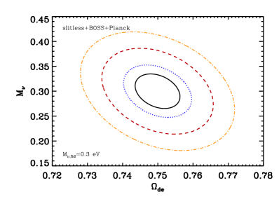
When Planck priors are added to the survey constraints, all degeneracies are either resolved or reduced, except for the covariance $M_{\nu}$-$\Omega_{de}$. In particular, the correlation between $M_{\nu}$ and $n_{s}$ is completely resolved, being reduced by $\sim$ one order of magnitude. In some cases, the correlation coefficient $r$ can even change sign (see columns 2-6 in the lower panels of Tables 3-4). This change in the behaviour of $r$ arises either due to the presence of dominant parameter degeneracies affecting the CMB spectrum, or because of marginalisation of a high-dimension parameter space down to two variables. To summarise, after the inclusion of Planck priors, the remaining dominant correlations among $M_{\nu}$ and the other cosmological parameters are $M_{\nu}$-$\Omega_{de}$, $M_{\nu}$-$\Omega_{m}$, and $M_{\nu}$-$w_{a}$.

5.2 $M_{\nu}$–cosmology: Forecasted error-bars

The 1–$\sigma$ errors of the parameters are shown in columns 2-6 of Tables 1-2. We see that, with respect to the slitless spectroscopy, the multi-slit spectroscopy is able to reduce the neutrino mass errors of about 20%-30%, depending on the fiducial neutrino mass, if LSS data alone are used. In addition, for the same $M_{\nu}|_{\rm fid}$, the 1–$\sigma$ error on total neutrino mass for normal hierarchy is $\sim 17\%-20\%$ larger than for the inverted one. It looks like that the matter power spectrum is less able to give information on the total neutrino mass when the normal hierarchy is assumed as fiducial neutrino mass spectrum. This is similar to what found in Ref. [23] for the constraints on the neutrino mass hierarchy itself, when a normal hierarchy is assumed as the fiducial one. On the other hand, when CMB information are included, the $M_{\nu}$-errors decrease by $\sim$35% in favour of the normal hierarchy, at a given $M_{\nu}|_{\rm fid}$. This difference arises from the changes in the free-streaming effect due to the assumed mass hierarchy, and is in agreement with the results in Ref. [24], which confirms that the expected errors on the neutrino masses depend not only on the sum of neutrino masses, but also on the order of the mass splitting between the neutrino mass states.

When Planck priors are added, we find that the 1–$\sigma$ errors on $M_{\nu}$ are in the range $0.03-0.05$ eV, depending on the fiducial total neutrino mass, with an average difference of 15% between the two spectroscopic strategies, favouring again the multi-slit spectroscopy. This means that fixing some of the model free parameters, e.g. assuming a $\Lambda$CDM Universe, future spectroscopic galaxy surveys, combined with CMB probes, will be able to measure the minimum total neutrino mass $M_{\nu}=0.05$ eV required by oscillation experiments; we will further comment on this in §5.6. Finally, depending on $M_{\nu}|_{\rm fid}$, the total CMB+LSS dark-energy FoM decreases only by $\sim 15\%-25\%$ with respect to the value obtained if neutrinos are supposed to be massless, meaning that the “$P(k)$–method marginalised over growth–information” is quite robust in constraining the dark-energy equation of state.

5.3 $N_{\rm eff}$–cosmology: Correlations

Likewise to the $M_{\nu}$ case, we compute the 1–$\sigma$ errors and the correlation coefficients among $N_{\rm eff}$ and the cosmological parameters considered in Eq. (18), for LSS alone and in combination with Planck errors.

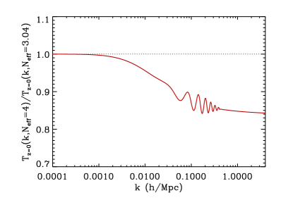
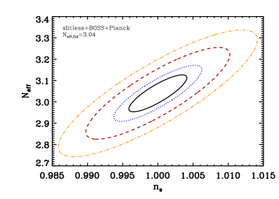
Interpreting the sign of the correlations is not so straightforward for the $N_{\rm eff}$–cosmology, since the number of relativistic species gives two opposite contributions to $P_{\rm obs}$, and the total sign of the correlation depends on the dominant one, for each single cosmological parameter. In fact, from the bottom-left panel of Fig. 2, it is clear that a larger $N_{\rm eff}$ value suppresses the transfer function $T(k)$ on scales $k\leq k_{\rm max}$. On the other hand, from Eq. (19) and Eq. (24), we see that a larger $N_{\rm eff}$ value also increases the Alcock-Paczynski prefactor in $P_{\rm obs}$. For what concerns the dark-energy parameters $\Omega_{de}$, $w_{0}$, $w_{a}$, and the dark-matter density $\Omega_{m}$, we find that the Alcock-Paczynski prefactor dominates, so that $N_{\rm eff}$ is positively correlated to $\Omega_{de}$ and $w_{a}$, and anti-correlated to $\Omega_{m}$ and $w_{0}$. In contrast, for the other parameters, the $T(k)$ suppression produces the larger effect and $N_{\rm eff}$ results to be anti-correlated to $\Omega_{b}$, and positively correlated to $h$ and $n_{s}$. See the last column in the upper panels of Tables 3-4 for the LSS alone case. The degree of the correlation $r$ is stable against the spectroscopic strategy adopted and is very large in the $n_{s}$-$N_{\rm eff}$ case, being $r\sim 0.8$ with and without Planck priors. For the remaining cosmological parameters, all the correlations are reduced when CMB information are added, except for the covariance $N_{\rm eff}$-$\Omega_{de}$, as happens also for the $M_{\nu}$–cosmology. To summarise, after the inclusion of Planck priors, the remaining dominant correlations among $N_{\rm eff}$ and the other cosmological parameters are $N_{\rm eff}$-$n_{s}$, $N_{\rm eff}$-$\Omega_{de}$, and $N_{\rm eff}$-$h$.

5.4 $N_{\rm eff}$–cosmology: Forecasted errors

The 1–$\sigma$ errors of the parameters are shown in the last column of Tables 1-2. Also in this case, compared to the slitless spectroscopy, the multi-slit spectroscopy is able to reduce the $N_{\rm eff}$ errors by $\sim$30% when LSS alone are used. When Planck priors are added, we find a 1–$\sigma$ error on $N_{\rm eff}$ of $\sim 0.08$, with a difference of only $6\%$ between the two spectroscopy strategies, again in favour of the multi-slit one.

5.5 Constraints on neutrino properties in the context of dark energy surveys

The main science goal of the galaxy surveys considered in this work is to constrain dark energy. Considering neutrinos properties might degrade the dark energy constraints (because of the introduction of extra parameters in the model), or it may be that such surveys are not optimised (e.g., in their redshift coverage) to measure neutrino properties and thus perform sub-optimally for these parameters.

We find that, depending on the fiducial $M_{\nu}$ value, the total CMB+LSS dark-energy FoM decreases only by $\sim 15\%-25\%$ with respect to the FoM obtained if neutrinos are assumed to be massless, and that, for the $N_{\rm eff}$–cosmology, the total CMB+LSS dark-energy FoM decreases only by $\sim 5\%$ with respect to the FoM obtained by holding $N_{\rm eff}$ fixed. This means that the “$P(k)$–method marginalised over growth–information” is quite robust in constraining the dark-energy equation of state.

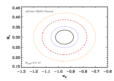
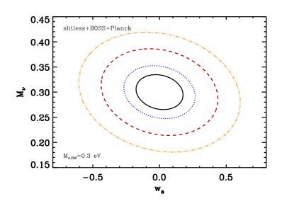
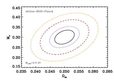
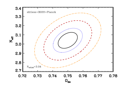
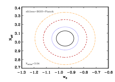
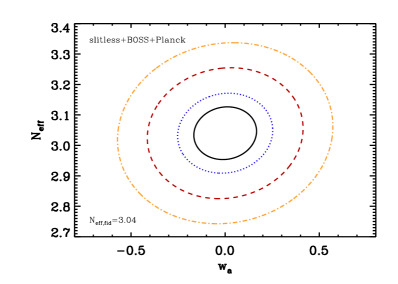
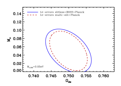
In Figs. 3-4 we show the jointly 2-parameter projected 68$\%$ C.L., 95.4$\%$ C.L. and 99.73$\%$ C.L. contours in the $\zeta$-$q_{\alpha}$ sub-space, where $\zeta=M_{\nu},N_{\rm eff}$ and $q_{\alpha}=\Omega_{de},w_{0},w_{a},\Omega_{m},n_{s}$, in the case of the slitless survey in combination with BOSS and Planck priors, for the $N_{\rm eff}$– and $M_{\nu}(=0.3$ eV)–cosmologies. The black solid lines show the 1-parameter confidence levels at 1–$\sigma$. The orientation of the ellipses reflects the correlations among the parameters shown in the lower panels of Tables 3-4.

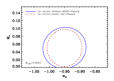
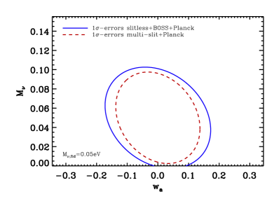
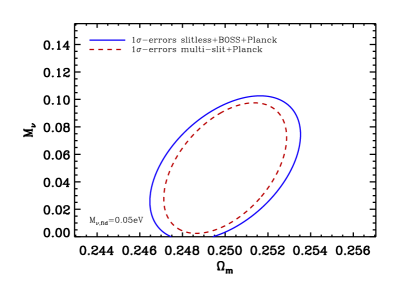
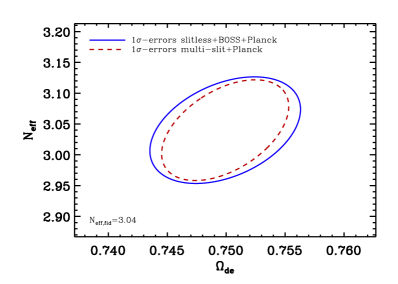
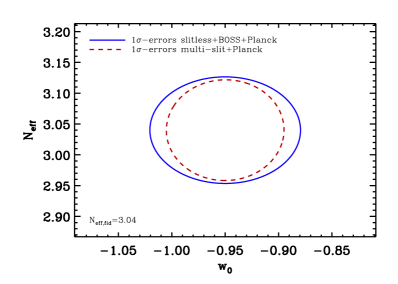
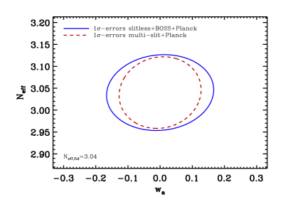
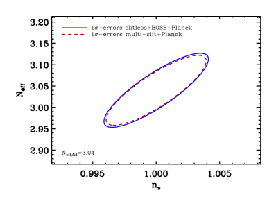
Moreover, for a visual comparison of the constraints obtained with the two spectroscopic strategies, in Figs. 5-6 we show the 1-parameter confidence levels at 1-$\sigma$ in the $\zeta$-$q_{\alpha}$ sub-space for the combinations slitless+BOSS+Planck and multi-slit+Planck, respectively.

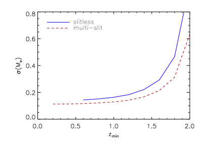
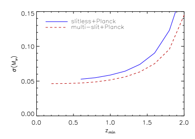
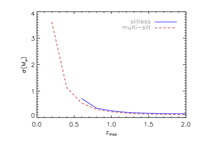
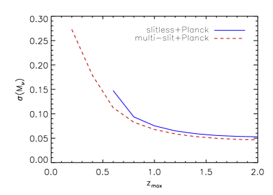
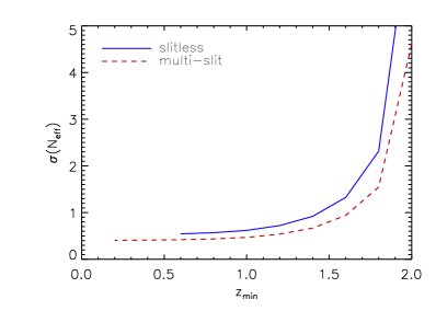
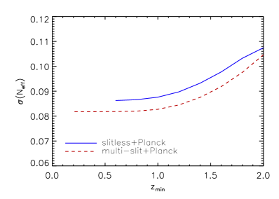
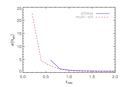
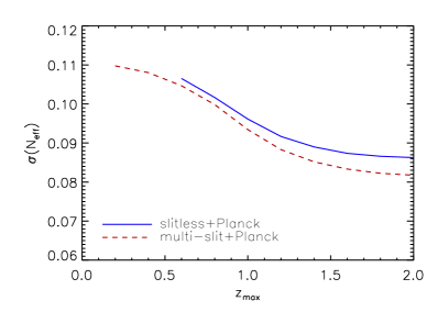
Finally, we consider the fiducial cosmology with $M_{\nu}|_{\rm fid}=0.05$ eV and, in the top panels of Fig. 7, we show the $M_{\nu}$–errors as functions of the minimum redshift $z_{min}$ of the surveys, with and without Planck priors. We fix the maximum redshift $z_{max}=2.1$ for both the spectroscopic strategies, while the lowest minimum redshifts are given by $z_{min}=0.5$ and $z_{min}=0.1$ for the slitless and multi-slit spectroscopies, respectively. In the bottom panels of Fig. 7, we show the $M_{\nu}$–errors as functions of the maximum redshift $z_{max}$ of the surveys, where we have fixed the minimum redshifts $z_{min}=0.5$ and $z_{min}=0.1$ for the slitless and multi-slit spectroscopies, respectively. For the slitless case, we have verified that extending the minimum redshift to $z_{min}=0.1$ changes the neutrino constraints by $\sim$0.8% only. We make the same analysis for the $N_{\rm eff}$–errors and the corresponding trends are shown in Fig. 8.

Note that concerning the possible degeneracies with the dark-energy parameters, we find that the major covariance is with $\Omega_{de}$, rather than with the dark energy equation of state parameters $w_{0}$ and $w_{a}$, and that extending the redshift range of the surveys considered would not reduce drastically the forecasted errors.

5.6 The effects of growth inclusion and random peculiar velocities on neutrino mass constraints

It is well known that galaxy peculiar velocities produce redshift-space distortions (RDS), which can be exploited by a large deep redshift survey to measure the growth rate of density fluctuations $f_{g}$, within the same redshift bins in which $H(z)$ is estimated via BAO. In particular, RDS allow to constrain $f_{g}$ times the normalisation of the power spectrum, i.e. $f_{g}\sigma_{8}$. In order to include growth information in our Fisher matrix analysis, following Ref. [65], we rewrite Eq. (3) as

$$P_{obs}(k_{{\rm ref}\perp},k_{{\rm ref}\parallel},z)=\frac{D_{A}(z)_{\rm ref}^{2}H(z)}{D_{A}(z)^{2}H(z)_{\rm ref}}\left[\sigma_{8g}(z)+f_{g}(z,k)\sigma_{8}(z)\frac{k_{{\rm ref}\parallel}^{2}}{k_{{\rm ref}\perp}^{2}+k_{{\rm ref}\parallel}^{2}}\right]^{2}\times C(k,z)+P_{shot},$$ (25)

where $C(k,z)\equiv P_{\rm matter}(k,z)/\sigma^{2}_{8}(z)$, and $\sigma_{8g}(z)=b(z)\sigma_{8}(z)$. We refer to this as the “full $P(k)$–method, with growth–information included”. Let us stress that we model RDS as an additive component, using as free parameters $(b\sigma_{8},f_{g}\sigma_{8})$. $f_{g}\sigma_{8}$ can be measured without knowing the bias $b$ or the amplitude of the matter fluctuations $\sigma_{8}$; therefore this parameter choice reduces possible systematic errors due to estimates of the bias [76].

While, for large separations, galaxy peculiar velocities give information on the growth of structures, on small scales random peculiar velocities cause the so-called Fingers of God (FoG), stretching compact structures along the line-of-sight [76, 77]. Although, on the scales of interest in this work, this effect is expected to be moderate [78, 79], we now include it in the Fisher analysis by introducing a Gaussian distribution for the pairwise velocity dispersion in configuration space, which produces a Gaussian damping $e^{-k^{2}\mu^{2}\sigma_{v}^{2}}$ of the observed galaxy power spectrum $P_{obs}$. This effect is degenerate with possible inaccuracies $\sigma_{z}$ in the observed redshifts due to a line-of-sight smearing of the structures, so we absorb it in the Gaussian damping factor of Eq. (5).

For the sake of simplicity, we consider only the fiducial cosmology with $M_{\nu}=0.05$ eV. In fact, in this case, the scale dependence of the growth rate $f_{g}$ due to free-streaming massive neutrinos can be assumed to be negligible. This is evident from the bottom-right panel of Fig. 2, where we show the scale dependence correction to $f_{g}$ for $M_{\nu}=0.05$ eV, given by the function $\mu(k,f_{\nu},\Omega_{de})\equiv f_{g}(M_{\nu}\neq 0)/f_{g}(M_{\nu}=0)$, where $f_{\nu}=\Omega_{\nu}/\Omega_{m}$, introduced by Ref. [11] in their Eqs. (16)-(17). In this case the growth suppression is only of the order of $0.2\%$, affecting scales $k>0.1\,h$/Mpc.

Under these assumptions, when we include the effect of FoG in the Fisher analysis, we consider also $\sigma_{v}(z_{i})$ as a scale independent variable, which is treated as a nuisance parameter to be marginalised over in each redshift bin, together with {$\sigma_{8g}(z_{i})$, $P_{shot}^{i}$}, and we project the errors on {$H(z_{i})$, $D_{A}(z_{i})$, $f_{g}(z_{i})\sigma_{8}(z_{i})$, $\omega_{m}$, $\omega_{b}$, $\zeta$, $n_{s}$, $h$} into the final set of cosmological parameters {$\Omega_{m}$, $\Omega_{de}$, $\Omega_{b}$, $h$, $\zeta$, $w_{0}$, $w_{a}$, $n_{s}$, $\sigma_{8}$}. This parameter set differs from Eq. (18) only for the substitution $\Delta^{2}_{\cal R}(k_{0})\rightarrow\sigma_{8}$, whose fiducial value is fixed by $\Delta^{2}_{\cal R}(k_{0})=2.45\times 10^{-9}$ and the other parameters of the $M_{\nu}|_{\rm fid}(=0.05{\rm eV})$–cosmology described in §4 . We refer to this as the “full $P(k)$–method, with FoG and growth–information included”.

In what follows we compare the $M_{\nu}$ constraints obtained by the three $P(k)$–methods considered in this work, for the fiducial cosmology with $M_{\nu}|_{\rm fid}=0.05$ eV.

5.6.1 Growth inclusion effects

We find that neutrino mass errors are quite stable at $\sigma(M_{\nu})=0.05$ eV, against the adopted method (whether growth–information are included or marginalised over), and decrease only by $10\%$–$20\%$ when $f_{g}\sigma_{8}$ measurements are included. We can understand this result as follows. $\Omega_{\nu}$ affects the shape of the power spectrum, i.e. enters the transfer function $T(k,z)$, which is sampled on a very large range of scales, including the $P(k)$ turnover scale, by the nearly full-sky surveys under consideration. On the other hand, $f_{g}$ is only slightly dependent on $M_{\nu}$ for $M_{\nu}|_{\rm fid}=0.05$ eV (see the bottom-right panel of Fig. 2). Consequently, the effect on the observed power spectrum shape dominates over the information extracted by measurements of $f_{g}\sigma_{8}$. This quantity, in turn, generates new correlations with $M_{\nu}$ via the $\sigma_{8}$-term, which now we constrain simultaneously with the other cosmological parameters, and which actually is anti-correlated with $M_{\nu}$ [80].

On the other hand, if we suppose that early dark-energy is negligible, the dark-energy parameters $\Omega_{de}$, $w_{0}$ and $w_{a}$ do not enter the transfer function, and consequently growth information have relatively more weight when added to constraints from $H(z)$ and $D_{A}(z)$ alone.

As a result, the $M_{\nu}$–errors are quite insensitive to growth inclusion, hence almost independent of the adopted $P(k)$–method. This is in contrast to the dark-energy parameter constraints (see e.g. Ref. [11]). In fact, we find that, with respect to the “full $P(k)$–method, marginalised over growth–information”, the “full $P(k)$–method, with growth–information included” is able to increase the dark-energy FoM by $\sim 50$% and $\sim 60$% for the slitless and multi-slit strategies, respectively, from both LSS data alone and in combination with Planck priors, when massive neutrinos are assumed in the fiducial cosmology.

To summarise, we find that, due to the slight dependence of $f_{g}$ on $M_{\nu}$ when $M_{\nu}|_{\rm fid}=0.05$ eV, and due to the further degeneracy with $\sigma_{8}$ (correlated also with the dark-energy parameters), we do not find a total effective gain on the accuracy of $M_{\nu}$ measurements, when growth-information are added. On the other hand, the value of the dark-energy FoM does increase when growth-information are included, even if it decreases by a factor $\sim 2-3$ with respect to cosmologies where neutrinos are assumed to be massless, due to the correlation among $M_{\nu}$ and the dark-energy parameters. As confirmation of this degeneracy, we find that, when growth-information are added and if the dark-energy parameters $\Omega_{de}$, $w_{0}$, $w_{a}$ are held fixed to their fiducial values, the errors $\sigma({M_{\nu}})$ decrease to $0.027$ eV and $0.025$ eV, for the slitless and multi-slit spectroscopies combined with Planck, respectively.

5.6.2 Incoherent velocity inclusion effects

We expect that dark-energy parameter errors are somewhat sensitive to FoG effects. This can be understood in terms of correlation functions in the redshift-space; the stretching effect due to random peculiar velocities contrasts the flattening effect due to large-scale bulk velocities. Consequently, these two competing effects act along opposite directions on the dark-energy parameter constraints.

We find that the dark-energy FoM obtained with the “full $P(k)$–method, with FoG and growth–information included” result to be FoM${}^{\rm LSS}=51,\,95$ and FoM${}^{\rm LSS+CMB}=268,\,391$, for the slitless and multi-slit spectroscopies respectively, i.e. very similar to the FoMs obtained from the “full $P(k)$–method, marginalised over growth–information”, as shown in Tables 1-2, which therefore can be considered a more stable approach against galaxy peculiar velocity uncertainties.

On the other hand, the neutrino mass errors are expected to be almost stable at $\sigma({M_{\nu}})=0.05$ when FoGs effects are taken into account by marginalising over $\sigma_{v}(z)$, increasing only by $10\%$–$14\%$ with respect to the “full $P(k)$–method, marginalised over growth–information”. Moreover, in this case, if the dark-energy parameters $\Omega_{de}$, $w_{0}$, $w_{a}$ are held fixed to their fiducial values, the errors $\sigma({M_{\nu}})$ become $0.029$–$0.028$ eV, for the slitless and multi-slit spectroscopies combined with Planck, respectively. In other words, we get errors which are only $\sim$11% larger than the ones obtained without marginalising over $\sigma_{v}(z)$ under the same assumptions on $\Omega_{de}$, $w_{0}$, and $w_{a}$, as described in §5.6.1.

5.7 Systematic effects, non-linearities and bias

Fisher-matrix based forecasts are not particularly well suited to quantify systematic effects. The errors reported so far are statistical errors, which are meaningful only as long as they dominate over systematic errors. It is therefore important to consider sources of systematics and their possible effects on the recovered parameters. Possible sources of systematic errors of major concern are the effect of non-linearities and the effects of galaxy bias. In our analysis so far we have used the linear theory matter power spectrum and applied scale-independent bias to it.

The description of non-linearities in the matter power spectrum in the presence of massive neutrinos is a relatively new subject. It has been addressed in several different ways: Refs. [81, 75, 82, 83] use perturbation theory, Ref. [84] used the time-RG flow approach and Refs. [85, 86, 88, 13] used different schemes of N-body simulations. From the above references it is clear that the effect of massive neutrinos on the matter power spectrum in the non-linear regime must be explored via N-body simulations to encompass all the relevant effects. Different simulations schemes and approximations agree already at or below the % level (for neutrino masses allowed by current observations and $k<1$ Mpc/$h$) indicating that non-linear effects on the matter power spectrum can in the future be modelled to the required accuracy.

On the scales considered in this work the effects of non-linearities are small and statistical–errors could be further reduced considering smaller scales. As shown in [75], the effect of non linearities does not erase or reduce the effect of massive neutrinos. In fact, by comparing Fig. 4 of [75] and e.g., Fig. 4 of [86], it is apparent that the difference between the massless and massive neutrino case is enhanced by non-linearities. Thus while it will be mandatory to include non-linearities in the actual data analysis, the forecasted errors are not made artificially smaller by using the linear matter power spectrum to compute our Fisher matrices.

Pushing to smaller scales however would worsen the systematic effect of scale-dependent and/or non-linear bias. Here we have made the simplifying assumption that bias is scale-independent up to $k_{max}$ but the redshift dependence is not known and is marginalised over. Bias is known to be scale-independent on large, linear scales but to become non-linear and scale-dependent for small scales and/or for very massive halos. A scale-dependence of bias may mimic in part the effect of massive neutrinos. The scale-dependence of bias however is expected not to have the same redshift dependence as massive neutrino effects, thus offering the possibility to break a possible degeneracy. A scale-dependence of bias may cancel in part the effect of massive neutrinos. It arises because halos, especially massive or rare ones, are non-linearly biased with respect to the dark matter. Scale-dependent bias (at least for dark matter halos hosting galaxies) is found first to increase with increasing $|k|$ then decrease, but the bias of the galaxies hosted in the dark halos may be more complicated. This will be an important limitation in any practical application especially if we want to include mildly non-linear scales. There are, however, several possibilities to control or quantify systematics introduced by bias. In fact, the bias behaviour varies for differently selected objects (different colour or different brightness): splitting the sample in differently-biased tracers will thus help disentangle the systematic effect from the cosmological signal (approach similar to that of e.g.,[69]). Finally on large, linear scales, the neutrino mass splitting leaves a specific signature on the shape of the power spectrum that can also be used as a cross check of the $M_{\nu}$ signal as illustrated in Ref. [87]. A more quantitative investigation of scale-dependent bias is beyond the scope of this paper, but we plan to study this important issue as more data and simulations become available.

Table 5: $\sigma(M_{\nu})$ and $\sigma(N_{\rm eff})$ marginalised errors from LSS+CMB

			General cosmology
fiducial$\to$	$M_{\nu}$=0.3 eVa	$M_{\nu}$=0.2 eVa	$M_{\nu}$=0.125 eVb	$M_{\nu}$=0.125 eVc	$M_{\nu}$=0.05 eVb	$N_{\rm eff}$=3.04d
slitless+BOSS+Planck	$0.035$	$0.043$	$0.031$	$0.044$	$0.053$	$0.086$
multi-slit+Planck	$0.030$	$0.038$	$0.027$	$0.039$	$0.046$	$0.082$
			$\Lambda$CDM cosmology
slitless+BOSS+Planck	$0.017$	$0.019$	$0.017$	$0.021$	$0.021$	$0.023$
multi-slit+Planck	$0.015$	$0.016$	$0.014$	$0.018$	$0.018$	$0.019$

^afor degenerate spectrum: $m_{1}\approx m_{2}\approx m_{3}$; ^bfor normal hierarchy: $m_{3}\neq 0$, $m_{1}\approx m_{2}\approx 0$
^cfor inverted hierarchy: $m_{1}\approx m_{2}$, $m_{3}\approx 0$; ^dfiducial cosmology with massless neutrinos

6 Conclusions

In this work we have forecasted errors on the total neutrino mass $M_{\nu}$ and the effective number of relativistic species $N_{\rm eff}$, by combining Planck priors with future data from space-based spectroscopic galaxy redshift surveys in the near-IR. We have considered two survey strategies based on slitless and multi-slit spectroscopies. The assumed set of cosmological parameters is very general and takes into account a time-varying dark-energy equation of state, as well as a non-vanishing spatial curvature of the Universe. We exploited information from the galaxy power spectrum shape and BAO positions, marginalising over galaxy bias; thus our findings do not depend on bias measurement accuracy (as long as, on the large scales considered, bias is scale independent or its scale dependence is known), or modelling of the redshift dependence of bias [21].

The 1–$\sigma$ errors are shown in Tables 1-2, and the correlation coefficients in Tables 3-4. In Figs. 3-5 we show the joint 2-parameter confidence levels.

Regarding $M_{\nu}$–errors, we find that the multi-slit spectroscopy is able to reduce the neutrino mass errors of about 20%-30% compared to the slitless spectroscopy, depending on the fiducial total neutrino mass, if LSS data alone are used. When Planck priors are added, the 1–$\sigma$ errors on $M_{\nu}$ are in the range $0.03-0.05$ eV, depending on the fiducial neutrino mass, with an average difference of 15% between the two spectroscopic strategies, favouring the multi-slit spectroscopy.

Moreover, depending on the fiducial $M_{\nu}$–value, the total CMB+LSS dark-energy FoM, with growth–information marginalised over, decreases only by $\sim 15\%-25\%$ with respect to the value obtained if neutrinos are assumed to be massless (or their mass is assumed to be perfectly known), meaning that the “$P(k)$–method marginalised over growth–information” is quite robust to assumptions about model cosmology when constraining the dark-energy equation of state. The situation is different when we include growth-information, since in this case the value of the dark-energy FoM decreases by a factor $\sim 2-3$ with respect to cosmologies that assume massless neutrinos.

Considering the fiducial cosmology with $M_{\nu}|_{\rm fid}=0.05$ eV, in §5.6 we checked the stability of $M_{\nu}$–errors to the inclusion of growth–information and peculiar velocity uncertainties. We compared the following approaches: the “full $P(k)$–method, marginalised over growth–information”, the “full $P(k)$–method, with growth–information included”, and “full $P(k)$–method, with FoG and growth–information included”. We found that $M_{\nu}$–errors are quite stable at $\sigma(M_{\nu})=0.05$ eV, against the adopted method. This result is as expected, if we consider that, unlike dark energy parameters, $M_{\nu}$ affects the shape of the power spectrum via a redshift-dependent transfer function $T(k,z)$, which is sampled on a very large range of scales including the $P(k)$ turnover scale, therefore this effect dominates over the information extracted from measurements of $f_{g}\sigma_{8}$.

Regarding $N_{\rm eff}$–errors, again we find that, compared to the slitless spectroscopy, the multi-slit spectroscopy is able to reduce the $N_{\rm eff}$–errors by $\sim$30% when LSS alone are used. When Planck priors are added, we find $\sigma(N_{\rm eff})\sim 0.08$, with only a $6\%$ difference between the two spectroscopy strategies, again in favour of the multi-slit one. The total CMB+LSS dark-energy FoM decreases only by $\sim 5\%$ with respect to the value obtained holding $N_{\rm eff}$ fixed at its fiducial value, meaning that also in this case the “$P(k)$–method marginalised over growth–information” is not too sensitive to assumptions about model cosmology when constraining the dark-energy equation of state.

Finally, in Table 5 we summarise the dependence of the $M_{\nu}$– and $N_{\rm eff}$–errors on the model cosmology, for the two spectroscopic strategies combined with Planck. We conclude that, if $M_{\nu}$ is $>0.1$ eV, these surveys will be able to determine the neutrino mass scale independently of the model cosmology assumed. If $M_{\nu}$ is $<0.1$ eV, the sum of neutrino masses, and in particular the minimum neutrino mass required by neutrino oscillations, can be measured in the context of a $\Lambda$CDM model.

This means that future spectroscopic galaxy surveys, such as Euclid or SPACE, JEDI, and possibly WFIRST in the future, will be able to cover the entire parameter space for neutrino mass allowed by oscillations experiments

Moreover, as summarised in Fig. 1, they will be competitive with future 3D cosmic shear photometric surveys, which, in combination with Planck priors, will give similar constraints on $M_{\nu}$ and $N_{\rm eff}$ [9]. Since, these two kinds of LSS probe are affected by different systematics, their constraints on neutrino masses and relativistic degrees of freedom will provide a consistency check of the two independent measurement methods.

We conclude that future nearly all-sky spectroscopic galaxy surveys will detect the cosmic neutrino background at high statistical significance, and provide a measurement of the neutrino mass scale. This will provide an important confirmation of our model for the early Universe, and crucial insights into neutrino properties, highly complementary to future particle physics experiments.

Appendix A Planck priors

In this work we use the Planck mission parameter constraints as CMB priors, by estimating the cosmological parameter errors via measurements of the temperature and polarisation power spectra. As CMB anisotropies, with the exception of the integrated Sachs-Wolfe effect, are not able to constrain the equation of state of dark-energy $(w_{0},w_{a})$, we follow the prescription laid out by DETF [72].

We do not include any B-mode in our forecasts and assume no tensor mode contribution to the power spectra. We use the 100 GHz, 143 GHz, and 217 GHz channels as science channels. These channels have a beam of $\theta_{\rm fwhm}=9.5^{\prime}$, $\theta_{\rm fwhm}=7.1^{\prime}$, and $\theta_{\rm fwhm}=5^{\prime}$, respectively, and sensitivities of $\sigma_{T}=2.5\mu K/K$, $\sigma_{T}=2.2\mu K/K$, $\sigma_{T}=4.8\mu K/K$ for temperature, and $\sigma_{P}=4\mu K/K$, $\sigma_{P}=4.2\mu K/K$, $\sigma_{P}=9.8\mu K/K$ for polarisation, respectively. We take $f_{\rm sky}=0.80$ as the sky fraction in order to account for galactic obstruction, and use a minimum $\ell$-mode $\ell_{\rm min}=30$ in order to avoid problems with polarisation foregrounds and not to include information from the late Integrated Sachs-Wolfe effect, which depends on the specific dark-energy model. We discard temperature and polarisation data at $\ell>2000$ to reduce sensitivity to contributions from patchy reionisation and point source contamination (see [72] and references therein).

We assume a $\Lambda$CDM fiducial cosmology, and choose the following set of parameters to describe the temperature and polarisation power spectra $\vec{\theta}=(\omega_{m},\omega_{b},\zeta,100\times\theta_{S},\ln(10^{10}\Delta^{2}_{\cal R}(k_{0})),n_{S},\tau)$, where $\theta_{S}$ is the angular size of the sound horizon at last scattering, and $\tau$ is the optical depth due to reionisation. Note that a different parameter set is assumed in [89].

The Fisher matrix for CMB power spectrum is given by [90, 91]:

$$F_{ij}^{CMB}=\sum_{l}\sum_{X,Y}\frac{\partial C_{X,l}}{\partial\theta_{i}}\mathrm{COV^{-1}_{XY}}\frac{\partial C_{Y,l}}{\partial\theta_{j}},$$ (26)

where $\theta_{i}$ are the parameters to constrain, $C_{X,l}$ is the harmonic power spectrum for the temperature-temperature ($X\equiv TT$), temperature-E-polarisation ($X\equiv TE$) and the E-polarisation-E-polarisation ($X\equiv EE$) power spectrum. The covariance $\rm{COV}^{-1}_{XY}$ of the errors for the various power spectra is given by the fourth moment of the distribution, which under Gaussian assumptions is entirely given in terms of the $C_{X,l}$ with

$${\rm COV}_{T,T} = f_{\ell}\left(C_{T,l}+W_{T}^{-1}B_{l}^{-2}\right)^{2}$$ (27)

$${\rm COV}_{E,E} = f_{\ell}\left(C_{E,l}+W_{P}^{-1}B_{l}^{-2}\right)^{2}$$ (28)

$${\rm COV}_{TE,TE} = f_{\ell}\Big{[}C_{TE,l}^{2}+$$

$$\left(C_{T,l}+W_{T}^{-1}B_{l}^{-2}\right)\left(C_{E,l}+W_{P}^{-1}B_{l}^{-2}\right)\Big{]}$$

$${\rm COV}_{T,E} = f_{\ell}C_{TE,l}^{2}$$ (30)

$${\rm COV}_{T,TE} = f_{\ell}C_{TE,l}\left(C_{T,l}+W_{T}^{-1}B_{l}^{-2}\right)$$ (31)

$${\rm COV}_{E,TE} = f_{\ell}C_{TE,l}\left(C_{E,l}+W_{P}^{-1}B_{l}^{-2}\right)\;,$$ (32)

where $f_{\ell}=\frac{2}{(2\ell+1)f_{\rm sky}}$, $W_{T,P}=\sum_{c}W^{c}_{T,P}$, $W^{c}_{T,P}=(\sigma^{c}_{T,P}\theta^{c}_{\rm fwhm})^{-2}$ being the weight per solid angle for temperature and polarisation respectively, with a 1–$\sigma$ sensitivity per pixel of $\sigma^{c}_{T,P}$ and a beam of $\theta^{c}_{\rm fwhm}$ extent, for each frequency channel $c$. The beam window function is given in terms of the full width half maximum (fwhm) beam width by $B_{\ell}^{2}=\sum_{c}(B^{c}_{\ell})^{2}W^{c}_{T,P}/W_{T,P}$, where $(B^{c}_{\ell})^{2}=\exp\left(-\ell(\ell+1)/(l^{c}_{s})^{2}\right)$, $l^{c}_{s}=(\theta^{c}_{\rm fwhm})^{-1}\sqrt{(}8\ln 2)$ and $f_{\rm sky}$ is the sky fraction [92].

We then calculate the Planck CMB Fisher matrix with the help of the publicly available CAMB code [93]. Finally, we transform the Planck Fisher matrix for the DETF parameter set to the final parameter sets $\bf q$ considered in this work (see §4 and §5.6), using the transformation

$$F_{\alpha\beta}^{\rm CMB}=\sum_{ij}\frac{\partial\theta_{i}}{\partial q_{\alpha}}\,F_{ij}^{\rm CMB}\,\frac{\partial\theta_{j}}{\partial q_{\beta}}.$$ (33)

References

- [1] Lesgourgues, J. & Pastor, S. 2006,Physics Reports, 429, 307
- [2] V. M. Lobashev 2003, Nucl. Phys. A, 719, 153.
- [3] C. Kraus et al. 2005, Eur. Phys. J. C, 40, 447.
- [4] T. Thummler, f. t. K. Collaboration, \arXivid1012.2282
- [5] Komatsu, E., et al. 2010, \arXivid1001.4538
- [6] Namikawa, T., Saito, S., & Atsushi, T. 2009, \arXivid1009.3204
- [7] Lesgourgues, J., Perotto, L., Pastor, S., & Piat, M. 2006, Phys. Rev. D, 73, 045021
- [8] Perotto, L., Lesgourgues, J., Hannestad, S., Tu, H., & Y Y Wong, Y. 2006, Journal of Cosmology and Astro-Particle Physics, 10, 13
- [9] Kitching, T. D., Heavens, A. F., Verde, L., Serra, P., & Melchiorri, A. 2008, Phys. Rev. D, 77, 103008
- [10] Hu, W., Eisenstein, D. J., & Tegmark, M. 1998, Phys. Rev. Lett., 80, 5255
- [11] Kiakotou, A., Elgaroy, O., & Lahav, O. 2008, Phys. Rev. D, 77, 063005
- [12] Brandbyge, J., Hannestad, S., Haugbølle, T., Wong, Y. 2010, Journal of Cosmology and Astro-Particle Physics, 09, 014
- [13] Viel, M., Haehnelt, M. G., & Springel, V. 2010, Journal of Cosmology and Astro-Particle Physics, 06, 015
- [14] Reid, B. A., Verde, L., Jimenez, R., & Mena, O. 2010, Journal of Cosmology and Astro-Particle Physics, 1, 3
- [15] Wang, S., Haiman, Z., Hu, W., Khoury, J., & May, M. 2005, Phys. Rev. Lett., 95, 011302
- [16] Thomas, S. A., Abdalla, F. B., & Lahav, O. 2009, Phys. Rev. Lett., 105, 031301
- [17] Gonzalez-Garcia, M. C., Maltoni, M., & Salvado, J. 2010, \arXivid1006.3795
- [18] Hannestad, S., & Wong, Y. Y. Y. 2007, Journal of Cosmology and Astro-Particle Physics, 7, 4
- [19] Hannestad, S. 2010, Prog. Part. Nucl. Phys., 65, 185
- [20] LSST Science Collaborations, et al. 2009, \arXivid0912.0201
- [21] Lahav, O., Kiakotou, A., Abdalla, F. B., & Blake, C. 2010, Mont. Not. Roy. Astron. Soc., 405, 168
- [22] A. G. Cocco, G. Mangano and M. Messina 2007, Journal of Cosmology and Astro-Particle Physics, 0706, 015
- [23] Jimenez, R., Kitching, T., Peña-Garay, C., & Verde, L. 2010, Journal of Cosmology and Astro-Particle Physics, 5, 35
- [24] Lesgourgues, J., Pastor, S., & Perotto, L. 2004, Phys. Rev. D, 70, 045016
- [25] Melchiorri, A., Mena, O., Palomares-Ruiz, S., Pascoli, S., Slosar, A., & Sorel, M., Journal of Cosmology and Astro-Particle Physics , 1, 36 (2009)
- [26] A. A. Aguilar-Arevalo et al. 2007, Phys. Rev. Lett., 98, 231801
- [27] Mangano, G., Melchiorri, A., Mena, O., Miele, G., and Slosar, A. 2007, Journal of Cosmology and Astro-Particle Physics, 0703, 006
- [28] Bonometto S., Pierpaoli E. 1998, New Astronomy, 3 , 391
- [29] Lopez R.E.,Dodelson S., Sherrer R.J., Turner M.S. 1998, Phys. Rev. Lett. 81, 3075
- [30] Hannestad S. 1998, Phys.Rev.Lett., 80, 4621
- [31] Kaplinghat M., Turner M.S., 2001, Phys. Rev. Lett., 86, 385
- [32] Bean R., Hansen S.H., Melchiorri A. 2001, Phys. Rev. D, 64, 103508
- [33] Davoudiasl,H. 2007, Phys. Rev. Lett., 99, 141301
- [34] Trotta, R. and Melchiorri, A. 2005, Phys. Rev. Lett., 95, 011305
- [35] De Bernardis, F., Melchiorri, A., Verde, L., & Jimenez, R. 2008, Journal of Cosmology and Astro-Particle Physics, 3, 20
- [36] Figueroa, D. G., Verde, L., & Jimenez, R. 2008, Journal of Cosmology and Astro-Particle Physics, 10, 38
- [37] Stern, D., Jimenez, R., Verde, L., Kamionkowski, M., & Stanford, S. A. 2010, Journal of Cosmology and Astro-Particle Physics, 2, 8
- [38] Wang, Y., et al., 2004, BAAS, v36, n5, 1560
- [39] Crotts, A. et al. 2005 \arXividastro-ph/0507043
- [40] Cheng, E., & Wang, Y. et al., 2006, Proc. of SPIE, Vol. 6265, 626529
- [41] Cimatti, A.; Robberto, M.; Baugh, C.; Beckwith, S. V. W.; Content, R.; Daddi, E.; De Lucia, G.; Garilli, B.; Guzzo, L.; Kauffmann, G.; Lehnert, M.; Maccagni, D.; Martínez-Sansigre, A.; Pasian, F.; Reid, I. N.; Rosati, P.; Salvaterra, R.; Stiavelli, M.; Wang, Y.; Osorio, M. Zapatero; the SPACE team, Experimental Astronomy, 23, 39 (2009)
- [42] Glazebrook, K., et al., 2005, New Astronomy Reviews, 49, 374
- [43] Laureijs, R. et al. 2009, “Euclid Assessment Study Report for the ESA Cosmic Visions”, \arXivid0912.0914
- [44] Gehrels, N., et al., Final Report of the Joint Dark Energy Mission Science Coordination Group, http://wfirst.gsfc.nasa.gov/science/SCG_Report.pdf
- [45] Vogeley, M. S. & Szalay, A. S. 1996 Astrophys. J., 465, 43
- [46] Tegmark, M., Taylor A., Heavens A. 1997, Astrophys. J., 480, 22
- [47] Jungman, G., Kamionkowski, M., Kosowsky, A., Spergel, D. 1996, Phys. Rev. D, 54, 1332
- [48] Fisher, R. 1935, J. Roy. Statist. Soc., 98, 35
- [49] Feldman, H., A., Kaiser, N., & Peacock, J., A. 1994, Astrophys. J., 426, 23
- [50] Seo, H., J., & Eisenstein, D., J. 2003, Astrophys. J., 598, 720
- [51] W. E. Ballinger, J. A. Peacock, and A. F. Heavens, Mon.Not.Roy.As.Soc. 282, 877 (1996), a
- [52] Seljak, U. 2000, Mont. Not. Roy. Astron. Soc., 318, 203
- [53] Kaiser, N. 1987, Mont. Not. Roy. Astron. Soc., 227, 1
- [54] Takada, M., Komatsu, E., Futamase, T. 2006, Phys. Rev. D, 73, 083520
- [55] Takada, M. 2006, Phys. Rev. D, 74, 043505
- [56] Eisenstein, D., J., & Hu, W. 1997, Astrophys. J., 511, 5
- [57] Linder, E. V. & Jenkins, A. 2003, Mont. Not. Roy. Astron. Soc., 346, 573
- [58] Lewis, A., Challinor, A., & Lasenby, A. 2000, Astrophys. J., 538, 473
- [59] Wang, Y. 2010, Mod. Phys. Lett. A, 25, 3093
- [60] Larson, D., et al. 2010, \arXivid1001.4635
- [61] Wang, Y. 2008, Journal of Cosmology and Astro-Particle Physics, 05, 021
- [62] Tegmark, S. 1997, Phys. Rev. Lett., 79, 3806
- [63] Wang, Y. 2006, Astrophys. J., 647, 1
- [64] Wang, Y. 2008, Phys. Rev. D, 77, 123525
- [65] Wang, Y., et al. 2010, Mont. Not. Roy. Astron. Soc., 409, 737
- [66] Geach, J. E.; Cimatti, A.; Percival, W.; Wang, Y.; Guzzo, L.; Zamorani, G.; Rosati, P.; Pozzetti, L.; Orsi, A.; Baugh, C. M.; Lacey, C. G.; Garilli, B.; Franzetti, P.; Walsh, J. R.; Kümmel, M., 2010, Mont. Not. Roy. Astron. Soc., 402, 1330
- [67] Orsi, Alvaro; Baugh, C. M.; Lacey, C. G.; Cimatti, A.; Wang, Y.; Zamorani, G., \arXivid0911.0669, Mont. Not. Roy. Astron. Soc., in press (2010)
- [68] Reid, B. A., et al., 2010, Mont. Not. Roy. Astron. Soc., 404, 60
- [69] Swanson, M. E. C., Percival, W. J., Lahav O. 2010, doi:10.1111/j.1365-2966.2010.17371.x, \arXivid1006.2825
- [70] Chevallier, M., & Polarski, D. 2001, Int. J. Mod. Phys. D, 10, 213
- [71] Linder, E.V., 2003, Phys. Rev. Lett., 90, 091301
- [72] Albrecht, A. et al. 2009, \arXivid0901.0721
- [73] Komatsu, E., et al. 2009, Astrophys. J. Suppl., 180, 330
- [74] Reid, B., A., Verde, L. Jimenez, R., Mena, O. 2010, J. Cosm. Astropart. Phys., 01, 003
- [75] Saito, S.,Takada, M., & Taruya, A. 2009, Phys. Rev. D, 80, 083528
- [76] Song, Y. S., & Percival, W. J. 2009, Journal of Cosmology and Astro-Particle Physics, 0910, 004
- [77] Scoccimarro, R. 2004, Phys.Rev. D, 70, 083007
- [78] Percival, W. J., & White, M. 2009, Journal of Cosmology and Astro-Particle Physics, 393, 297
- [79] Jennings E., Baugh, C. M., & Pascoli, S. 2010, \arXivid1011.2842
- [80] Marulli, F., Carbone, C., Viel, M., Moscardini, L., & Cimatti, A. 2011, \arXivid1103.0278.
- [81] Y. Y. Y. Wong 2008, Journal of Cosmology and Astro-Particle Physics, 0810, 035
- [82] Saito, S., Takada, M., & Taruya, A. 2008, Phys. Rev. Lett., 100, 191301
- [83] Saito, S., Takada, M., & Taruya, A. \arXivid1006.4845
- [84] Lesgourgues, J., Matarrese, S., Pietroni, M., & Riotto, A. 2009, Journal of Cosmology and Astro-Particle Physics, 6, 17
- [85] Brandbyge, J., Hannestad, S., Haugbølle, T., & Thomsen, B. 2008, Journal of Cosmology and Astro-Particle Physics, 8, 20
- [86] Brandbyge, J., & Hannestad, S. 2009, Journal of Cosmology and Astro-Particle Physics, 5, 2
- [87] DePutter , R., et al. 2010, in prep.
- [88] Brandbyge, J., & Hannestad, S. 2010, Journal of Cosmology and Astro-Particle Physics, 1, 21
- [89] Mukherjee, P., Kunz, M., Parkinson, D., & Wang, Y., 2008, Phys.Rev. D, 78, 083529
- [90] Zaldarriaga M., Seljak U., 1997, PRD, 55, 1830
- [91] Zaldarriaga M., Spergel D. N., Seljak U., 1997, APJ, 488, 1
- [92] Bond, J. R., Efstathiou, G., & Tegmark, M. 1997 Mont. Not. Roy. Astron. Soc., 291, L33
- [93] Lewis, A., Challinor, A., & Lasenby, A. 2000, Astrophys. J., 538, 473