The Fast Linear Accelerator Modeling Engine for FRIB Online Model Service

Abstract

Commissioning of a large accelerator facility like FRIB needs support from an online beam dynamics model. Considering the new physics challenges of FRIB such as modeling of non-axisymmetric superconducting RF cavities and multi-charge state acceleration, there is no readily available online beam tuning code. The design code of FRIB super-conducting linac, IMPACT-Z, is not suitable for online tuning because of its code design and running speed. Therefore, the Fast Linear Accelerator Modeling Engine (FLAME), specifically designed to fulfill FRIB’s online modeling challenges, is proposed. The physics model of FLAME, especially its novel way of modeling non-axisymmetric superconducting RF cavities using a multipole expansion based thin-lens kick model, is discussed in detail, and the benchmark results against FRIB design code is presented, after which the software design strategy of FLAME and its execution speed is presented.

I INTRODUCTION

The Facility for Rare Isotope Beams (FRIB) is a new national user facility for nuclear science co-funded by the Department of Energy and Michigan State University (MSU), whose driver linac is designed to accelerate all stable ions to on-target energy larger than 200 MeV/u and power up to 400 kW. The FRIB driver linac consists of a front-end section where ions are generated and accelerated to 0.5 MeV/u, three linac segments with super-conducting Radio-frequency (RF) cavities where heavy ions gain most of their kinetic energy, two folding segments to confine the footprint and facilitate charge selection, and a beam delivery system to transport the beam to the target Wei et al. (2013, 2012). To commission and support daily operation of such a complex driver linac with thousands of tunable components can be quite a challenging endeavor, and an online model is essential to handle this task.

Due to the special modeling challenges, especially non-axisymmetric superconducting RF cavities Facco and Zvyagintsev (2011); Cavenago (1992) and multi-charge state acceleration Betz (1972), there is no readily available online physics model which can handle all the FRIB modeling challenges. And the design model of the FRIB super-conducting linac, IMPACT-Z Qiang et al. (1999), is only utilized for off-line use. In particular, it is not fast enough for online tuning. Therefore, a physics model specially designed for online purpose while covering all special FRIB modeling challenges with satisfactory execution speed is desired.

The Fast Linear Accelerator Modeling Engine (FLAME) is a novel beam envelope tracking code providing solutions to FRIB-specific challenges of modeling non-axisymmetric superconducting RF cavities and multi-charge state acceleration with control room quality. FLAME also implements matrix models for other major beam lattice elements of FRIB such as solenoid, magnetic and electrostatic quadrupole, magnetic and electrostatic dipole, and charge stripper. Modeling of element misalignment is also implemented. In the first section of this paper, the physics modeling strategy is discussed. Then, the code structure design and python interface of FLAME are discussed. Finally, calculation results of FLAME are benchmarked against FRIB design code, and execution speed of FLAME is also presented.

II Beam Dynamics Model for FLAME

The design code for FRIB super-conducting linac, IMPACT-Z, is a Particle-In-Cell (PIC) code. It is precise, but slow when considering online beam tuning applications. The often used online code, OpenXAL Pelaia et al. (2015) for example, is based on the beam envelope formalism. However, OpenXAL lacks some important features which are essential for correctly modeling FRIB. FLAME is a new online code specially designed to cover all FRIB modeling challenges. The first part of the paper describes the physics models for FLAME.

For backwards compatitability with Trace-3D Crandall (1987, 1990) the coordinate system and units used by FLAME are

$$\bar{x}=[x(mm),x^{\prime}(rad),y(mm),y^{\prime}(rad),\phi(rad),W(MeV/u)]$$

, where $\left[x,y\right]$ are the transverse coordinates, $\left[x^{\prime},y^{\prime}\right]$ the derivatives, $\phi$ the longitudinal phase and $W$ the kinetic energy. An upgrade to instead use phase-space coordinates will be made in a later release. The beam dynamics model keeps track of the beam’s 6D center of charge and envelope of each charge state using the transport matrix formalism.

II.1 RF Cavity

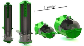
FRIB uses superconducting RF cavities as the main accelerating component. The linac segment contains 4 types of superconducting RF cavities, namely $\beta=0.041$ quarter-wave resonator (QWR), $\beta=0.085$ QWR, $\beta=0.29$ half-wave resonator (HWR) and $\beta=0.53$ HWR, which is shown in Fig. 1 Facco et al. (2012). The physics models for superconducting RF cavities are discussed in this section.

Figure 1: Scheme plot of 4 kinds of superconducting RF cavities used in linac segment, namely left 1: 0.041 QWR, left 2: 0.085 QWR, left 3: 0.29 HWR, left 4: 0.53 HWR.

II.1.1 Longitudinal Model

For a linac, keeping track of the kinetic energy and phase evolution of the reference synchronous particle is important. To ensure precision, the field map integration shown in Eq. 1

$$\left\{\begin{array}[]{l}W(z)=W_{s}+\int_{s}^{z}qE_{z}(z)cos\phi(z)dz\\ \phi(z)=\phi_{s}+\int_{s}^{z}\frac{2\pi}{\beta(z)\lambda}dz\\ \beta(z)=\sqrt{1-\frac{1}{\gamma(z)^{2}}}\\ \gamma(z)=\frac{W(z)}{m_{0}c^{2}}\end{array}\right.$$ (1)

is used. $z$ stands for the longitudinal position. Subscript $s$ stands for start point. $W$ is total energy (rest energy plus kinetic energy). $q$ is charge state. $E_{z}(z)$ is longitudinal electric field map along $z$. $\phi$ is cavity phase. $\lambda$ is speed of light over cavity frequency. $m_{0}c^{2}$ is rest energy.

The first order longitudinal phase space transverse matrix, which is shown in Eq. 2, is used to track the longitudinal phase and energy spread,

$$\left[\begin{array}[]{c}\Delta\phi_{e}\\ \Delta W_{e}\end{array}\right]=\left[\begin{array}[]{cc}1&0\\ -qV_{0}Tsin\phi-qV_{0}Scos\phi&1\end{array}\right]\left[\begin{array}[]{c}\Delta\phi_{s}\\ \Delta W_{s}\end{array}\right]$$ (2)

, where subscript $s$ stands for start point and subscript $e$ stands for end point. $\Delta\phi$ and $\Delta W$ are RMS phase spread and energy spread. $T$ and $S$ are transit time factors (TTFs) for longitudinal electric field. $\phi$ is the cavtity phase at the longitudinal focusing thin lens.

II.1.2 Transverse Model

As can be seen from Fig. 1, these cavities are non-axisymmetric along the beam line. It is known that non-axisymmetric super-conducting RF cavities produce dipole and quadrupole terms in transverse directions, and can cause beam steering and deformation Facco and Zvyagintsev (2011); Cavenago (1992). A multipole-expansion based scheme is implemented in FLAME.

Field Multipole Expansion: Multipole expansion is the traditional method of analyzing multipole components in an electromagnetic field He et al. (2012); Olave et al. (2012); De Silva and Delayen (2013). In the 3-D cylindrical coordinate system the zeroth order of $\phi$ represents the focusing term, the first order represents the dipole or the steering term and the second order represents the quadrupole term. After sampling at a certain z, we get a 2-D vector field in the polar coordinate, then we can transfer the 2-D vector field into two 2-D scalar fields by projection. For each scalar field, we expand the $\rho$ direction into the Taylor series and $\phi$ direction into the Fourier series.The coefficient is proportional to the strength of the certain field mode. The process can be expressed as Eq. 3,

$$F_{\rho,nm}(\rho,\theta)=F_{max}\left[\begin{array}[]{c}1\\ \rho\\ \rho^{2}\\ \rho^{3}\\ ...\\ \rho^{n}\end{array}\right]^{T}\left[\begin{array}[]{ccccc}a_{00}-ib_{00}&a_{01}-ib_{01}&a_{02}-ib_{02}&...&a_{0m}-ib_{0m}\\ a_{10}-ib_{10}&a_{11}-ib_{11}&a_{12}-ib_{12}&...&a_{1m}-ib_{1m}\\ a_{20}-ib_{20}&a_{21}-ib_{21}&a_{22}-ib_{22}&...&a_{2m}-ib_{2m}\\ ...&...&...&...&...\\ a_{n0}-ib_{n0}&a_{n1}-ib_{n1}&a_{n2}-ib_{n2}&...&a_{nm}-ib_{nm}\end{array}\right]\left[\begin{array}[]{c}1\\ e^{i\theta}\\ e^{i2\theta}\\ e^{i3\theta}\\ ...\\ e^{im\theta}\end{array}\right]=F_{max}\sum_{n,m=0}^{\infty}P_{n}A_{nm}\Theta_{m}$$ (3)

. Note that $\rho$ can be usually normalized by $\rho_{m}$, which indicates the cavity aperture, to become an absolute value. $F_{\text{max}}$ is the maximum field value. As a result, $P_{n}$, $A_{nm}$ and $\Theta_{m}$ are all absolute value. Next, we choose FRIB QWR as an example to demonstrate the above method.

E&M fields of FRIB QWRs are simulated using Computer Simulation Technology (CST). Because the CST numerical RF field data is in Cartesian coordinate initially, we first transfer the E&M field into polar coordinate by bilinear interpolation, and then project the 2-D vector field into two 2-D scalar fields. For the particular case of the QWR cavity, because the whole x=0 plane is under the magnetic boundary symmetric condition, we can apply it to simplify the Taylor-Fourier series expansion into Eq. 4,

$$\begin{split}F_{\Omega,ij}=F_{max}\left[\begin{array}[]{c}1\\ \rho\\ \rho^{2}\\ \rho^{3}\\ ...\\ \rho^{n}\end{array}\right]^{T}\left[\begin{array}[]{ccccc}a_{00}&a_{01}&a_{02}&...&a_{0j}\\ a_{10}&a_{11}&a_{12}&...&a_{1j}\\ a_{20}&a_{21}&a_{22}&...&a_{2j}\\ ...&...&...&...&...\\ a_{i0}&a_{i1}&a_{i2}&...&a_{ij}\end{array}\right]\left[\begin{array}[]{c}1\\ sin\theta\\ cos2\theta\\ sin3\theta\\ ...\end{array}\right]\\ F_{\Pi,ij}=F_{max}\left[\begin{array}[]{c}1\\ \rho\\ \rho^{2}\\ \rho^{3}\\ ...\\ \rho^{n}\end{array}\right]^{T}\left[\begin{array}[]{ccccc}a_{00}&a_{01}&a_{02}&...&a_{0j}\\ a_{10}&a_{11}&a_{12}&...&a_{1j}\\ a_{20}&a_{21}&a_{22}&...&a_{2j}\\ ...&...&...&...&...\\ a_{i0}&a_{i1}&a_{i2}&...&a_{ij}\end{array}\right]\left[\begin{array}[]{c}0\\ cos\theta\\ sin2\theta\\ cos3\theta\\ ...\end{array}\right]\end{split}$$ (4)

, where $\Omega$ means $E_{\rho}$ (electric field along radial direction) or $H_{\theta}$ (magnetic field along azimuthal direction), $\Pi$ means $E_{\theta}$ (electric field along azimuthal direction) or $H_{\rho}$ (magnetic field along radial direction). $a_{ij}$ is the multipole coefficient.

To calculate the coefficient of each multipole term, we can make use of the orthogonality of the trigonometric function and integrate with $\sin(k\theta)$ or $\cos(k\theta)$. $k$ is the order number. Then we expand the result into the Taylor series of $\rho$. The coefficient of each order corresponds to the relative strength of the multipole term.

Theoretically, we should expand the field to an infinite order, while in practice, we have to do truncation at a certain order. In principle, we can truncate the expansion to any order as long as all important multipoles have been included. Here, we truncate both the Taylor and the Fourier series to include all linear terms, namely, focusing, dipole and quadrupole terms.

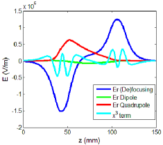
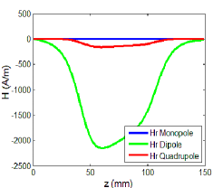
By sampling along the longitudinal direction and calculating multipole coefficients, we can have curves that indicate the multipole field strength versus the longitudinal position. The following Fig. 2 shows the multipole strength curve for the 0.085 QWR electric-magnetic field.

Figure 2: Results of multipole strength curves for radial electric and magnetic fields. (a) The radial electric field multipole strength, defined as $E_{max}$ times multipole term coefficient, v.s. longitudinal coordinate z. Blue curve is (de)focusing term, green curve is dipole term, red curve is quadrupole term, cyan curve is cubic term. (b) The radial magnetic field multipole strength, defined as $H_{max}$ times multipole term coefficient, v.s. longitudinal coordinate $z$. Blue curve is (de)focusing term, green curve is dipole term, and red curve is quadrupole term.

The Multipole Beam Kick Model: After getting out the coefficient matrix from Taylor-Fourier expansion, the multipole beam kick model is used to calculate the beam kick caused by multipole terms. We start from the Lorentz force equation and assume a small acceleration to calculate the change in $y^{\prime}$ in the vertical direction, shown in Eq. 5,

$$\small\begin{split}&\Delta y^{\prime}=\frac{qe\mu_{0}}{\gamma m_{0}}\int_{t_{1}}^{t_{2}}H_{x}(x,y,z,t)dt+\frac{qe}{\gamma m_{0}\beta c}\int_{t_{1}}^{t_{2}}E_{y}(x,y,z,t)dt\\ &=\Delta y^{\prime}_{H,y}+\Delta y^{\prime}_{E,y}\end{split}$$ (5)

, where $q$ is the number of charge, $e$ is the elementary charge amount, $m_{0}$ is the particle static mass, $\mu_{0}$ is the permeability, $c$ is the speed of light. The beam kick can be divided into the magnetic kick and the electric kick. Both kicks can be expressed with a function of $x,y,z$ and $t$. Take the electric kick as an example. If we assume the field is a sinusoidal function about time, then we use $z$ instead of t as an independent variable, and then we get Eq. 6,

$$\Delta y^{\prime}_{E,y}=\frac{qe}{\gamma\beta^{2}m_{0}c^{2}}\int_{z_{1}}^{z_{2}}E_{y}(x,y,z)cos(kz+\phi_{0})dz$$ (6)

, where $\phi_{0}$ is the cavity phase when the particle is at the entrance of the cavity. After transformation and simplification, we can write $E_{y}$ into the following form shown in Eq. 7,

$$E_{y}(x,y,z)=\sum_{i,j=0}^{n}E_{max}(z)a_{ij}(z)t_{ij}(x,y)$$ (7)

. $E_{max}(z)$ is the maximum electric field at the 2-D plane with the longitudinal position $z$. $a_{ij}(z)$ is the multipole coefficient after coordinate transformation. $t_{ij}(x,y)$ is the coordinate transferring factor.

We can substitute it into Eq. 5 and make use of the concept of transit time factors, and get the expression of the vertical beam kick by electric multipole components,

$$\Delta y^{\prime}_{E,y}=\frac{qe}{\gamma\beta^{2}m_{0}c^{2}}\sum_{i,j=0}^{n}t_{ij}V_{ij}(T_{ij}cos\phi-S_{ij}sin\phi)$$ (8)

,where $V_{ij}$ is the voltage of the multipole term $i,j$ defined by integration of multipole term strength $E_{max}A_{ij}(z)$ along longitudinal direction with a unit of Volt. $T_{ij}$ and $S_{ij}$ are the transit time factors of multipole term $i,j$. $\phi$ is the cavity phase at the reference point.

Similarly, we can also get the expression of vertical beam kick by magnetic multipole components,

$$\Delta y^{\prime}_{H,y}=\frac{qe\mu_{0}}{\gamma\beta m_{0}c^{2}}\sum_{i,j=0}^{n}t_{ij}U_{ij}(T_{ij}cos\phi-S_{ij}sin\phi)$$ (9)

. The definition of $U_{ij}$ is similar to $V_{ij}$ except the electric field is changed to the magnetic field, so the unit becomes Ampere.

The entire procedure can be repeated for the calculation of horizontal case.

The Focusing Term: The term with $i=1,j=0$ stands for the beam focusing term. For this case, $E_{max}(z)=E_{max,\rho}(z)$ or the maximum electric field in a 2D plane equals the maximum electric field of the radial projection while the azimuthal projection of the electric field for a focusing term is zero. The coordinate transferring factor $t_{ij}=y/\rho_{m}$. For magnetic field case, the (de)focusing term $H_{max}(z)=H_{max,\theta}(z).t_{ij}=-y/\rho_{m}$. The calculation of the multipole expansion sees very little magnetic (de)focusing term in QWRs and HWRs, so focusing coming from the magnetic (de)focusing term usually can be omitted. Using the model, we can evaluate the focusing or defocusing effect of the cavity.

The Beam Steering Term: The term with $i=0,j=1$ stands for the beam steering term, or the dipole term. For the electric field, $E_{max}(z)=E_{max,\rho}(z)=E_{max,\theta}(z)$, and the coordinate transferring factor $t_{ij}=1$. For the magnetic field, $H_{max}(z)=H_{max,\rho}(z)=H_{max,\theta}(z)$, and $t_{ij}=1$. The calculation of the multipole expansion sees both significant electric and magnetic dipole terms, so we expect that the beam dipole kick can come from both sources.

Using the multipole beam kick model described above, we can calculate the dipole kick and predict beam steering of FRIB QWRs. The results can be benchmarked with particle tracking results, shown in Fig. 3. Both FRIB 0.041 QWR and 0.085 QWR are used. The synchronous phase is fixed at $-\pi/6$, and the accelerating voltage is the design voltage. The green curve indicates the beam steering effect coming from the electric dipole while the cyan curve indicates the beam steering coming from the magnetic dipole. The blue curve is the combination of these two effects and is benchmarked well against the result from 3-D field particle tracking which is plotted in magenta. The difference between the model and 3-D field tracking is plotted in red, note that in the figure the error value is magnified by 10.

Figure 3: Prediction of beam steering by model and tracking vs. $\beta$, synchronous phase $\phi_{s}=-\pi/6$. Blue curve shows the total beam steering calculated by the model, the green and cyan curve each stands for the electric field steering and the magnetic field steering by the model, the magenta curve shows result calculated from tracking, and the red curve shows 10 times the error between the model and tracking; (a) 0.041 QWR; (b) 0.085 QWR.

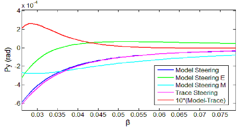
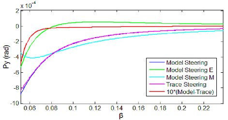
We can see that the precision of the model is high, especially in the high energy region. In the low energy region, particle acceleration in a cavity cannot be neglected so that the error goes up. When the accelerating field of a QWR cavity is fixed, the steering effect would be damping with $\beta$. It is because the higher the energy is, the harder it can be bent by both the electric and magnetic field. Also, damping of the electric field bending effect is faster than that of the magnetic field. So in the high energy region, the dipole steering effect becomes less important and magnetic dipole would be a dominating term. In the low energy region, the dipole steering could become a quite serious problem and some measures should be taken to correct it.

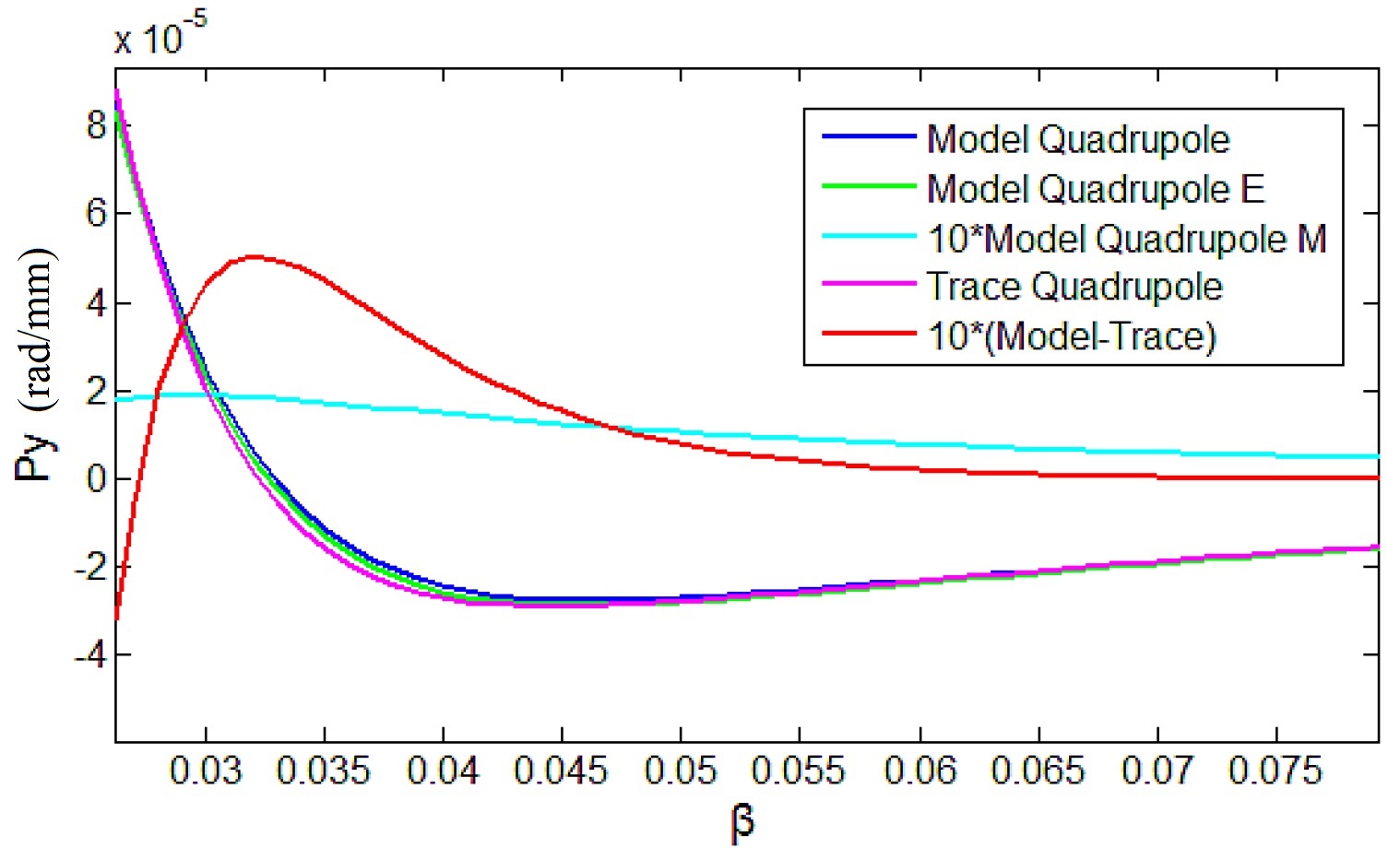
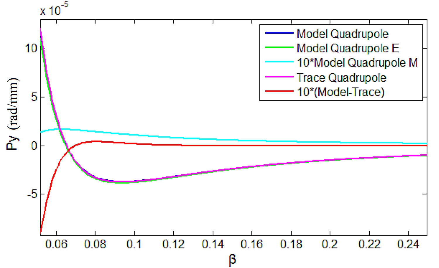
The Quadrupole Term: The term with $i=1,j=2$ stands for the quadrupole term. For the vertical electric field, $E_{max}(z)=E_{max,\rho}(z)=E_{max,\theta}(z)$, the coordinate transferring factor is $t_{ij}=y/\rho_{max}$. For the magnetic field, $H_{max}(z)=H_{max,\rho}(z)=H_{max,\theta}(z)$ , $t_{ij}=y/\rho_{max}$. We can also use the model described above to calculate the quadrupole kick, and then benchmark the calculated quadrupole strength against particle tracking.

Results can be seen in Fig. 4. Both the FRIB 0.041 QWR and 0.085 QWR are used. The synchronous phase is fixed at $-\pi/6$, the accelerating voltage is the design voltage. The green curve stands for the quadrupole kick coming from the electric field and the cyan curve stands for the quadrupole kick coming from the magnetic field (10 times magnified). The blue curve is the total quadrupole kick of the electric and magnetic field contribution added together. We can also see good agreement when comparing the quadrupole kick predicted by the model (blue curve) against the prediction from particle tracking (magenta curve). The error (10 times magnified) is shown in the red curve. According to the model, we can draw the conclusion that the quadrupole kick mainly comes from the electric field and there is nearly no contribution from the magnetic field. The quadrupole effect would also be damping with $\beta$ growing and the effect would be more significant when at low $\beta$.

Figure 4: Prediction of quadrupole strength by the model and tracking vs. $\beta$, the synchronous phase $\phi_{s}=-\pi/6$. The blue curve shows the total quadrupole strength calculated by the model, the green and cyan curve each stands for the electric field quadrupole and 10 times magnified magnetic field quadrupole by the model, the magenta curve shows result calculated from tracking, and the red curve shows 10 times the error between the model and tracking. (a) 0.041 QWR; (b) 0.085 QWR.

The Transverse Thin Lens Model: The transverse drift-kick-drift thin lens model is then developed. The thin lens model includes a series of multipole kicks located at the center of the components, and are separated by a series of drift spaces. For different components, the transfer maps for the transverse phase space are shown as below:

For electric (de)focusing,

$$\begin{split}&\left\{\begin{array}[]{l}x_{2}=x_{1}\\ x_{2}^{\prime}=x_{1}^{\prime}+K_{0}x_{1}\end{array}\right.\left\{\begin{array}[]{l}y_{2}=y_{1}\\ y_{2}^{\prime}=y_{1}^{\prime}+K_{0}y_{1}\end{array}\right.\\ &K_{0}=\frac{qe}{\beta^{2}\gamma m_{0}c^{2}\rho_{m}}V_{E,0}(T_{E,0}cos\phi-S_{E,0}sin\phi)\end{split}$$ (10)

. For the electric dipole,

$$\begin{split}&\left\{\begin{array}[]{l}x_{2}=x_{1}\\ x_{2}^{\prime}=x_{1}^{\prime}\end{array}\right.\left\{\begin{array}[]{l}y_{2}=y_{1}\\ y_{2}^{\prime}=y_{1}^{\prime}+\Delta y^{\prime}\end{array}\right.\\ &\Delta y^{\prime}=\frac{qe}{\beta^{2}\gamma m_{0}c^{2}}V_{E,1}(T_{E,1}cos\phi-S_{E,1}sin\phi)\end{split}$$ (11)

. For the electric quadrupole,

$$\begin{split}&\left\{\begin{array}[]{l}x_{2}=x_{1}\\ x_{2}^{\prime}=x_{1}^{\prime}+K_{q}x_{1}\end{array}\right.\left\{\begin{array}[]{l}y_{2}=y_{1}\\ y_{2}^{\prime}=y_{1}^{\prime}-K_{q}y_{1}\end{array}\right.\\ &K_{q}=\frac{qe}{\beta^{2}\gamma m_{0}c^{2}\rho_{m}}V_{E,2}(T_{E,2}cos\phi-S_{E,2}sin\phi)\end{split}$$ (12)

. For magnetic (de)focusing,

$$\begin{split}&\left\{\begin{array}[]{l}x_{2}=x_{1}\\ x_{2}^{\prime}=x_{1}^{\prime}+K_{0}x_{1}\end{array}\right.\left\{\begin{array}[]{l}y_{2}=y_{1}\\ y_{2}^{\prime}=y_{1}^{\prime}+K_{0}y_{1}\end{array}\right.\\ &K_{0}=\frac{qec\mu_{0}}{\beta\gamma m_{0}c^{2}\rho_{m}}U_{H,0}(T_{H,0}cos\phi-S_{H,0}sin\phi)\end{split}$$ (13)

. For the magnetic dipole,

$$\begin{split}&\left\{\begin{array}[]{l}x_{2}=x_{1}\\ x_{2}^{\prime}=x_{1}^{\prime}\end{array}\right.\left\{\begin{array}[]{l}y_{2}=y_{1}\\ y_{2}^{\prime}=y_{1}^{\prime}+\Delta y^{\prime}\end{array}\right.\\ &\Delta y^{\prime}=\frac{qec\mu_{0}}{\beta\gamma m_{0}c^{2}}U_{H,1}(T_{H,1}cos\phi-S_{H,1}sin\phi)\end{split}$$ (14)

. For the magnetic quadrupole,

$$\begin{split}&\left\{\begin{array}[]{l}x_{2}=x_{1}\\ x_{2}^{\prime}=x_{1}^{\prime}+K_{q}x_{1}\end{array}\right.\left\{\begin{array}[]{l}y_{2}=y_{1}\\ y_{2}^{\prime}=y_{1}^{\prime}-K_{q}y_{1}\end{array}\right.\\ &K_{q}=\frac{qec\mu_{0}}{\beta\gamma m_{0}c^{2}\rho_{m}}U_{H,2}(T_{H,2}cos\phi-S_{H,2}sin\phi)\end{split}$$ (15)

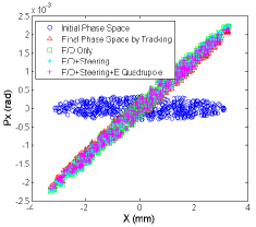
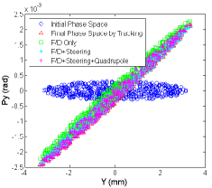
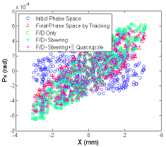
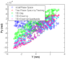
. Subscripts $E,0$, $E,1$ and $E,2$ mean electric (de)focusing, dipole and quadrupole terms. Subscripts $H,0$, $H,1$ and $H,2$ mean magnetic (de)focusing, dipole and quadrupole terms. Then we use the thin lens model for tracking, and the result is benchmarked against 3-D field particle tracking. Both the 0.041 QWR and the 0.085 QWR are tested. The design beta and the design accelerating voltage are used, and the synchronous phase is fixed at $-\pi/6$. The result is shown in Fig. 5. Blue circles represent the initial phase space and red triangles represent the final phase space calculated by 3-D field particle tracking. Green squares show the thin lens model with focusing components only, which tilt both the x and y phase space. Blue stars represent the phase space after adding the steering term. There is no steering effect in the x direction, while in the y direction the steering is about -0.176 mrad for the 0.041 QWR and -0.245 mrad for the 0.085 QWR at design $\beta$. The RMS errors of blue stars for $x,x^{\prime},y,y^{\prime}$ are 0.42%, 5.28%, 0.75%, 2.20% for the 0.041 QWR, and 1.45%, 23.91%, 1.39%, 9.17% for the 0.085 QWR respectively. In the figure, red crosses represent the phase space after adding quadrupole terms. Then the x and y phase spaces become tilted and get closer to the 3-D field particle tracking. The RMS errors of red crosses for $x,x^{\prime},y,y^{\prime}$ become 0.16%, 1.83%, 0.23%, 1.59% for the 0.041 QWR and 0.07%, 4.59%, 0.27%, 2.41% for the 0.085 QWR respectively.

Figure 5: The horizontal phase space and the vertical phase space of a KV distribution beam using tracking and models including different field terms; (a) horizontal phase space, 0.041 QWR; (b) vertical phase space, 0.041 QWR; (c) horizontal phase space, 0.085 QWR; (d) vertical phase space, 0.085 QWR.

II.2 Solenoid

Superconducting solenoids are used as main focusing elements within cryomodules in the FRIB driver linac. A solenoid is modeled by the transport matrix described in Eq. 16  Crandall (1990),

$$M_{\text{sol}}=\left[\begin{array}[]{cccc}C^{2}&\frac{SC}{g}&SC&\frac{S^{2}}{g}\\ -gSC&C^{2}&-gS^{2}&SC\\ -SC&-\frac{S^{2}}{g}&C^{2}&\frac{SC}{g}\\ gS^{2}&-SC&-gSC&C^{2}\end{array}\right]$$ (16)

, where $C=\cos\left(\theta\right)$, $S=\sin\left(\theta\right)$, $g=\frac{B}{2\left(B\rho\right)}$ is the focusing strength , $B$ the magnetic field, $\left(B\rho\right)=\frac{p}{q}$ the particle’s magnetic rigidity, $q$ the charge state, $p$ the momentum, $\theta$ is $gL$. $L$ is the solenoid’s length. For a realistic solenoid, the effective magnetic field strength and length is,

$$\hat{B_{z}}=\frac{\int_{-\infty}^{\infty}B_{z}^{2}(z)}{\int_{-\infty}^{\infty}B_{z}(z)},\hat{L}=\frac{[\int_{-\infty}^{\infty}B_{z}(z)]^{2}}{\int_{-\infty}^{\infty}B_{z}^{2}(z)}$$ (17)

.

II.3 Quadrupole

Room temperature quadrupoles are also used as focusing element outside cryomodules. The 2×2 quadrupole transport matrices (Eq. 18)  Crandall (1990) for a quadrupole with magnetic field gradient $B^{\prime}$ in the focusing and defocusing planes are,

$$\left\{\begin{array}[]{l}F=\left[\begin{array}[]{cc}\cos\left(\sqrt{k}L\right)&\frac{1}{\sqrt{k}}\sin\left(\sqrt{k}L\right)\\ -k\sin\left(\sqrt{k}L\right)&\cos\left(\sqrt{k}L\right)\end{array}\right]\\ D=\left[\begin{array}[]{cc}\cosh\left(\sqrt{k}L\right)&\frac{1}{\sqrt{k}}\sinh\left(\sqrt{k}L\right)\\ k\sinh\left(\sqrt{k}L\right)&\sinh\left(\sqrt{k}L\right)\end{array}\right]\end{array}\right.$$ (18)

, where $k=\left|\frac{B^{\prime}}{\left(B\rho\right)}\right|$ is the focusing strength.

II.4 Dipole

The dipole transport matrix is Eq. 19  Brown et al. (1973) for $\left[x,x^{\prime},y,y^{\prime},l,\delta\right]$,

$$M_{\text{bend}}=\left[\begin{array}[]{cccccc}C&\frac{S}{h_{0}}&0&0&0&\frac{1-C}{h_{0}}\\ -h_{0}S&C&0&0&0&S\\ 0&0&1&L&0&0\\ 0&0&0&1&0&0\\ S&\frac{1-C}{h_{0}}&0&0&1&\alpha_{\mathrm{c}}L\\ 0&0&0&0&0&1\end{array}\right]$$ (19)

, where $C=\cos\left(\alpha\right)$, $S=\sin\left(\alpha\right)$, $h_{0}=\frac{1}{\rho_{0}}$, $\alpha$ the bend angle, $\rho_{0}$ the bend radius, and $\alpha_{\mathrm{c}}$ the momentum compaction,

$$\alpha_{\mathrm{c}}=1-\frac{S}{Lh_{0}}$$ (20)

. For the coordinates used by FLAME $\left[x,x^{\prime},y,y^{\prime},\phi,W\right]$ , the dipole transport matrix is

$$M_{\text{bend}}=\left[\begin{array}[]{cccccc}C&\frac{S}{h_{0}}&0&0&0&\frac{1-C}{h}\frac{1}{\left(pv\right)_{0}}\\ -h_{0}S&C&0&0&0&S\frac{1}{\left(pv\right)_{0}}\\ 0&0&1&L&0&0\\ 0&0&0&1&0&0\\ Sk_{0}&\frac{1-C}{h_{0}}k_{0}&0&0&1&k_{0}\eta_{\mathrm{c}}\frac{L}{\left(pv\right)_{0}}\\ 0&0&0&0&0&1\end{array}\right]$$ (21)

, where $\left(pv\right)_{0}$ is the momentum and velocity for the reference particle, $k_{0}=\frac{2\pi}{\beta_{0}\lambda_{\mathrm{RF}}}$, $\beta_{0}$ and $\gamma_{0}$ are the relativistic factors, and $\eta_{\mathrm{c}}$ is the phase-slip factor,

$$\eta_{\mathrm{c}}=1-\frac{S}{Lh_{0}}-\frac{1}{\gamma_{0}^{2}}$$ (22)

. The transport matrix for edge focusing Eq. 23 is

$$M_{\text{face}}=\left[\begin{array}[]{cccccc}1&0&0&0&0&0\\ h\tan\left(\beta\right)&1&0&0&0&0\\ 0&0&1&0&0&0\\ 0&0&-h\tan(\beta-\psi)&1&0&0\\ 0&0&0&0&1&0\\ 0&0&0&0&0&1\end{array}\right]$$ (23)

, where $\beta$ is the pole face angle, $\psi$ is the correction term resulting from the spatial extent of fringing fields defined as $\psi=K_{1}(\frac{g}{\rho_{0}})(\frac{1+\sin{}^{2}\left(\beta\right)}{\cos\left(\beta\right)})[1-K_{1}K_{2}(\frac{g}{\rho_{0}})\tan\left(\beta\right)]$. $K_{1}$ and $K_{2}$ are the first and second fringe field integral. The full magnet gap width is $g$.

II.5 Electrostatic Element

The front-end section of FRIB uses electrostatic quadrupoles and bends. Beam dynamic models for electrostatic quadrupoles and bends are also included in FLAME. The transport matrix for electrostatic quadrupoles are similar to magnetic quadrupoles. One just need to change the definition of the focusing strength into Eq. 24 Takeda and Billen (2004),

$$k=\frac{2V_{0}}{\left(E\rho\right)R^{2}}$$ (24)

, where $\left(E\rho\right)=$$\frac{pv}{q}$ is the particle’s electric rigidity, $q$ is the charge state, $v$ is the velocity, $V_{0}$ is the voltage of the electrode, and $R$ is the radius.

The transport matrix for a hard edge electrostatic bend is given by Wollnik (2012) and for the coordinates used by FLAME,

$$M_{\text{eb}}=\left[\begin{array}[]{cccccc}C_{x}&\frac{S_{x}}{\sqrt{k_{x}}}&0&0&0&D_{x}N_{W}\frac{1}{W_{0}}\\ -\sqrt{k_{x}}S_{x}&C_{x}&0&0&0&D^{\prime}_{x}N_{W}\frac{1}{W_{0}}\\ 0&0&C_{y}&\frac{S_{y}}{\sqrt{k_{y}}}&0&0\\ 0&0&\sqrt{k_{y}}S_{y}&C_{y}&0&0\\ k_{0}D^{\prime}_{x}N_{t}&k_{0}D_{x}N_{t}&0&0&1&k_{0}\eta_{\mathrm{c}}\frac{L}{W_{0}}\\ 0&0&0&0&0&1\end{array}\right]$$ (25)

, where $C_{x,y}=\cos\left(\sqrt{k_{x,y}}L\right)$, $S_{x,y}=\sin\left(\sqrt{k_{x,y}}L\right)$, $D_{x}=\frac{1-\cos\left(\sqrt{k_{x}}L\right)}{\rho_{0}k_{x}}$, $D^{\prime}_{x}=\frac{\sin\left(\sqrt{k_{x}}L\right)}{\rho_{0}\sqrt{k_{x}}}$, $k_{0}=\frac{2\pi}{\beta_{0}\lambda_{\mathrm{RF}}}$, $N_{W}=\frac{\gamma_{0}^{2}+1}{\gamma_{0}\left(\gamma_{0}+1\right)}$, and $N_{t}=\frac{\gamma_{0}^{2}+1}{\gamma_{0}^{2}}$. $\beta_{0}$, $\gamma_{0}$ are the Lorentz factors. $W_{0}$ is the particle energy. $\lambda_{\mathrm{RF}}$ is the RF wave length. $k_{x}=\frac{1-n_{1}+\gamma_{0}^{2}}{\rho_{0}^{2}}$, $k_{y}=\frac{n_{1}}{\rho_{0}^{2}}$. For a spherical or cylindrical electrostatic bend, $n_{1}=1$ or $n_{1}=0$ respectively. The bend radius is $\rho_{0}$. $K_{0}$ is the kinetic energy of the reference particle, and $\eta_{\mathrm{c}}$ the phase-slip factor

$$\eta_{\mathrm{c}}=\frac{\sqrt{k_{x}}L-S_{x}}{L\rho_{0}^{2}k_{x}^{\nicefrac{{3}}{{2}}}}N_{W}N_{t}-\frac{1}{\gamma_{0}\left(\gamma_{0}+1\right)}$$ (26)

.

The transport matrices for edge focusing are

$$\begin{array}[]{l}M_{\text{entry}}=\left[\begin{array}[]{cccccc}1&0&0&0&0&0\\ -\frac{1}{f^{\prime}_{x}}&\frac{1}{\sqrt{1+\kappa}}&0&0&0&0\\ 0&0&1&0&0&0\\ 0&0&-\frac{1}{f^{\prime}_{y}}&\frac{1}{\sqrt{1+\kappa}}&0&0\\ 0&0&0&0&1&0\\ 0&0&0&0&0&\frac{1}{1+\kappa}\end{array}\right]\\ M_{\text{exit}}=\left[\begin{array}[]{cccccc}1&0&0&0&0&0\\ -\frac{1}{f^{\prime\prime}_{x}}&\sqrt{1+\kappa}&0&0&0&0\\ 0&0&1&0&0&0\\ 0&0&-\frac{1}{f^{\prime\prime}_{y}}&\sqrt{1+\kappa}&0&0\\ 0&0&0&0&1&0\\ 0&0&0&0&0&1+\kappa\end{array}\right]\end{array}$$ (27)

, where $f^{\prime}_{x},f^{\prime}_{y},f^{\prime\prime}_{x},f^{\prime\prime}_{y}$ parameterize the edge focal length; for the details see the Wollnik (2012). The kinetic energy increase factor $\kappa$ is

$$\kappa=\frac{W-W_{0}}{W_{0}}$$ (28)

, which characterizes the effect of particle kinetic energy change due to middle point potential deviation from ground.

The full transport matrix is

$$M_{\text{ebf}}=M_{\text{exit}}M_{\text{eb}}M_{\text{entry}}$$ (29)

.

II.6 Charge Stripper

FRIB is using a charge stripper in folding segment 1 to transfer heavy ions into higher charge states in order to increase the acceleration efficiency Marti et al. (2010). The interaction between the beam and the charge stripper has been simulated with SRIM Ziegler et al. (2010) and then a stripper model has been built by parameterizing the probabilistic distribution within IMPACT-Z Gorelov and Marti (2006). A stripper model is also needed inside FLAME in order to complete beginning to end simulation for FRIB.

There are three main effects which need to be modeled for a stripper: 1) change in charge states, 2) change in the beam energy and 3) blow up in the phase space. The distribution of charge states after the stripper can be calculated using Baron’s formula shown in Eq. 30 Baron and Ricaud (1988); Baron et al. (1993),

$$\left\{\begin{array}[]{l}\frac{\bar{Q}}{Z}=1-exp(-83.275\frac{\beta}{Z^{0}.447})\\ Q_{\text{ave}}=\bar{Q}(1-exp(-12.905+0.2124Z-0.00122Z^{2}))\\ d=\sqrt{\bar{Q}(0.07535+0.19Y-0.2654Y^{2})},Y=\bar{Q}/Z\end{array}\right.$$ (30)

. Here, Gaussian distribution of output charge states is assumed. $Q_{ave}$ is the average output charge state and d is the standard deviation. $\beta$ is the incident beam Lorentz factor, and $Z$ is the number of protons of the incident beam.

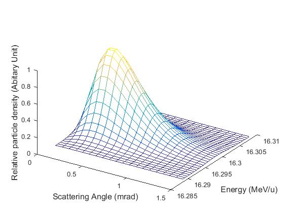
The energy change effect and the phase space blow up effect can be modeled using SRIM. SRIM is a Monte-Carlo code which simulates features of the transport of ions in matter. To build a stripper model for FRIB, we simulated a scenario where an incident 16.623 MeV/u uranium beam with zero emittance is assumed and hit onto a 3 µm carbon stripper. Then, the energy loss and scattering angle are calculated with SRIM. The result can be fitted by Eq.31,

$$f(\theta,E)=\frac{\lambda^{\alpha}}{\Gamma(\alpha)}\theta^{\alpha-1}e^{-\lambda\theta}e^{-\frac{1}{2}[\frac{E-E_{0}}{E_{1}}]^{2}}$$ (31)

. We assume Gamma distribution for the scattering angle and Gaussian distribution for kinetic energy scattering. $\alpha$ and $\lambda$ are parameters related to the shape of the angular distribution, $E_{0}$ is the average beam energy loss after the stripper, and $E_{1}$ is the energy loss distribution width. To simplify the model, we assume $E_{0}$ has no angular dependence. The fitted result can be seen in Fig. 6 below. More cases with different carbon stripper thickness and incident beam energy are simulated, so that we can get fitting parameters over a certain range of stripper thickness and incident beam energy through interpolation.

Figure 6: Energy and scattering angle distribution after an incident 16.623 MeV/u zero emittance uranium beam travels through a 3 µm carbon stripping foil. The three axes are the scattering angle, the output energy, and the relative particle density respectively.

After that, we can model the phase space blow up effect. We assume that the beam does not change in the real space. The overall transverse angular spread can be treated as an extra transverse angular spread, introduced by stripper, adding up to the original angular spread, which can be approximated by Eq. 32,

$$\sigma_{h}=\sqrt{\sigma_{f}^{2}+\sigma_{\Gamma}^{2}}$$ (32)

, where $\sigma_{f}$ is the initial angular spread RMS, and $\sigma_{\Gamma}^{2}=\frac{\alpha}{\lambda^{2}}$ is the RMS of angular Gamma distribution. For the longitudinal energy RMS spread growth, we should also take the foil thickness variation into consideration. Then the output energy RMS spread can be approximated by Eq. 33,

$$\sigma_{h}=\sqrt{\sigma_{f}^{2}+E_{1}^{2}+\sigma_{t}^{2}}$$ (33)

, where $\sigma_{f}$ is the initial energy spread RMS, $E_{1}$ is the energy distribution width calculated above, and $\sigma_{t}$ is the energy spread RMS variation introduced by foil thickness variation. $\sigma_{t}$ can be calculated as $\sigma_{t}=\sigma_{w}t_{foil}E_{0,w}$. $\sigma_{w}$ is the RMS foil variation in percentage, $t_{foil}$ is the foil thickness, and $E_{0,w}$ is the first derivation of $E_{0}$ over the foil thickness. $E_{0,w}$ can be approximated by $\frac{E_{02}-E_{01}}{t_{2}-t_{1}}$, where $E_{02}$ and $E_{01}$ are fit results of $E_{0}$ over two different SRIM simulation with two different stripping foil thickness $t_{2}$ and $t_{1}$.

II.7 Misalignment

Mis-alignments of beam elements are modeled by the Euclidian group for 3D translations

$$\bar{x}\rightarrow\bar{x}-\Delta\bar{x}$$ (34)

and rotations

$$R_{\mathrm{3D}}\left(\bar{\theta}\right)=\left[\begin{array}[]{ccc}m_{11}&m_{12}&m_{13}\\ m_{21}&m_{22}&m_{23}\\ m_{31}&m_{32}&m_{33}\end{array}\right]=R_{z}\left(\theta_{z}\right)R_{y}\left(\theta_{y}\right)R_{x}\left(\theta_{x}\right)$$ (35)

where

$$R_{x}\left(\theta_{x}\right) =\left[\begin{array}[]{ccc}1&0&0\\ 0&\cos\left(\theta_{x}\right)&\sin\left(\theta_{x}\right)\\ 0&-\sin\left(\theta_{x}\right)&\cos\left(\theta_{x}\right)\end{array}\right],$$

$$R_{y}\left(\theta_{y}\right) =\left[\begin{array}[]{ccc}\cos\left(\theta_{y}\right)&0&\sin\left(\theta_{y}\right)\\ 0&1&0\\ -\sin\left(\theta_{y}\right)&0&\cos\left(\theta_{y}\right)\end{array}\right],$$

$$R_{z}\left(\theta_{z}\right) =\left[\begin{array}[]{ccc}\cos\left(\theta_{z}\right)&\sin\left(\theta_{z}\right)&0\\ -\sin\left(\theta_{z}\right)&\cos\left(\theta_{z}\right)&0\\ 0&0&1\end{array}\right]$$

and

$$m_{11} =\cos\left(-\theta_{y}\right)\cos\left(\theta_{z}\right),$$

$$m_{12} =\sin\left(\theta_{x}\right)\sin\left(-\theta_{y}\right)\cos\left(\theta_{z}\right)+\cos\left(\theta_{x}\right)\sin\left(\theta_{z}\right),$$

$$m_{13} =-\cos\left(\theta_{x}\right)\sin\left(-\theta_{y}\right)\cos\left(\theta_{z}\right)+\sin\left(\theta_{x}\right)\sin\left(\theta_{z}\right),$$

$$m_{21} =-\cos\left(-\theta_{y}\right)\sin\left(\theta_{z}\right),$$

$$m_{22} =-\sin\left(\theta_{x}\right)\sin\left(-\theta_{y}\right)\sin\left(\theta_{z}\right)+\cos\left(\theta_{x}\right)\cos\left(\theta_{z}\right),$$

$$m_{23} =\cos\left(\theta_{x}\right)\sin\left(-\theta_{y}\right)\sin\left(\theta_{z}\right)+\sin\left(\theta_{x}\right)\cos\left(\theta_{z}\right),$$

$$m_{31} =\sin\left(-\theta_{y}\right),$$

$$m_{32} =-\sin\left(\theta_{x}\right)\cos\left(-\theta_{y}\right),$$

$$m_{33} =\cos\left(\theta_{x}\right)\cos\left(-\theta_{y}\right)$$

, with Cartesian rotation angles: $\bar{\theta}\equiv\left[\mathrm{tilt,\mathrm{yaw},\mathrm{roll}}\right]$.

The matrix for 6D phase-space translations is

$$T_{\mathrm{ps}}\left(\Delta\bar{x}\right)=\left[\begin{array}[]{ccccccc}1&0&0&0&0&0&-\Delta x\\ 0&1&0&0&0&0&0\\ 0&0&1&0&0&0&-\Delta y\\ 0&0&0&1&0&0&0\\ 0&0&0&0&1&0&-k_{0}\Delta z\\ 0&0&0&0&0&1&0\\ 0&0&0&0&0&0&1\end{array}\right]$$ (36)

and for rotations,

$$R_{\mathrm{ps}}\left(\bar{\theta}\right)=\left[\begin{array}[]{ccccccc}m_{11}&0&m_{12}&0&m_{13}&0&0\\ 0&m_{11}&0&m_{12}&0&m_{13}&0\\ m_{21}&0&m_{22}&0&m_{23}&0&0\\ 0&m_{21}&0&m_{22}&0&m_{23}&0\\ m_{31}&0&m_{32}&0&m_{33}&0&0\\ 0&m_{31}&0&m_{32}&0&m_{33}&0\\ 0&0&0&0&0&0&1\end{array}\right]$$ (37)

. The new transport matrix is

$$M\rightarrow T_{\mathrm{ps}}^{-1}\left(\nicefrac{{L}}{{2}}\right)T_{\mathrm{ps}}^{-1}\left(\Delta\bar{x}\right)R_{\mathrm{ps}}^{-1}\left(\bar{\theta}\right)M$$

$$\times R_{\mathrm{ps}}\left(\bar{\theta}\right)T_{\mathrm{ps}}\left(\Delta\bar{x}\right)T_{\mathrm{ps}}\left(\nicefrac{{L}}{{2}}\right)$$ (38)

$$= \left(R_{\mathrm{ps}}\left(\bar{\theta}\right)T_{\mathrm{ps}}\left(\Delta\bar{x}\right)T_{\mathrm{ps}}\left(\nicefrac{{L}}{{2}}\right)\right)^{-1}M$$ (39)

$$\times R_{\mathrm{ps}}\left(\bar{\theta}\right)T_{\mathrm{ps}}\left(\Delta\bar{x}\right)T_{\mathrm{ps}}\left(\nicefrac{{L}}{{2}}\right)$$ (40)

where $T_{\mathrm{ps}}\left(\nicefrac{{L}}{{2}}\right)$ is a translation to the element center.

II.8 Multi-Charge-State Acceleration

FRIB is accelerating multiple charge states simultaneously in order to enhance the beam current. Accelerations of multiple charge states can be modeled by FLAME via a divide-and-conquer scheme. A three-step scheme is proposed:

Step 1 – Machine initialization by reference charge state: An ideal particle with a central charge state is used to initialize the whole machine, mainly the cavity phase. The result is then recorded as the global beam reference.

Step 2 – Multi-charge-state beam reference orbit initialization: Single particle tracking is used for a reference particle for each charge state beam center and the result is recorded as the local beam reference for each charge state.

Step 3 – Envelope tracking for each charge state: The beam envelope is then tracked using a transport matrix, which is adjusted according to different charge states and reference orbits.

Sometimes the information for the beam center and the beam RMS envelope of the whole beam are required. Then the beam recombination scheme is needed to provide this information. The total beam center can be calculated as Eq. 41,

$$\bar{x}=\frac{\sum_{i}N_{i}\bar{x}_{i}}{N}$$ (41)

, where $\bar{x}$ is the beam center of the whole beam and $\bar{x}_{i}$ is the beam center for each charge state beam. $N$ is the total number of particles and $N_{i}$ is the number of particles for a certain charge state. The total beam RMS can be calculated as Eq. 42,

$$\sigma=\sqrt{\frac{\sum_{i}N_{i}(\sigma_{i}^{2}+\bar{x}_{i}^{2})}{N}}$$ (42)

, where $\sigma$ is the whole beam RMS envelope size, and $\sigma_{i}$ is the RMS beam envelope size for each charge state. The method and the benchmark have been thoroughly discussed in He et al. (2014).

III Software Design of FLAME

The idea of building a light-weighted online model which can handle FRIB special physics challenges dates back to 2012 He et al. (2012). The first working version aiming at testing the physics modeling concept was written in Matlab. Then, the second version of the online model prototype aiming at initial concept verification of online model support for beam commissioning and physics application started its development at the end of 2014 Shen et al. (2015). The second prototype was called Thin Lens Model (TLM)  Shen and He (2015), and was written in Java, with a python interface linking to the physics application prototyping environment with Jpype Jpy . After concept verification of TLM, we started development of FLAME at the end of 2015, which is written in C++ with control room quality. In this section, the software design strategy of FLAME is described.

FLAME contains a C++ core for efficient numerical calculation and a Python wrapper for convenient work flow control. The core concepts of the simulation engine are the Machine, Element, State, and Config. A Config is a container for key/value pairs. This is the interface through which Elements are specialized. The lattice file parser populates a Config, which may then be used to construct a Machine. A Machine represents an ordered list of Elements (Fig. 8)  Davidsaver (2016).

Figure 7: Elements in a Machine

Figure 8: Propagation of State through a list of Elements

A State represents “the beam”, a particle or bunch of particles which pass from Element to Element through a Machine. It keeps track of important beam parameters such as the charge state, the accumulated phase, the kinetic energy, the beam orbit vector and the beam envelope matrix. The operation of the simulation is for an Element to transform a State. This new (output) state is then passed as an input to the next element (Fig. 8).

FLAME uses a free style input lattice file which contains one or more variable definitions, element definitions and beam line definitions. Variables, for example – charge states, initial kinetic energy and initial beam parameters – can be defined as

$$<var\_name>=<value>;$$

, where <value> can be a string, a scalar, vector floating point values or expressions of these types. An element definition takes the form

$$<instance>:<element\_type>,<key>=<value>,...;$$

, supported element type by now including: “drift”, “marker”, “sbend” (for the sector bend), “quadrupole”, “solenoid”, “rfcavity” (for the RF cavity), “stripper”, “edipole” (for the electrostatic dipole) and “equad” (for the electrostatic quadrupole). A beam line definition is constructed from zero or more elements, or beam line names:

$$<instance>:LINE=(<element>,...);$$

After that, a “USE” statement may be given to select which beam line is expanded and used.

$$USE:<instance>;$$

FLAME also has a high level python wrapper for flexible and easy control of FLAME work flow. FLAME python interface allows “on-the-fly” read and write access of the beam and lattice parameter without reloading most data which is already in the memory. And the python interface also makes many online beam tuning tasks, such as, running arbitrary segments of lattice, lattice parameter optimization and development of a virtual accelerator, which is convenient and efficient for developers. FLAME also has a matrix caching capability. If FLAME infers no change of a transfer matrix between two runs, it’ll reuse the cached matrix instead of recalculating it, which would also contribute to speeding up the calculation process.

IV Precision and Speed Benchmark of FLAME

In this section, the calculation precision and calculation speed are benchmarked with FRIB design codes.

In our case, the lattice design codes, which are DIMAD Servranckx and Brown (1984) for the front-end segment and IMPACT-Z for the main linac segment, are used to verify the simulation precision. The calculation speed of FLAME is then discussed and benchmarked with IMPACT-Z. Note that because the length of the front-end segment is short, there is no issue for calculation speed no matter which code we choose, so we only focus on the linac segment which is designed using IMPACT-Z when discussing speed benchmark.

IV.1 Precision

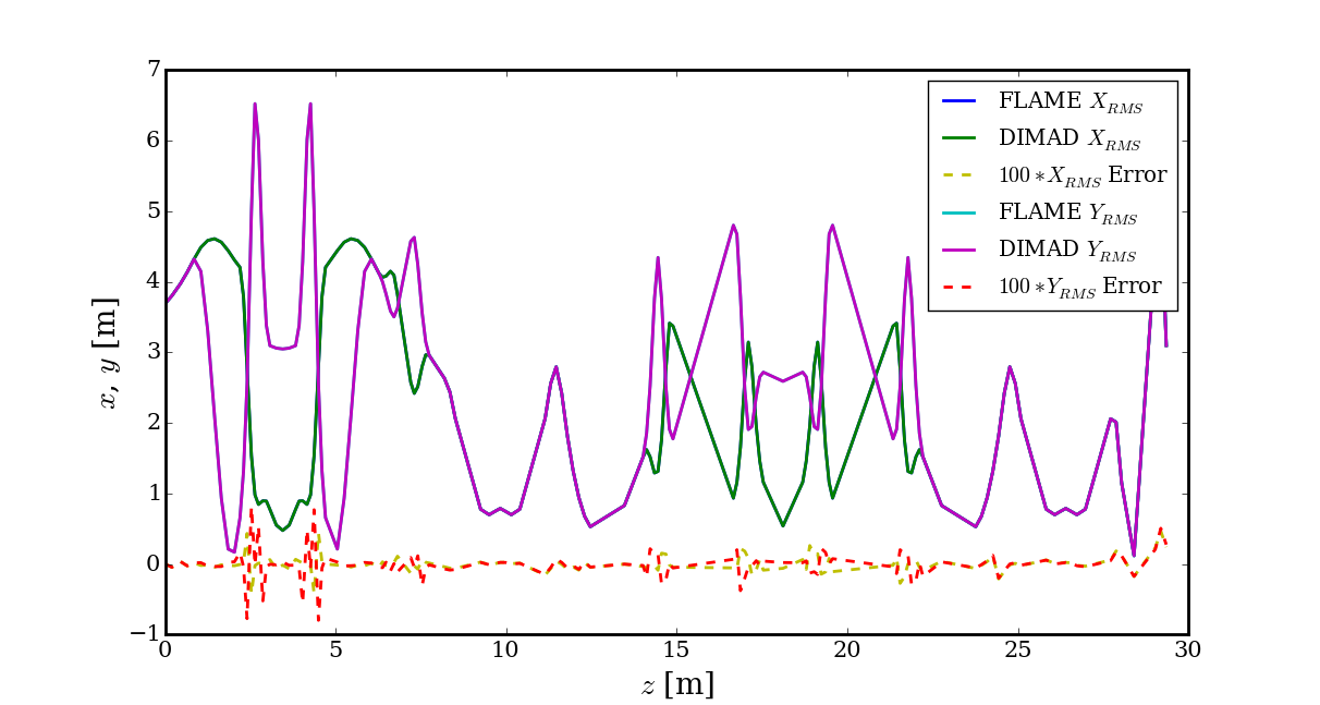
For the front-end segment, the results are benchmarked against DIMAD code. The results for both horizontal and vertical beta-functions are shown in Fig. 9. The RMS error is $1.18\times 10^{-3}$ m for the horizontal beta-function and $1.97\times 10^{-3}$ m for the vertical beta-function. Because the FRIB front-end segment is manipulating coasting beam before the radio-frequency quadrupole, calculation of the longitudinal beam profile is not needed.

Figure 9: The benchmark result between FLAME and DIMAD for the transverse beta-function of front-end segment; blue: FLAME horizontal case; green: DIMAD horizontal case; dashed yellow: 100 times magnified difference between FLAME and DIMAD for horizontal beta-function; cyan: FLAME vertical case; magenta: DIMAD vertical case; dashed red: 100 times magnified error between FLAME and IMPACT-Z for vertical beta-function.

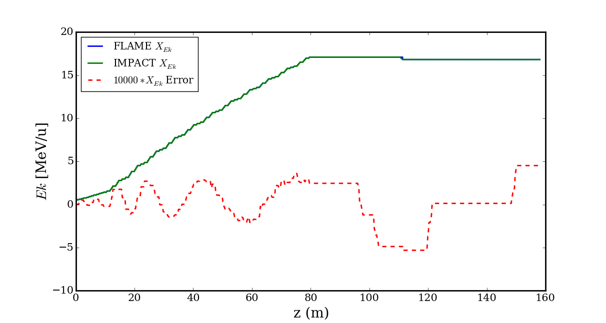
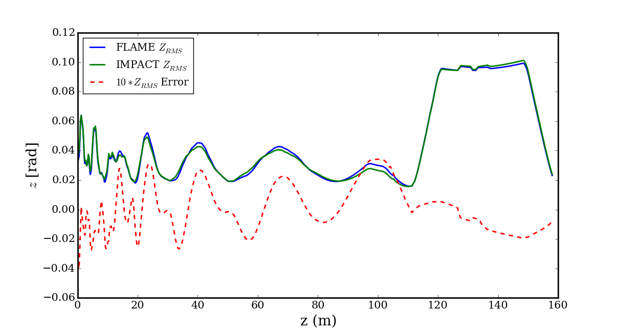
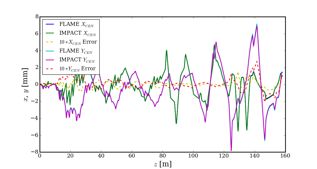
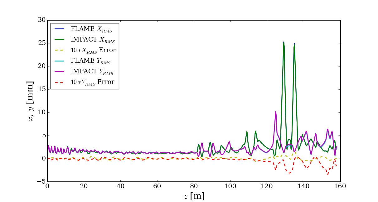
For the main linac, the result needs to be benchmarked in both transverse and longitudinal directions against IMPACT-Z code. The linac segment 1 (LS1) plus folding segment 1 (FS1) of FRIB lattice are used. Uranium 33+ and 34+ before the charge stripper and 76+ to 80+ after the charge stripper are accelerated, and the beam center and the beam envelope after multi-charge-state recombination are benchmarked. The 3D field tracking method is used to handle RF cavities in IMPACT-Z. Fig. 10 shows the benchmark result for the kinetic energy, $2.54\times 10^{-4}$ MeV/u RMS error can be achieved. Fig. 10 shows the benchmark result for the longitudinal RMS size. The RMS error is $1.55\times 10^{-3}$ rad. Fig. 10 shows the benchmark result for the beam orbit with cavity dipole components considered. The RMS error is 0.107 mm for the horizontal direction and 0.128 mm for the vertical direction. Fig. 10 shows the benchmark result for the transverse beam RMS size with cavity quadrupole components considered. The RMS error is 0.091 mm for the horizontal direction and 0.075 mm for the vertical direction.

Figure 10: Benchmark result between FLAME and IMPACT-Z for LS1+FS1. (a) The benchmark result for the kinetic energy; blue: FLAME result, green: IMPACT-Z result; dashed red: 10000 times magnified difference. (b) The benchmark result for the longitudinal RMS size; blue: FLAME result; green: IMPACT-Z result, dashed red: 10 times magnified difference. (c) The benchmark result for the central beam orbit; blue: FLAME horizontal case; green: IMPACT-Z horizontal case; dashed yellow: 10 times magnified difference between FLAME and IMPACT-Z for the horizontal beam orbit; cyan : FLAME vertical case; magenta: IMPACT-Z vertical case; dashed red: 10 times magnified difference between FLAME and IMPACT-Z for the vertical beam orbit. (d) The benchmark result for transverse beam RMS size; blue: FLAME horizontal case; green: IMPACT-Z horizontal case; dashed yellow: 10 times magnified difference between FLAME and IMPACT-Z for the horizontal beam size; cyan: FLAME vertical case; magenta: IMPACT-Z vertical case; dashed red: 10 times magnified error between FLAME and IMPACT-Z for the vertical beam size.

IV.2 Speed

One important design goal for an online model is to ensure fast speed while keeping reasonably high precision. Table 1 shows FLAME running time under various circumstances. A personal laptop with Intel(R) Core(TM) i7-6820HQ CPU @ 2.70 GHz (4 cores 8 threads) is used. FLAME is able to retain all lattice and cavity data information inside the memory, which is easy to edit and reuse. Therefore the initialization time is excluded from the total running time. From column 1 and column 2, we can see that, both C++ API and Python API of FLAME is able to finish calculation within several tens of milli-seconds. And matrix caching is an efficient way of boosting speed of FLAME between two runs where element matrices do not change.

Because IMPACT-Z is a particle tracking code aiming at off-line accelerator design, simply running it will not give satisfactory speed. For example, if we use 20K particles, 3D field tracking based cavity model with integration step 60 to simulate LS1+FS1, the total time it takes is 27 s. However, comparing this time with FLAME does not make sense because this time is not the pure calculation time, and one can always decrease the number of particles and integration steps to increase the speed at the expense of precision. To make a fair comparison between IMPACT-Z and FLAME, we take both the speed and precision into consideration, and make the following assumptions to IMPACT-Z: further improvement to IMPACT-Z can be easily made so that (1) IMPACT-Z can keep the large 3D E&M file in the memory for reuse, so the 3D file loading time (around 12s) can be subtracted from the total time; (2) IMPACT-Z will no longer output the data onto the disk and the file I/O time can be subtracted from the total time; (3) IMPACT-Z will reuse the lattice file which is kept in the memory, so the initialization time can be subtracted from the total time. For FLAME, similar assumptions have already been realized, so no extra assumptions are needed.

Table 1: Running time of FLAME under various circumstances

Performance Benchmark	C++ API [msec]	Python API [msec]	Matrix Cached Run [msec]
1 charge state for LS1	16.0	17.7	6.4
2 charge states for LS1	26.3	28.3	6.5
1 to 5 charge states for LS1+FS1	25.4	28.2	8.0
2 to 5 charge states for LS1+FS1	36.0	39.2	8.2

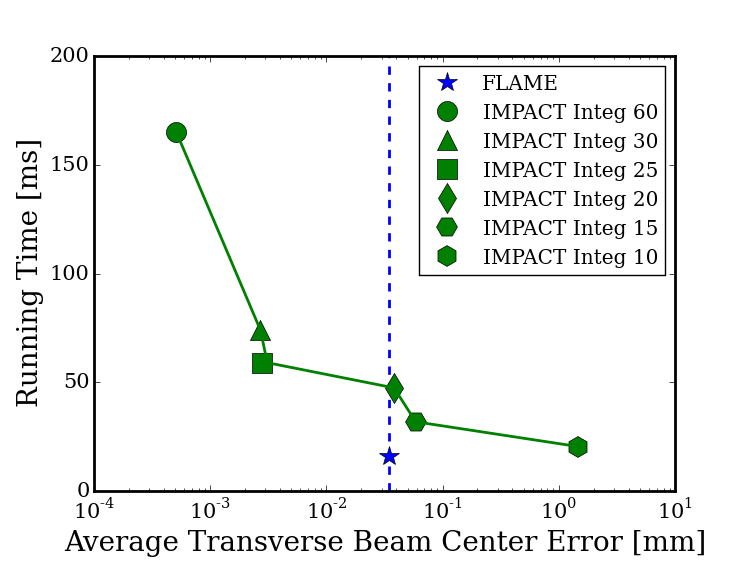
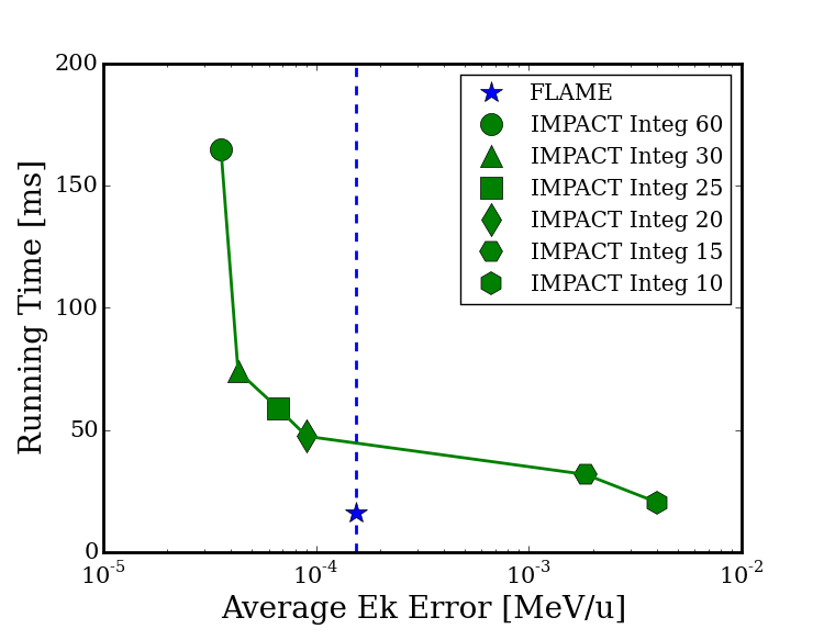
Beam Orbit and Energy: IMPACT-Z can use a single particle to calculate the beam orbit and the reference energy. The integration step of all elements except the RF cavities are set to 1, and the integration step of the RF cavity is treated as a variable. We set the integration step 1000 as a reference case, where the calculation results already converge. The lattice of LS1 is used. Both FLAME and IMPACT-Z are run on the same laptop computer described above. The calculation precision and speed are then compared with FLAME (Fig. 12). Precision of FLAME is comparable to IMPACT-Z with integration steps 20 while 3 times faster. Note that FLAME already gets the envelope information within this period of time as a bonus.

Figure 11: Comparison of the calculation precision and time consumption of beam orbit and kinetic energy between FLAME and IMPACT-Z for a single particle; blue: FLAME case; green: IMPACT-Z case with various integration steps for RF cavity.

Figure 12: Comparison of the calculation precision and the time consumption of transverse and longitudinal beam RMS between FLAME and IMPACT-Z; blue: FLAME case; red: IMPACT-Z case with various particle number, 1 core case; green: IMPACT-Z case with various particle number, 4 cores case.

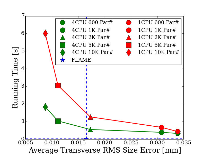
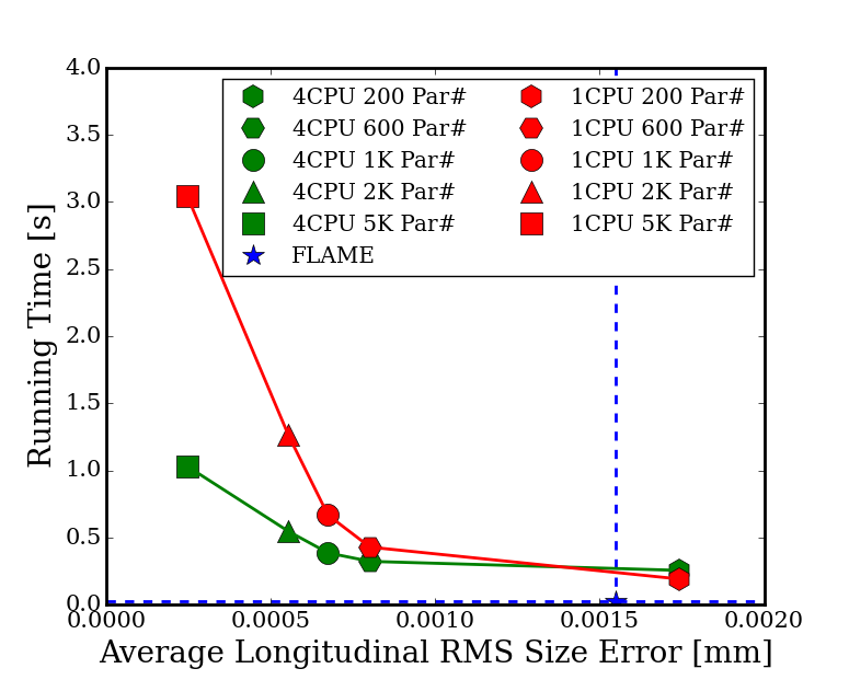
Beam Envelope: The precision of the envelope calculation of IMPACT-Z depends on particle numbers. In this study, the particle number is treated as a variable. We set particle number 100K as a reference case where results already converge. The integration step of all elements except RF cavities is set to 1 and the integration step of RF cavity is set to 30. Lattice of LS1 with 2 charge states is used. Because IMPACT-Z supports message passing interface (MPI) parallelization, we also tested single core and 4 cores cases. The calculation result and speed are then compared with FLAME (Fig. 12). According to the result, the precision of FLAME is comparable to IMPACT-Z with 2K particles for the transverse directions while 48 times faster than 1 core case and 21 times faster than 4 cores case. For longitudinal direction, the precision of FLAME is comparable to IMPACT-Z run with 200 particles and 7 times faster than 1 core case, and 10 times faster than 4 cores case. (MPI overhead may drag down the overall efficiency of IMPACT-Z when the particle number is small)

V CONCLUSION

A new software, FLAME, has been developed for the purpose of FRIB online model service and physics application. FLAME is able to handle the special physics challenges of modeling non-axisymmetric RF cavities and multi-charge state acceleration encountered by FRIB. A multipole expansion based thin-lens cavity model has been thoroughly discussed to handle the dipole and quadrupole terms produced by the non-axisymmetric RF cavities. FLAME contains a C++ core and a python interface for easy access and work flow control. Calculation result benchmark and performance study confirm that FLAME has achieved good balance among precision, speed and convenience, and can be a strong tool in support of FRIB beam commissioning tasks.