Mitigating the Impact of the DESI Fiber Assignment on Galaxy Clustering

Abstract

We present a simple strategy to mitigate the impact of an incomplete spectroscopic redshift galaxy sample as a result of fiber assignment and survey tiling. The method has been designed for the Dark Energy Spectroscopic Instrument (DESI) galaxy survey but may have applications beyond this.

We propose a modification to the usual correlation function that nulls the almost purely angular modes affected by survey incompleteness due to fiber assignment. Predictions of this modified statistic can be calculated given a model of the two point correlation function. The new statistic can be computed with a slight modification to the data catalogues input to the standard correlation function code and does not incur any additional computational time.

Finally we show that the spherically averaged baryon acoustic oscillation signal is not biased by the new statistic.

1 Introduction

Accurate galaxy redshift measurements are obtained from fiber-fed galaxy spectroscopic surveys by observing the positions of recognised features in each galaxy’s spectrum. There have been many such surveys in the past 16 years [1, 2, 3, 4, 5, 6, 7, 8, 9], and several large spectroscopic redshift surveys are planned for the near future [10, 11, 12]. Spectra are collected via optical fibers fed from the target location on the focal plane of the telescope to a spectrograph. Plates are used to hold fibers in place; these are tiled over the footprint of the survey. Each plate represents one set of observations; fibers are reconfigured between observations by switching plates or mechanically moving the positions of the fibers.

In fiber-fed surveys an upper limit to the spectroscopic sample completeness in high density regions is consequently constrained by the physical size of a fiber and the number of fibers available. Additionally, overlap regions in the tiling geometry influence sample completeness and can alter the measured clustering of the galaxy distribution.

To mitigate these effects one may correct the galaxy density field to account for objects that do not get assigned fibers. For example, the BOSS survey BAO analyses [13, 14], up-weighted nearest (spectroscopically observed) neighbours to missed objects. This method assumes that close pairs in angular separation are associated in redshift.

Alternatively one may directly apply corrections to the two-point statistics of the data. For example [15] measure the ratio of the angular correlation functions of parent target sample to observed sample and apply this directly as a weight to the galaxy-galaxy pairs of the correlation function. This corrects the reduction in amplitude of the small scale clustering due to fiber collisions. A different method is used in [16] where the authors divide the galaxy population into non-collided galaxies that will always be observed, population-one and collided galaxies (where the galaxies are too close to simultaneously be assigned fibers), population-two. In regions where the survey tiles overlap, the galaxies in population-two have a greater chance of being observed than those in regions covered by only one tile. They use the statistics of the observed population-two galaxies in tile overlap regions to correct the statistics of the population-two galaxies in areas with lower completeness. They combine the weighted correlation functions of population-one and observed population-two to correct for the non-observed set.

The algorithm we propose in this paper is a modification to the usual correlation function rather than an attempt to recover the lost data. It has been designed specifically for the DESI survey to correct for the effects of tiling and fiber assignment.

In section 2 we give an overview of the DESI survey, the fiber assignment algorithm and the mocks we use for our analysis. In section 3 we propose a modification to the usual correlation function that reduces the effects of fiber assignment and show the modification can be predicted given a model of the two point correlation function. We present the results of the statistic computed with the modified mock data catalogues and fit the BAO peak.

2 The DESI Survey

We start with an overview of the DESI survey, and then discuss the details of the fiber-assignment algorithm.

2.1 An overview of DESI

The Dark Energy Spectroscopic Instrument (DESI) has been designed with the primary goal of measuring the influence of dark energy on the expansion rate of the Universe via baryon acoustic oscillations (BAO) and determining the growth of structure from redshift-space distortions (RSD) [17, 18]. Additionally the observed large-scale structure map will provide a tool to measure the sum of neutrino masses and place constraints on theories of modified gravity and inflation [19].

The ground based instrument will measure the spectroscopic redshifts of objects over five years via ten fiber-fed three-arm spectrographs [20]. It has the capability of measuring 5000 spectra concurrently with fibers located at target positions by robotically-actuated fiber positioners. The instrument will be installed on the 4-m Mayall Telescope at Kitt Peak, Arizona.

The DESI survey will cover 14,000 deg² over which it will measure the spatial distribution of four classes of objects identified from pre-existing and ongoing imaging data [21, 22, 23]. The target classes are luminous red galaxies (LRGs), to be observed up to $z=1.0$, emission line galaxies (ELGs), observed up to $z=1.7$, and quasars (QSO). Quasars will be observed as tracers of the dark matter and the Lyman Alpha absorption features of a high redshift sample of quasars, spanning $2.1<z<3.5$, will be used to probe the intergalactic medium. A further target class, the bright galaxies will utilise the telescope time when the moon is above the horizon and these bright objects will be observed to $z\approx 0.4$ [24].

The precision required to measure the BAO scale, the growth of structure from RSDs and the sum of neutrino masses from the two-point correlation function of observed galaxy pairs means that our measurement must be unbiased. However, the spectroscopic observation method described below, distorts the true two-point statistics of the galaxies.

2.2 Tiling and Fiber Assignment

Figure 1: The left panel shows a ten by ten degree patch of the survey. The blue dots are the simulated ELG observations after pass-1. The tiling pattern is imprinted in the distribution. The right hand panel shows a 1/2 by 1/2 degree patch of the survey. The positions of target galaxies are displayed as black circles. The blue, green, purple, red and yellow points show the simulated observations after pass-1 to 5 respectively. After all five passes the empty circles are the unobserved galaxies.

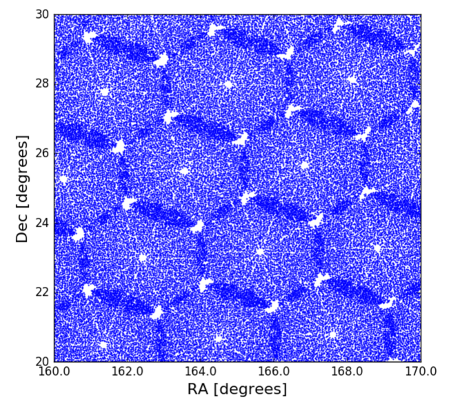
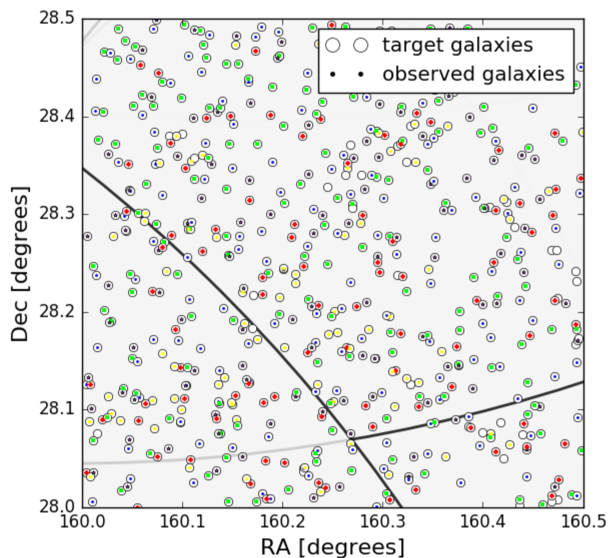
Approximately 2000 pointings (tiles) will cover the survey the footprint (one pass) in a year. The tiles are offset at each pass allowing a total of 10,000 unique tiled observations over five years. Five thousand robotic positioners are located on the focal plane of the telescope which has an instrumented area of about 7.5 sq. deg. Each positioner carries an optical fiber and on completion of an observation, fibers are mechanically moved to a new target position on the tile ready for the next set of observations.

The robotically actuated fiber positioner will be programmed to select targets according to an algorithm that we refer to as the fiber assignment algorithm. Not all DESI targets will be assigned a fiber. The algorithm chooses targets based on their priority, the fiber reach, the number of observations required and the need to avoid collisions between positioners.

The classes of objects to be observed in priority order during dark time are Lyman-alpha QSOs, QSOs, LRGs and ELGs. Consequently after five passes $\sim 80\%$ completeness is expected for the lowest priority ELG sample compared to $\sim 100\%$ for higher priority targets.
The clustering statistics of the ELG sample will be affected by

• Tile overlap; higher completeness in overlap regions.

• Higher priority objects masking targets.

• Fiber size and availability; high density regions get under-sampled due to physical limitations of the fibers.

• Interference from QSO targets which may have correlated overdensities to the ELGs.

The left panel of figure 1 shows a 10 degree by 10 degree patch of the survey. The blue points are the simulated pass 1 observed ELG targets. The tiling pattern is clearly seen in the distribution. The right panel shows a close up of target ELG galaxies within a 1/2 degree by 1/2 degree patch of the survey. The target galaxies are shown as black circles and the different coloured symbols represent which of these galaxies are chosen to be observed by the fiber assignment algorithm at each pass. Empty circles show the missed galaxies. The tiles are in grey outlined in black, although there are no full tiles shown in the figure.

In this work we have used a preliminary version of the DESI fiber assignment scheme [25]. The code takes as input

1. RA and Dec for all targets plus a priority value,

2. RA and Dec for each tile centre,

3. the position of each of the 5000 fibers on the focal plane,

4. a synthetic spectroscopic redshift file to mimic the process of observation,

5. standard star and sky-fiber target files.

The RA and Dec of all targets and each of the 10,000 tile centres are read in; each tile centre has an associated pass number (1-5). The positions of the central body and fiber holder of the fiber positioners are computed to prevent collisions at the time of allocation.

Each fiber on each tile is passed a list of unique target IDs within reach of the fiber; targets are also designated a list of possible fibers.

The code assigns fibers sequentially for each pass by choosing objects with the highest observation priority. If multiple objects share the same priority, objects with the largest number of observations remaining are chosen or if the targets have equal priority and number of observations left, one is chosen at random. The target is marked as observed and the number of remaining observations reflected in subsequent fiber assignment choices. Each tile is assigned 400 sky-fiber and 100 standard star fibers out of 5000. These will be used to determine the sky brightness and calibrate the spectra.

Once fibers have been assigned to targets, two redistribution processes take place. The first identifies targets within range of unused fibers, if a fiber currently assigned to one of those targets can be moved to a new target, this redistribution takes place. This maximises the number of targets that get observed in total. The second process counts the fraction of unused fibers on each tile and adjusts the algorithm so that the fraction is approximately constant over the survey footprint.

Once the fibers have been redistributed, the synthetic real-time observations begin. The synthetic file mimics the observation process and provides the spectroscopic information collected after each pass. The objects assigned to fibers are ‘observed’ and assigned redshifts. If after observation the object is found to be something different from the target class, the observation plan for subsequent passes is updated.

Table 1: Percentage completeness after each pass

pass no.	1	2	3	4	5
ELG completeness (%)	23	44	61	73	81

Table 1 lists the completeness of the ELGs in one of the synthetic catalogues after each pass. The completeness of target samples increases with pass number and at pass-5, spectroscopic redshifts for $\sim 80\%$ of the ELG sample are expected.

In the above observation strategy, the fiber assignment algorithm will have a greater impact on the clustering signal at lower pass numbers where the sample is less complete. Studying the results after just the first pass accentuates the impact of fiber assignment on the two-point correlation function.

For efficiency in the subsequent analysis a simplified version of the code is run on the mock catalogues. This bypasses the redistribution processes. However we find the same conclusions as presented in this paper when running the full code on target files with all types of objects.

2.3 Mocks

We use a set of 25 Quick Particle Mesh (QPM) [26] mock galaxy catalogues to perform our analyses. They are designed specifically for DESI and mimic the survey footprint and radial selection function. These mock catalogues are run though the fiber assignment pipeline; the resulting two-point statistics are shown in section 3.

The QPM mocks are created by generating a low resolution particle mesh using an N-body code. The initial conditions are set using second order Lagrangian Perturbation Theory (2LPT) at $z$=25. At each step the force is computed using Fast Fourier Transforms (FFTs) and a subset of particles (chosen based on local density) are selected as dark matter halos and assigned a halo mass. The mass values are tuned such that the mass function and large-scale bias matches that of higher resolution simulations. Halos are populated with galaxies using the Halo Occupation Distribution (HOD) function of [27]. The ELG HOD is tuned such that the small scale projected correlation function matches that of the blue galaxies with a high star formation rate measured in the DEEP2 survey [28]. The same procedure is carried out for the LRGs such that they have the same power law correlation function as in [29]. The model in [30] is used to create the QSO population.

To compute our two-point statistics, each mock requires a corresponding random catalogue that traces the footprint of the mock but has no spatial correlation between points. To construct the random catalogue, random RA and Dec positions are assigned to particles within the survey footprint. The particles are assigned redshifts so that the random catalogue has the same radial selection function as the average mock selection function at the $\Delta z=0.026$ level. We chose the $\Delta z$ bin to be large enough to contrast with natural fluctuations in the mock galaxy density field along the line of sight. This random catalogue is our parent random catalogue that we use to compute the correlation function of the sample pre-fiber assignment. We run the random catalogue through the fiber assignment algorithm to mimic the variations in completeness in the galaxy sample due to tiling and the physical constraints of the fibers. We call this the fiber-assigned random catalogue and use it to compute the correlation function of the fiber-assigned samples.

3 Fiber Assignment Artifacts

To show the effects of the fiber assignment/tiling and test our method we run 25 QPM survey mock galaxies through the fiber assignment algorithm. We use the publicly available CUTE correlation function code [31] to compute two-point statistics in configuration space. We chose to use the minimum-variance Landy-Szalay estimator [32]

$$\xi\left(r_{\perp},r_{{\mkern 3.0mu\vphantom{\perp}\vrule depth=0.0pt\mkern 2.0mu\vrule depth=0.0pt\mkern 3.0mu}}\right)=\frac{DD\left(r_{\perp},r_{{\mkern 3.0mu\vphantom{\perp}\vrule depth=0.0pt\mkern 2.0mu\vrule depth=0.0pt\mkern 3.0mu}}\right)-2DR\left(r_{\perp},r_{{\mkern 3.0mu\vphantom{\perp}\vrule depth=0.0pt\mkern 2.0mu\vrule depth=0.0pt\mkern 3.0mu}}\right)+RR\left(r_{\perp},r_{{\mkern 3.0mu\vphantom{\perp}\vrule depth=0.0pt\mkern 2.0mu\vrule depth=0.0pt\mkern 3.0mu}}\right)}{RR\left(r_{\perp},r_{{\mkern 3.0mu\vphantom{\perp}\vrule depth=0.0pt\mkern 2.0mu\vrule depth=0.0pt\mkern 3.0mu}}\right)},$$ (3.1)

with 0.25$\,h^{-1}\,{\rm Mpc}$ bin widths for $r_{\perp}$ and $r_{{\mkern 3.0mu\vphantom{\perp}\vrule depth=0.0pt\mkern 2.0mu\vrule depth=0.0pt\mkern 3.0mu}}$ representing the separation distances perpendicular and parallel to the line of sight between two objects. We estimate the one-dimensional multipoles of the data with a Legendre polynomial compression of the two-dimensional correlation function computed with separation $r,\mu$ where

$$r=(r_{\perp}^{2}+r_{{\mkern 3.0mu\vphantom{\perp}\vrule depth=0.0pt\mkern 2.0mu\vrule depth=0.0pt\mkern 3.0mu}}^{2})^{1/2}\phantom{xxxxxx}\mu=\frac{r_{{\mkern 3.0mu\vphantom{\perp}\vrule depth=0.0pt\mkern 2.0mu\vrule depth=0.0pt\mkern 3.0mu}}}{r},$$ (3.2)

so that

$$\xi_{\ell}(r)\approx\frac{2\ell+1}{2}\sum_{j}\Delta\mu_{j}\xi(r,\mu_{j})L_{\ell}(\mu_{j}),$$ (3.3)

where $L_{\ell}$ is the Legendre polynomial of order $\ell$.

Figure 2: Left, the two-dimensional correlation function of the complete sample, centre, the two-dimensional correlation function after 1 pass of the fiber-assignment algorithm computed with fiber-assigned randoms, right, the two-dimensional correlation function after 5 passes of the fiber-assignment algorithm computed with fiber-assigned randoms. The correlation functions of the fiber-assigned data look different to the full sample on scales of $r_{\perp}\lesssim 50\,h^{-1}\,{\rm Mpc}$ where pairs of galaxies with close angular proximity are not observed.

Figure 2 shows the impact of the fiber-assignment and tiling averaged over the 25 mock data catalogues. Note we are using the fiber-assigned randoms as the default random catalogue to compare to fiber-assigned data. When constructing the fiber assigned random catalogue, we ran 4 random catalogues of the same density as the target ELG data through the algorithm and concatenated the output. We used 4 times the number of randoms than data point as this meant running 4 random catalogues (the same size as the mock data) through the fiber-assignment algorithm. To make cosmological measurements we suggest using at least 10 times the number of random points than data points but this was not necessary in our case. Tests using a random catalogue that is uniform in the RA, Dec plane within the footprint of the survey show much larger distortions when compared to the fiber-assigned data. The plots show two dimensional correlation functions $\xi\left(r_{\perp},r_{{\mkern 3.0mu\vphantom{\perp}\vrule depth=0.0pt\mkern 2.0mu\vrule depth=0.0pt\mkern 3.0mu}}\right)$ for the average of the 25 mocks. The plot on the left shows the pre-fiber assignment ‘true’ sample computed with all of the randoms, the centre plot is the sample after 1 pass of the fiber-assignment algorithm the right is the sample after 5 passes of the fiber-assignment algorithm.

The plots show how the combined effect of the fiber assignment algorithm and tiling alter the line of sight distribution of pairs of galaxies with small separations ($r_{\perp}\lesssim 50\,h^{-1}\,{\rm Mpc}$) perpendicular to line of sight compared to the original correlation function on the left.

Figure 3: The top panel of the plot shows the monopole (left), quadrupole (centre) and hexadecapole (right) of the complete sample (black), the pass-1 fiber-assignment data (blue cross) and fiber-assigned pass-5 data (pink dots). The bottom panel shows the difference between the pass-1 and original statistics (blue) and the pass-5 and original statistics (pink). The BAO region is isolated by showing the 80-120 $\,h^{-1}\,{\rm Mpc}$ range. From left to right the panels show the monopole, quadrupole and hexadecapole. The error bars show the standard deviation of the 25 mock catalogues.

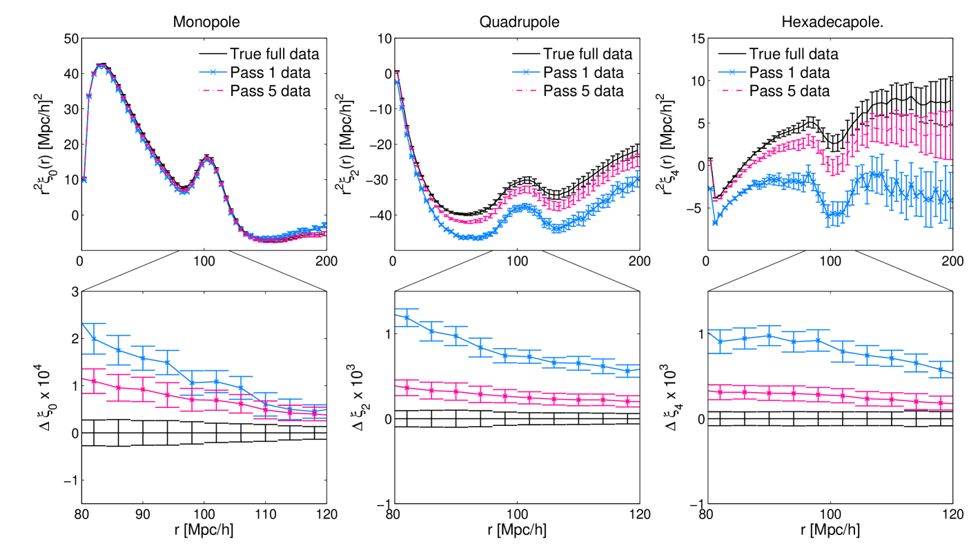
The monopole, quadrupole and hexadecapole of these samples are shown in the top panel of the top plot of figure 3. The monopole (left) of the pass-5 data (pink dots) seems to reproduce the complete sample (black full line) but the pass-1 data (blue crosses) diverge at small and large scales. The lower panel of the top plot zooms in on the BAO scale (80-120 $\,h^{-1}\,{\rm Mpc}$) and shows the differences between the complete sample statistics and the pass-5 and pass-1 data. A similar pattern emerges for the difference in the monopole, quadrupole and hexadecapole showing a change of shape of the function in the BAO region of the fiber-assigned data when compared to the full data set.

3.1 A Modified Algorithm

To repair the structure in the tiled and fiber-assigned data a shuffled random catalogue is created with exactly the same angular clustering as the data but randomly distributed along the line of sight retaining the radial selection function of the survey. This shuffling method was previously used to produce redshifts for the BOSS random catalogue [33]. We replace the random catalogue in the numerator of the correlation function with the shuffled randoms, making our new estimator

$$\tilde{\xi}\left(r_{\perp},r_{{\mkern 3.0mu\vphantom{\perp}\vrule depth=0.0pt\mkern 2.0mu\vrule depth=0.0pt\mkern 3.0mu}}\right)=\frac{DD\left(r_{\perp},r_{{\mkern 3.0mu\vphantom{\perp}\vrule depth=0.0pt\mkern 2.0mu\vrule depth=0.0pt\mkern 3.0mu}}\right)-2DS\left(r_{\perp},r_{{\mkern 3.0mu\vphantom{\perp}\vrule depth=0.0pt\mkern 2.0mu\vrule depth=0.0pt\mkern 3.0mu}}\right)+SS\left(r_{\perp},r_{{\mkern 3.0mu\vphantom{\perp}\vrule depth=0.0pt\mkern 2.0mu\vrule depth=0.0pt\mkern 3.0mu}}\right)}{RR\left(r_{\perp},r_{{\mkern 3.0mu\vphantom{\perp}\vrule depth=0.0pt\mkern 2.0mu\vrule depth=0.0pt\mkern 3.0mu}}\right)},$$ (3.4)

where $S$ is the shuffled random catalogue.

The two-dimensional correlation function of the new statistic is shown before (left) and after fiber assignment (pass-1 centre, pass-5 right) in figure 4. Note that the left hand plot of this figure is different from that in figure 2 as the full sample statistic has been computed with the shuffled random catalogue. The two-dimensional two-point correlation function of the pass-1 and pass-5 data computed with the shuffled random catalogue by eye match those of the whole sample which has the modified feature at small $r_{\perp}$ along the line of sight. To see more clearly the difference between the three data sets we compute the monopole, quadrupole and hexadecapole as before.

Figure 4: Left, the modified two-dimensional correlation function of the complete sample, centre, the modified two-dimensional correlation function of post-fiber assignment pass-1 data, right, the modified two-dimensional correlation function of the post-fiber assignment pass-5 data. All three correlation functions use a shuffled random catalogue and show the same structure.

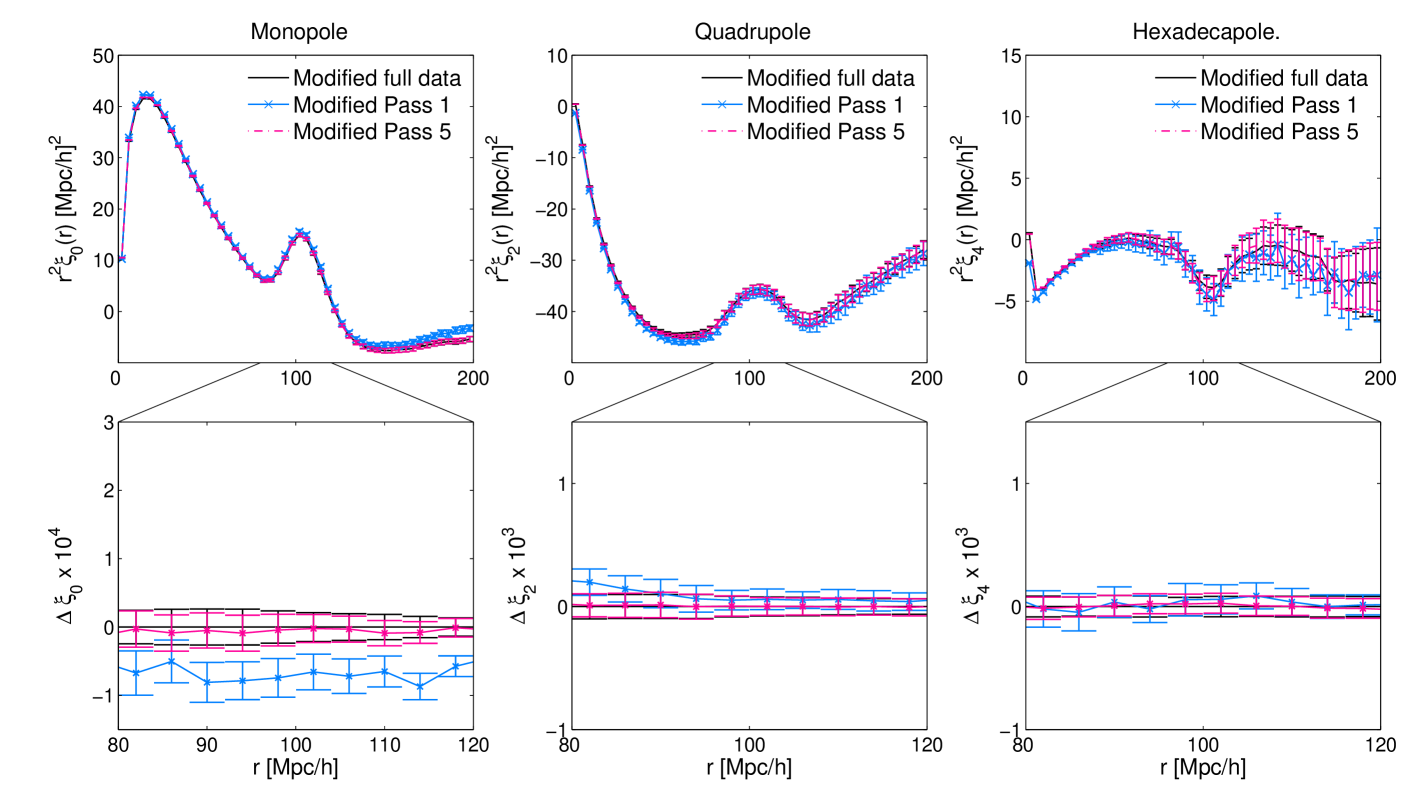
The upper panel of the plot in figure 5 shows the modified monopole, quadrupole and hexadecapole of the complete sample (black full line), pass-1 data (blue crosses) and pass-5 data (pink dots). The statistics of the modified sample at pass-1 and pass-5 seem to recover a noisier version of the complete sample suggesting that the modified statistic approximately removes the effects of the tiling and fiber assignment. The lower panels of the plot show the differences in the data sets. Although the differences show divergence from the original sample at small scales as with the non-modified version, the differences are an order of magnitude smaller and the divergence occurs over a shorter separation range.

Figure 5: The top panel of the plot shows the monopole (left) and quadrupole (centre) and hexadecapole (right) of the modified sample (black), the pass-1 fiber-assignment modified statistic (blue cross) and fiber-assigned pass-5 modified statistic (pink dots).The lower panel of the plot shows the difference between the pass-1 and original statistics (blue) and the pass-5 and original statistics (pink).The BAO region is isolated by showing the 80-120 $\,h^{-1}\,{\rm Mpc}$ range. From left to right the panels show the monopole, quadrupole and hexadecapole. The error bars show the standard deviation of the 25 mock catalogues. Comparing the bottom panel to that of figure 3, it can be seen that the shape difference between the full sample and fiber-assigned samples over the BAO range is much smaller when using the modified correlation functions.

As the systematic effects we are removing are coupled to the angular components of the overdensity, to use the modified statistic we must understand the information being lost. Note that we do not compare the modified correlation function computed using the shuffled randoms to the complete sample (with no fiber assignment) as they are different statistics.

3.2 Understanding the Algorithm

The modified correlation function consists of the galaxy density field ($n$), the shuffled random catalogue ($\tilde{n}$) and the standard random catalogue ($\bar{n}$). We can construct the modified density perturbation, $\tilde{\delta}$ as

$$\tilde{\delta}({\bf r})\equiv\frac{n({\bf r})-\tilde{n}({\bf r})}{\bar{n}({\bf r})},$$ (3.5)

where the shuffled random catalogue contains the angular positions of the galaxies integrated over the survey redshift range. The projected density is then redistributed along the line of sight in a ratio matching the ratio of randoms as a function of redshift,

$$\tilde{n}({\bf r})=\frac{\int n({\bf\gamma},\chi^{\prime})d\chi^{\prime}\int\bar{n}({\bf\gamma}^{\prime},\chi)d{\bf\gamma^{\prime}}}{\int\int\bar{n}({\bf\gamma}^{\prime},\chi^{\prime})d{\bf\gamma}^{\prime}d\chi^{\prime}},$$ (3.6)

where $\gamma$ is the two-dimensional angular coordinate and $\chi$ the line-of-sight coordinate. In terms of $\delta$ the modified overdensity can be written as

$$\tilde{\delta}({\bf r})=\delta({\bf r})-\frac{\int\delta({\bf\gamma},\chi^{\prime})\bar{n}(\chi^{\prime})d{\chi^{\prime}}}{\int\bar{n}(\chi^{\prime})d\chi^{\prime}},$$ (3.7)

where we have assumed that the random catalogue is constant in ${\bf\gamma}$. We note that this method is the configuration space equivalent to nulling the power in the $k_{{\mkern 3.0mu\vphantom{\perp}\vrule depth=0.0pt\mkern 2.0mu\vrule depth=0.0pt\mkern 3.0mu}}=0$ bin in the power spectrum (Pinol et al. in prep). The modified correlation function is the ensemble average of the modified density fluctuations separated by distance $\mathbf{r-r^{\prime}}$ and can be expressed as

$$\begin{split}\langle\tilde{\delta}({\bf r})\tilde{\delta}({\bf r^{\prime}})\rangle&=\left\langle\delta({\bf r})\delta({\bf r^{\prime}})\right\rangle\\ &-2\left\langle\delta({\bf r})\frac{\int\delta({\bf\gamma},\chi^{\prime})\bar{n}(\chi^{\prime})d\chi^{\prime}}{\int\bar{n}(\chi^{\prime})d\chi^{\prime}}\right\rangle\\ &+\left\langle\frac{\int\delta({\bf\gamma},\chi^{\prime})\bar{n}(\chi^{\prime})d\chi^{\prime}}{\int\bar{n}(\chi^{\prime})d\chi^{\prime}}\frac{\int\delta({\bf\gamma}^{\prime},\chi^{\prime\prime})\bar{n}(\chi^{\prime\prime})d\chi^{\prime\prime}}{\int\bar{n}(\chi^{\prime\prime})d\chi^{\prime\prime}}\right\rangle.\end{split}$$ (3.8)

To compute the second term on the right hand side of the above equation we write

$$\left\langle\delta({\bf r})\frac{\int\delta({\bf\gamma},\chi^{\prime})\bar{n}(\chi^{\prime})d\chi^{\prime}}{\int\bar{n}(\chi^{\prime})d\chi^{\prime}}\right\rangle=\frac{\int\xi(\theta,\chi,\chi^{\prime})\bar{n}(\chi^{\prime})d\chi^{\prime}}{\int\bar{n}(\chi^{\prime})d\chi^{\prime}},$$ (3.9)

where $\theta=|\gamma-\gamma^{\prime}|$ and $\xi(\theta,\chi,\chi^{\prime})$ is the correlation function between pairs of galaxies separated along the line-of-sight by distance $\chi-\chi^{\prime}$. We make the assumption that $\xi(\theta,\chi,\chi^{\prime})\bar{n}(\chi^{\prime})d\chi^{\prime}\approx w(\theta)\bar{n}(\chi^{\prime})d\chi^{\prime}$, i.e. the angular correlation function, therefore the second term in equation 3.8 is two times the angular correlation function. Using the Limber approximation [34] we can write out the angular correlation function as

$$w(\theta)\approx\int\bar{n}^{2}(\chi^{\prime})\int\xi(r_{\perp},r_{{\mkern 3.0mu\vphantom{\perp}\vrule depth=0.0pt\mkern 2.0mu\vrule depth=0.0pt\mkern 3.0mu}}^{\prime})dr^{\prime}_{{\mkern 3.0mu\vphantom{\perp}\vrule depth=0.0pt\mkern 2.0mu\vrule depth=0.0pt\mkern 3.0mu}}d\chi^{\prime}\left(\int\bar{n}(\chi^{\prime})d\chi^{\prime}\right)^{-2}.$$ (3.10)

Finally equation 3.8 becomes

$$\begin{split}\langle\tilde{\delta}({\bf r})\tilde{\delta}({\bf r^{\prime}})\rangle&=\left\langle\delta({\bf r})\delta({\bf r^{\prime}})\right\rangle\\ &-2\int\bar{n}^{2}(\chi^{\prime})\int\xi(r_{\perp},r_{{\mkern 3.0mu\vphantom{\perp}\vrule depth=0.0pt\mkern 2.0mu\vrule depth=0.0pt\mkern 3.0mu}}^{\prime})dr^{\prime}_{{\mkern 3.0mu\vphantom{\perp}\vrule depth=0.0pt\mkern 2.0mu\vrule depth=0.0pt\mkern 3.0mu}}d\chi^{\prime}\left(\int\bar{n}(\chi^{\prime})d\chi^{\prime}\right)^{-2}\\ &+\left\langle\frac{\int\delta({\bf\gamma},\chi^{\prime})\bar{n}(\chi^{\prime})d\chi^{\prime}}{\int\bar{n}(\chi^{\prime})d\chi^{\prime}}\frac{\int\delta({\bf\gamma}^{\prime},\chi^{\prime\prime})\bar{n}(\chi^{\prime\prime})d\chi^{\prime\prime}}{\int\bar{n}(\chi^{\prime\prime})d\chi^{\prime\prime}}\right\rangle.\end{split}$$ (3.11)

The last term in the equation becomes negligible when the survey covers a large comoving distance in which case the model of the corrected correlation function can be written as

$$\tilde{\xi}(r_{\perp},r_{{\mkern 3.0mu\vphantom{\perp}\vrule depth=0.0pt\mkern 2.0mu\vrule depth=0.0pt\mkern 3.0mu}})=\xi(r_{\perp},r_{{\mkern 3.0mu\vphantom{\perp}\vrule depth=0.0pt\mkern 2.0mu\vrule depth=0.0pt\mkern 3.0mu}})-2\iint\xi(r_{\perp},r_{{\mkern 3.0mu\vphantom{\perp}\vrule depth=0.0pt\mkern 2.0mu\vrule depth=0.0pt\mkern 3.0mu}}^{\prime})\bar{n}^{2}(\chi)dr_{{\mkern 3.0mu\vphantom{\perp}\vrule depth=0.0pt\mkern 2.0mu\vrule depth=0.0pt\mkern 3.0mu}}^{\prime}d\chi\left(\int\bar{n}(\chi)d\chi\right)^{-2}.$$ (3.12)

The correction becomes smaller as the radial range of the survey increases and as the radial range tends towards zero the full correction becomes equivalent to the original correlation function.

3.3 Modelling the modified correlation function

In this subsection we compare our model (3.12) to the modified correlation function measured in the full modified data set (with shuffled randoms). Figure 6 shows the model, constructed as in equation 3.12 using the $\xi(r_{\perp},r_{{\mkern 3.0mu\vphantom{\perp}\vrule depth=0.0pt\mkern 2.0mu\vrule depth=0.0pt\mkern 3.0mu}})$ of the full (non-fiber-assigned) sample. The average of the model computed from the 25 mocks is shown as a black line and compared to the average modified two-point statistics (blue crosses) of the mock data computed with the shuffled randoms. The monopole and quadrupole by eye are a very good match. The hexadecapole shows a reasonable match but this inconsistencies may be due to the fact we use $\xi\left(r_{\perp},r_{{\mkern 3.0mu\vphantom{\perp}\vrule depth=0.0pt\mkern 2.0mu\vrule depth=0.0pt\mkern 3.0mu}}\right)$ to construct the model and then translate to the $\mu,r$ coordinate system.

Figure 6: The top panel of the plot shows the average monopole (left), quadrupole (centre) and hexadecapole (right) of the 25 mocks for the model in 3.12 (black line), (non-modified) full correlation function (pink dashed line) and the modified two-point statistics (shuffled randoms, blue crosses). The bottom panel shows the differences between them in the 80-120 $\,h^{-1}\,{\rm Mpc}$ region. The error bars are the standard deviation of the mocks. The black line has error bars as the model is constructed from the correlation function of the full sample mocks. There are deviations between the model and the modified data on small scales however these are much smaller in the BAO region shown in the bottom panel. The non-modified correlation function however shows deviations from this line (in the bottom panel) that would not be captured by adjusting the broadband parameters as they change the shape of correlation functions in the BAO region shown.

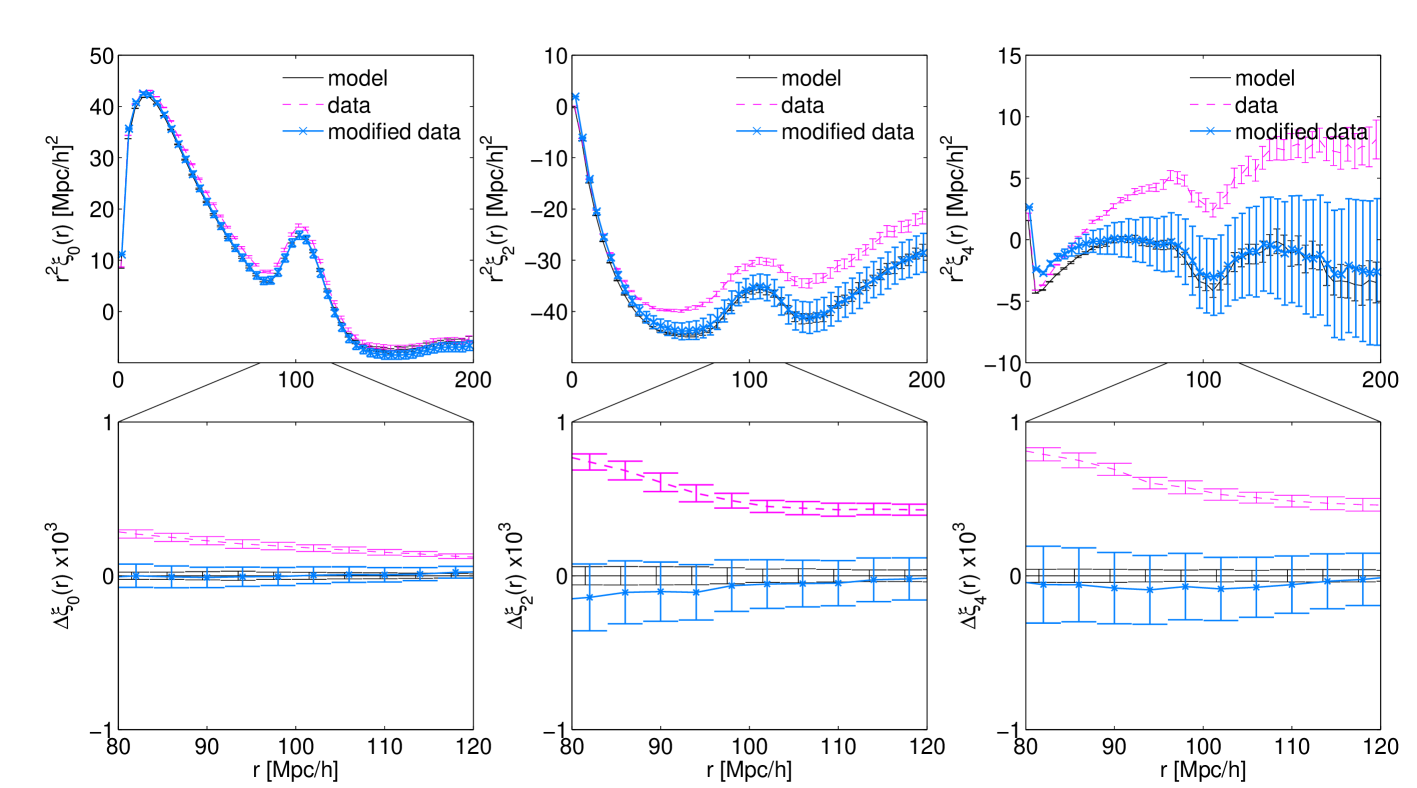
To get a quantitive comparison of the model and the data, we take the $\chi^{2}$ values

$$\chi^{2}(\alpha)=[{\bf d-m(\alpha)}]^{\textrm{T}}C^{-1}[{\bf d-m(\alpha)}],$$ (3.13)

where ${\bf d}$ is the modified correlation function vector of a mock as outlined in equation 3.4 and ${\bf m}$ is the model of the correlation function outlined in equation 3.12 which has been computed from the full data set. As we only have 25 mock catalogues we use the publicly available covariance matrix of the DR11 CMASS BOSS galaxy sample and rescale it so that

$$\textrm{C}=\frac{V_{BOSS}}{V_{DESI}}\textrm{C}_{BOSS}$$ (3.14)

where V${}_{\textrm{BOSS}}$ = 10Gpc³, and V${}_{\textrm{DESI}}$ = 170 Gpc³ are the volumes of the BOSS (CMASS) and DESI survey respectively.

Figure 7: The $\chi^{2}$ values computed for each mock when compared to the model (which is computed from the full data). The mean of the distribution is shown by the vertical line. The $\chi^{2}$ values are higher than expected due to the conversion to the $r,\mu$ coordinate system where $\mu$ bins on small scales are coarsely sampled compared to the large scales.

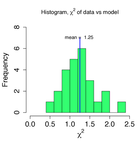
Figure 7 shows histogram $\chi^{2}$ values computed for each mock. The mean $\chi^{2}$ value is close to one. The statistic however also includes the errors introduced when converting the coordinate systems from $r_{\perp},r_{{\mkern 3.0mu\vphantom{\perp}\vrule depth=0.0pt\mkern 2.0mu\vrule depth=0.0pt\mkern 3.0mu}}$ to $r,\mu$ and therefore we expect this to be a very conservative estimate.

To ascertain the usefulness of the model we follow [13, 14] and fit the modified correlation functions of the 25 mock catalogues to the function

$$\textrm{B}^{2}\xi(r\alpha)_{\textrm{model}}+\frac{\textrm{a}_{1}}{r^{2}}+\frac{\textrm{a}_{2}}{r}+\textrm{a}_{3},$$ (3.15)

where a_i, are parameters that marginalise over the broadband shape and the B parameter adjusts the amplitude of the full correlation function. The parameter that we are interested in is $\alpha$ as this encodes any shifts in the BAO feature compared to the original data. We increment $\alpha$ in bins of width $\Delta\alpha=0.001$ in the range $0.95<\alpha<1.05$. The range we have chosen is small as we know the true position of the BAO bump in our data and therefore we are not trying to measure cosmology but rather look for deviations from $\alpha=1$ and the variance of the modified correlation functions compared to the model.

For each $\alpha$ value we compute the best fit values of the 4 parameters and compute the $\chi^{2}$ as in equation 3.13 but where ${\bf d}$ is the modified correlation function vector of a mock as before and ${\bf m}$ is the model of the correlation function with best fit parameters as in equation 3.15 for a given $\alpha$ value.

The mean $\alpha$ values computed from the modified correlation functions is 1.000, and the standard deviation of the mocks compared to the average best fit model is $\sigma_{\alpha}=0.0066$. The mean $\alpha$ from the true correlation function is 1.000 (as expected) and the standard deviation is $\sigma_{\alpha}=0.0067$. We therefore conclude that the modified correlation function is unbiased with respect to recovery of $\alpha$ and the error on this value.

4 Discussion

In this paper we have described an approximation of the tiling and fiber assignment algorithm that will be used in the DESI survey to place fibers on target objects and collect spectroscopic redshifts.

We have shown that the angular clustering coupled with the spectroscopic observation method alters the two-point statistics in early stages of the survey when sample completeness is low. A simple method of mitigating these effects has been presented and tested on mock catalogues. The method uses a modified correlation function that removes small scale angular clustering. The modified correlation functions of the lower completeness data sets that mimic the year 1 and year 5 DESI ELG sample recover the modified statistics of the full sample with an order of magnitude improvement over the non-modified statistic.

We have demonstrated that although information about the small scale angular clustering is lost, the modified correlation function, monopole, quadrupole can be modelled. The lost information is not detrimental to our spherically averaged BAO cosmological analysis although we have not tested the effect of the model on the anisotropic BAO analysis as yet. The study of RSD measurements and the analysis of the anisotropic BAO measurements are deferred to future work. The modified correlation function is only removing information perpendicular to the line of sight where $\mu=0$, thus the RSD signal should not be modified. However the RSD signal is related to the density of the local environment and high density peaks may be flattened using this method.

By nulling the $k_{{\mkern 3.0mu\vphantom{\perp}\vrule depth=0.0pt\mkern 2.0mu\vrule depth=0.0pt\mkern 3.0mu}}=0$ modes, it is possible to mitigate systematic errors associated with imaging data that are restricted to this plane. Again this is worth further investigation.

We have not investigated how the modified catalogues will affect the reconstruction technique [35, 36, 37]. The modified catalogues alter the over-density in an anisotropic way thus will distort the reconstruction displacement vectors. The effects should be investigated before applying reconstruction to the modified catalogues.

This new statistic will allow one to make robust cosmological measurements of the BAO feature from early DESI data if the current observation plan is implemented.

Although the method has been designed specifically for the DESI survey we note that it may be useful in other fiber-fed spectroscopic surveys where the sample completeness is limited in angular resolution due to hardware constraints or the observed sample clustering is affected by the tiling pattern.

References

- [1] D. G. York, J. Adelman, J. E. Anderson, Jr., S. F. Anderson, J. Annis, N. A. Bahcall et al., The Sloan Digital Sky Survey: Technical Summary, AJ 120 (Sept., 2000) 1579–1587, [astro-ph/0006396].
- [2] M. Colless, G. Dalton, S. Maddox, W. Sutherland, P. Norberg, S. Cole et al., The 2dF Galaxy Redshift Survey: spectra and redshifts, MNRAS 328 (Dec., 2001) 1039–1063, [astro-ph/0106498].
- [3] C. Stoughton, R. H. Lupton, M. Bernardi, M. R. Blanton, S. Burles, F. J. Castander et al., Sloan Digital Sky Survey: Early Data Release, AJ 123 (Jan., 2002) 485–548.
- [4] M. Davis, S. M. Faber, J. Newman, A. C. Phillips, R. S. Ellis, C. C. Steidel et al., Science Objectives and Early Results of the DEEP2 Redshift Survey, in Discoveries and Research Prospects from 6- to 10-Meter-Class Telescopes II (P. Guhathakurta, ed.), vol. 4834 of Proc. SPIE, pp. 161–172, Feb., 2003. astro-ph/0209419. DOI.
- [5] M. J. Drinkwater, R. J. Jurek, C. Blake, D. Woods, K. A. Pimbblet, K. Glazebrook et al., The WiggleZ Dark Energy Survey: survey design and first data release, MNRAS 401 (Jan., 2010) 1429–1452, [0911.4246].
- [6] S. P. Driver, D. T. Hill, L. S. Kelvin, A. S. G. Robotham, J. Liske, P. Norberg et al., Galaxy and Mass Assembly (GAMA): survey diagnostics and core data release, MNRAS 413 (May, 2011) 971–995, [1009.0614].
- [7] F. Beutler, C. Blake, M. Colless, D. H. Jones, L. Staveley-Smith, L. Campbell et al., The 6dF Galaxy Survey: baryon acoustic oscillations and the local Hubble constant, MNRAS 416 (Oct., 2011) 3017–3032, [1106.3366].
- [8] K. S. Dawson, D. J. Schlegel, C. P. Ahn, S. F. Anderson, É. Aubourg, S. Bailey et al., The Baryon Oscillation Spectroscopic Survey of SDSS-III, The Astrophysical Journal 145 (Jan., 2013) 10, [1208.0022].
- [9] L. Guzzo, M. Scodeggio, B. Garilli, B. R. Granett, A. Fritz, U. Abbas et al., The VIMOS Public Extragalactic Redshift Survey (VIPERS). An unprecedented view of galaxies and large-scale structure at 0.5 z 1.2, A&A 566 (June, 2014) A108, [1303.2623].
- [10] M. Levi, C. Bebek, T. Beers, R. Blum, R. Cahn, D. Eisenstein et al., The DESI Experiment, a whitepaper for Snowmass 2013, ArXiv e-prints (Aug., 2013) , [1308.0847].
- [11] G. Dalton, S. C. Trager, D. C. Abrams, D. Carter, P. Bonifacio, J. A. L. Aguerri et al., WEAVE: the next generation wide-field spectroscopy facility for the William Herschel Telescope, in Society of Photo-Optical Instrumentation Engineers (SPIE) Conference Series, vol. 8446 of Society of Photo-Optical Instrumentation Engineers (SPIE) Conference Series, Sept., 2012. DOI.
- [12] R. S. de Jong, O. Bellido-Tirado, C. Chiappini, É. Depagne, R. Haynes, D. Johl et al., 4MOST: 4-metre multi-object spectroscopic telescope, in Society of Photo-Optical Instrumentation Engineers (SPIE) Conference Series, vol. 8446 of Society of Photo-Optical Instrumentation Engineers (SPIE) Conference Series, Sept., 2012. 1206.6885. DOI.
- [13] L. Anderson, E. Aubourg, S. Bailey, F. Beutler, A. S. Bolton, J. Brinkmann et al., The clustering of galaxies in the SDSS-III Baryon Oscillation Spectroscopic Survey: measuring DA and H at z = 0.57 from the baryon acoustic peak in the Data Release 9 spectroscopic Galaxy sample, MNRAS 439 (Mar., 2014) 83–101, [1303.4666].
- [14] L. Anderson, É. Aubourg, S. Bailey, F. Beutler, V. Bhardwaj, M. Blanton et al., The clustering of galaxies in the SDSS-III Baryon Oscillation Spectroscopic Survey: baryon acoustic oscillations in the Data Releases 10 and 11 Galaxy samples, MNRAS 441 (June, 2014) 24–62, [1312.4877].
- [15] E. Hawkins, S. Maddox, S. Cole, O. Lahav, D. S. Madgwick, P. Norberg et al., The 2dF Galaxy Redshift Survey: correlation functions, peculiar velocities and the matter density of the Universe, MNRAS 346 (Nov., 2003) 78–96, [astro-ph/0212375].
- [16] H. Guo, I. Zehavi and Z. Zheng, A New Method to Correct for Fiber Collisions in Galaxy Two-point Statistics, ApJ 756 (Sept., 2012) 127, [1111.6598].
- [17] DESI Collaboration, A. Aghamousa, J. Aguilar, S. Ahlen, S. Alam, L. E. Allen et al., The DESI Experiment Part I: Science,Targeting, and Survey Design, ArXiv e-prints (Oct., 2016) , [1611.00036].
- [18] DESI Collaboration, A. Aghamousa, J. Aguilar, S. Ahlen, S. Alam, L. E. Allen et al., The DESI Experiment Part II: Instrument Design, ArXiv e-prints (Oct., 2016) , [1611.00037].
- [19] A. Font-Ribera, P. McDonald, N. Mostek, B. A. Reid, H.-J. Seo and A. Slosar, DESI and other Dark Energy experiments in the era of neutrino mass measurements, JCAP 5 (May, 2014) 023, [1308.4164].
- [20] S. A. Smee, J. E. Gunn, A. Uomoto, N. Roe, D. Schlegel, C. M. Rockosi et al., The Multi-object, Fiber-fed Spectrographs for the Sloan Digital Sky Survey and the Baryon Oscillation Spectroscopic Survey, The Astrophysical Journal 146 (Aug., 2013) 32, [1208.2233].
- [21] B. Flaugher, H. T. Diehl, K. Honscheid, T. M. C. Abbott, O. Alvarez, R. Angstadt et al., The Dark Energy Camera, AJ 150 (Nov., 2015) 150, [1504.02900].
- [22] E. L. Wright, P. R. M. Eisenhardt, A. K. Mainzer, M. E. Ressler, R. M. Cutri, T. Jarrett et al., The Wide-field Infrared Survey Explorer (WISE): Mission Description and Initial On-orbit Performance, AJ 140 (Dec., 2010) 1868–1881, [1008.0031].
- [23] A. Dey, D. Rabinowitz, A. Karcher, C. Bebek, C. Baltay, D. Sprayberry et al., Mosaic3: a red-sensitive upgrade for the prime focus camera at the mayall 4m telescope, 2016. 10.1117/12.2231488.
- [24] R. H. Wechsler and DESI Collaboration, The Dark Energy Spectroscopic Instrument (DESI): Bright-Time Science Program, in American Astronomical Society Meeting Abstracts, vol. 225 of American Astronomical Society Meeting Abstracts, p. 336.06, Jan., 2015.
- [25] R. N. Cahn, S. J. Bailey, K. S. Dawson, J. Forero Romero, D. J. Schlegel, M. White et al., The Dark Energy Spectroscopic Instrument (DESI): Tiling and Fiber Assignment, in American Astronomical Society Meeting Abstracts, vol. 225 of American Astronomical Society Meeting Abstracts, p. 336.10, Jan., 2015.
- [26] M. White, J. L. Tinker and C. K. McBride, Mock galaxy catalogues using the quick particle mesh method, MNRAS 437 (Jan., 2014) 2594–2606, [1309.5532].
- [27] J. L. Tinker, E. S. Sheldon, R. H. Wechsler, M. R. Becker, E. Rozo, Y. Zu et al., Cosmological Constraints from Galaxy Clustering and the Mass-to-number Ratio of Galaxy Clusters, ApJ 745 (Jan., 2012) 16, [1104.1635].
- [28] N. Mostek, A. L. Coil, M. Cooper, M. Davis, J. A. Newman and B. J. Weiner, The DEEP2 Galaxy Redshift Survey: Clustering Dependence on Galaxy Stellar Mass and Star Formation Rate at z ~ 1, ApJ 767 (Apr., 2013) 89, [1210.6694].
- [29] M. White, M. Blanton, A. Bolton, D. Schlegel, J. Tinker, A. Berlind et al., The Clustering of Massive Galaxies at z ~ 0.5 from the First Semester of BOSS Data, ApJ 728 (Feb., 2011) 126, [1010.4915].
- [30] C. Conroy and M. White, A Simple Model for Quasar Demographics, ApJ 762 (Jan., 2013) 70, [1208.3198].
- [31] D. Alonso, CUTE solutions for two-point correlation functions from large cosmological datasets, ArXiv e-prints (Oct., 2012) , [1210.1833].
- [32] S. D. Landy and A. S. Szalay, Bias and variance of angular correlation functions, ApJ 412 (July, 1993) 64–71.
- [33] A. J. Ross, W. J. Percival, A. G. Sánchez, L. Samushia, S. Ho, E. Kazin et al., The clustering of galaxies in the SDSS-III Baryon Oscillation Spectroscopic Survey: analysis of potential systematics, MNRAS 424 (July, 2012) 564–590, [1203.6499].
- [34] D. N. Limber, The Analysis of Counts of the Extragalactic Nebulae in Terms of a Fluctuating Density Field., ApJ 117 (Jan., 1953) 134.
- [35] D. J. Eisenstein, H.-J. Seo, E. Sirko and D. N. Spergel, Improving Cosmological Distance Measurements by Reconstruction of the Baryon Acoustic Peak, ApJ 664 (Aug., 2007) 675–679, [astro-ph/0604362].
- [36] N. Padmanabhan, X. Xu, D. J. Eisenstein, R. Scalzo, A. J. Cuesta, K. T. Mehta et al., A 2 per cent distance to z = 0.35 by reconstructing baryon acoustic oscillations - I. Methods and application to the Sloan Digital Sky Survey, MNRAS 427 (Dec., 2012) 2132–2145, [1202.0090].
- [37] A. Burden, W. J. Percival, M. Manera, A. J. Cuesta, M. Vargas Magana and S. Ho, Efficient reconstruction of linear baryon acoustic oscillations in galaxy surveys, MNRAS 445 (Dec., 2014) 3152–3168, [1408.1348].