Weak Signal Identification and Inference in Penalized Model Selection

Abstract

Weak signal identification and inference are very important in the area of penalized model selection, yet they are under-developed and not well-studied. Existing inference procedures for penalized estimators are mainly focused on strong signals. In this paper, we propose an identification procedure for weak signals in finite samples, and provide a transition phase in-between noise and strong signal strengths. We also introduce a new two-step inferential method to construct better confidence intervals for the identified weak signals. Our theory development assumes that variables are orthogonally designed. Both theory and numerical studies indicate that the proposed method leads to better confidence coverage for weak signals, compared with those using asymptotic inference. In addition, the proposed method outperforms the perturbation and bootstrap resampling approaches. We illustrate our method for HIV antiretroviral drug susceptibility data to identify genetic mutations associated with HIV drug resistance.

and

t1Supported by NSF Grants DMS-13-08227 and DMS-14-15308.

1 Introduction

Penalized model selection methods are developed to select variables and estimate coefficients simultaneously, which is extremely useful in variable selection if the dimension of predictors is large. Some most popular model selection methods include Lasso ([26]), SCAD ([6]), adaptive Lasso ([34]), MCP ([32]) and the truncated-$L_{1}$ penalty method ([23]). Asymptotic properties have been established for desirable penalized estimators such as unbiasedness, sparsity and the oracle property. However, established asymptotic theory mainly targets strong-signal coefficient estimators. When signal strength is weak, existing penalized methods are more likely to shrink the coefficient estimator to be 0. For finite samples, the inference of the weak signals is still lacking in the current literature.

In general, identification and inference for weak signal coefficients play an important role in scientific discovery. A more extreme argument is that all useful signals are weak ([3]), where each individual weak signal might not contribute significantly to a model’s prediction, but the weak signals combined together could have significant influence to predict a model. In addition, even though some variables do not have strong signal strength, they might still need to be included in the model by design or by scientific importance.

The estimation of the distribution for the penalized estimator in finite samples is quite challenging when the true coefficients are small. Standard bootstrap methods are not applicable when the parameter is close to zero ([1] and [16]). Recently, [21] and [22] show that the distribution of penalized estimators such as Lasso-type estimators are highly non-normal in finite samples. They also indicate that the distribution of the penalized estimator relies on the true parameter, and therefore is hard to estimate if the true information is unknown. Their findings confirm that even if a weak signal is selected in the model selection procedure, inference of weak-signal parameters in finite samples is not valid based on the asymptotic theory.

Studies on weak signal identification and inference are quite limited. Among these few studies, [14] propose a graphlet screening method in high-dimensional variable selection, where all the useful features are assumed to be rare and weak. Their work mainly focuses on signal detection, but not on parameter inference. [33] develop a projection approach to project a high-dimensional model to a low-dimensional problem and construct confidence intervals. However, their inference method is not for the penalized estimator. The most recent related work is by [19], where they propose a perturbation resampling method to draw inference for regularized estimators. However, their approach is more suitable for relatively strong signal rather than weak signal inference.

In this paper, we investigate finite sample behavior for weak signal inference. Mainly we propose an identification procedure for weak signals, and provide a weak signal interval in-between noise and strong signal strengths, where the weak signal’s range is defined based on the signal’s detectability under the penalized model selection framework. In addition, we propose a new two-step inferential method to construct better inference for the weak signals. In theory, we show that our two-step procedure guarantees that the confidence interval reaches an accurate coverage rate under regularity conditions. Our numerical studies also confirm that the proposed method leads to better confidence coverage for weak signals, compared to existing methods based on asymptotic inference, perturbation methods and bootstrap resampling approaches ([4] and [5]). Note that our method and theory are developed under the orthogonal design assumption.

Our paper is organized as follows. In Section 2, we introduce the general framework for penalized model selection. In Section 3, we propose weak signal definition and identification. The two-step inference procedure and its theoretical property for finite samples are illustrated in Section 4. In Section 5, we evaluate finite sample performance of the proposed method and compare it to other available approaches, and apply these methods for an HIV drug resistance data example. The last section provides a brief summary and discussion.

2 Penalized least square method

We consider a linear regression model,

$$\bm{y}=\bm{X}\bm{\theta}+\bm{\varepsilon},$$

where $\bm{y}=(y_{1},\cdots,y_{n})^{T}$, $\bm{X}=(\bm{X}_{1},\cdots,\bm{X}_{p})$ is a $n\times p$ design matrix with $p<n$, $\bm{\theta}=(\theta_{1},\theta_{2},\cdots,\theta_{p})^{T}$, and $\bm{\varepsilon}\sim N(\bm{0},\sigma^{2}\bm{I_{n}}).$ Throughout the entire paper we assume that all covariates are standardized with $\bm{X_{j}^{T}X_{j}}=n$ for $j=1,\cdots,p$.

The penalized least square estimator is the minimizer of the penalized least square function:

$$L(\bm{\theta})=\frac{1}{2n}\|\bm{y}-\bm{X}\bm{\theta}\|^{2}+\sum_{j=1}^{p}p_{\lambda}(|\theta_{j}|),$$ (2.1)

where $\|\cdot\|$ is the Euclidean norm and $p_{\lambda}(\cdot)$ is a penalty function controlled by a tuning parameter $\lambda.$ For example, the adaptive Lasso penalty proposed by [34] has the following form:

$$p_{ALASSO,\lambda}(\theta)=\lambda\frac{|\theta|}{|\hat{\theta}^{LS}|},$$

where $\theta$ is any component of $\bm{\theta}$, and $\hat{\theta}^{LS}$ is the least-square estimator of $\theta$. The penalized least square estimator $\bm{\widehat{\theta}}$ is obtained by minimizing (2.1) given a $\lambda$, where the best $\lambda$ can be selected through $k$-fold cross validation, generalized cross-validation (GCV) ([6]) or the Bayesian information criterion (BIC) ([28]).

In this paper, we mainly focus on the adaptive Lasso estimator as an illustration for penalized estimators. Our method, however, is also applicable for other appropriate penalized estimators. Under the orthogonal designed matrix $\bm{X}$, the adaptive Lasso estimator has an explicit expression:

$$\hat{\theta}_{ALASSO}=\left(|\hat{\theta}^{LS}|-\frac{\lambda}{|\hat{\theta}^{LS}|}\right)_{+}\mbox{sgn}(\hat{\theta}^{LS}).$$ (2.2)

Assume $\mathcal{A}=\{j:\theta_{j}\neq 0\}$, $\mathcal{A}^{c}=\{j:\theta_{j}=0\}$, $\mathcal{A}_{n}=\{j:\hat{\theta}_{j}\neq 0\}$, $\mathcal{A}^{c}_{n}=\{j:\hat{\theta}_{j}=0\},$ where $\widehat{\bm{\theta}}$ denotes the penalized estimation. If the tuning parameter $\lambda_{n}$ satisfies conditions of $\sqrt{n}\lambda_{n}\rightarrow 0,n\lambda_{n}\rightarrow\infty$, the adaptive Lasso estimator has oracle properties such that $\mathcal{A}_{n}=\mathcal{A}$ with probability tending to 1 as $n$ goes to infinity. This indicates that the adaptive Lasso is able to successfully classify model parameters into two groups, $\mathcal{A}$ and $\mathcal{A}^{c}$, if the sample size is large enough. An underlying sufficient condition for such perfect separation asymptotically is that all nonzero signals should be greater than a uniform signal strength, which is proportional to $\sigma/\sqrt{n}$ ([6]). In other words, signal strength within a noise level $C\sigma/\sqrt{n}$ should not be detected through a regularized procedure. However, due to an uncertain scale for the constant $C$, the absolute boundary between noise and signal level is unclear.

Therefore, it is important to define a more informative signal magnitude which is applicable in finite samples. This motivates us to define a transition phase in-between noise level and strong-signal level. In the following, we propose three phases corresponding to noise, weak signal and strong signal, where three different levels are defined based on low, moderate and high detectability of signals, respectively.

3 Weak Signal Definition and Identification

3.1 Weak Signal Definition

Suppose a model contains both strong and weak signals. Without loss of generality, the parameter vector $\bm{\theta}$ consists of three components: $\bm{\theta}=(\bm{\Theta^{(S)}},\bm{\Theta^{(W)}},\bm{\Theta^{(N)}})^{T}$, where $\bm{\Theta^{(S)}},\bm{\Theta^{(W)}}$ and $\bm{\Theta^{(N)}}$ represent strong-signal, weak-signal and noise coefficients. We introduce a degree of detectability to measure different signal strength levels as follows.

For any given penalized model selection method, we define $P_{d}$ as a probability of selecting an individual variable. For example, for the Lasso approach in (2.2), $P_{d}$ has an explicit form of $\theta$ function given $n,\sigma$ and $\lambda$:

$$P_{d}(\theta)=P(\hat{\theta}_{ALASSO}\neq 0|\theta)=\Phi(\frac{\theta-\sqrt{\lambda}}{\sigma/\sqrt{n}})+\Phi(\frac{-\theta-\sqrt{\lambda}}{\sigma/\sqrt{n}}).$$ (3.1)

Clearly, $P_{d}(\theta)$ is a symmetric function, and $P_{d}(\theta)\rightarrow 0$ for $\theta=0$, $P_{d}(\theta)\rightarrow 1$ for any $\theta\neq 0$, as $n\rightarrow\infty$. For finite samples, $P_{d}(\theta)$ is an increasing function of $|\theta|$, and measures the detectability of a signal coefficient, which serves as a good indicator of signal strength such that a stronger signal leads to a larger $P_{d}$ and vice versa.

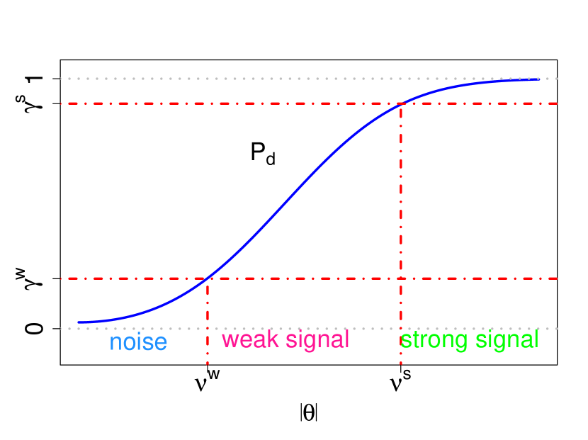
In the following, we define a strong signal if $P_{d}$ is close to 1, a noise variable if $P_{d}$ is close to 0, and a weak signal if a signal strength is in-between strong and noise levels. Specifically, suppose there are two threshold probabilities, $\gamma^{s}$ and $\gamma^{w}$ derived from $P_{d}$, the three signal-strength levels are defined as:

$$\begin{cases}\theta\in\bm{\Theta^{(S)}}&\mbox{ if }P_{d}>\gamma^{s}\\ \theta\in\bm{\Theta^{(W)}}&\mbox{ if }\gamma^{w}<P_{d}\leq\gamma^{s}\\ \theta\in\bm{\Theta^{(N)}}&\mbox{ if }P_{d}\leq\gamma^{w},\end{cases}$$ (3.2)

where $\tau_{0}\preceq\gamma^{w}<\gamma^{s}\preceq 1$, and $\tau_{0}=\min_{\theta}P_{d}(\theta)=2\Phi(-\frac{\sqrt{n\lambda}}{\sigma})$ can be viewed as a false-positive rate of model selection. Theoretically $\tau_{0}\rightarrow 0$ when $n\rightarrow\infty$ for consistent model selection. In finite samples, $\tau_{0}$ does not need to be 0, but close to 0.

To see the connection between signal detectability $P_{d}$ and signal strength, we let $\nu^{\gamma}$ be a positive solution of $P_{d}=\gamma$ in (3.1):

$$\gamma=\Phi(\frac{\nu^{\gamma}-\sqrt{\lambda}}{\sigma/\sqrt{n}})+\Phi(\frac{-\nu^{\gamma}-\sqrt{\lambda}}{\sigma/\sqrt{n}}).$$ (3.3)

It can be shown that $\nu^{\gamma}$ is an increasing function of $\gamma$. In addition, if the two positive threshold values $\nu^{s}$ and $\nu^{w}$ are solutions of equation (3.3) corresponding to $\gamma=\gamma^{s}$ and $\gamma^{w}$, then the definition in (3.2) is equivalent to

$$\begin{cases}\theta\in\bm{\Theta^{(S)}}&\mbox{ if }|\theta|>\nu^{s}\\ \theta\in\bm{\Theta^{(W)}}&\mbox{ if }\nu^{w}<|\theta|\leq\nu^{s}\\ \theta\in\bm{\Theta^{(N)}}&\mbox{ if }|\theta|\leq\nu^{w}.\end{cases}$$ (3.4)

Figure 2 also illustrates a connection between definition (3.2) and definition (3.4).

The following lemma provides selections of $\gamma^{s}$ and $\gamma^{w}$, which is useful to differentiate weak signals from noise variables. Lemma 1 also infers the order of weak signals, given both $\gamma^{s}$ and $\gamma^{w}$ are bounded away from 0 and 1.

Lemma 1.

(Selection of $\gamma^{s}$ and $\gamma^{w}$) If assumptions of $\sqrt{n}\lambda_{n}\rightarrow 0,n\lambda_{n}\rightarrow\infty$ are satisfied, and if the threshold values of detectability $\gamma^{w}$ and $\gamma^{s}$ corresponding to the lower bounds of weak and strong signals satisfy:

$$\max\left\{\epsilon,2\Phi(-\frac{\sqrt{n\lambda_{n}}}{\sigma})\right\}<\gamma^{w}<\gamma^{s}<1-\epsilon,$$

where $\epsilon$ is a small positive value; then for any $\gamma$ in the weak signal range $(\gamma^{w},\gamma^{s})$, we have $\nu^{\gamma}/\sqrt{\lambda_{n}}\rightarrow 1$.

Although Lemma 1 implies that $\nu$ within the weak signal range converges to zero asymptotically, the weak signal and noise variables have different orders. Specifically, Lemma 1 indicates that if the regularity condition $n\lambda_{n}\rightarrow\infty$ is satisfied, then a weak signal goes to zero more slowly than a noise variable. This is due to the fact that the weak signal has the same order as $\sqrt{\lambda_{n}}$, which goes to zero more slowly than the order of noise level $n^{-1/2}$. To simplify notation, the tuning parameter $\lambda_{n}$ is denoted as $\lambda$ throughout the rest of the paper.

The definitions in (3.2) and (3.4) are particularly meaningful in finite samples since $\nu^{\gamma}$ depends on $n,\lambda,\sigma$ and $\gamma$. That is, the weak signals are relative and depend on the sample size, the signal to noise ratio, and the tuning parameter selection. In other words, weak signals $\bm{\Theta^{(W)}}$ might be asymptotically trivial since the three levels automatically degenerate into two levels: zero and nonzero coefficients. However, weak signals should not be ignored in finite samples and serve as a transition phase between noise variables $\bm{\Theta^{(N)}}$ and strong signals $\bm{\Theta^{(S)}}$.

3.2 Weak Signal Identification

In this section we discuss how to identify weak signals more specifically. We propose a two-step procedure to recover possible weak signals which might be missed in a standard model selection procedure, and distinguish weak signals from strong signals.

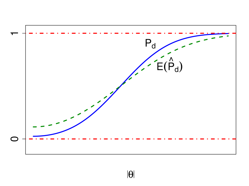
The key component of the proposed procedure is to utilize the estimated probability of detection $\widehat{P}_{d}$. Since the true information of parameter $\theta$ is unknown, $P_{d}$ cannot be calculated directly using (3.1). We propose to estimate $P_{d}$ by plugging in the least-square estimator $\hat{\theta}_{LS}$ in (3.1). The expectation of the estimator $\widehat{P}_{d}$ remains an increasing function of $|\theta|$. That is,

$$\widehat{P}_{d}=\Phi(\frac{\hat{\theta}_{LS}-\sqrt{\lambda}}{\sigma/\sqrt{n}})+\Phi(\frac{-\hat{\theta}_{LS}-\sqrt{\lambda}}{\sigma/\sqrt{n}}),$$ (3.5)

and

$$E(\widehat{P}_{d})=\Phi(\frac{\sqrt{n}}{\sqrt{2}\sigma}(\theta-\sqrt{\lambda}))-\Phi(-\frac{\sqrt{n}}{\sqrt{2}\sigma}(\theta+\sqrt{\lambda})).$$

In the following, the weak signal is identified through replacing $P_{d},(\gamma^{w},\nu^{w})$ and $(\gamma^{s},\nu^{s})$ in (3.2) by $\widehat{P}_{d},(\gamma_{1},\nu_{1})$ and $(\gamma_{2},\nu_{2})$, where $(\gamma_{1},\nu_{1})$ and $(\gamma_{2},\nu_{2})$ satisfy equation (3.3). We denote the identified noise, weak and strong signal set as $\left(\widehat{\bm{S}}^{\bm{(N)}},\bm{\widehat{S}^{(W)}},\bm{\widehat{S}^{(S)}}\right)$, where

$$\widehat{\bm{S}}^{\bm{(N)}} = \left\{i:|\hat{\theta}_{LS,i}|\leq\nu_{1},i=1,\cdots,p\right\}=\left\{i:\widehat{P}_{d,i}\leq\gamma_{1}\right\},$$

$$\widehat{\bm{S}}^{\bm{(W)}} = \left\{i:\nu_{1}<|\hat{\theta}_{LS,i}|\leq\nu_{2},i=1,\cdots,p\right\}=\left\{i:\gamma_{1}<\widehat{P}_{d,i}\leq\gamma_{2}\right\},\mbox{ and}$$

$$\widehat{\bm{S}}^{\bm{(S)}} = \left\{i:|\hat{\theta}_{LS,i}|>\nu_{2},i=1,\cdots,p\right\}=\left\{i:\widehat{P}_{d,i}>\gamma_{2}\right\}.$$

The details of selecting $\nu_{1}$ and $\nu_{2}$ are given below.

Note that in finite samples, there is no ideal threshold value $\nu_{1}$ which can separate signal variables and noise variables perfectly, as there is a trade-off between recovering weak signals and including noise variables. Here $\nu_{1}$ is selected to control a signal’s false-positive rate $\tau$. Specifically, $\nu_{1}=z_{\tau/2}\frac{\sigma}{\sqrt{n}}$ for any given tolerant false-positive rate $\tau$ since it can be shown that $P(i\notin\widehat{\bm{S}}^{\bm{(N)}}|\theta_{i}=0)=\tau,$ see Lemma 3 in the Appendix. Here we choose the false-positive rate $\tau$ to be larger than the $\tau_{0}$, since we intend to recover most of the weak signals. This is very different from standard model selection which mainly focuses on model selection consistency, but neglects detection of weak signals.

The low threshold value $\nu_{2}$ for strong signals is selected to ensure that a strong signal can be identified with high probability. We choose $\nu_{2}=\sqrt{\lambda}+z_{\alpha/2}\frac{\sigma}{\sqrt{n}}$, and it can be verified that the estimated detection rate $\widehat{P}_{d}$ for any identified strong signal stays above $1-\alpha$. In fact, based on (3.5), $\widehat{P}_{d}$ satisfies the inequality $P_{d}>E(\widehat{P}_{d})$ when the true signal is strong. Figure 2 illustrates the relationship between $P_{d}$ and $E(\widehat{P}_{d})$. Therefore there is a high probability that the true detection rate $P_{d}$ is larger than $1-\alpha$ when $\widehat{P}_{d}>1-\alpha$.

Figure 1: Define signal level based on $P_{d}$

Figure 2: $P_{d}$ and $E(\widehat{P}_{d})$

In summary, the main focus of weak signal identification is to recover weak signals as much as possible, at the cost of having a false-positive rate $\tau$ in finite samples. This is in contrast to standard model selection procedures which emphasize consistent model selection with a close-to-zero false-positive rate, but at the cost of not selecting most weak signals.

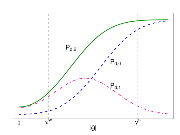
To better understand the difference and connection between the proposed weak signal identification procedure and the standard model selection procedure, we provide Figure 3 for illustration. Let $P_{d,0}(\theta)$ (dashed line) and $P_{d,1}(\theta)$ (dotted line) denote the probabilities of selecting $\theta$ in the standard model selection and the proposed weak signal identification, respectively, where $P_{d,0}(\theta)=P(|\hat{\theta}_{LS}|>\sqrt{\lambda})$, and $P_{d,1}(\theta)=P(\nu_{1}<|\hat{\theta}_{LS}|<\sqrt{\lambda})$. Then the total selection probability $P_{d,2}(\theta)$ (solid line) for the proposed method is $P_{d,2}(\theta)=P_{d,0}(\theta)+P_{d,1}(\theta)=P(|\hat{\theta}_{LS}|>\nu_{1}).$ Figure 3 indicates that the proposed procedure recovers weak signals better than the standard model selection procedure, but at a cost of a small false-positive rate of including some noise variables. These two procedures have similar detection power for strong signals.

Figure 3: Signal’s detectability in two-step procedure

4 Weak Signal Inference

4.1 Two-Step Inference Method

In this section, we propose a two-step inference procedure which consists of an asymptotic-based confidence interval for strong signals, and a least-square confidence interval for the identified weak signals. In the following, the proposed procedure is based on the orthogonal design assumption.

The asymptotic-based inference method has been developed for the SCAD estimator ([6]). [34] also provides the asymptotic distribution of the adaptive Lasso estimator $\widehat{\bm{\theta}}_{\bm{\mathcal{A}_{n}}}$ for nonzero parameters, where $\mathcal{A}_{n}=\{1,2,\cdots,q\}$. In finite samples, the adaptive Lasso estimator $\widehat{\bm{\theta}}_{\bm{\mathcal{A}_{n}}}$ is biased due to the shrinkage estimation. The bias term of $\widehat{\bm{\theta}}_{\bm{\mathcal{A}_{n}}}$ and the covariance matrix estimator of $\widehat{\bm{\theta}}_{\bm{\mathcal{A}_{n}}}$ are given by

$$\bm{\hat{b}}(\widehat{\bm{\theta}}_{\mathcal{A}_{n}})=(\frac{1}{n}\bm{X_{\mathcal{A}_{n}}}^{T}\bm{X_{\mathcal{A}_{n}}})^{-1}(p_{\lambda}^{{}^{\prime}}(|\hat{\theta}_{1}|)sgn(\hat{\theta}_{1}),\cdots,p_{\lambda}^{{}^{\prime}}(|\hat{\theta}_{q}|)sgn(\hat{\theta}_{q}))^{T},$$ (4.1)

and

$$\widehat{Cov}(\bm{\widehat{\theta}_{\mathcal{A}_{n}}})=\left\{\bm{X_{\mathcal{A}_{n}}}^{T}\bm{X_{\mathcal{A}_{n}}}+n\lambda\bm{\Omega}\right\}^{-1}\bm{X_{\mathcal{A}_{n}}}^{T}\bm{X_{\mathcal{A}_{n}}}\ \left\{\bm{X_{\mathcal{A}_{n}}}^{T}\bm{X_{\mathcal{A}_{n}}}+n\lambda\bm{\Omega}\right\}^{-1}\widehat{\sigma}^{2},$$ (4.2)

where $\bm{\Omega}=\mbox{diag}\left\{\frac{\hat{w}_{1}}{|\hat{\theta}_{1}|},\cdots,\frac{\hat{w}_{q}}{|\hat{\theta}_{q}|}\right\}$, and $\hat{w}_{i}=1/|\hat{\theta}_{LS,i}|$. Although the bias term is asymptotically negligible, it is important to correct the biased term to get more accurate confidence intervals in finite samples.

Consequently, if the $i$th variable is identified as a strong signal in $\widehat{\bm{S}}^{\bm{(S)}}$, a $100(1-\alpha)\%$ confidence interval for $\theta_{i}$ can be constructed as

$$\hat{\theta}_{i}+\hat{b}_{AL,i}\pm z_{\alpha/2}\hat{\sigma}_{AL,i},$$ (4.3)

where $\hat{b}_{AL,i}$ and $\hat{\sigma}_{AL,i}$ are the corresponding biased component in (4.1) and the square root of the diagonal variance component in (4.2), respectively. Under the orthogonal design, they are equivalent to

$$\hat{b}_{AL,i}=\frac{\lambda}{|\hat{\theta}_{LS,i}|}\cdot sgn(\hat{\theta}_{i}),$$ (4.4)

$$\mbox{and }\hat{\sigma}_{AL,i}=(1+\frac{\lambda}{|\hat{\theta}_{i}||\hat{\theta}_{LS,i}|})^{-1}\cdot\hat{\sigma}/n.$$ (4.5)

The above inference procedure performs well for strong signals ([6], [34] and [12]). However, this procedure does not apply well to weak signals. This is because weak signals are often missed in standard model selection procedures, and therefore there is no confidence interval constructed for any estimator shrunk to 0. Moreover, even if a weak signal is selected, the variance estimator in (4.2) tends to underestimate its true standard error, and consequently the confidence interval based on (4.3) is under-covered. Here we propose an alternative confidence interval for a weak signal in $\widehat{\bm{S}}^{\bm{(W)}}$ by utilizing the least-square information as follows.

The proposed inference for weak signals is motivated in that the bias-corrected confidence interval in (4.3) is close to the least-square confidence interval when a signal is strong. Therefore it is natural to construct a least-square confidence interval for a weak signal to solve the problem of excessive shrinkage for weak signal estimators.

If the $i$th variable is identified as a weak signal in $\widehat{\bm{S}}^{\bm{(W)}}$, we construct a $100(1-\alpha)\%$ least-square confidence interval for $\theta_{i}$ as

$$\hat{\theta}_{LS,i}\pm z_{\alpha/2}\hat{\sigma}_{LS,i},$$ (4.6)

where $\hat{\theta}_{LS,i}$ and $\hat{\sigma}_{LS,i}$ are the components of the least-square estimator and the square root of the diagonal component of the covariance matrix estimator:

$$\widehat{\bm{\theta}}_{\bm{LS}}=(\bm{X}^{T}\bm{X})^{-1}\bm{X}^{T}\bm{y},$$

$$\widehat{Cov}(\bm{\widehat{\theta}_{LS}})=(\bm{X}^{T}\bm{X})^{-1}\widehat{\sigma}^{2}.$$

Under the orthogonal design, $\hat{\theta}_{LS,i}$ and $\hat{\sigma}_{LS,i}$ are

$$\hat{\theta}_{LS,i}=\bm{X}_{i}^{T}\bm{y}/n,$$

$$\hat{\sigma}_{LS,i}=\hat{\sigma}/n.$$

In summary, if a non-zero signal is detected, combining (4.3) and (4.6), we provide a new two-step confidence interval for the $i$th variable as follows:

$$\left\{\hat{\theta}_{LS,i}\pm z_{\alpha/2}\hat{\sigma}_{LS,i}\right\}\mathbf{1}_{\left\{\mbox{$i\in\widehat{\bm{S}}^{\bm{(W)}}$}\right\}}+\left\{\hat{\theta}_{i}+\hat{b}_{AL,i}\pm z_{\alpha/2}\hat{\sigma}_{AL,i}\right\}\mathbf{1}_{\left\{\mbox{$i\in\widehat{\bm{S}}^{\bm{(S)}}$}\right\}}.$$

Here we propose different confidence interval constructions for weak and strong signals, and the proposed inference is a mixed procedure combining (4.3) and (4.6). Our inference procedure performs similarly to the asymptotic inference for strong signals, but outperforms the existing inference procedures in that the proposed confidence interval provides more accurate coverage for weak signals. Note that if a signal strength is too weak, neither existing methods nor our method can provide reasonably good inferences. Nevertheless, our method still provides a better inference than the asymptotic-based method across all signal levels.

4.2 Finite Sample Theories

In this section, we establish finite sample theory on coverage rate for the proposed two-step inference method, and compare it with the coverage rate of the asymptotic-based inference method. The asymptotic properties for penalized estimators have been investigated by [6], [8], [34], [36] and many others. When the sample size is sufficiently large and the signal strength is strong, the asymptotic inference is quite accurate in capturing the information of the penalized estimators. For instance, the covariance estimator of the penalized estimates in (4.2) is a consistent estimator ([8]). However, the sandwich estimator of the covariance only performs well for strong signals, not for weak signals in finite samples. Therefore, it is important to investigate the finite sample property of the penalized estimator, and especially the weak signal estimators for the proposed method.

We construct the exact coverage rates of the $100(1-\alpha)\%$ confidence intervals for the proposed method and the asymptotic method when the sample size is finite. The derivation for finite sample theory is very different from the asymptotic theory. In addition, since the coverage rate function is not monotonic, we need to compare the difference of the two coverage rates piece-wisely.

Given a confidence level parameter $\alpha$, the following regularity conditions are required for selecting the false-positive rate $\tau$:

1. $\tau\geq\alpha$,

2. $\frac{\alpha+\tau}{2}<\Phi(-\frac{1}{2}z_{\alpha/2})$, which is equivalent to $\tau<2\Phi(-\frac{1}{2}z_{\alpha/2})-\alpha$.

Condition (C1) is to ensure that the second step of the proposed method is able to identify weak signals. Condition (C2) provides a range of $\tau,$ so the false positive-rate is not too large. In addition, we also assume that $\lambda$ satisfies the criterion:

$$\sqrt{\lambda}\geq z_{\alpha/2}\frac{\sigma}{\sqrt{n}}.$$ (4.7)

The criterion in (4.7) implies that our focus is the case when $\sqrt{\lambda}\geq z_{\alpha/2}\frac{\sigma}{\sqrt{n}}$, where excessive shrinkage might affect weak signal selection. It can be verified that $\alpha\geq\tau_{0}$ if $\lambda$ is in this range, and this guarantees that $\tau>\tau_{0}$.

In the following, for any parameter $\theta$ and parameter $\nu$ associated with a different level of tuning, we introduce three probability functions, $P_{s}$, $CR_{a}$ and $CR_{b}$ as follows. Let $P_{s}$ be the detection power of $\theta$:

$$P_{s}(\theta,\nu)=\Phi(\frac{\theta-\nu}{\sigma/\sqrt{n}})+\Phi(\frac{-\theta-\nu}{\sigma/\sqrt{n}}).$$

We define $CR_{a}$ as the coverage probability based on the asymptotic inference approach when $|\hat{\theta}_{LS}|$ is larger than $\nu$:

$$CR_{a}(\theta,\nu)=\begin{cases}\left\{P_{s}(\theta,\nu)-2\Phi(-z_{\alpha/2}\frac{\tilde{\sigma}(\theta)}{\sigma})\right\}\\ \cdot I_{\left\{\nu\leq z_{\alpha/2}\frac{\tilde{\sigma}(\theta)}{\sqrt{n}}\right\}}&\mbox{if }|\theta|\leq|\nu-z_{\alpha/2}\frac{\tilde{\sigma}(\theta)}{\sqrt{n}}|\\ \Phi(z_{\alpha/2}\frac{\tilde{\sigma}(\theta)}{\sigma})-\Phi(\frac{\sqrt{n}(\nu-\theta)}{\sigma})&\mbox{if }|\nu-z_{\alpha/2}\frac{\tilde{\sigma}(\theta)}{\sqrt{n}}|\leq|\theta|\leq\nu+z_{\alpha/2}\frac{\tilde{\sigma}(\theta)}{\sqrt{n}}\\ 1-2\Phi(-z_{\alpha/2}\frac{\tilde{\sigma}(\theta)}{\sigma})&\mbox{if }|\theta|>\nu+z_{\alpha/2}\frac{\tilde{\sigma}(\theta)}{\sqrt{n}},\end{cases}$$

where $\tilde{\sigma}(\theta)=(1+\frac{\lambda}{\theta^{2}})^{-1}\sigma$; and $CR_{b}$ is the coverage probability based on the least-square confidence interval when $|\hat{\theta}_{LS}|$ is larger than $\nu$:

$$CR_{b}(\theta,\nu)=\begin{cases}\left\{P_{s}(\theta,\nu)-\alpha\right\}\cdot I_{\left\{\nu\leq z_{\alpha/2}\frac{\sigma}{\sqrt{n}}\right\}}&\mbox{if }|\theta|\leq|\nu-z_{\alpha/2}\frac{\sigma}{\sqrt{n}}|\\ 1-\frac{\alpha}{2}-\Phi(\frac{\sqrt{n}(\nu-\theta)}{\sigma})&\mbox{if }|\nu-z_{\alpha/2}\frac{\sigma}{\sqrt{n}}|\leq|\theta|\leq\nu+z_{\alpha/2}\frac{\sigma}{\sqrt{n}}\\ 1-\alpha&\mbox{if }|\theta|>\nu+z_{\alpha/2}\frac{\sigma}{\sqrt{n}}.\end{cases}$$

The explicit expressions of coverage rates based on the asymptotic and the proposed two-step methods are provided in the following lemma.

Lemma 2.

Suppose $n,\sigma$ and tuning parameter $\lambda$ are given, the coverage rate $CR_{1}(\theta)$ of the $100(1-\alpha)\%$ confidence interval for any coefficient $\theta$ based on the asymptotic inference is

$$CR_{1}(\theta)=\frac{CR_{a}(\theta,\nu_{0})}{P_{s}(\theta,\nu_{0})},$$ (4.8)

where $\nu_{0}=\sqrt{\lambda}$. Given any $\tau$, the coverage rate $CR(\theta)$ of the $100(1-\alpha)\%$ confidence interval for any coefficient $\theta$ using the proposed two-step inference method is given by:

$$CR(\theta)=\frac{CR_{b}(\theta,\nu_{1})+CR_{a}(\theta,\nu_{2})-CR_{b}(\theta,\nu_{2})}{P_{s}(\theta,\nu_{1})},$$ (4.9)

where $\nu_{0}=\sqrt{\lambda},\nu_{1}=z_{\tau/2}\frac{\sigma}{\sqrt{n}}$, and $\nu_{2}=\sqrt{\lambda}+z_{\alpha/2}\frac{\sigma}{\sqrt{n}}.$

The derivations of $CR_{1}(\theta)$ and $CR(\theta)$ are provided in the proof of Lemma 2 in the Appendix. In fact, $CR_{1}(\theta)$ is the conditional coverage probability based on the asymptotic confidence interval, given that $\theta$ is selected using tuning parameter $\lambda$. Similarly, $CR(\theta)$ is the conditional coverage probability of the proposed confidence interval in (4.1), given that $\theta$ is selected based on the two-step procedure. The expression of $CR(\theta)$ in (4.9) can be interpreted as the summation of two sub-components, where the first component $\frac{CR_{b}(\theta,\nu_{1})-CR_{b}(\theta,\nu_{2})}{P_{s}(\theta,\nu_{1})}$, corresponds to the conditional coverage probability of the least-square confidence interval when $\nu_{1}<|\hat{\theta}_{LS}|<\nu_{2}$, and the second component $\frac{CR_{a}(\theta,\nu_{2})}{P_{s}(\theta,\nu_{1})}$, is the conditional coverage probability of the asymptotic-based confidence interval when $|\hat{\theta}_{LS}|>\nu_{2}$.

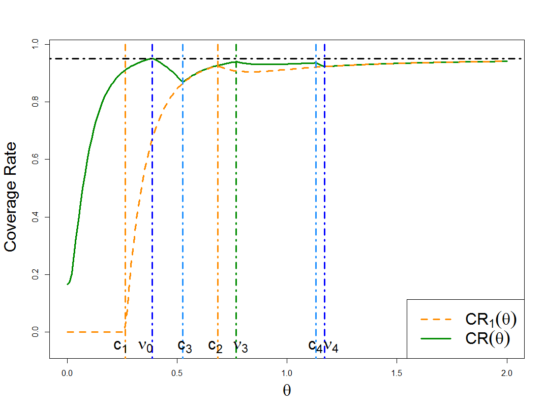
In addition, we show in the supplement that both $CR_{1}(\theta)$ and $CR(\theta)$ are piece-wise smooth functions, and require one to compare two coverage rates at each interval separately. We introduce the boundary points associated with $CR_{1}(\theta)$ and $CR(\theta)$ as follows. Let $c_{1}$, $c_{2}$, $c_{3}$ and $c_{4}$ be the solutions of $\theta=\sqrt{\lambda}-z_{\alpha/2}\frac{\tilde{\sigma}(\theta)}{\sqrt{n}}$, $\theta=\sqrt{\lambda}+z_{\alpha/2}\frac{\tilde{\sigma}(\theta)}{\sqrt{n}}$, $\theta=\sqrt{\lambda}+z_{\alpha/2}\frac{\sigma}{\sqrt{n}}-z_{\alpha/2}\frac{\tilde{\sigma}(\theta)}{\sqrt{n}}$, and $\theta=\sqrt{\lambda}+z_{\alpha/2}\frac{\sigma}{\sqrt{n}}+z_{\alpha/2}\frac{\tilde{\sigma}(\theta)}{\sqrt{n}}$, respectively. Here $c_{1}$ and $c_{2}$ are the boundary points of piece-wise intervals for $CR_{1}(\theta)$ in (4.8), and $c_{3}$ and $c_{4}$ are the boundary points of piece-wise intervals for $CR(\theta)$ in (4.9). It can be shown that the orders of $c_{1},c_{2},c_{3}$ and $c_{4}$ satisfy $c_{1}<c_{3}<c_{2}<c_{4}.$ More specific ranges for $c_{1},$ $c_{2}$, $c_{3}$ and $c_{4}$ are provided in Lemma 4 of the Appendix. Since there are no explicit solutions for these boundary points, we rely on the orders of these boundary points to examine the difference between $CR_{1}(\theta)$ and $CR(\theta)$.

In the following, we define $\Delta(\theta)=CR(\theta)-CR_{1}(\theta)$ as a difference function between $CR(\theta)$ and $CR_{1}(\theta)$. Theorem 1 and Theorem 2 provide the uniform low bounds of $\Delta(\theta)$ for different ranges of $\lambda$ when $z_{\alpha/2}\frac{\sigma}{\sqrt{n}}\leq\sqrt{\lambda}<(z_{\alpha/2}+z_{\tau/2})\frac{\sigma}{\sqrt{n}}$ and $\sqrt{\lambda}\geq(z_{\alpha/2}+z_{\tau/2})\frac{\sigma}{\sqrt{n}}$. The mathematical details of the proofs are provided in the Appendix and supplement materials.

Theorem 1.

Under conditions (C1)-(C2), if $\lambda$ satisfies $z_{\alpha/2}\frac{\sigma}{\sqrt{n}}<\sqrt{\lambda}<(z_{\alpha/2}+z_{\tau/2})\frac{\sigma}{\sqrt{n}}$, the piece-wise lower bounds for $\Delta(\theta)$ are provided as follows:

1. when $\theta\in\left[0,c_{1}\right],$ $\Delta(\theta)\geq 1-\frac{\alpha}{\tau}>0;$

2. when $\theta\in\left[c_{1},\nu_{0}\right],$ $\Delta(\theta)\geq\frac{2}{1+\alpha}-2\Phi(\frac{1}{2}z_{\alpha/2})>0;$

3. when $\theta\in\left[\nu_{0},+\infty\right),$ $\Delta(\theta)$ satisfies either $\Delta(\theta)\geq 0$ or $-\frac{\alpha}{2}<\Delta(\theta)<0$.

In addition, a more specific lower bound for $\Delta(\theta)$ on $\left[\nu_{0},+\infty\right)$ is given by:

$$\Delta(\theta)\geq\begin{cases}-4(1-\frac{\alpha}{2})\Phi(-\frac{3}{2}z_{\alpha/2})&\mbox{if }\theta\in\left[\nu_{0},\min\left\{\nu_{3},c_{3}\right\}\right]\\ \mbox{ See Table \ref{tab:threecase}}&\mbox{if }\theta\in\left[\min\left\{\nu_{3},c_{3}\right\},\max\left\{\nu_{3},c_{2}\right\}\right]\\ -\frac{4(1-\alpha)}{(2-\alpha)^{2}}\Phi(-2z_{\alpha/2})-\frac{\alpha(1-\alpha)}{2-\alpha}&\mbox{if }\theta\in\left[\max\left\{\nu_{3},c_{2}\right\},c_{4}\right]\\ -(1-\alpha)\frac{\Phi(-\frac{3}{2}z_{\alpha/2})}{\Phi(\frac{3}{2}z_{\alpha/2})^{2}}&\mbox{if }\theta\in\left[c_{4},\nu_{4}\right]\\ -(1-\alpha)\frac{\Phi(-2z_{\alpha/2})}{\Phi(2z_{\alpha/2})^{2}}&\mbox{if }\theta\in\left[\nu_{4},\infty\right),\\ \end{cases}$$

where $\nu_{3}=(z_{\alpha/2}+z_{\tau/2})\frac{\sigma}{\sqrt{n}}$, and $\nu_{4}=\sqrt{\lambda}+2z_{\alpha/2}\frac{\sigma}{\sqrt{n}}.$ Table 1 provides the lower bounds for $\Delta(\theta)$ on interval $\left[\min\left\{\nu_{3},c_{3}\right\},\max\left\{\nu_{3},c_{2}\right\}\right]$ under three cases.

Table 1: Specific bounds of $\Delta(\theta)$ on interval $\left[\min\left\{\nu_{3},c_{3}\right\},\max\left\{\nu_{3},c_{2}\right\}\right]$

case 1:	$\theta\in\left[c_{3},\nu_{3}\right]$	$\theta\in\left[\nu_{3},c_{2}\right]$
$c_{3}<\nu_{3}<c_{2}$	$-2\Phi(-\frac{3}{2}z_{\alpha/2})$	$-\frac{4(1-\alpha)}{(2-\alpha)^{2}}\Phi(-2z_{\alpha/2})-\frac{\alpha(1-\alpha)}{2-\alpha}$
case 2:	$\theta\in\left[c_{3},c_{2}\right]$	$\theta\in\left[c_{2},\nu_{3}\right]$
$c_{3}<c_{2}<\nu_{3}$	$-2(1-\alpha)\Phi(-\frac{3}{2}z_{\alpha/2})$	$-\frac{1-\alpha}{\left[\Phi(\frac{1}{2}z_{\alpha/2})\right]^{2}}\Phi(-2z_{\alpha/2})$
case 3:	$\theta\in\left[\nu_{3},c_{2}\right]$
$\nu_{3}<c_{3}<c_{2}$	$-\frac{\alpha}{2}$

Theorem 2.

Under conditions (C1)-(C2), if $\lambda$ satisfies $\sqrt{\lambda}\geq(z_{\alpha/2}+z_{\tau/2})\frac{\sigma}{\sqrt{n}}$, the lower bounds for $\Delta(\theta)$ are provided as follows:

1. when $\theta\in\left[0,\min\left\{\nu_{3},c_{1}\right\}\right],$ $\Delta(\theta)\geq 1-\frac{\alpha}{\tau}>0;$

2. when $\theta\in\left[\min\left\{\nu_{3},c_{1}\right\},\nu_{0}\right],$ see Table 2;

3. when $\theta\in\left[\nu_{0},+\infty\right),$ $\Delta(\theta)\geq 0$ or $-\frac{\alpha}{2}<\Delta(\theta)<0$.

Table 2: Specific bounds of $\Delta(\theta)$ on interval $\left[\min\left\{\nu_{3},c_{1}\right\},\nu_{0}\right]$

case 4:	$\theta\in\left[\nu_{3},\nu_{0}\right]$
$\nu_{3}<c_{1}$	$2-\alpha-2\Phi(\frac{1}{2}z_{\alpha/2})$
case 5:	$\theta\in\left[c_{1},\nu_{3}\right]$	$\theta\in\left[\nu_{3},\nu_{0}\right]$
$c_{1}<\nu_{3}$	$\Phi(-\frac{1}{2}z_{\alpha/2})-\frac{\alpha}{2}$	$2-\alpha-2\Phi(\frac{1}{2}z_{\alpha/2})$

Theorem 1 and Theorem 2 indicate that the proposed method outperforms the asymptotic-based method, with a uniform lower bound for $\Delta(\theta)$ when $\theta\in\left[0,\nu_{0}\right]$. More specifically, the lower bound of $\Delta(\theta)$ depends on $\alpha$ and $\tau$ for case (i) $(\theta\in\left[0,c_{1}\right])$ in Theorem 1 and case (i) $(\theta\in\left[0,\min\left\{\nu_{3},c_{1}\right\}\right])$ in Theorem 2. Since we select $\tau$ to be larger than $\alpha,$ it is clear that $\Delta(\theta)$ is bounded above zero. For case (ii) $(\theta\in\left[c_{1},\nu_{0}\right])$ in Theorem 1 and case (ii) $(\theta\in\left[\min\left\{\nu_{3},c_{1}\right\},\nu_{0}\right])$ in Theorem 2, the lower bound of $\Delta(\theta)$ only depends on $\alpha$. In fact, the minimum value of $\frac{2}{1+\alpha}-2\Phi(\frac{1}{2}z_{\alpha/2})$ is larger than $0.22$ if $\alpha\in\left[0.05,0.1\right]$, based on Theorem 1. This also confirms that the proposed method provides a confidence region with at least 22% improvement in coverage rate than the one based on the asymptotic method. The lower bounds of case (ii) in Theorem 2 can be interpreted in a similar way.

In addition, both Theorem 1 and Theorem 2 imply that when $\theta\in\left(\nu_{0},+\infty\right)$ with a moderately large coefficient, the proposed method performs better than, or close to, the asymptotic method. In summary, the two-step inference method provides more accurate coverage than the one based on the asymptotic inference, and is also more effective for the weak signal region.

In Theorem 1, since the order relationships among $c_{2},c_{3}$ and $\nu_{3}$ change for different ranges of tuning parameters and choices of false positive rate $\tau$, it leads to the three cases in Table 1. Similarly, the order relationships among $\nu_{3}$ and $c_{1}$ also change for different choices of $\lambda$ and $\tau$ in Theorem 2, leading to the two cases in Table 2. Figure 4 illustrates an example for case 1. Figures for the other four cases are provided in the supplemental material.

Figure 4: $CR(\theta)$ versus $CR_{1}(\theta)$ (An example: Case 1)

5 Finite Sample Performance

5.1 Simulation Studies

To examine the empirical performance of the proposed inference procedure, we conduct simulation studies to evaluate the accuracy of the confidence intervals described in section 4.1. We generate $400$ simulated data with a sample size of $n$ under the linear model $y=\bm{X}\bm{\theta}+\mathcal{N}(0,\sigma^{2}),$ where $\bm{X}=(\bm{X}_{1},\cdots,\bm{X}_{p})$ and $\bm{X}_{j}\sim\mathcal{N}(\bm{0},\bm{I_{n}}).$ We allow covariates $\bm{X}$ to be correlated with an AR(1) correlation structure, and the pairwise correlation $cor(\bm{X_{i},X_{j}})=\rho^{|i-j|}.$ We choose $(n,p,\sigma)=(100,20,2)$ and $(400,50,2)$, and $\rho=0,0.2$ or $0.5$ for each setting. In addition, the $p$-dimensional coefficient vector $\bm{\theta}=(1,1,0.5,\theta,0,\cdots,0)$, which consists of two strong signals of 1’s, one moderate strong signal of 0.5, one varying-signal $\theta$, and $(p-4)$ null variables. We let the coefficient $\theta$ vary between 0 (null) to 1 (strong signal) to examine the confidence coverages across different signal strength levels.

We construct $95\%$ confidence intervals for an identified signal based on (4.1). We implement the glmnet package in R ([9]) to obtain the adaptive Lasso estimator. We choose the tuning parameter $\lambda$ based on the Bayesian information criterion (BIC), because of its consistency property to select the true model ([30]). Here we follow a strategy by [28] to select the BIC tuning parameter for the adaptive Lasso penalty (details are provided in Appendix A.2). The standard deviation $\hat{\sigma}$ is estimated based on the scaled Lasso method ([25]), using the ‘scalreg’ package in R. We replace $\hat{\theta}_{i}$ by its bias-corrected form $\hat{\theta}_{i}+\hat{b}_{AL,i}$ in (4.5) when estimating $\hat{\sigma}_{AL}$, which achieves better estimation of the true standard deviation. For comparison, we also construct standard confidence intervals based on the asymptotic formula in (4.3), along with the bootstrap method ([5]), the smoothed bootstrap method ([4]), the perturbation method ([19]), and the de-biased Lasso method ([13]). The de-biased method is implemented using the R codes provided by Montanari’s website. For both regular bootstrap and smoothed bootstrap methods, the number of bootstrap sampling is set to be $4000$ ([4]). For the perturbation method, the resampling time is set to be $500$ according to [19].

In addition, the coverage rate for the OLS estimator is included as a benchmark since there is no shrinkage in OLS estimation and the confidence interval is the most accurate. Here the OLS estimator $\hat{\theta}_{LS}$ given in (4.6) is estimated from the full model. We used the estimator from the full model because our method assumes that the covariates are orthogonally designed. Under this assumption, the least square estimator under a submodel is the same estimator as that under the full model. If covariates are correlated, the estimator under the correctly specified submodel is more efficient than the one under the full model. However, we cannot guarantee that the selected submodel is correctly specified. If the submodel is misspecified, then the $\hat{\theta}_{LS}$ could be biased, which could lead to inaccurate inference for the coefficients of the selected variables. Note that selection of the wrong model is likely, especially when weak signals exist.

Figure 5 illustrates the relationship between $\tau_{0}$ and $\tau$ when $\rho=0.2$ for two model settings $(n,p,\sigma)=(100,20,2)$ and $(400,50,2)$, where $\tau_{0}=2\Phi(-\frac{\sqrt{n\lambda}}{\sigma})$ based on Section 3.1. We choose $\tau$ larger than $\tau_{0}$ according to Section 3.2, that is, the false-positive rate in the weak signal recovery procedure is slightly larger than the false-positive rate in the model selection procedure. In these two model settings, $\tau_{0}$ are around 0.1 and 0.03 respectively; here we select $\tau$ as 0.2. In practice, the selection of $\tau$ is flexible, and can be determined by a tolerance level for including noise variables.

Figure 5: False positive rate for simulation setting 1 (left) & 2 (right)

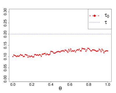
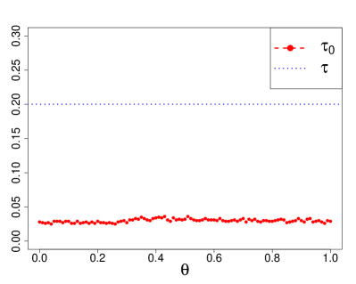
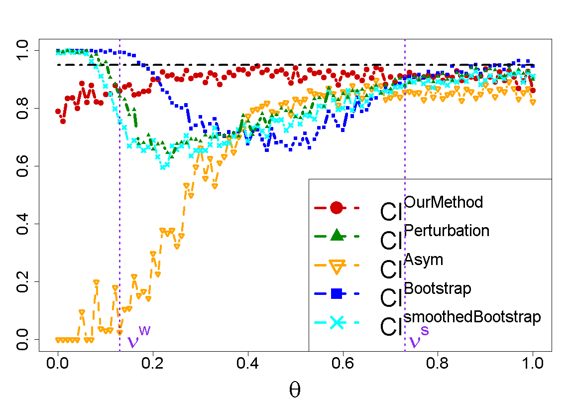
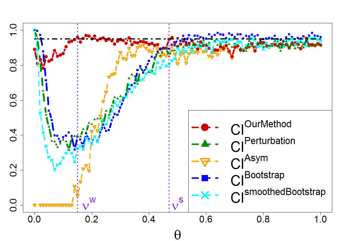
Figure 6 and Figure 7 provide the coverage probabilities for $\theta$ varying between 0 and 1 when $\rho=0.2$ in two model settings. In each figure, $\nu^{s}$ and $\nu^{w}$ are the average threshold coefficients corresponding to the detection powers $P_{d}=0.9$ and $0.1$, respectively. When the signal strength is close to zero, neither of the coverage rates using our method and the asymptotic method are accurate. However, the proposed method is still better than the asymptotic one, since the asymptotic coverage rate is close to zero; while the bootstrap and perturbation methods tend to provide over-coverage confidence intervals. The proposed method becomes more accurate as the magnitude of signal $\theta$ increases, and also outperforms all the other methods especially in the weak signal region. For example, in setting 1, the coverage rate of the proposed method is quite close to 95% when the signal strength is larger than 0.4. On the other hand, the resampling methods and asymptotic inference provide low coverage rates for signal strength below 0.8. When signal strength is above 0.8, the coverages from all methods are accurate and close to 95%.

Figure 6: 95% confidence interval’s coverage rates for simulation setting 1 when $\rho=0.2$

Figure 7: 95% confidence interval’s coverage rates for simulation setting 2 when $\rho=0.2$

Table 3: Coverage probabilities of confidence regions when $\sigma=2$

			p=20			p=50
n	$\theta$		$\rho=0$	$\rho=0.2$	$\rho=0.5$	$\rho=0$	$\rho=0.2$	$\rho=0.5$
100	0.3	$CR^{Our}$	94.4	92.6	91.1	92.1	91.1	95.3
		$CR^{Asym}$	61.5	61.2	38.3	33.3	18.5	21.4
		$CR^{Ptb}$	67.3	68.6	74.2	68.6	64.8	58.6
		$CR^{Bs}$	74.5	77.0	88.7	100.0*	100.0*	100.0*
		$CR^{smBS}$	68.1	65.4	74.3	95.1*	93.5*	92.3*
		$CR^{OLS}$	93.2	93.2	94.0	94.5	93.0	95.0
		$CR^{Lasso-debiased}$	94.5	95.5	97.0	94.8	94.0	96.5
	0.75	$CR^{Our}$	94.4	92.9	91.9	93.8	92.5	93.6
		$CR^{Asym}$	89.6	87.4	75.1	85.3	77.5	63.9
		$CR^{Ptb}$	87.6	90.9	86.4	90.0	93.8	78.9
		$CR^{Bs}$	91.4	90.7	88.0	98.9*	98.8*	100.0*
		$CR^{smBS}$	89.3	89.1	89.2	91.3*	95.3*	91.1*
		$CR^{OLS}$	92.8	96.0	94.0	95.5	95.5	94.0
		$CR^{Lasso-debiased}$	93.8	96.5	96.8	96.3	96.0	96.3
200	0.2	$CR^{Our}$	94.6	94.7	93.3	95.3	93.7	91.3
		$CR^{Asym}$	52.0	51.6	38.1	15.9	22.4	18.0
		$CR^{Ptb}$	61.4	65.3	69.4	48.1	44.2	49.3
		$CR^{Bs}$	58.5	58.1	72.8	56.1	61.0	63.5
		$CR^{smBS}$	54.7	50.5	62.6	46.0	48.8	46.4
		$CR^{OLS}$	95.2	94.2	95.8	95.2	95.5	95.8
		$CR^{Lasso-debiased}$	93.5	95.0	96.5	95.5	96.0	94.8
	0.6	$CR^{Our}$	95.5	93.0	91.5	93.7	91.6	90.3
		$CR^{Asym}$	88.8	86.2	76.6	88.5	82.7	65.0
		$CR^{Ptb}$	90.2	92.6	86.1	84.2	88.0	89.6
		$CR^{Bs}$	90.7	91.7	88.4	86.9	89.4	82.7
		$CR^{smBS}$	88.4	89.5	91.2	80.7	84.2	81.4
		$CR^{OLS}$	96.2	96.0	96.5	95.2	93.8	94.2
		$CR^{Lasso-debiased}$	95.5	95.3	96.3	95.0	95.0	94.0
400	0.15	$CR^{Our}$	93.6	94.6	93.4	97.0	96.3	90.5
		$CR^{Asym}$	31.7	33.8	44.8	9.1	11.6	10.7
		$CR^{Ptb}$	33.6	51.0	60.3	33.6	39.3	44.7
		$CR^{Bs}$	35.3	54.2	57.9	35.3	39.1	38.6
		$CR^{smBS}$	27.4	49.9	52.2	27.4	32.2	31.3
		$CR^{OLS}$	92.5	96.8	96.0	94.8	95.5	94.2
		$CR^{Lasso-debiased}$	90.8	93.3	91.5	94.0	96.5	93.0
	0.4	$CR^{Our}$	94.8	92.2	92.2	92.7	92.1	92.8
		$CR^{Asym}$	94.0	91.2	85.5	91.7	88.7	72.6
		$CR^{Ptb}$	79.5	89.3	89.2	79.5	75.8	70.7
		$CR^{Bs}$	87.5	89.3	80.3	87.5	82.4	70.3
		$CR^{smBS}$	79.8	87.2	84.3	79.8	76.6	71.0
		$CR^{OLS}$	95.8	93.2	93.5	94.5	94.8	93.0
		$CR^{Lasso-debiased}$	90.0	92.5	93.5	95.8	94.3	93.8

Note: The values are multiplied by 100. $*$ indicates that the bootstrap and smooth bootstrap methods encounter a singular-designed matrix problem (7-10% times), and only partial simulation results are used for calculation.

Table 4: Average widths of confidence intervals when $\sigma=2$

			p=20			p=50
n	$\theta$		$\rho=0$	$\rho=0.2$	$\rho=0.5$	$\rho=0$	$\rho=0.2$	$\rho=0.5$
100	0.3	len$CR^{Our}$	0.862	0.889	1.098	1.083	1.131	1.403
		len$CR^{Asym}$	0.594	0.593	0.582	0.542	0.541	0.519
		len$CR^{Ptb}$	0.652	0.691	0.803	0.679	0.672	0.829
		len$CR^{Bs}$	0.786	0.818	0.954	1.717*	1.756*	2.206*
		len$CR^{smBS}$	0.626	0.654	0.746	0.998*	1.014*	1.296*
		len$CR^{OLS}$	0.864	0.900	1.094	1.106	1.135	1.401
		len$CR^{Lasso-debiased}$	1.071	1.081	1.304	1.179	1.220	1.487
	0.75	len$CR^{Our}$	0.770	0.794	1.031	0.956	1.045	1.306
		len$CR^{Asym}$	0.659	0.659	0.648	0.612	0.592	0.579
		len$CR^{Ptb}$	0.911	0.929	1.129	0.973	0.971	1.154
		len$CR^{Bs}$	1.020	1.054	1.262	1.786*	1.886*	2.276*
		len$CR^{smBS}$	0.902	0.944	1.114	1.073*	1.134*	1.354*
		len$CR^{OLS}$	0.866	0.899	1.094	1.118	1.151	1.399
		len$CR^{Lasso-debiased}$	1.101	1.126	1.414	1.193	1.269	1.529
200	0.2	len$CR^{Our}$	0.580	0.603	0.743	0.628	0.659	0.812
		len$CR^{Asym}$	0.412	0.420	0.427	0.391	0.370	0.379
		len$CR^{Ptb}$	0.436	0.444	0.526	0.381	0.356	0.445
		len$CR^{Bs}$	0.458	0.504	0.586	0.470	0.504	0.600
		len$CR^{smBS}$	0.384	0.434	0.498	0.356	0.388	0.454
		len$CR^{OLS}$	0.581	0.603	0.745	0.635	0.658	0.815
		len$CR^{Lasso-debiased}$	0.635	0.681	0.817	0.838	0.832	0.845
	0.6	len$CR^{Our}$	0.517	0.567	0.700	0.556	0.614	0.765
		len$CR^{Asym}$	0.473	0.467	0.471	0.437	0.433	0.421
		len$CR^{Ptb}$	0.673	0.699	0.864	0.715	0.727	0.859
		len$CR^{Bs}$	0.714	0.734	0.902	0.814	0.820	0.992
		len$CR^{smBS}$	0.708	0.738	0.894	0.732	0.748	0.892
		len$CR^{OLS}$	0.584	0.604	0.743	0.641	0.661	0.818
		len$CR^{Lasso-debiased}$	0.689	0.728	0.933	0.865	0.862	0.866
400	0.15	len$CR^{Our}$	0.397	0.416	0.516	0.418	0.434	0.537
		len$CR^{Asym}$	0.293	0.296	0.311	0.283	0.283	0.278
		len$CR^{Ptb}$	0.309	0.312	0.391	0.226	0.247	0.261
		len$CR^{Bs}$	0.322	0.314	0.372	0.244	0.272	0.290
		len$CR^{smBS}$	0.308	0.298	0.352	0.214	0.242	0.254
		len$CR^{OLS}$	0.401	0.416	0.515	0.419	0.434	0.537
		len$CR^{Lasso-debiased}$	0.412	0.434	0.438	0.436	0.432	0.430
	0.4	len$CR^{Our}$	0.368	0.401	0.492	0.381	0.419	0.516
		len$CR^{Asym}$	0.327	0.329	0.337	0.306	0.303	0.306
		len$CR^{Ptb}$	0.507	0.531	0.638	0.545	0.552	0.602
		len$CR^{Bs}$	0.530	0.542	0.654	0.560	0.574	0.670
		len$CR^{smBS}$	0.578	0.596	0.712	0.578	0.600	0.698
		len$CR^{OLS}$	0.401	0.418	0.515	0.419	0.434	0.536
		len$CR^{Lasso-debiased}$	0.432	0.464	0.477	0.442	0.440	0.435

Note: $*$ indicates that the bootstrap and smooth bootstrap methods encounter a singular-designed matrix problem (7-10% times), and only partial simulation results are used for calculation.

The results for correlated covariates settings are provided in Table 3. For each setting, we select two different values of $\theta$ whose detection probabilities $P_{d}$ are between $0.1$ and $0.9$. Here the first $\theta$ is relatively weaker, and the second one is at the boundary of strong signal. For all these settings, the asymptotic inference, bootstrap and perturbation methods provide confidence intervals far below 95% when signals are weak. In general, our method provides a stable inference even when the correlation coefficient increases, and the coverage rate for weak signals is between 90-96% when $\rho=0.5$. The asymptotic-based inference has the lowest coverage rates among all, and performs extremely poorly when $\rho$ is larger. The coverage rates based on the perturbation method are all below 75% for weak signals. Note that the coverage rate improvement using the smoothed bootstrap method is not significant compared to the standard bootstrap method. In addition, for $n=100,p=50$, the bootstrap and smooth bootstrap methods face a singular-designed matrix problem due to small sample size, which does not produce any simulation results 7-10% of the time. The average coverage rates provided in Table 3 might not be valid and are marked with $*$.

Table 4 provides the CI lengths of all methods for both weak and strong signals. In general, the proposed method provides narrower confidence intervals and better coverage rates than the perturbation and bootstrap methods, and shorter confidence intervals with comparable coverage rates as the de-biased Lasso method for strong signals. For example, when $(n,p,\rho)=(100,20,0)$ and $\theta=0.75$, the coverage rate of our method is $94.4\%$, compared to $87.6\%$ based on the perturbation method, $91.4\%$ based on the bootstrap method, and 93.8% based on the de-biased method. The corresponding CI length of our method equals $0.770$, which is smaller than the $0.911$ from the perturbation method, $1.020$ from the bootstrap method, and 1.101 from the de-biased method. Furthermore, our CI is also shorter compared to the least square CI for strong signals in general.

For weak signals, our CI is wider than the perturbation and bootstrap methods. This is because both the perturbation and bootstrap methods provide inaccurate coverage rates which tend to be smaller than 95%. For example, when $(n,p,\rho)=(100,20,0)$ and $\theta=0.3$, the coverage rate of our method is $94.4\%$, compared to $67.3\%$ based on the perturbation method, $74.5\%$ based on the bootstrap method, and $94.5\%$ based on the de-biased Lasso method. The corresponding CI length of our method is $0.862$, which is wider than the $0.652$ from the perturbation method and the $0.786$ from the bootstrap method, but is still shorter than the $1.071$ from the de-biased Lasso method.

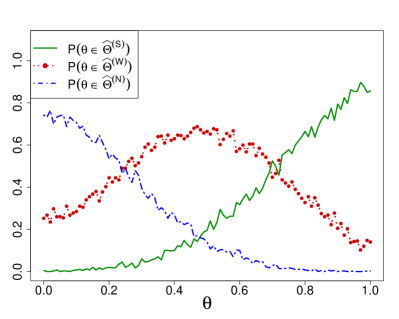
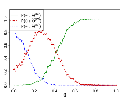
Figure 8 also presents the probabilities of assigning each signal category for a given $\theta$ value, where the probabilities for identified strong signal ($P(i\in\widehat{\bm{S}}^{\bm{(S)}})$), weak signal ($P(i\in\widehat{\bm{S}}^{\bm{(W)}})$) and null variable ($P(i\in\widehat{\bm{S}}^{\bm{(N)}})$) are denoted as solid, dotted and dashed lines, respectively. Here $i$ corresponds to the index of coefficient $\theta$. The probability of each identified signal category relies on signal strength. Specifically, when a signal is close to zero, it is likely to be identified as zero most of the time, with the highest $P(i\in\widehat{\bm{S}}^{\bm{(N)}})$; when a signal falls into the weak signal region, $P(i\in\widehat{\bm{S}}^{\bm{(W)}})$ becomes dominant; and when $\theta$ increases to be a strong signal, $P(i\in\widehat{\bm{S}}^{\bm{(S)}})$ also gradually increases and reaches to 1.

Figure 8: Empirical probabilities of identifying each signal level. Left: setting 1. Right: setting 2.

5.2 HIV Data Example

In this section, we apply HIV drug resistance data
(http://hivdb.stanford.edu/) to illustrate the proposed method. The HIV drug resistance study aims to identify the association of protease mutations with susceptibility to the antiretroviral drug. Since antiretroviral drug resistance is a major obstacle to the successful treatment of HIV-1 infection, studying the generic basis of HIV-1 drug resistance is crucial for developing new drugs and designing an optimal therapy for patients. The study was conducted on 702 HIV-infected patients, where 79 out of 99 protease codons in the viral genome have mutations. Here the drug resistance is measured in units of IC₅₀.

We consider a linear model:

$$\bm{y}=\sum_{i=1}^{p}\bm{X_{i}}\theta_{i}+\bm{\varepsilon},$$ (5.1)

where the response variable $\bm{y}$ is the log-transformation of nonnegative IC₅₀, and the model predictors $\bm{X_{i}}$ are binary variables indicating the mutation presence for each codon. For each predictor, $1$ represents mutation and $0$ represents no mutation. The total number of candidate codons $p=79$. We are interested in examining which codon mutations have effect on drug resistance.

We apply the proposed two-step inference method to identify codons’ mutation presence which have strong or mild effects on HIV drug resistance. We use the GLMNET in R to obtain the adaptive Lasso estimator for the linear model in (5.1), where the initial weight of each coefficient is based on the OLS estimator. The tuning parameter $\lambda$ is selected by the Bayesian information criterion, and $\sigma$ is estimated similarly as in [34]. To control the noise variable selection, we choose $\tau=0.05$. According to the proposed identification procedure in Section 3.2, we calculate two threshold values $\nu_{1}$ and $\nu_{2}$ as $0.061$ and $0.136$, which correspond to two threshold probabilities, $\gamma_{1}=0.327$ and $\gamma_{2}=0.975$, for identifying weak and strong signals, respectively.

We constructed 95% confidence intervals using the proposed method and the perturbation approach ([19]) for the chosen variables. Both the standard bootstrap and smoothed bootstrap methods are not applicable to the HIV data. Since mutation is rather rare and only a few subjects present mutations for most codons, it is highly probable that a predicator is sampled with all 0 indicators from the Bootstrap resamples. Consequently, the gram matrix from the Bootstrap resampling procedure is singular, and we cannot obtain Bootstrap estimators.

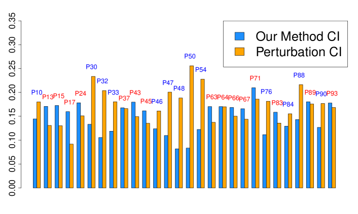
In the first step, we apply the adaptive Lasso procedure which selects 17 codons; in the second step, our method identifies additional 11 codons associated with drug resistance. Among 28 codons we identified, 13 of them are identified as strong signals and 15 of them as weak signals. Approach in [19] identified 18 codons, where the 13 signals (codon 10, 30, 32, 33, 46, 47, 48, 50, 54, 76, 84, 88 and 90) are the same as our strong-signal codons, and their remaining 5 signals (codon 37, 64, 71, 89 and 93) are among our 15 identified weak signals. In previous studies, [31] identifies all 13 strong signals using a permutation test for the regression coefficients obtained from Lasso; while [15] collect drug resistance mutation information based on multiple research studies, and discover 9 strong-signal codons (10, 32, 46, 47, 50, 54, 76, 84, 90) which are relevant to drug resistance. Neither of these approaches distinguish between strong-signal and weak-signal codons.

Figure 9 presents a graphical summary showing the half-width of the constructed confidence intervals based on our method and the perturbation approach, where strong signals are labeled in blue, and weak signals are labeled in red. To make full comparisons for both strong and weak signals, Figure 9 includes confidence intervals for all selected variables based on our method, even if some of them are not selected by approach in [19]. Table 5 also provides the average half-widths of confidence intervals in each signal category. In general, our method provides shorter lengths of confidence intervals for all strong signals, and longer lengths of confidence intervals for weak signals compared to the perturbation approach. This is not surprising, since the variables with weak coefficients associated with the response variable are relatively weaker, and likely result in wider confidence intervals to ensure a more accurate coverage. These findings are consistent with our simulation studies.

Figure 9: Half width of confidence intervals of selected signals for HIV data

Table 5: Average half width of the CIs

	All Selected Variables	Strong Signals	Weak Signals
$CI^{Our}$	0.147	0.118	0.173
$CI^{Ptb}$	0.171	0.197	0.148

In summary, our approach recovers more codons than other existing approaches. One significance of our method lies in its capability of identifying a pool of strong signals which have strong evidence association with HIV drug resistance, and a pool of possible weak signals which might be mildly associated with drug resistance. In many medical studies, it is important not to miss statistically weak signals, which could be clinically valuable predictors.

6 Summary and Discussion

In this paper, we propose weak signal identification under the penalized model selection framework, and develop a new two-step inferential method which is more accurate in providing confidence coverage for weak signal parameters in finite samples. The proposed method is applicable for true models involving both strong and weak signals. The primary concern regarding the existing model selection procedure is that it applies excessive shrinkage in order to achieve model selection consistency. However, this results in low detection power for weak signals in finite samples. The essence of the proposed method is to apply a mild tuning in identifying weak signals. Therefore, there is always a trade-off between a signal’s detection power and the false-discovery rate. In our approach, we intend to recover weak signals as much as possible, without sacrificing too much model selection consistency by including too many noise variables.

The two-step inference procedure imposes different selection criteria and confidence interval construction for strong and weak signals. Both theory and numerical studies indicate that the combined approach is more effective compared to the asymptotic inference approach, and bootstrap sampling and other resampling methods. In our numerical studies, we notice that the resampling methods do not provide good inference for weak signals. Specifically, the coverage probability of bootstrap confidence interval is over-covered and exceeds the $(1-\alpha)100\%$ confidence level when the true parameter is close to 0. This is not surprising, as [1] shows that the bootstrap procedure is inconsistent for boundary problems, such as in our case where the boundary parameters are in the order of $1/\sqrt{n}$.

Our method is related to post-selection inference in that we select variables if the corresponding estimated coefficients are not shrunk to zero, and then construct confidence intervals for those non-zero coefficients. This is quite different from the hypothesis testing approach which constructs valid confidence intervals for all variables first, then selects variables based on $p$-values or confidence intervals. One important work among the hypothesis testing approaches is the de-biased Lasso approach ([13]), which corrects the bias introduced by the Lasso procedure. The de-biased approach constructs valid confidence intervals and $p$-values for all variables, which is quite powerful when $p>n$ or the gram matrix is singular. However, this approach selects variables through the $p$-value. In contrast, we select variables if the corresponding estimated coefficients are not shrunk to zero, and construct confidence intervals for those non-zero coefficients. These two approaches are fundamentally different since some coefficients might not be statistically significant; however, the corresponding variables can still contribute to model prediction and should be included in the model. This difference is also reflected in our simulation studies in that the de-biased method has much lower detection rates for true signals in general, and especially when the signals are relatively weak.

In the proposed two-step inference procedure, although we utilize information from the least-square estimators, our approach is very different from applying the least-square inference directly without a model selection step. The non-penalization method is not feasible when the dimension of covariates is very large, e.g., to examine or visualize thousands of conference intervals without model selection. Therefore it is essential to make a sound statistical inference in conjunction with the variable selection, simultaneously. Our approach has several advantages: (1) It is able to recover possible weak signals which are missed due to excessive shrinkage in model selection, in addition to distinguishing weak signals from strong signals. (2) Our inferences are constructed for selected variable coefficients only. We eliminate noise variables first, and this is different from [19], [13], [27], and [33], which construct CIs for all variables. Consequently, the CI widths we construct for strong signals are much narrower compared to the least squared approach or de-biased method, given that the coverage rates are all accurate. This indicates that our procedure is more effective compared to the approaches which do not perform model selection first. This finding is not surprising since the full model including all the noise variables likely leads to less efficient inference in general. (3) For the weak signal CI’s, our numerical studies show that the proposed two-step approach provides CIs comparable to the least square’s, but has a much better coverage rate compared to the asymptotic, perturbation and resampling approaches.

In this paper, we develop our method and theory under the orthogonal design assumption. However, our numerical studies indicate that the proposed method is still valid when correlations among covariates are weak or moderate. It would be interesting to extend the current method to non-orthogonal designed covariates problems.

In addition, it is important to explore weak-signal inference for high-dimensional model settings when the dimension of covariates exceeds the sample size. Note that when the dimension of covariates exceeds the sample size, the least square estimator is no longer feasible, and cannot be used as the initial weights for the adaptive Lasso. One possible solution is to replace the full model $\hat{\theta}_{LS}$ by the marginal regression estimator. In order to do this, we assume that the true model satisfies the partial orthogonality condition, such that the covariates with zero coefficients and those with nonzero coefficients are weakly correlated, and the non-zero coefficients are bounded away from zero at certain rates. Under these assumptions, the estimator of the marginal regression coefficient satisfies the following property, such that the corresponding estimator is not too large for the zero coefficient, and not too small for the nonzero coefficient ([10]). This allows us to obtain a reasonable estimator to assign weights in the adaptive Lasso. The same idea has been adopted in [10], where marginal regression estimators are used to assign weights in the adaptive Lasso for sparse high-dimensional data. [10] and [11] show that the adaptive Lasso using the marginal estimator as initial weights yields model selection consistency under the partial orthogonality condition. Alternatively, we can first reduce the model size using the marginal screening approach ([7] and [18]), and then apply our method to the reduced size model. The marginal screening method ensures that we can reduce the model size to be smaller than the sample size, and thus the least square estimator $\hat{\theta}_{LS}$ can be obtained from a much smaller model.

Finally, the variance estimation of the penalized estimator for weak signal is still very challenging, and worthy of future research. In the proposed method, we use the least-square estimator to provide inference for weak signals. However, the variance of the least-square estimator $\hat{\sigma}_{LS}$ is inflated when $p$ is close to $n$. This is likely due to the gram matrix being close to singular when $p$ gets close to $n$ for the least-square estimation. We believe that the de-biased method ([13], [27]) could be very useful when the gram matrix is singular or close to singular, and it would be interesting to explore a future direction approximating a singular gram matrix to obtain parameter estimation and variance estimation as good as the de-biased method, and therefore to improve the precision of the confidence intervals for the proposed method.

Appendix A Notations and Proofs

A.1 Notations

$\nu_{0}=\sqrt{\lambda},\nu_{1}=z_{\tau/2}\frac{\sigma}{\sqrt{n}},\nu_{2}=\sqrt{\lambda}+z_{\alpha/2}\frac{\sigma}{\sqrt{n}},$ $\nu_{3}=(z_{\alpha/2}+z_{\tau/2})\frac{\sigma}{\sqrt{n}},$ $\nu_{4}=\sqrt{\lambda}+2z_{\alpha/2}\frac{\sigma}{\sqrt{n}}.$

A.2 Tuning Parameter Selection

BIC criteria function is:

$$BIC(\lambda)=log(\hat{\sigma}_{\lambda}^{2})+\hat{q}_{\lambda}\frac{log(n)}{n},$$

where $\hat{\sigma}_{\lambda}$ is the estimated standard deviation based on $\lambda$, and $\hat{q}_{\lambda}$ is the number of covariates in the model.

We choose the tuning parameter $\lambda$ based on the BIC because of its consistency property to select the true model ([30]). Here we follow the strategy in [28] to select the BIC tuning parameter for the adaptive Lasso penalty. Specifically, for a given $\lambda$,

$$BIC(\lambda)=(\bm{\widehat{\theta}}_{\lambda}-\bm{\widehat{\theta}}_{LS})^{T}\bm{\widehat{\Sigma}}^{-1}_{\lambda}(\bm{\widehat{\theta}}_{\lambda}-\bm{\widehat{\theta}}_{LS})+\hat{q}_{\lambda}log(n)/n,$$

where $\bm{\widehat{\theta}}_{\lambda}$ is the adaptive Lasso estimator with a tuning parameter $\lambda$ provided in (2.1); $\bm{\widehat{\Sigma}}^{-1}_{\lambda}=(n\hat{\sigma}^{2})^{-1}\left\{\bm{X}^{T}\bm{X}+n\lambda\mbox{diag}\{I(\hat{\theta}_{\lambda,j}\neq 0)/|\hat{\theta}_{\lambda,j}\hat{\theta}_{LS,j}|\}_{j=1}^{p}\right\}$; $\hat{\sigma}$ is a consistent estimator of $\sigma$ based on the scaled Lasso procedure ([25]); and $\hat{q}_{\lambda}$ is the number of nonzero coefficients of $\bm{\widehat{\theta}}_{\lambda}$, a simple estimator for the degree of freedom ([35]).

A.3 Proof of Lemma 1

Proof.

For any $\gamma$ satisfies $\epsilon<\gamma<1-\epsilon$, we show that $\nu^{\gamma}$ that solves $P_{d}=\gamma$ follows $\frac{\nu^{\gamma}}{\sqrt{\lambda_{n}}}\rightarrow 1$, as $n\rightarrow\infty$.

$P_{d}$ can be rewritten as $P_{d}=\Phi(\frac{\sqrt{n\lambda_{n}}}{\sigma}(\frac{\nu^{\gamma}}{\sqrt{\lambda_{n}}}-1))-\Phi(-\frac{\sqrt{n\lambda_{n}}}{\sigma}(1+\frac{\nu^{\gamma}}{\sqrt{\lambda_{n}}}))$. Given $n\lambda_{n}\rightarrow\infty$, if $\lim_{n\to+\infty}\frac{\nu^{\gamma}}{\sqrt{\lambda_{n}}}>1,$ then $P_{d}(\nu^{\gamma})\rightarrow 1$, as $n\rightarrow\infty$; else if $\lim_{n\to+\infty}\frac{\nu^{\gamma}}{\sqrt{\lambda_{n}}}<1,$ then $P_{d}(\nu^{\gamma})\rightarrow 0,$ as $n\rightarrow\infty.$ Since $P_{d}(\nu^{\gamma})=\gamma\in\left(\epsilon,1-\epsilon\right),$ we have $\lim_{n\to+\infty}\frac{\nu^{\gamma}}{\sqrt{\lambda_{n}}}=1,$ as $n\rightarrow\infty.$

Therefore, both $\nu^{s}$ and $\nu^{w}$ satisfies $\frac{\nu^{s}}{\sqrt{\lambda_{n}}}\rightarrow 1$ and $\frac{\nu^{w}}{\sqrt{\lambda_{n}}}\rightarrow 1$. ∎

A.4 Proof of Lemma 2

Proof.

Define $CI_{a}:\left\{\theta:|\hat{\theta}_{LS}-\theta|<z_{\alpha/2}\tilde{\sigma}(\theta)/\sqrt{n}\right\}$, and $CI_{b}:\left\{\theta:|\hat{\theta}_{LS}-\theta|<z_{\alpha/2}\sigma/\sqrt{n}\right\}$. The confidence interval in (4.1) can be rewritten as:

$$CI_{a}\cdot I_{\left\{|\hat{\theta}_{LS}|\geq\nu_{2}\right\}}+CI_{b}\cdot I_{\left\{\nu_{1}<|\hat{\theta}_{LS}|<\nu_{2}\right\}}.$$

Based on $CI_{a},CI_{b}$, we define functions $CR_{a}(\theta,\nu),CR_{b}(\theta,\nu)$ in the following manners:

$$CR_{a}(\theta,\nu)=P(\theta\in CI_{a},|\hat{\theta}_{LS}|>\nu),$$ (A.1)

$$CR_{b}(\theta,\nu)=P(\theta\in CI_{b},|\hat{\theta}_{LS}|>\nu){\sigma/\sqrt{n}}).$$ (A.2)

Besides, define $P_{s}(\theta,\nu)$ as $P(|\hat{\theta}_{LS}|>\nu)$, which equals to

$$P_{s}(\theta,\nu)=\Phi(\frac{\theta-\nu}{\sigma/\sqrt{n}})+\Phi(\frac{-\theta-\nu}{\sigma/\sqrt{n}}).$$ (A.3)

The explicit expression of $CR_{a}(\theta,\nu)$ is derived based on three cases:
(i). If $\nu<\theta-z_{\alpha/2}\frac{\tilde{\sigma}(\theta)}{\sqrt{n}}$, then

$$CR_{a}(\theta,\nu)=P\left(|\hat{\theta}^{LS}-\theta|\leq z_{\alpha/2}\frac{\tilde{\sigma}(\theta)}{\sqrt{n}}\right)=1-2\Phi(-z_{\alpha/2}\frac{\tilde{\sigma}(\theta)}{\sigma}).$$

(ii). If $|\theta-z_{\alpha/2}\frac{\tilde{\sigma}(\theta)}{\sqrt{n}}|<\nu<\theta+z_{\alpha/2}\frac{\tilde{\sigma}(\theta)}{\sqrt{n}}$, then

$$CR_{a}(\theta,\nu)=P\left(\nu<\hat{\theta}^{LS}<\theta+z_{\alpha/2}\frac{\tilde{\sigma}(\theta)}{\sqrt{n}}\right)=\Phi(z_{\alpha/2}\frac{\tilde{\sigma}(\theta)}{\sigma})-\Phi(\frac{\nu-\theta}{\sigma/\sqrt{n}}).$$

(iii). If $\nu<-\theta+z_{\alpha/2}\frac{\tilde{\sigma}(\theta)}{\sqrt{n}}$, then

$$CR_{a}(\theta,\nu) = P\left(\theta-z_{\alpha/2}\frac{\tilde{\sigma}(\theta)}{\sqrt{n}}<\hat{\theta}^{LS}<-\nu\right)+P\left(\nu<\hat{\theta}^{LS}<\theta+z_{\alpha/2}\frac{\tilde{\sigma}(\theta)}{\sqrt{n}}\right)$$

$$= P_{s}(\theta,\nu)-2\Phi(-z_{\alpha/2}\frac{\tilde{\sigma}(\theta)}{\sigma}).$$

The expression of $CR_{b}(\theta,\nu)$ can be derived in a similar way. Therefore, $CR_{a}(\theta,\nu)$ and $CR_{b}(\theta,\nu)$ have the explicit expressions as:

$$CR_{a}(\theta,\nu)=\begin{cases}\left(P_{s}(\theta,\nu)-2\Phi(-z_{\alpha/2}\frac{\tilde{\sigma}(\theta)}{\sigma})\right)\cdot\\ I_{\left\{\nu<z_{\alpha/2}\frac{\tilde{\sigma}(\theta)}{\sqrt{n}}\right\}}&\mbox{if }|\theta|<|\nu-z_{\alpha/2}\frac{\tilde{\sigma}(\theta)}{\sqrt{n}}|,\\ \Phi(z_{\alpha/2}\frac{\tilde{\sigma}(\theta)}{\sigma})-\Phi(\frac{\nu-\theta}{\sigma/\sqrt{n}})&\mbox{if }|\nu-z_{\alpha/2}\frac{\tilde{\sigma}(\theta)}{\sqrt{n}}|\leq|\theta|\leq\nu+z_{\alpha/2}\frac{\tilde{\sigma}(\theta)}{\sqrt{n}},\\ 1-2\Phi(-z_{\alpha/2}\frac{\tilde{\sigma}(\theta)}{\sigma})&\mbox{if }|\theta|>\nu+z_{\alpha/2}\frac{\tilde{\sigma}(\theta)}{\sqrt{n}},\end{cases}$$

and

$$CR_{b}(\theta,\nu)=\begin{cases}\left(P_{s}(\theta,\nu)-\alpha\right)1_{\left\{\nu<z_{\alpha/2}\frac{\sigma}{\sqrt{n}}\right\}}&\mbox{if }|\theta|<|\nu-z_{\alpha/2}\frac{\sigma}{\sqrt{n}}|,\\ 1-\frac{\alpha}{2}-\Phi(\frac{\nu-\theta}{\sigma/\sqrt{n}})&\mbox{if }|\nu-z_{\alpha/2}\frac{\sigma}{\sqrt{n}}|<|\theta|<\nu+z_{\alpha/2}\frac{\sigma}{\sqrt{n}},\\ 1-\alpha&\mbox{if }|\theta|>\nu+z_{\alpha/2}\frac{\sigma}{\sqrt{n}}.\end{cases}$$

The equations in (A.1)-(A.3) are used to provide explicit expressions for $CR_{1}(\theta)$ and $CR(\theta)$ in Lemma 2. More specifically,

$$CR_{1}(\theta) = P(\theta\mbox{ in asymptotic-based CI}|\theta\mbox{ is selected in model selection})$$

$$= \left.P(|\hat{\theta}_{LS}-\theta|<z_{\alpha/2}\frac{\tilde{\sigma}(\theta)}{\sqrt{n}}\right||\hat{\theta}_{LS}|>\sqrt{\lambda})$$

$$= \frac{CR_{a}(\theta,\nu_{0})}{P_{s}(\theta,\nu_{0})},$$

where $\nu_{0}=\sqrt{\lambda}$. Similarly,

$$CR(\theta) = P(\theta\in\mbox{ CI as in (\ref{inf}) }|\theta\mbox{ is selected by the two-step procedure})$$

$$= \frac{P(\theta\in CI_{a},|\hat{\theta}_{LS}|\geq\nu_{2})+P(\theta\in CI_{b},\nu_{1}<|\hat{\theta}_{LS}|<\nu_{2})}{P(|\hat{\theta}_{LS}|>\nu_{1})}$$

$$= \frac{P(\theta\in CI_{a},|\hat{\theta}_{LS}|\geq\nu_{2})+P(\theta\in CI_{b},|\hat{\theta}_{LS}|>\nu_{2})-P(\theta\in CI_{b},|\hat{\theta}_{LS}|>\nu_{1})}{P(|\hat{\theta}_{LS}|>\nu_{1})}$$

$$= \frac{CR_{a}(\theta,\nu_{2})+CR_{b}(\theta,\nu_{1})-CR_{b}(\theta,\nu_{2})}{P_{s}(\theta,\nu_{1})}.$$

∎

A.5 Lemmas

Lemma 3.

If we select $\nu_{1}=z_{\tau/2}\frac{\sigma}{\sqrt{n}}$, then the false positive rate of weak signal’s identification procedure equals $\tau$.

Proof.

By definition, the false positive rate equals $P(i\in\widehat{\bm{S}}^{\bm{(W)}}\cup\bm{\widehat{S}^{(S)}}|\theta_{i}=0)=P(|\hat{\theta}_{LS,i}|>\nu_{1}|\theta_{i}=0)=2\Phi(-\frac{\sqrt{n}}{\sigma}\nu_{1})=\tau.$ ∎

Lemma 4.

Under conditions (C1)-(C2), when $\lambda$ satisfies conditions $\sqrt{\lambda}>z_{\alpha/2}\frac{\sigma}{\sqrt{n}}$,

1. if $c_{1}$ is the solution to $\theta=\sqrt{\lambda}-z_{\alpha/2}\frac{\tilde{\sigma}(\theta)}{\sqrt{n}}$, then $c_{1}\in\left((z_{\alpha/2}-z_{\tau/2})\frac{\sigma}{\sqrt{n}},\sqrt{\lambda}\right);$

2. if $c_{2}$ is the solution to $\theta=\sqrt{\lambda}+z_{\alpha/2}\frac{\tilde{\sigma}(\theta)}{\sqrt{n}}$, then $c_{2}\in\left(\sqrt{\lambda}+\frac{1}{2}z_{\alpha/2}\frac{\sigma}{\sqrt{n}},\sqrt{\lambda}+z_{\alpha/2}\frac{\sigma}{\sqrt{n}}\right);$

3. if $c_{3}$ is the solution to $\theta=\sqrt{\lambda}+z_{\alpha/2}\frac{\sigma}{\sqrt{n}}-z_{\alpha/2}\frac{\tilde{\sigma}(\theta)}{\sqrt{n}}$, then $c_{3}\in\left(\sqrt{\lambda},\sqrt{\lambda}+\frac{1}{2}z_{\alpha/2}\frac{\sigma}{\sqrt{n}}\right);$

4. if $c_{4}$ is the solution to $\theta=\sqrt{\lambda}+z_{\alpha/2}\frac{\sigma}{\sqrt{n}}+z_{\alpha/2}\frac{\tilde{\sigma}(\theta)}{\sqrt{n}}$, then
   $c_{4}\in\left(\sqrt{\lambda}+\frac{3}{2}z_{\alpha/2}\frac{\sigma}{\sqrt{n}},\sqrt{\lambda}+2z_{\alpha/2}\frac{\sigma}{\sqrt{n}}\right).$

In addition, the order relationships of $c_{1},c_{2},c_{3}$ and $c_{4}$ follow: $c_{1}<c_{3}<c_{2}<c_{4}.$

Lemma 5.

Given $\theta\in\left(\sqrt{\lambda}+\frac{1}{2}z_{\alpha/2}\frac{\sigma}{\sqrt{n}},\sqrt{\lambda}+2z_{\alpha/2}\frac{\sigma}{\sqrt{n}}\right)$, then $\theta>c_{2}$ if and only if $\theta>\sqrt{\lambda}+z_{\alpha/2}\frac{\tilde{\sigma}(\theta)}{\sqrt{n}}$, and $\theta>c_{4}$ if and only if $\theta>\sqrt{\lambda}+z_{\alpha/2}\frac{\sigma}{\sqrt{n}}+z_{\alpha/2}\frac{\tilde{\sigma}(\theta)}{\sqrt{n}}$.

Lemma 6.

(Monotonicity of $CR_{1}(\theta)$)
Suppose $\theta>0,$ $CR_{1}(\theta)$ is a piece-wise monotonic function on $\left[0,c_{2}\right]$. More specifically, $CR_{1}(\theta)$ is a non-decreasing function on $\left[0,c_{1}\right]$, an increasing function on $\left[c_{1},c_{2}\right]$.

Lemma 7.

For any fixed parameter value $\nu>0$, the function

$$\frac{CR_{b}(\theta,\nu)}{P_{s}(\theta,\nu)}=\begin{cases}\left(1-\frac{\alpha}{P_{s}(\theta,\nu)}\right)1_{\left\{\nu<z_{\alpha/2}\frac{\sigma}{\sqrt{n}}\right\}}&\mbox{if }|\theta|<|\nu-z_{\alpha/2}\frac{\sigma}{\sqrt{n}}|\\ \frac{1-\frac{\alpha}{2}-\Phi\left(\frac{\sqrt{n}}{\sigma}(\nu-\theta)\right)}{P_{s}(\theta,\nu)}&\mbox{if }|\nu-z_{\alpha/2}\frac{\sigma}{\sqrt{n}}|<|\theta|<\nu+z_{\alpha/2}\frac{\sigma}{\sqrt{n}}\\ \frac{1-\alpha}{P_{s}(\theta,\nu)}&\mbox{if }|\theta|>\nu+z_{\alpha/2}\frac{\sigma}{\sqrt{n}},\end{cases}$$

is

1. non-decreasing, when $|\theta|\leq|\nu-z_{\alpha/2}\frac{\sigma}{\sqrt{n}}|;$

2. increasing, when $|\nu-z_{\alpha/2}\frac{\sigma}{\sqrt{n}}|<|\theta|<\nu+z_{\alpha/2}\frac{\sigma}{\sqrt{n}};$

3. decreasing, when $|\theta|\geq\nu+z_{\alpha/2}\frac{\sigma}{\sqrt{n}}.$

Lemma 8.

The formulas for $CR_{1}(\theta)$ and $CR(\theta)$ in Lemma 2 can also be expressed as:

$$CR_{1}(\theta) = \frac{CR_{a}(\theta,\nu_{0})}{P_{s}(\theta,\nu_{0})},$$ (A.4)

$$CR(\theta) = \begin{cases}\frac{CR_{b}(\theta,\nu_{1})}{P_{s}(\theta,\nu_{1})}&\mbox{if }|\theta|<\nu_{0}\\ \frac{CR_{b}(\theta,\nu_{1})}{P_{s}(\theta,\nu_{1})}-\frac{CR_{b}(\theta,\nu_{2})}{P_{s}(\theta,\nu_{1})}&\mbox{if }\nu_{0}\leq|\theta|\leq c_{3}\\ \frac{CR_{b}(\theta,\nu_{1})}{P_{s}(\theta,\nu_{1})}+\frac{CR_{a}(\theta,\nu_{2})}{P_{s}(\theta,\nu_{1})}-\frac{CR_{b}(\theta,\nu_{2})}{P_{s}(\theta,\nu_{1})}&\mbox{if }|\theta|>c_{3}.\end{cases}$$ (A.5)

Then $CR_{1}(\theta)=J_{1}(\theta),CR(\theta)=J_{2}(\theta)-J_{3}(\theta)+J_{4}(\theta)$, where the four functions $J_{1}(\theta),J_{2}(\theta),J_{3}(\theta)$ and $J_{4}(\theta)$ are defined as:

$$J_{1}(\theta)=\frac{CR_{a}(\theta,\nu_{0})}{P_{s}(\theta,\nu_{0})},J_{2}(\theta)=\frac{CR_{b}(\theta,\nu_{1})}{P_{s}(\theta,\nu_{1})},$$

$$J_{3}(\theta)=\frac{CR_{b}(\theta,\nu_{2})}{P_{s}(\theta,\nu_{1})},J_{4}(\theta)=\frac{CR_{a}(\theta,\nu_{2})}{P_{s}(\theta,\nu_{1})}.$$

A.6 Proof of Theorem 1

Proof.

(a). When $\theta\in\left[0,c_{1}\right]$, we have $\Delta(\theta)\geq 1-\frac{\alpha}{\tau}>0.$ First, it is obvious that $CR_{1}(\theta)=0$ when $\theta\in\left[0,c_{1}\right]$. By Lemma 7, $CR(\theta)$ is increasing on $\left[0,\nu_{0}\right]$, and $CR(\theta)=1-\frac{\alpha}{\tau}$ when $\theta=0$. Thus $CR(\theta)-CR_{1}(\theta)\geq 1-\frac{\alpha}{\tau}$ for $\theta\in\left[0,c_{1}\right]$, which provides the first lower bound in Theorem 1. Note that here we also use $c_{1}<\nu_{0}$ by Lemma 4.

(b). When $\theta\in\left[c_{1},\nu_{0}\right],$ we have $\Delta(\theta)\geq\frac{2}{1+\alpha}-2\Phi(\frac{1}{2}z_{\alpha/2})>0$. By definition

$$CR_{1}(\theta) = \frac{\Phi\left(z_{\alpha/2}\frac{\tilde{\sigma}(\theta)}{\sigma}\right)-\Phi\left(\frac{\sqrt{n}}{\sigma}(\nu_{0}-\theta)\right)}{P_{s}(\theta,\nu_{0})},$$

$$CR(\theta) = \frac{1-\frac{\alpha}{2}-\Phi\left(\frac{\sqrt{n}}{\sigma}(\nu_{1}-\theta)\right)}{P_{s}(\theta,\nu_{1})}.$$

In the following, we show that $\frac{\partial{CR_{1}(\theta)}}{\partial{\theta}}>\frac{\partial{CR(\theta)}}{\partial{\theta}}$, so $CR(\theta)-CR_{1}(\theta)$ is decreasing when $\theta\in\left[c_{1},\nu_{0}\right]$. The first order derivatives of $CR_{1}(\theta)$ and $CR(\theta)$ are:

$$\frac{\partial{CR_{1}(\theta)}}{\partial{\theta}} = \left[\frac{z_{\alpha/2}}{\sigma}\phi\left(z_{\alpha/2}\frac{\tilde{\sigma}(\theta)}{\sigma}\right)\tilde{\sigma}(\theta)^{\prime}+\frac{\sqrt{n}}{\sigma}\phi\left(\frac{\sqrt{n}}{\sigma}(\nu_{0}-\theta)\right)\right]P_{s}(\theta,\nu_{0})^{-1}$$ (A.7)

$$-\left[\Phi\left(z_{\alpha/2}\frac{\tilde{\sigma}(\theta)}{\sigma}\right)-\Phi\left(\frac{\sqrt{n}}{\sigma}(\nu_{0}-\theta)\right)\right]P_{s}(\theta,\nu_{0})^{-2}$$

$$\frac{\partial{CR(\theta)}}{\partial{\theta}} = \frac{\sqrt{n}}{\sigma}\phi\left(\frac{\sqrt{n}}{\sigma}(\nu_{1}-\theta)\right)P_{s}(\theta,\nu_{1})^{-1}$$ (A.9)

$$-\left[1-\frac{\alpha}{2}-\Phi\left(\frac{\sqrt{n}}{\sigma}(\nu_{1}-\theta)\right)\right]P_{s}(\theta,\nu_{1})^{-2},$$

where each first-order derivative is composed of two parts. We show the inequality of each part separately. First (A.7) $>$ (A.9), which is sufficient by showing

$$\phi\left(\frac{\sqrt{n}}{\sigma}(\nu_{0}-\theta)\right)P_{s}(\theta,\nu_{0})^{-1}>\phi\left(\frac{\sqrt{n}}{\sigma}(\nu_{1}-\theta)\right)P_{s}(\theta,\nu_{1})^{-1}.$$

This is equivalent to show

$$\frac{\Phi\left(\frac{\sqrt{n}}{\sigma}(\theta-\nu_{1})\right)+\Phi\left(-\frac{\sqrt{n}}{\sigma}(\theta+\nu_{1})\right)}{\phi\left(\frac{\sqrt{n}}{\sigma}(\theta-\nu_{1})\right)}>\frac{\Phi\left(\frac{\sqrt{n}}{\sigma}(\theta-\nu_{0})\right)+\Phi\left(-\frac{\sqrt{n}}{\sigma}(\theta+\nu_{0})\right)}{\phi\left(\frac{\sqrt{n}}{\sigma}(\theta-\nu_{0})\right)}.$$ (A.10)

The inequality in (A.10) can be proved based on monotinicity of two functions $\frac{\Phi(x)}{\phi(x)}$ and $\frac{\Phi(-x-y)}{\phi(x-y)}$. Specifically, it can be shown that $\frac{\Phi(x)}{\phi(x)}$ is an increasing function of $x\in\mathbbm{R}$, and $\frac{\Phi(-x-y)}{\phi(x-y)}$ is a decreasing function of $y\in\mathbbm{R^{+}}$, for any fixed value of $x>0$. More specifically, since $\nu_{1}<\nu_{0},$ we have

$$\frac{\Phi\left(\frac{\sqrt{n}}{\sigma}(\theta-\nu_{1})\right)}{\phi\left(\frac{\sqrt{n}}{\sigma}(\theta-\nu_{1})\right)}>\frac{\Phi\left(\frac{\sqrt{n}}{\sigma}(\theta-\nu_{0})\right)}{\phi\left(\frac{\sqrt{n}}{\sigma}(\theta-\nu_{0})\right)}\mbox{ and }\frac{\Phi\left(-\frac{\sqrt{n}}{\sigma}(\theta+\nu_{1})\right)}{\phi\left(\frac{\sqrt{n}}{\sigma}(\theta-\nu_{1})\right)}>\frac{\Phi\left(-\frac{\sqrt{n}}{\sigma}(\theta+\nu_{0})\right)}{\phi\left(\frac{\sqrt{n}}{\sigma}(\theta-\nu_{0})\right)},$$

based on which the inequality in (A.10) holds.

Next we show that (A.9) $<$ (A.9), which is equivalent with

$$\left[1-\frac{\alpha}{2}-\Phi\left(\frac{\sqrt{n}}{\sigma}(\nu_{1}-\theta)\right)\right]P_{s}(\theta,\nu_{1})^{-2}>\left[\Phi\left(z_{\alpha/2}\frac{\tilde{\sigma}(\theta)}{\sigma}\right)-\Phi\left(\frac{\sqrt{n}}{\sigma}(\nu_{1}-\theta)\right)\right]P_{s}(\theta,\nu_{0})^{-2}.$$

It can be shown by

$$\frac{1-\frac{\alpha}{2}-\Phi\left(\frac{\sqrt{n}}{\sigma}(\nu_{1}-\theta)\right)}{{P_{s}(\theta,\nu_{1})}^{2}}>\frac{1-\frac{\alpha}{2}-\Phi\left(\frac{\sqrt{n}}{\sigma}(\nu_{0}-\theta)\right)}{{P_{s}(\theta,\nu_{0})}^{2}}>\frac{\Phi\left(z_{\alpha/2}\frac{\tilde{\sigma}(\theta)}{\sigma}\right)-\Phi\left(\frac{\sqrt{n}}{\sigma}(\nu_{1}-\theta)\right)}{{P_{s}(\theta,\nu_{0})}^{2}}.$$

Based on the above arguments, we can conclude that for $\theta\in\left[c_{1},\nu_{0}\right]$:

$$\frac{\partial{CR_{1}(\theta)}}{\partial{\theta}}>\frac{\partial{CR(\theta)}}{\partial{\theta}}.$$

Therefore, $\min_{\theta\in\left[c_{1},\nu_{0}\right]}\Delta(\theta)=CR(\nu_{0})-CR_{1}(\nu_{0}).$ More specifically,

$$CR(\nu_{0}) = \frac{\Phi(\frac{\nu_{0}-\nu_{1}}{\sigma/\sqrt{n}})-\frac{\alpha}{2}}{\Phi(\frac{\nu_{0}-\nu_{1}}{\sigma/\sqrt{n}})+\Phi(\frac{-\nu_{0}-\nu_{1}}{\sigma/\sqrt{n}})}>\frac{1-\alpha}{1+\alpha},$$

$$CR_{1}(\nu_{0}) = \frac{\Phi(\frac{1}{2}z_{\alpha/2})-\frac{\alpha}{2}}{\frac{1}{2}+\Phi(-\frac{2\nu_{0}}{\sigma/\sqrt{n}})}<2\Phi(\frac{1}{2}z_{\alpha/2})-1,$$

thus

$$CR(\nu_{0}) - CR_{1}(\nu_{0})>\frac{2}{1+\alpha}-2\Phi(\frac{1}{2}z_{\alpha/2}),$$

which provides the second lower bound in Theorem 1.

(c). When $\theta\in\left[\nu_{0},+\infty\right),$ we have $\Delta(\theta)$ satisfies either $\Delta(\theta)\geq 0$ or $-\frac{\alpha}{2}<\Delta(\theta)<0$. The proof of case 1 is provided here, and proof of the other two cases are similar and are provided in supplementary materials. In case 1, it satisfies $c_{3}<\nu_{3}<c_{2}$. We conduct derivations for sub-intervals $\left[\nu_{0},c_{3}\right],\left[c_{3},\nu_{3}\right],\left[\nu_{3},c_{2}\right],\left[c_{2},c_{4}\right],\left[c_{4},\nu_{4}\right]$ and $\left[\nu_{4},+\infty\right)$, separately.

When $\theta\in\left[\nu_{0},c_{3}\right]$, we have

$$J_{1}(\theta) = \frac{\Phi(z_{\alpha/2}\frac{\tilde{\sigma}(\theta)}{\sigma})-\Phi(\frac{\nu_{0}-\theta}{\sigma/\sqrt{n}})}{\Phi(\frac{\theta-\nu_{0}}{\sigma/\sqrt{n}})+\Phi(\frac{-\theta-\nu_{0}}{\sigma/\sqrt{n}})},J_{2}(\theta)=\frac{1-\frac{\alpha}{2}-\Phi(\frac{\nu_{1}-\theta}{\sigma/\sqrt{n}})}{\Phi(\frac{\theta-\nu_{1}}{\sigma/\sqrt{n}})+\Phi(\frac{-\theta-\nu_{1}}{\sigma/\sqrt{n}})},$$

$$\mbox{ and }J_{3}(\theta) = \frac{1-\frac{\alpha}{2}-\Phi(\frac{\nu_{2}-\theta}{\sigma/\sqrt{n}})}{\Phi(\frac{\theta-\nu_{1}}{\sigma/\sqrt{n}})+\Phi(\frac{-\theta-\nu_{1}}{\sigma/\sqrt{n}})},$$

thus

$$\Delta(\theta) = J_{2}(\theta)-J_{1}(\theta)-J_{3}(\theta)$$

$$= \frac{\Phi(\frac{\nu_{2}-\theta}{\sigma/\sqrt{n}})-\Phi(\frac{\nu_{1}-\theta}{\sigma/\sqrt{n}})}{\Phi(\frac{\theta-\nu_{1}}{\sigma/\sqrt{n}})+\Phi(\frac{-\theta-\nu_{1}}{\sigma/\sqrt{n}})}-\frac{\Phi(z_{\alpha/2}\frac{\tilde{\sigma}(\theta)}{\sigma})-\Phi(\frac{\nu_{0}-\theta}{\sigma/\sqrt{n}})}{\Phi(\frac{\theta-\nu_{0}}{\sigma/\sqrt{n}})+\Phi(\frac{-\theta-\nu_{0}}{\sigma/\sqrt{n}})}.$$

Further,

$$\Delta(\theta) = \frac{\Phi(\frac{\nu_{2}-\theta}{\sigma/\sqrt{n}})-\Phi(\frac{\nu_{1}-\theta}{\sigma/\sqrt{n}})}{\Phi(\frac{\theta-\nu_{1}}{\sigma/\sqrt{n}})+\Phi(\frac{-\theta-\nu_{1}}{\sigma/\sqrt{n}})}-\frac{\Phi(z_{\alpha/2}\frac{\tilde{\sigma}(\theta)}{\sigma})-\Phi(\frac{\nu_{0}-\theta}{\sigma/\sqrt{n}})}{\Phi(\frac{\theta-\nu_{0}}{\sigma/\sqrt{n}})+\Phi(\frac{-\theta-\nu_{0}}{\sigma/\sqrt{n}})}$$

$$> \frac{\Phi(\frac{\nu_{2}-\theta}{\sigma/\sqrt{n}})-\Phi(\frac{\nu_{1}-\theta}{\sigma/\sqrt{n}})}{\Phi(\frac{\theta-\nu_{1}}{\sigma/\sqrt{n}})+\Phi(\frac{-\theta-\nu_{1}}{\sigma/\sqrt{n}})}-\frac{\Phi(z_{\alpha/2}\frac{\tilde{\sigma}(\theta)}{\sigma})-\Phi(\frac{\nu_{0}-\theta}{\sigma/\sqrt{n}})}{\Phi(\frac{\theta-\nu_{0}}{\sigma/\sqrt{n}})}$$

$$> \frac{\Phi(\frac{\nu_{2}-\theta}{\sigma/\sqrt{n}})-\Phi(\frac{\nu_{1}-\theta}{\sigma/\sqrt{n}})}{\Phi(\frac{\theta-\nu_{1}}{\sigma/\sqrt{n}})+\Phi(\frac{-\theta-\nu_{1}}{\sigma/\sqrt{n}})}-\frac{\Phi(\frac{\nu_{2}-\theta}{\sigma/\sqrt{n}})-\Phi(\frac{\nu_{0}-\theta}{\sigma/\sqrt{n}})}{\Phi(\frac{\theta-\nu_{0}}{\sigma/\sqrt{n}})}$$

$$= \frac{\left[\Phi(\frac{\nu_{2}-\theta}{\sigma/\sqrt{n}})-\Phi(\frac{\nu_{1}-\theta}{\sigma/\sqrt{n}})\right]\Phi(\frac{\theta-\nu_{0}}{\sigma/\sqrt{n}})-\left[\Phi(\frac{\nu_{2}-\theta}{\sigma/\sqrt{n}})-\Phi(\frac{\nu_{0}-\theta}{\sigma/\sqrt{n}})\right]\Phi(\frac{\theta-\nu_{1}}{\sigma/\sqrt{n}})}{\left[\Phi(\frac{\theta-\nu_{1}}{\sigma/\sqrt{n}})+\Phi(\frac{-\theta-\nu_{1}}{\sigma/\sqrt{n}})\right]\Phi(\frac{\theta-\nu_{0}}{\sigma/\sqrt{n}})}$$

$$-\frac{\left[\Phi(\frac{\nu_{2}-\theta}{\sigma/\sqrt{n}})-\Phi(\frac{\nu_{0}-\theta}{\sigma/\sqrt{n}})\right]\Phi(\frac{-\theta-\nu_{1}}{\sigma/\sqrt{n}})}{\left[\Phi(\frac{\theta-\nu_{1}}{\sigma/\sqrt{n}})+\Phi(\frac{-\theta-\nu_{1}}{\sigma/\sqrt{n}})\right]\Phi(\frac{\theta-\nu_{0}}{\sigma/\sqrt{n}})}$$

$$= \Delta_{1}(\theta)-\Delta_{2}(\theta),$$

where the second inequality uses that $z_{\alpha/2}\frac{\tilde{\sigma}(\theta)}{\sqrt{n}}\leq\nu_{2}-\theta$ when $\theta\leq c_{3}$ by Lemma 5. Here $\Delta_{1}(\theta)$ and $\Delta_{2}(\theta)$ are defined as:

$$\Delta_{1}(\theta) = \frac{\left[\Phi(\frac{\nu_{2}-\theta}{\sigma/\sqrt{n}})-\Phi(\frac{\nu_{1}-\theta}{\sigma/\sqrt{n}})\right]\Phi(\frac{\theta-\nu_{0}}{\sigma/\sqrt{n}})-\left[\Phi(\frac{\nu_{2}-\theta}{\sigma/\sqrt{n}})-\Phi(\frac{\nu_{0}-\theta}{\sigma/\sqrt{n}})\right]\Phi(\frac{\theta-\nu_{1}}{\sigma/\sqrt{n}})}{\left[\Phi(\frac{\theta-\nu_{1}}{\sigma/\sqrt{n}})+\Phi(\frac{-\theta-\nu_{1}}{\sigma/\sqrt{n}})\right]\Phi(\frac{\theta-\nu_{0}}{\sigma/\sqrt{n}})},$$

$$\Delta_{2}(\theta) = \frac{\left[\Phi(\frac{\nu_{2}-\theta}{\sigma/\sqrt{n}})-\Phi(\frac{\nu_{0}-\theta}{\sigma/\sqrt{n}})\right]}{\left[\Phi(\frac{\theta-\nu_{1}}{\sigma/\sqrt{n}})+\Phi(\frac{-\theta-\nu_{1}}{\sigma/\sqrt{n}})\right]\Phi(\frac{\theta-\nu_{0}}{\sigma/\sqrt{n}})}\Phi(\frac{-\theta-\nu_{1}}{\sigma/\sqrt{n}}).$$

First, it is straightforward to show that $\Delta_{1}(\theta)>0$. Second, $\Delta_{2}(\theta)$ can be bounded from above by some small value. In fact,

$$\Delta_{2}(\theta) < \frac{\left[\Phi(\frac{\nu_{2}-\theta}{\sigma/\sqrt{n}})-\Phi(\frac{\nu_{0}-\theta}{\sigma/\sqrt{n}})\right]}{\Phi(\frac{\theta-\nu_{1}}{\sigma/\sqrt{n}})\Phi(\frac{\theta-\nu_{0}}{\sigma/\sqrt{n}})}\Phi(\frac{-\theta-\nu_{1}}{\sigma/\sqrt{n}})$$

$$< 4\left[\Phi(\frac{\nu_{2}-\theta}{\sigma/\sqrt{n}})-\Phi(\frac{\nu_{0}-\theta}{\sigma/\sqrt{n}})\right]\Phi(\frac{-\theta-\nu_{1}}{\sigma/\sqrt{n}})$$

$$< 4\left[1-\frac{\alpha}{2}-\Phi(-\frac{1}{2}z_{\alpha/2})\right]\Phi(-\frac{3}{2}z_{\alpha/2}),$$

where we use that $\nu_{2}-\theta<z_{\alpha/2}\frac{\sigma}{\sqrt{n}}$, $-\frac{1}{2}z_{\alpha/2}\frac{\sigma}{\sqrt{n}}<\nu_{0}-c_{3}<\nu_{0}-\theta$ and $\Phi(\frac{-\theta-\nu_{1}}{\sigma/\sqrt{n}})<\Phi(\frac{-\nu_{0}-\nu_{1}}{\sigma/\sqrt{n}})<\Phi(-\frac{3}{2}z_{\alpha/2})$ when $\nu_{0}<\theta<c_{3}$. Combining the lower bounds for $\Delta_{1}(\theta)$ and $\Delta_{2}(\theta)$, we have:

$$\Delta(\theta)>-4\left[1-\frac{\alpha}{2}-\Phi(-\frac{1}{2}z_{\alpha/2})\right]\Phi(-\frac{3}{2}z_{\alpha/2}).$$

In fact, the lower bound on the right hand side is quite close to zero.

When $\theta\in\left[c_{3},\nu_{3}\right]$,

$$\Delta(\theta)=J_{2}(\theta)-J_{1}(\theta)-J_{3}(\theta)+J_{4}(\theta),$$

where

$$J_{1}(\theta) = \frac{\Phi\left(z_{\alpha/2}\frac{\tilde{\sigma}(\theta)}{\sigma}\right)-\Phi\left(\frac{\sqrt{n}}{\sigma}(\nu_{0}-\theta)\right)}{\Phi\left(\frac{\sqrt{n}}{\sigma}(\theta-\nu_{0})\right)+\Phi\left(-\frac{\sqrt{n}}{\sigma}(\theta+\nu_{0})\right)},J_{2}(\theta)=\frac{1-\frac{\alpha}{2}-\Phi\left(\frac{\sqrt{n}}{\sigma}(\nu_{1}-\theta)\right)}{\Phi\left(\frac{\sqrt{n}}{\sigma}(\theta-\nu_{1})\right)+\Phi\left(-\frac{\sqrt{n}}{\sigma}(\theta+\nu_{1})\right)},$$

$$J_{3}(\theta) = \frac{1-\frac{\alpha}{2}-\Phi\left(\frac{\sqrt{n}}{\sigma}(\nu_{3}-\theta)\right)}{\Phi\left(\frac{\sqrt{n}}{\sigma}(\theta-\nu_{1})\right)+\Phi\left(-\frac{\sqrt{n}}{\sigma}(\theta+\nu_{1})\right)},J_{4}(\theta)=\frac{\Phi(z_{\alpha/2}\frac{\tilde{\sigma}(\theta)}{\sigma})-\Phi\left(\frac{\sqrt{n}}{\sigma}(\nu_{3}-\theta)\right)}{\Phi\left(\frac{\sqrt{n}}{\sigma}(\theta-\nu_{1})\right)+\Phi\left(-\frac{\sqrt{n}}{\sigma}(\theta+\nu_{1})\right)}.$$

Therefore,

$$\Delta(\theta) = \frac{\Phi(z_{\alpha/2}\frac{\tilde{\sigma}(\theta)}{\sigma})-\Phi(\frac{\nu_{1}-\theta}{\sigma/\sqrt{n}})}{\Phi(\frac{\theta-\nu_{1}}{\sigma/\sqrt{n}})+\Phi(\frac{-\theta-\nu_{1}}{\sigma/\sqrt{n}})}-\frac{\Phi(z_{\alpha/2}\frac{\tilde{\sigma}(\theta)}{\sigma})-\Phi(\frac{\nu_{0}-\theta}{\sigma/\sqrt{n}})}{\Phi(\frac{\theta-\nu_{0}}{\sigma/\sqrt{n}})+\Phi(\frac{-\theta-\nu_{0}}{\sigma/\sqrt{n}})}$$

$$= \frac{\Phi(\frac{\theta-\nu_{1}}{\sigma/\sqrt{n}})-\Phi(-z_{\alpha/2}\frac{\tilde{\sigma}(\theta)}{\sigma})}{\Phi(\frac{\theta-\nu_{1}}{\sigma/\sqrt{n}})+\Phi(\frac{-\theta-\nu_{1}}{\sigma/\sqrt{n}})}-\frac{\Phi(\frac{\theta-\nu_{0}}{\sigma/\sqrt{n}})-\Phi(-z_{\alpha/2}\frac{\tilde{\sigma}(\theta)}{\sigma})}{\Phi(\frac{\theta-\nu_{0}}{\sigma/\sqrt{n}})+\Phi(\frac{-\theta-\nu_{0}}{\sigma/\sqrt{n}})}$$

$$> \frac{\Phi(\frac{\theta-\nu_{1}}{\sigma/\sqrt{n}})-\Phi(-z_{\alpha/2}\frac{\tilde{\sigma}(\theta)}{\sigma})}{\Phi(\frac{\theta-\nu_{1}}{\sigma/\sqrt{n}})+\Phi(\frac{-\theta-\nu_{1}}{\sigma/\sqrt{n}})}-\frac{\Phi(\frac{\theta-\nu_{1}}{\sigma/\sqrt{n}})-\Phi(-z_{\alpha/2}\frac{\tilde{\sigma}(\theta)}{\sigma})}{\Phi(\frac{\theta-\nu_{1}}{\sigma/\sqrt{n}})}$$

$$+\frac{\Phi(\frac{\theta-\nu_{1}}{\sigma/\sqrt{n}})-\Phi(-z_{\alpha/2}\frac{\tilde{\sigma}(\theta)}{\sigma})}{\Phi(\frac{\theta-\nu_{1}}{\sigma/\sqrt{n}})}-\frac{\Phi(\frac{\theta-\nu_{0}}{\sigma/\sqrt{n}})-\Phi(-z_{\alpha/2}\frac{\tilde{\sigma}(\theta)}{\sigma})}{\Phi(\frac{\theta-\nu_{0}}{\sigma/\sqrt{n}})}$$

$$= \frac{\Phi(\frac{\theta-\nu_{1}}{\sigma/\sqrt{n}})-\Phi(-z_{\alpha/2}\frac{\tilde{\sigma}(\theta)}{\sigma})}{\left[\Phi(\frac{\theta-\nu_{1}}{\sigma/\sqrt{n}})+\Phi(\frac{-\theta-\nu_{1}}{\sigma/\sqrt{n}})\right]\Phi(\frac{\theta-\nu_{1}}{\sigma/\sqrt{n}})}\cdot\left(-\Phi(\frac{-\theta-\nu_{1}}{\sigma/\sqrt{n}})\right)$$

$$+\Phi(-z_{\alpha/2}\frac{\tilde{\sigma}(\theta)}{\sigma})\left[\frac{1}{\Phi(\frac{\theta-\nu_{0}}{\sigma/\sqrt{n}})}-\frac{1}{\Phi(\frac{\theta-\nu_{1}}{\sigma/\sqrt{n}})}\right]$$

$$> \frac{\Phi(\frac{\theta-\nu_{1}}{\sigma/\sqrt{n}})-\Phi(-z_{\alpha/2}\frac{\tilde{\sigma}(\theta)}{\sigma})}{\left[\Phi(\frac{\theta-\nu_{1}}{\sigma/\sqrt{n}})+\Phi(\frac{-\theta-\nu_{1}}{\sigma/\sqrt{n}})\right]\Phi(\frac{\theta-\nu_{1}}{\sigma/\sqrt{n}})}\cdot\left(-\Phi(\frac{-\theta-\nu_{1}}{\sigma/\sqrt{n}})\right)$$

$$> -2\Phi(\frac{-\theta-\nu_{1}}{\sigma/\sqrt{n}})>-2\Phi(-\frac{3}{2}z_{\alpha/2}),$$

the second inequality holds since

$$\Phi(\frac{\theta-\nu_{1}}{\sigma/\sqrt{n}})>\frac{1}{2},0<\frac{\Phi(\frac{\theta-\nu_{1}}{\sigma/\sqrt{n}})-\Phi(-z_{\alpha/2}\frac{\tilde{\sigma}(\theta)}{\sigma})}{\left[\Phi(\frac{\theta-\nu_{1}}{\sigma/\sqrt{n}})+\Phi(\frac{-\theta-\nu_{1}}{\sigma/\sqrt{n}})\right]}<1,$$

and the last inequality holds since $-\theta-\nu_{1}<-(z_{\alpha/2}+z_{\tau/2})\frac{\sigma}{\sqrt{n}}<-\frac{3}{2}z_{\alpha/2}\frac{\sigma}{\sqrt{n}}$, when $\theta\geq c_{3}>\sqrt{\lambda}\geq z_{\alpha/2}\frac{\sigma}{\sqrt{n}}$.

When $\theta\in\left[\nu_{3},c_{2}\right],$ $\Delta(\theta)=J_{2}(\theta)-J_{1}(\theta)+J_{4}(\theta)-J_{3}(\theta),$ where

$$J_{1}(\theta) = \frac{\Phi\left(z_{\alpha/2}\frac{\tilde{\sigma}(\theta)}{\sigma}\right)-\Phi\left(\frac{\sqrt{n}}{\sigma}(\nu_{0}-\theta)\right)}{\Phi\left(\frac{\sqrt{n}}{\sigma}(\theta-\nu_{0})\right)+\Phi\left(-\frac{\sqrt{n}}{\sigma}(\theta+\nu_{0})\right)},J_{2}(\theta)=\frac{1-\alpha}{\Phi\left(\frac{\sqrt{n}}{\sigma}(\theta-\nu_{1})\right)+\Phi\left(-\frac{\sqrt{n}}{\sigma}(\theta+\nu_{1})\right)},$$

$$J_{3}(\theta) = \frac{1-\frac{\alpha}{2}-\Phi\left(\frac{\sqrt{n}}{\sigma}(\nu_{2}-\theta)\right)}{\Phi\left(\frac{\sqrt{n}}{\sigma}(\theta-\nu_{1})\right)+\Phi\left(-\frac{\sqrt{n}}{\sigma}(\theta+\nu_{1})\right)},J_{4}(\theta)=\frac{\Phi(z_{\alpha/2}\frac{\tilde{\sigma}(\theta)}{\sigma})-\Phi\left(\frac{\sqrt{n}}{\sigma}(\nu_{2}-\theta)\right)}{\Phi\left(\frac{\sqrt{n}}{\sigma}(\theta-\nu_{1})\right)+\Phi\left(-\frac{\sqrt{n}}{\sigma}(\theta+\nu_{1})\right)}.$$

Therefore,

$$\Delta(\theta) = \frac{\Phi\left(z_{\alpha/2}\frac{\tilde{\sigma}(\theta)}{\sigma}\right)-\frac{\alpha}{2}}{P_{s}(\theta,\nu_{1})}-\frac{\Phi\left(z_{\alpha/2}\frac{\tilde{\sigma}(\theta)}{\sigma}\right)-\Phi\left(\frac{\sqrt{n}}{\sigma}(\nu_{0}-\theta)\right)}{P_{s}(\theta,\nu_{0})}.$$

Further we have $\Delta(\theta)>\Delta_{1}(\theta)+\Delta_{2}(\theta)$, where

$$\Delta_{1}(\theta) = \frac{\Phi\left(z_{\alpha/2}\frac{\tilde{\sigma}(\theta)}{\sigma}\right)-\frac{\alpha}{2}}{P_{s}(\theta,\nu_{1})}-\frac{\Phi\left(z_{\alpha/2}\frac{\tilde{\sigma}(\theta)}{\sigma}\right)-\frac{\alpha}{2}}{\Phi(\frac{\theta-\nu_{1}}{\sigma/\sqrt{n}})},$$

$$\mbox{ and }\Delta_{2}(\theta) = \frac{\Phi\left(z_{\alpha/2}\frac{\tilde{\sigma}(\theta)}{\sigma}\right)-\frac{\alpha}{2}}{\Phi(\frac{\theta-\nu_{1}}{\sigma/\sqrt{n}})}-\frac{\Phi\left(z_{\alpha/2}\frac{\tilde{\sigma}(\theta)}{\sigma}\right)-\Phi(\frac{\nu_{0}-\theta}{\sigma/\sqrt{n}})}{\Phi(\frac{\theta-\nu_{0}}{\sigma/\sqrt{n}})}.$$

It is straightforward to get a bound for $\Delta_{1}(\theta).$ In fact,

$$\Delta_{1}(\theta)=\frac{\Phi\left(z_{\alpha/2}\frac{\tilde{\sigma}(\theta)}{\sigma}\right)-\frac{\alpha}{2}}{P_{s}(\theta,\nu_{1})\Phi(\frac{\theta-\nu_{1}}{\sigma/\sqrt{n}})}\cdot\left[-\Phi(\frac{-\theta-\nu_{1}}{\sigma/\sqrt{n}})\right],$$

here $\Phi\left(z_{\alpha/2}\frac{\tilde{\sigma}(\theta)}{\sigma}\right)-\frac{\alpha}{2}<1-\alpha,P_{s}(\theta,\nu_{1})>\Phi(\frac{\theta-\nu_{1}}{\sigma/\sqrt{n}})>1-\frac{\alpha}{2}$, and $-\theta-\nu_{1}<-\nu_{3}-\nu_{1}<-2z_{\alpha/2}\sigma/\sqrt{n}$. Therefore, $\Delta_{1}(\theta)<0$ and $|\Delta_{1}(\theta)|<\frac{4(1-\alpha)}{\left(2-\alpha\right)^{2}}\Phi(-2z_{\alpha/2}).$

It takes a few more steps to bound $\Delta_{2}(\theta)$. In fact,

$$\Delta_{2}(\theta) = \frac{1-\frac{\alpha}{2}-\Phi\left(-z_{\alpha/2}\frac{\tilde{\sigma}(\theta)}{\sigma}\right)}{\Phi(\frac{\theta-\nu_{1}}{\sigma/\sqrt{n}})}-\frac{\Phi(\frac{\theta-\nu_{0}}{\sigma/\sqrt{n}})-\Phi\left(-z_{\alpha/2}\frac{\tilde{\sigma}(\theta)}{\sigma}\right)}{\Phi(\frac{\theta-\nu_{0}}{\sigma/\sqrt{n}})}$$

$$= \left[\frac{1-\frac{\alpha}{2}}{\Phi(\frac{\theta-\nu_{1}}{\sigma/\sqrt{n}})}-1\right]+\Phi\left(-z_{\alpha/2}\frac{\tilde{\sigma}(\theta)}{\sigma}\right)\left[\frac{1}{\Phi(\frac{\theta-\nu_{0}}{\sigma/\sqrt{n}})}-\frac{1}{\Phi(\frac{\theta-\nu_{1}}{\sigma/\sqrt{n}})}\right]$$

$$> \left[\frac{1-\frac{\alpha}{2}}{\Phi(\frac{\theta-\nu_{1}}{\sigma/\sqrt{n}})}-1\right]+\frac{\alpha}{2}\left[\frac{1}{\Phi(\frac{\theta-\nu_{0}}{\sigma/\sqrt{n}})}-\frac{1}{\Phi(\frac{\theta-\nu_{1}}{\sigma/\sqrt{n}})}\right],$$

the inequality holds since $\Phi\left(-z_{\alpha/2}\frac{\tilde{\sigma}(\theta)}{\sigma}\right)>\frac{\alpha}{2}$. It can also be shown that both $\frac{1}{\Phi(\frac{\theta-\nu_{0}}{\sigma/\sqrt{n}})}-\frac{1}{\Phi(\frac{\theta-\nu_{1}}{\sigma/\sqrt{n}})}$ and $\frac{1-\frac{\alpha}{2}}{\Phi(\frac{\theta-\nu_{1}}{\sigma/\sqrt{n}})}-1$ are decreasing functions of $\theta$, given $\theta>\nu_{0}>\nu_{1}$. Therefore,

$$\Delta_{2}(\theta) > \left[\frac{1-\frac{\alpha}{2}}{\Phi(\frac{\nu_{2}-\nu_{1}}{\sigma/\sqrt{n}})}-1\right]+\frac{\alpha}{2}\left[\frac{1}{\Phi(\frac{\nu_{2}-\nu_{0}}{\sigma/\sqrt{n}})}-\frac{1}{\Phi(\frac{\nu_{2}-\nu_{1}}{\sigma/\sqrt{n}})}\right]$$

$$= \frac{1-\alpha}{\Phi(\frac{\nu_{2}-\nu_{1}}{\sigma/\sqrt{n}})}-\frac{1-\alpha}{1-\frac{\alpha}{2}}>-\frac{\alpha(1-\alpha)}{2-\alpha}.$$

Combining the lower bounds of $\Delta_{1}(\theta)$ and $\Delta_{2}(\theta)$, the lower bound for $\Delta(\theta)$ is provided by

$$\Delta(\theta)>-\frac{4(1-\alpha)}{\left(2-\alpha\right)^{2}}\Phi(-2z_{\alpha/2})-\frac{\alpha(1-\alpha)}{2-\alpha}>-\frac{\alpha}{2}.$$

When $\theta\in\left[c_{2},c_{4}\right]$,

$$J_{1}(\theta) = \frac{1-2\Phi\left(-z_{\alpha/2}\frac{\tilde{\sigma}(\theta)}{\sigma}\right)}{\Phi\left(\frac{\sqrt{n}}{\sigma}(\theta-\nu_{0})\right)+\Phi\left(-\frac{\sqrt{n}}{\sigma}(\theta+\nu_{0})\right)},J_{2}(\theta)=\frac{1-\alpha}{\Phi\left(\frac{\sqrt{n}}{\sigma}(\theta-\nu_{1})\right)+\Phi\left(-\frac{\sqrt{n}}{\sigma}(\theta+\nu_{1})\right)},$$

$$J_{3}(\theta) = \frac{1-\frac{\alpha}{2}-\Phi\left(\frac{\sqrt{n}}{\sigma}(\nu_{2}-\theta)\right)}{\Phi\left(\frac{\sqrt{n}}{\sigma}(\theta-\nu_{1})\right)+\Phi\left(-\frac{\sqrt{n}}{\sigma}(\theta+\nu_{1})\right)},J_{4}(\theta)=\frac{\Phi(z_{\alpha/2}\frac{\tilde{\sigma}(\theta)}{\sigma})-\Phi\left(\frac{\sqrt{n}}{\sigma}(\nu_{2}-\theta)\right)}{\Phi\left(\frac{\sqrt{n}}{\sigma}(\theta-\nu_{1})\right)+\Phi\left(-\frac{\sqrt{n}}{\sigma}(\theta+\nu_{1})\right)}.$$

Therefore

$$\Delta(\theta) = J_{2}(\theta)-J_{1}(\theta)+J_{4}(\theta)-J_{3}(\theta)$$

$$= \frac{\Phi\left(z_{\alpha/2}\frac{\tilde{\sigma}(\theta)}{\sigma}\right)-\frac{\alpha}{2}}{P_{s}(\theta,\nu_{1})}-\frac{\Phi\left(z_{\alpha/2}\frac{\tilde{\sigma}(\theta)}{\sigma}\right)-\Phi\left(-z_{\alpha/2}\frac{\tilde{\sigma}(\theta)}{\sigma}\right)}{P_{s}(\theta,\nu_{0})}.$$

Again, $\Delta(\theta)>\Delta_{1}(\theta)+\Delta_{2}(\theta)$, where

$$\Delta_{1}(\theta) = \frac{\Phi\left(z_{\alpha/2}\frac{\tilde{\sigma}(\theta)}{\sigma}\right)-\frac{\alpha}{2}}{P_{s}(\theta,\nu_{1})\Phi\left(\frac{\sqrt{n}}{\sigma}(\theta-\nu_{1})\right)}\cdot\left[-\Phi\left(-\frac{\sqrt{n}}{\sigma}(\theta+\nu_{1})\right)\right],$$

$$\mbox{ and }\Delta_{2}(\theta) = \frac{\Phi\left(z_{\alpha/2}\frac{\tilde{\sigma}(\theta)}{\sigma}\right)-\frac{\alpha}{2}}{\Phi\left(\frac{\sqrt{n}}{\sigma}(\theta-\nu_{1})\right)}-\frac{2\Phi\left(z_{\alpha/2}\frac{\tilde{\sigma}(\theta)}{\sigma}\right)-1}{\Phi\left(\frac{\sqrt{n}}{\sigma}(\theta-\nu_{0})\right)}.$$

Firstly,

$$\Delta_{1}(\theta)<0\mbox{ and }|\Delta_{1}(\theta)|<\frac{4(1-\alpha)}{(2-\alpha)^{2}}\Phi(-2z_{\alpha/2}),$$

which holds true because $\Phi\left(z_{\alpha/2}\frac{\tilde{\sigma}(\theta)}{\sigma}\right)-\frac{\alpha}{2}<1-\alpha,$ $P_{s}(\theta,\nu_{1})>\Phi\left(\frac{\sqrt{n}}{\sigma}(\theta-\nu_{1})\right)>1-\frac{\alpha}{2},$ $\frac{1}{2}z_{\alpha/2}<z_{\tau/2},$ and $-\nu_{3}-\nu_{1}=-(z_{\alpha/2}+2z_{\tau/2})\frac{\sigma}{\sqrt{n}}<-2z_{\alpha/2}\frac{\sigma}{\sqrt{n}}$.

Secondly, when $\theta>c_{2},$ it holds that $\theta>\nu_{0}+z_{\alpha/2}\frac{\tilde{\sigma}(\theta)}{\sqrt{n}}$ according to Lemma 5, and further $\Phi\left(\frac{\sqrt{n}}{\sigma}(\theta-\nu_{0})\right)>\Phi\left(z_{\alpha/2}\frac{\tilde{\sigma}(\theta)}{\sigma}\right).$ Therefore,

$$\Delta_{2}(\theta) > \frac{\Phi\left(z_{\alpha/2}\frac{\tilde{\sigma}(\theta)}{\sigma}\right)-\frac{\alpha}{2}}{\Phi\left(\frac{\sqrt{n}}{\sigma}(\theta-\nu_{1})\right)}-\frac{2\Phi\left(z_{\alpha/2}\frac{\tilde{\sigma}(\theta)}{\sigma}\right)-1}{\Phi\left(z_{\alpha/2}\frac{\tilde{\sigma}(\theta)}{\sigma}\right)}$$

$$> \Phi\left(z_{\alpha/2}\frac{\tilde{\sigma}(\theta)}{\sigma}\right)-\frac{\alpha}{2}-\frac{2\Phi\left(z_{\alpha/2}\frac{\tilde{\sigma}(\theta)}{\sigma}\right)-1}{\Phi\left(z_{\alpha/2}\frac{\tilde{\sigma}(\theta)}{\sigma}\right)}$$

$$= \Phi\left(z_{\alpha/2}\frac{\tilde{\sigma}(\theta)}{\sigma}\right)+\frac{1}{\Phi\left(z_{\alpha/2}\frac{\tilde{\sigma}(\theta)}{\sigma}\right)}-\frac{\alpha}{2}-2.$$

The function on the right hand side is a decreasing function of $\Phi\left(z_{\alpha/2}\frac{\tilde{\sigma}(\theta)}{\sigma}\right)$. Given that $\Phi\left(z_{\alpha/2}\frac{\tilde{\sigma}(\theta)}{\sigma}\right)<1-\frac{\alpha}{2}$, we have

$$\Delta_{2}(\theta) > 1-\frac{\alpha}{2}-\frac{1}{1-\frac{\alpha}{2}}-\frac{\alpha}{2}-2=-\frac{\alpha(1-\alpha)}{2-\alpha}.$$

Combining the lower bounds for $\Delta_{1}(\theta)$ and $\Delta_{2}(\theta)$, we have

$$\Delta(\theta)>-\frac{4(1-\alpha)}{(2-\alpha)^{2}}\Phi(-2z_{\alpha/2})-\frac{\alpha(1-\alpha)}{2-\alpha}.$$ (A.11)

This lower bound for $\Delta(\theta)$ is exactly the same with that in the interval $\left[\nu_{3},c_{2}\right].$

When $\theta\in\left[c_{4},\nu_{4}\right]$,

$$J_{1}(\theta) = \frac{1-2\Phi\left(-z_{\alpha/2}\frac{\tilde{\sigma}(\theta)}{\sigma}\right)}{\Phi\left(\frac{\sqrt{n}}{\sigma}(\theta-\nu_{0})\right)+\Phi\left(-\frac{\sqrt{n}}{\sigma}(\theta+\nu_{0})\right)},J_{2}(\theta)=\frac{1-\alpha}{\Phi\left(\frac{\sqrt{n}}{\sigma}(\theta-\nu_{1})\right)+\Phi\left(-\frac{\sqrt{n}}{\sigma}(\theta+\nu_{1})\right)},$$

$$J_{3}(\theta) = \frac{1-\frac{\alpha}{2}-\Phi\left(\frac{\sqrt{n}}{\sigma}(\nu_{2}-\theta)\right)}{\Phi\left(\frac{\sqrt{n}}{\sigma}(\theta-\nu_{1})\right)+\Phi\left(-\frac{\sqrt{n}}{\sigma}(\theta+\nu_{1})\right)},J_{4}(\theta)=\frac{1-2\Phi(-z_{\alpha/2}\frac{\tilde{\sigma}(\theta)}{\sigma})}{\Phi\left(\frac{\sqrt{n}}{\sigma}(\theta-\nu_{1})\right)+\Phi\left(-\frac{\sqrt{n}}{\sigma}(\theta+\nu_{1})\right)}.$$

Therefore

$$\Delta(\theta) = \frac{\Phi\left(\frac{\sqrt{n}}{\sigma}(\nu_{2}-\theta)\right)-\frac{\alpha}{2}}{P_{s}(\theta,\nu_{1})}+\left[1-2\Phi\left(-z_{\alpha/2}\frac{\tilde{\sigma}(\theta)}{\sigma}\right)\right]\left[\frac{1}{P_{s}(\theta,\nu_{1})}-\frac{1}{P_{s}(\theta,\nu_{0})}\right]$$

$$> \left[1-2\Phi\left(-z_{\alpha/2}\frac{\tilde{\sigma}(\theta)}{\sigma}\right)\right]\left[\frac{1}{P_{s}(\theta,\nu_{1})}-\frac{1}{P_{s}(\theta,\nu_{0})}\right],$$

the inequality holds since $\nu_{2}-\theta\geq\nu_{2}-\nu_{4}=-z_{\alpha/2}\frac{\sigma}{\sqrt{n}}$ when $\theta\leq\nu_{4}$.

Let $\Delta_{1}(\theta)=\left[1-2\Phi\left(-z_{\alpha/2}\frac{\tilde{\sigma}(\theta)}{\sigma}\right)\right]\left[\frac{1}{P_{s}(\theta,\nu_{1})}-\frac{1}{P_{s}(\theta,\nu_{0})}\right].$ We show that $\Delta_{1}(\theta)$ is negative but quite close to zero. When $\theta>c_{4},$ $P_{s}(\theta,\nu_{1})>P_{s}(\theta,\nu_{0})>\Phi(\frac{3}{2}z_{\alpha/2}),$ and further $P_{s}(\theta,\nu_{1})-P_{s}(\theta,\nu_{0})\in\left(0,\Phi(-\frac{3}{2}z_{\alpha/2})\right).$ Therefore,

$$0<\frac{1}{P_{s}(\theta,\nu_{0})}-\frac{1}{P_{s}(\theta,\nu_{1})}=\frac{P_{s}(\theta,\nu_{1})-P_{s}(\theta,\nu_{0})}{P_{s}(\theta,\nu_{1})P_{s}(\theta,\nu_{0})}<\frac{\Phi(-\frac{3}{2}z_{\alpha/2})}{\Phi(\frac{3}{2}z_{\alpha/2})^{2}},$$

together with $\Phi(z_{\alpha/2}\frac{\tilde{\sigma}(\theta)}{\sigma})-\Phi(-z_{\alpha/2}\frac{\tilde{\sigma}(\theta)}{\sigma})<1-\alpha,$ we have

$$\Delta_{1}(\theta)<0\mbox{ and }|\Delta_{1}(\theta)|<(1-\alpha)\frac{\Phi(-\frac{3}{2}z_{\alpha/2})}{\Phi(\frac{3}{2}z_{\alpha/2})^{2}}.$$

Therefore,

$$\Delta(\theta)>-(1-\alpha)\frac{\Phi(-\frac{3}{2}z_{\alpha/2})}{\Phi(\frac{3}{2}z_{\alpha/2})^{2}}.$$

When $\theta\in[\nu_{4},+\infty)$,

$$J_{1}(\theta) = \frac{1-2\Phi\left(-z_{\alpha/2}\frac{\tilde{\sigma}(\theta)}{\sigma}\right)}{\Phi\left(\frac{\sqrt{n}}{\sigma}(\theta-\nu_{0})\right)+\Phi\left(-\frac{\sqrt{n}}{\sigma}(\theta+\nu_{0})\right)},J_{2}(\theta)=\frac{1-\alpha}{\Phi\left(\frac{\sqrt{n}}{\sigma}(\theta-\nu_{1})\right)+\Phi\left(-\frac{\sqrt{n}}{\sigma}(\theta+\nu_{1})\right)},$$

$$J_{3}(\theta) = \frac{1-\alpha}{\Phi\left(\frac{\sqrt{n}}{\sigma}(\theta-\nu_{1})\right)+\Phi\left(-\frac{\sqrt{n}}{\sigma}(\theta+\nu_{1})\right)},J_{4}(\theta)=\frac{1-2\Phi(-z_{\alpha/2}\frac{\tilde{\sigma}(\theta)}{\sigma})}{\Phi\left(\frac{\sqrt{n}}{\sigma}(\theta-\nu_{1})\right)+\Phi\left(-\frac{\sqrt{n}}{\sigma}(\theta+\nu_{1})\right)}.$$

Therefore,

$$\Delta(\theta) = \left[1-2\Phi\left(-z_{\alpha/2}\frac{\tilde{\sigma}(\theta)}{\sigma}\right)\right]\left[\frac{1}{P_{s}(\theta,\nu_{1})}-\frac{1}{P_{s}(\theta,\nu_{0})}\right].$$

Here $\Delta(\theta)<0$, and

$$\Delta(\theta)>\frac{1}{P_{s}(\theta,\nu_{1})}-\frac{1}{P_{s}(\theta,\nu_{0})}>-\frac{\Phi(-2z_{\alpha/2})}{\Phi(2z_{\alpha/2})},$$

where we use that $\theta-\nu_{0}>2z_{\alpha}\frac{\sigma}{\sqrt{n}}$ when $\theta>\nu_{4}$. In fact, $P_{s}(\theta,\nu_{1})\approx P_{s}(\theta,\nu_{0})$ when $\theta$ gets quite large, thus $\Delta(\theta)\approx 0.$ The proof of case 1 in Theorem 1 is completed. ∎

References

- [1] Andrews, D. W. (2000). Inconsistency of the bootstrap when a parameter is on the boundary of the parameter space. Econometrica, 68(2), 399-405.
- [2] Berk, R., Brown, L., Buja, A., Zhang, K., and Zhao, L. (2013). Valid post-selection inference. The Annals of Statistics, 41(2), 802-837.
- [3] Donoho, D. and Jin, J. (2008). Higher criticism thresholding: Optimal feature selection when useful features are rare and weak. Proceedings of the National Academy of Sciences, 105(39), 14790-14795.
- [4] Efron, B. (2014). Estimation and accuracy after model selection. Journal of the American Statistical Association, 109, 991-1007.
- [5] Efron, B. and Tibshirani, R. (1994). An introduction to the bootstrap. CRC press.
- [6] Fan, J. and Li, R. (2001). Variable selection via nonconcave penalized likelihood and its oracle properties. Journal of the American Statistical Association, 96, 1348-1360.
- [7] Fan, J. and Lv, J. (2008). Sure independence screening for ultrahigh dimensional feature space. Journal of the Royal Statistical Society, Ser. B, 70, 849–911.
- [8] Fan, J., and Peng, H. (2004). Nonconcave penalized likelihood with a diverging number of parameters. The Annals of Statistics, 32(3), 928-961.
- [9] Friedman, J., Hastie, T., and Tibshirani, R. (2010). Regularization paths for generalized linear models via coordinate descent. Journal of Statistical Software, 33(1), 1.
- [10] Huang, J., Ma, S. and Zhang, C.H. (2008a). Adaptive Lasso for sparse high-dimensional regression models. Statistica Sinica, 18(4), 1603.
- [11] Huang, J., Horowitz, J. L., and Ma, S. (2008b). Asymptotic properties of bridge estimators in sparse high-dimensional regression models. The Annals of Statistics, 587-613.
- [12] Huang, J. and Xie, H. (2007). Asymptotic oracle properties of SCAD-penalized least squares estimators. Lecture Notes-Monograph Series, 149-166.
- [13] Javanmard, A., and Montanari, A. (2014). Confidence intervals and hypothesis testing for high-dimensional regression. The Journal of Machine Learning Research, 15(1), 2869-2909.
- [14] Jin, J., Zhang, C. H., and Zhang, Q. (2014). Optimality of graphlet screening in high dimensional variable selection. The Journal of Machine Learning Research, 15(1), 2723-2772.
- [15] Johnson, V. A., Brun-Vézinet, F., Clotet, B., Kuritzkes, D. R., Pillay, D., Schapiro, J. M., and Richman, D. D. (2006). Update of the drug resistance mutations in HIV-1: Fall 2006. Top HIV Med, 14(3), 125-130.
- [16] Knight, K. and Fu, W. (2000). Asymptotics for lasso-type estimators. The Annals of Statistics, 1356-1378.
- [17] Lee, J. D., Sun, D. L., Sun, Y., and Taylor, J. E. (2013). Exact post-selection inference with the Lasso. arXiv preprint arXiv:1311.6238.
- [18] Li, R., Zhong, W., and Zhu, L. (2012). Feature screening via distance correlation learning. Journal of the American Statistical Association, 107(499), 1129-1139.
- [19] Minnier, J., Tian, L., and Cai, T. (2011). A perturbation method for inference on regularized regression estimates. Journal of the American Statistical Association, 106(496).
- [20] Potscher, B.M. and Leeb, H. (2009). On the distribution of penalized maximum likelihood estimators: The Lasso, SCAD, and thresholding. Journal of Multivariate Analysis, 100, 2065-2082.
- [21] Potscher, B. M., and Schneider, U. (2009). On the distribution of the adaptive Lasso estimator. Journal of Statistical Planning and Inference, 139(8), 2775-2790.
- [22] Potscher, B.M. and Schneider, U. (2010). Confidence sets based on penalized maximum likelihood estimators in Gaussian regression. Electronic Journal of Statistics, 4, 334-360.
- [23] Shen, X., Pan, W., and Zhu, Y. (2012). Likelihood-based selection and sharp parameter estimation. Journal of the American Statistical Association, 107(497), 223-232.
- [24] Shi, P. and Qu, A. (2016). Supplement to “Weak signal identification and inference in penalized model selection.” DOI:.
- [25] Sun, T., and Zhang, C. H. (2012). Scaled sparse linear regression. Biometrika, ass043.
- [26] Tibshirani, R. (1996). Regression shrinkage and selection via the Lasso. Journal of the Royal Statistical Society, Ser. B, 267-288.
- [27] Van de Geer, S., Bühlmann, P., Ritov, Y. A., and Dezeure, R. (2014). On asymptotically optimal confidence regions and tests for high-dimensional models. The Annals of Statistics, 42(3), 1166-1202.
- [28] Wang, H., and Leng, C. (2007a). Unified Lasso estimation by least squares approximation. Journal of the American Statistical Association, 102(479).
- [29] Wang, H., Li, B., and Leng, C. (2009). Shrinkage tuning parameter selection with a diverging number of parameters. Journal of the Royal Statistical Society: Ser. B, 71(3), 671-683.
- [30] Wang, H., Li, R., and Tsai, C. L. (2007b). Tuning parameter selectors for the smoothly clipped absolute deviation method. Biometrika, 94(3), 553-568.
- [31] Wu, M. (2009). A parametric permutation test for regression coefficients in Lasso regularized regression. Ph.D thesis, Harvard School of Public Health, Dept. of Biostatistics, Boston, MA.
- [32] Zhang, C. H. (2010). Nearly unbiased variable selection under minimax concave penalty. The Annals of Statistics, 38(2), 894-942.
- [33] Zhang, C. H., and Zhang, S. S. (2014). Confidence intervals for low dimensional parameters in high dimensional linear models. Journal of the Royal Statistical Society: Ser. B, 76(1), 217-242.
- [34] Zou, H. (2006). The adaptive Lasso and its oracle properties. Journal of the American Statistical Association, 101, 1418-1429.
- [35] Zou, H., Hastie, T., and Tibshirani, R. (2007). On the “degrees of freedom” of the Lasso. The Annals of Statistics, 35(5), 2173-2192.
- [36] Zou, H., and Li, R. (2008). One-step sparse estimates in nonconcave penalized likelihood models. The Annals of Statistics, 36(4), 1509.