Facilitating follow-up of LIGO-Virgo events using rapid sky localization

Abstract

Fast and effective localization of gravitational wave (GW) events could play a crucial role in identifying possible electromagnetic counterparts, and thereby help usher in an era of GW multi-messenger astronomy. We discuss an algorithm for accurate and very low latency ($<$ 1 second) localization of GW sources using only the relative times of arrival, relative phases, and relative signal-to-noise ratios for pairs of detectors. The algorithm is independent of distances and masses to leading order, and can be generalized to all discrete sources detected by ground-based detector networks. Our approach, while developed independently, is similar to that of BAYESTAR with a few modifications in the algorithm which result in increased computational efficiency. For the LIGO two detector configuration (Hanford+Livingston) expected in late 2015 we find a median 50% (90%) localization of 143 deg² (558 deg²) for binary neutron stars (for network SNR threshold of 12, corresponding to a horizon distance of $\sim 130$ Mpc), consistent with previous findings. We explore the improvement in localization resulting from high SNR events, finding that the loudest out of the first 4 (or 10) events reduces the median sky localization area by a factor of 1.9 (3.0) for the case of 2 GW detectors, and 2.2 (4.0) for 3 detectors. We consider the case of multi-messenger joint detections in both the GW and the electromagnetic (EM) spectra. We specifically explore the case of independent, and possibly highly uncertain, localizations, showing that the joint localization area is significantly reduced. We also show that a prior on the binary inclination, potentially arising from GRB observations, has a negligible effect on GW localization. Our algorithm is simple, fast, and accurate, and may be of particular utility in the development of multi-messenger astronomy.

1. Introduction

One of the most exciting potential scientific payoffs of the coming age of gravitational wave detections is multi-messenger astronomy: the observation of a source in both the gravitational wave (GW) and electromagnetic (EM) spectrum. Although in some cases the EM sources may naturally be observed in coincidence with the GW signals (e.g., short gamma-ray bursts [GRBs]), the more common case is expected to consist of GW detection followed by EM exploration of the GW sky localization error boxes (Metzger and Berger, 2012; Chen and Holz, 2013). The most promising sources for ground-based GW instruments are stellar mass binary inspirals and mergers of neutron stars and/or black holes. It is not known if these systems are accompanied by EM signatures, although there is growing evidence that short GRBs result from binary coalescence (Kocevski et al., 2010; Fong et al., 2013; Fong and Berger, 2013). These systems may also produce X-ray, radio, optical, and/or infrared afterglows (e.g, kilonovae powered by the radioactive decay of r-process elements (Berger et al., 2013; Tanvir et al., 2013; Freiburghaus et al., 1999; Metzger et al., 2010)). There will be tremendous interest in identifying possible counterparts to LIGO sources. The success of these endeavors will depend crucially on the ability of the LIGO network to quickly and accurately localize GW sources on the sky.

The advanced LIGO (Harry and LIGO Scientific Collaboration, 2010) detectors are currently under development, and their first science-quality data are expected to arrive in Fall 2015 (LIGO Scientific Collaboration et al., 2013). The envisioned operational schedule consists of an initial GW network composed of the two LIGO detectors (Hanford [H] and Livingston [L]), with the Virgo [V] detector (Accadia, 2012) joining the network at a later date and at lower relative sensitivity. GW source localization mainly relies on triangulation based on the arrival times of the GWs at the different sites of the detector network, as has been discussed in Fairhurst (2009, 2011). The ability to triangulate a source is crucially dependent upon the number, bandwidths, and separations of detectors in the GW network, as well as the signal-to-noise ratio (SNR) within each detector.

There are two basic approaches to localizing a GW source. The first, exemplified by the BAYESTAR pipeline (Singer and Price, 2015) in LALInference, utilizes the output of the LIGO detection pipeline to directly estimate possible sky localizations (Kasliwal and Nissanke, 2014; Sidery et al., 2014; Singer et al., 2014). The detection pipeline produces rapid estimates of such quantities as time of arrival, phase, SNR, and chirp mass, but with fairly broad uncertainties. An alternative method to determine sky localization is to run the full parameter estimation pipeline within LALInference (Veitch et al., 2015; Aasi et al., 2013). This entails fitting for the raw “data $+$ noise”, utilizing Markov Chain Monte Carlo (MCMC) and nested sampling techniques to estimate the relevant parameters of the binary. Although this approach generates the most reliable and tightly constrained values of parameters, including the best estimates of the sky position, it requires significant computational resources and can take hours, if not days or longer, to run. The performance of BAYESTAR and full parameter estimate sampling methods are comparable for GW networks composed of two interferometers, while for three or more detectors the full parameter estimation pipelines are superior (Singer et al., 2014). This is because, as currently configured, the detection pipeline does not produce any information about the Virgo data if that detection is sub-threshold ($\rho\lesssim 4$).

In this paper we develop an extremely low latency ($<1\ \mbox{second}$ after detection) localization algorithm incorporating the timing, phase, and SNR output from the detection pipeline to estimate the localization area. We take as input the relative timing and phase, and the SNR ratios of the GW detectors. From these parameters we estimate solely the localization area, marginalizing over all other parameters. Our approach is very similar to BAYESTAR (Singer and Price, 2015; Singer et al., 2014), with a number of important differences: First, our sky localization algorithm utilizes the log of the SNR ratios, rather than the value of SNR at each detector. This obviates the need to infer the binary chirp mass or distance, saving the time (and potential errors) of fitting for these parameters, only to marginalize over them afterwards. By taking the logarithm, the Gaussianity of the likelihood is approximately preserved. Second, we calculate the sky location prior from the antenna power patterns and the relative sensitivities of the detectors. This prior applies to all discrete sources detected by ground-based detector networks, and can be pre-calculated in advance of utilization of the pipeline. Finally, our algorithm explicitly marginalizes over only two unknown parameters: the binary orientation and inclination. Since this is a small parameter space, we can pre-grid the entire sky and pre-calculate this marginalization, allowing our localization algorithm to consist primarily of lookup tables and summation, rendering it simple and fast. Our alogrithm can be run in $<1\,\mbox{second}$ on a laptop, offering the potential for real-time localization as the GW source evolves within the detectors. Since our method has been developed completely independently of the LIGO code efforts, it also provides a consistency check of the existing LIGO codebase (and in particular BAYESTAR).

We use our localization algorithm to explore issues related to EM follow-up. For example, we consider the dependence of the localization area as a function of SNR of the events, explicitly determining the expected improvement in localization from high-SNR events. The incidence of these high-SNR events can be predicted analytically, and depends solely on the measured event rate (Chen and Holz, 2014). We show that EM priors on the inclination do not significantly help GW localization. We also discuss the potential of cross-correlating LIGO sources with other all-sky observatories, such as Fermi GBM, to dramatically improve sky localization.

2. Low Latency Localization Algorithm

From Bayes’ Theorem, the probability of a source being located at a sky position $(\theta,\phi)$, given a set of observables $\vec{\epsilon}$, can be written as a Bayesian posterior:

$$f(\theta,\phi|\vec{\epsilon})=\frac{f(\vec{\epsilon}|\theta,\phi)\,f(\theta,\phi)}{f(\vec{\epsilon})}.$$ (1)

The prior on source location can be estimated from the detector network’s antenna power pattern (Sathyaprakash and Schutz, 2009; Schutz, 2011),

$$\Omega(\theta,\phi,\iota,\psi)=F_{+}^{2}(\theta,\phi,\psi)(1+\rm{cos}^{2}\,\iota)^{2}+4F^{2}_{\times}(\theta,\phi,\psi)\rm{cos}^{2}\,\iota,$$ (2)

and sensitivity,

$$I_{7}=\displaystyle\int\frac{f^{-7/3}}{S_{h}(f)}\,df,$$ (3)

where $\psi$ is the orientation of the binary within the plane of sky, $\iota$ is the inclination angle between the binary’s rotation axis and the line of sight, and $S_{h}(f)$ is the detector’s power spectral density. The prior can be calculated from:

$$f(\theta,\phi)=\displaystyle\int f(\theta,\phi,\iota,\psi)\,d\iota d\psi,$$ (4)

where

$$f(\theta,\phi,\iota,\psi)\propto\left(\sum_{i}\Omega_{i}(\theta,\phi,\iota,\psi)\,I_{7,i}\right)^{3/2}\,\rm{sin}\,\theta\,\rm{sin}\,\iota,$$ (5)

and where the sum goes over each detector in the network ($i=$H, L, V,$\,\ldots$). The likelihood function is expressed as a function of the sky location, $(\theta,\phi)$, and the GW observables, $\vec{\epsilon}$:

$$f(\vec{\epsilon}|\theta,\phi)\propto\rm{exp}\left(-\Delta\chi^{2}_{\vec{\epsilon}}(\theta,\phi)/2\right)$$ (6)

where $\Delta\chi^{2}_{\vec{\epsilon}}$ can be calculated from a chi-square minimization process: $\Delta\chi^{2}_{\vec{\epsilon}}(\theta,\phi)=\chi^{2}_{\vec{\epsilon}}(\theta,\phi)-\chi^{2}_{\vec{\epsilon},{\rm min}}(\theta_{\rm min},\phi_{\rm min})$. For our algorithm the observables are the arrival times of the signal, $t_{i}$, the phase, $\eta_{i}$, and the SNR, $\rho_{i}$, measured at each detector. If the SNR measurements are independent of the arrival times and phases, the chi-square expression can be separated: $\chi^{2}_{\vec{\epsilon}}(\theta,\phi)=\chi^{2}_{\zeta}(\theta,\phi)+\chi^{2}_{\rho}(\theta,\phi),$ where $\zeta$ represents the contribution from arrival time and phase, and $\rho$ represents the contribution from SNR (see below). We assume the errors in arrival time, phase, and SNR are Gaussian and independent between detectors. This appears to be a fair assumption (Berry et al., 2015), although our method can be generalized if the error properties are known.

The differences in the arrival time between detectors allows us to triangulate for the sky position of the source. Using only this information, every pair of detectors will localize the source to an annulus on the sky. Three detectors with two intersecting annuli will localize the source to two intersection regions, while four or more detectors can localize the source to a single distinct region. This technique has been discussed by Fairhurst (2009, 2011) using a flat-sky approximation; we rederive these results in full generality.

The phase of a binary, $\eta$, at time $t$, measured in the $i$th detector is a function of the detector orientation, and the binary sky location, inclination, and orientation: $\eta(t)+\eta_{i}(\theta,\phi,\iota,\psi)$. Following  Sathyaprakash and Schutz (2009), we find:

$$\eta_{i}(\theta,\phi,\iota,\psi)={\rm tan}^{-1}\,\left(\frac{2F_{\times,i}(\theta,\phi,\psi)\rm{cos}\,\iota}{F_{+,i}(\theta,\phi,\psi)(1+\rm{cos}^{2}\,\iota)}\right).$$

By considering only the phase difference between detectors, we avoid needing to determine the absolute phase of the binary. The sky location remains degenerate with the inclination and orientation, and this can be subsequently marginalized over. There are additional phase differences due to the separation of the detectors on Earth; this can be inferred from the difference in signal arrival times. The phase and timing measurements are therefore correlated.

We follow the approach of Grover et al. (2014); Fairhurst (2009, 2011) to estimate the timing and phase covariance matrix. These errors depend on the SNR and the detector effective bandwidth of the source, $\sigma_{f}^{2}=\bar{f^{2}}-({\bar{f}})^{2}$:

$${\rm cov}(t,\eta)\equiv\begin{bmatrix}\sigma^{2}_{tt}&\sigma^{2}_{t\eta}\\ \sigma^{2}_{\eta t}&\sigma^{2}_{\eta\eta}\end{bmatrix}=\begin{bmatrix}\frac{1}{(2\pi\rho\sigma_{f})^{2}}&-\frac{\bar{f}}{2\pi\rho^{2}\sigma_{f}^{2}}\\ -\frac{\bar{f}}{2\pi\rho^{2}\sigma_{f}^{2}}&\frac{\bar{f^{2}}}{(\rho\sigma_{f})^{2}}\end{bmatrix},$$ (7)

where $\bar{f^{n}}=4\displaystyle\int\frac{|\bar{h}(f)|^{2}}{S_{h}(f)}f^{n}\,df.$ The error in measured arrival times and phases are expected to be distributed as a 2D Gaussian centered at the true value with covariance given by Eq. 7. In reality, the simulated binary neutron stars merger signals in  Singer et al. (2014) follow a Gaussian distribution with a standard deviation that is 1.4 and 1.3 times larger in arrival time and phase, respectively. The difference in arrival times and phase between pairs of detectors is a linear function of the independent observables, $t_{i}$ and $\eta_{i}$:

$$\Delta t_{ij} \equiv t_{i}-t_{j},$$

$$\Delta\eta_{ij} \equiv\eta_{i}-\eta_{j},\;\;\;i,j={\rm H,L,V,}\ldots\,\ \mbox{with}\ i\neq j.$$

Thus the measured timing and phase differences can still be described by 2D Gaussians. If there are $N$ detectors in a given GW network, there are $N-1$ independent timing and phase differences. Without loss of generality we can denote one of the detectors as reference detector I, and define all time-of-arrival and phase differences with respect to this fiducial detector:

$$\Delta t_{i} \equiv t_{I}-t_{i},$$

$$\Delta\eta_{i} \equiv\eta_{I}-\eta_{i},\;\;\;i\neq I.$$ (8)

The chi-square value is:

$$\chi^{2}_{\zeta}(\theta,\phi,\iota,\psi)=\displaystyle\sum_{i,j}\zeta_{i}^{T}(\theta,\phi,\iota,\psi)V^{-1}_{ij}\zeta_{j}(\theta,\phi,\iota,\psi)$$ (9)

where

$$\zeta_{i}(\theta,\phi,\iota,\psi)\equiv\begin{bmatrix}\Delta{t_{i}}-\Delta{t_{i}}(\theta,\phi)\\ \Delta{\eta_{i}}-\Delta{\eta_{i}}(\theta,\phi,\iota,\psi)\end{bmatrix}$$

and $V_{ij}$ is the covariance matrix. Since all the differences are in reference to the same detector $I$, any two differences are not independent.

Following Eq. 7, we find that when $i=j$ the components of $V_{ij}$ are given by :

$$\sigma^{2}_{\Delta t_{i}\Delta t_{i}} =\sigma_{t_{\rm I}t_{\rm I}}^{2}+\sigma_{t_{i}t_{i}}^{2},$$

$$\sigma^{2}_{\Delta\eta_{i}\Delta\eta_{i}} =\sigma_{\eta_{\rm I}\eta_{\rm I}}^{2}+\sigma_{\eta_{i}\eta_{i}}^{2},$$

$$\sigma^{2}_{\Delta t_{i}\Delta\eta_{i}} =\sigma^{2}_{\Delta\eta_{i}\Delta t_{i}}=\sigma_{t_{\rm I}\eta_{\rm I}}^{2}+\sigma_{t_{i}\eta_{i}}^{2}.$$

If $i\neq j$,

$$\sigma^{2}_{\Delta t_{i}\Delta t_{j}} =\sigma_{t_{\rm I}t_{\rm I}}^{2},$$

$$\sigma^{2}_{\Delta\eta_{i}\Delta\eta_{j}} =\sigma_{\eta_{\rm I}\eta_{\rm I}}^{2},$$

$$\sigma^{2}_{\Delta t_{i}\Delta\eta_{j}} =\sigma^{2}_{\Delta\eta_{i}\Delta t_{j}}=\sigma_{t_{\rm I}\eta_{\rm I}}^{2}.$$ (10)

We marginalize over $(\iota,\psi)$ using Eqs. 4 and 5:

$$\chi^{2}_{\zeta}(\theta,\phi)=-2\,{\rm log}\left(\frac{1}{f(\theta,\phi)}\displaystyle\int e^{-\chi^{2}_{\zeta}(\theta,\phi,\iota,\psi)/2}\,f(\theta,\phi,\iota,\psi)\,d\iota d\psi\right)$$ (11)

In addition to the timing and phase differences, the relative values of SNR received by each detector in the GW network also provides constraints on the source location. Different detectors are sensitive to different polarizations of the incoming waves, and the relative response in each detector depends upon the binary sky location $(\theta,\phi)$ and orientation $(\iota,\psi)$, as well as the detector placement on the Earth, orientation of the detector arms, and the detector sensitivity, $S_{h}(f)$. The SNR measured in a given GW detector depends on the antenna response of the detector, as well as the binary source parameters, such as the luminosity distance, redshift, and chirp mass. Aside from chirp mass, these binary parameters are poorly constrained by the detection pipeline. However, since for our purposes we are only concerned with sky position, we can eliminate the other binary parameters by taking the ratio of the SNR measured at pairs of detectors. This ratio is solely a function of the detectors’ antenna power patterns (Eq. 2) and sensitivities (Eq. 3):

$$\frac{\rho^{2}_{i}}{\rho^{2}_{j}}(\theta,\phi,\iota,\psi)=\frac{\Omega_{i}(\theta,\phi,\iota,\psi)\,I_{7,i}}{\Omega_{j}(\theta,\phi,\iota,\psi)\,I_{7,j}}.$$

We estimate the Gaussian uncertainty in SNR following the Fisher matrix calculation (Cutler and Flanagan, 1994):

$$\frac{\sigma_{\rho}}{\rho}=\frac{1}{\rho},$$ (12)

which corresponds to a $\sim 10\%$ error in SNR measurement for a detection threshold of $\rho_{\rm th}\sim 12$. The measured SNR will be Gaussian distributed about the theoretical value $\tilde{\rho}=G(\rho,\sigma_{\rho})$. Unlike the arrival time difference, the SNR ratio is not linear in SNR, so the error in the ratio is not described by a Gaussian. However, by taking the logarithm of the SNR ratio:

$$R_{ij}(\theta,\phi,\iota,\psi)\equiv{\rm log}\,\frac{\rho_{i}}{\rho_{j}}={\rm log}\,\rho_{i}-{\rm log}\,\rho_{j},$$ (13)

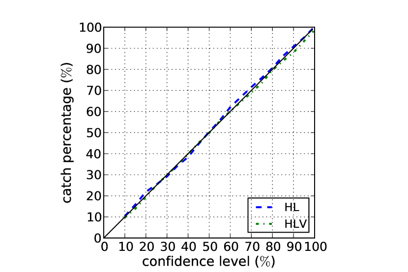
we find that the error in $R$ approximates a Gaussian with variance 

$$\sigma_{R_{ij}}^{2}=\frac{1}{\rho_{i}^{2}}+\frac{1}{\rho_{j}^{2}}.$$

Figure 1.— Cumulative $50\%$ confidence localization areas of the 630 simulated sources taken from  Singer et al. (2014) detected by LIGO Hanford+Livingston with the noise curve in LIGO-T1200307.

Figure 2.— Cumulative $50\%$ confidence localization areas of the 81 simulated sources taken from  Singer et al. (2014) detected by LIGO Hanford+Livingston and Virgo with the noise curves in LIGO-T1200307 and LIGO Scientific Collaboration et al. (2013). We only consider events with SNR greater than 4 in all three detectors.

Similar to the case with arrival times, there are $N-1$ independent SNR ratios from a network consisting of $N$ independent detectors. Therefore we define $R_{i}\equiv{\rm log}(\rho_{I}/\rho_{i}),\,i\neq I$ with an arbitrary reference detector I. The chi-square for SNR is then:

$$\chi^{2}_{\rho}(\theta,\phi,\iota,\psi)=\displaystyle\sum_{i,j}[\tilde{R_{i}}-R_{i}(\theta,\phi,\iota,\psi)]V^{-1}_{ij}[\tilde{R_{j}}-R_{j}(\theta,\phi,\iota,\psi)]$$ (14)

where $V_{ij}\equiv{\rm cov}(R_{i},R_{j})$ is the covariance matrix. If $i=j$ then

$$\sigma_{R_{i}R_{i}}^{2}=\frac{1}{\rho_{I}^{2}}+\frac{1}{\rho_{i}^{2}},$$

while if $i\neq j$ then we find:

$$\begin{split}\sigma^{2}_{R_{i}R_{j}}&=\frac{1}{2}[\sigma_{R_{i}}^{2}+\sigma_{R_{j}}^{2}-{\rm var}(R_{i}-R_{j})]\\ &=\frac{1}{2}(\sigma_{R_{i}}^{2}+\sigma_{R_{j}}^{2}-\sigma_{R_{ji}}^{2})\\ &=\frac{1}{2}\left(\frac{1}{\rho_{I}^{2}}+\frac{1}{\rho_{i}^{2}}+\frac{1}{\rho_{I}^{2}}+\frac{1}{\rho_{j}^{2}}-\frac{1}{\rho_{i}^{2}}-\frac{1}{\rho_{j}^{2}}\right)\\ &=\frac{1}{\rho_{I}^{2}}.\end{split}$$ (15)

By taking the logarithm of the power ratio (Eq. 13) we are able to estimate the covariance matrix analytically.

As shown in Eq. 14, the directional information is degenerate with binary inclination and orientation. We marginalize over $(\iota,\psi)$ using Eqs. 4 and 5:

$$\chi^{2}_{\rho}(\theta,\phi)=-2\,{\rm log}\left(\frac{1}{f(\theta,\phi)}\displaystyle\int e^{-\chi^{2}_{\rho}(\theta,\phi,\iota,\psi)/2}\,f(\theta,\phi,\iota,\psi)\,d\iota d\psi\right).$$ (16)

Figure 3.— We compare the improvement of using time of arrival+SNR and time of arrival+SNR+phase. The simulated sources were taken from  Singer et al. (2014) and localized with LIGO Hanford and Livingston.

The sky prior (Eq. 4) also contributes to the posterior, so we define the total chi-square as: $\chi^{2}(\theta,\phi)\equiv\chi^{2}_{\vec{\epsilon}}(\theta,\phi)-2\,{\rm log}\,f(\theta,\phi)$. We grid the sky uniformly in $({\rm cos}\,\theta,\phi)$ (or in $(\theta,\phi)$ when close to the poles) , calculate $\chi^{2}$ at each grid point, and then find the minimum $\chi^{2}_{\rm min}$ from which to determine $\Delta\chi^{2}$ at each point and establish the posterior (Eq. 1). We use a contour defined by $\Delta\chi^{2}=b_{p}$ to determine the boundary of the localization area, such that

$$\frac{1}{n}\displaystyle\int_{\Delta\chi^{2}(\theta,\phi)<b_{p}}e^{-\Delta\chi^{2}(\theta,\phi)/2}\,d\theta d\phi=p\,\%,$$ (17)

where $n$ normalizes the probability to 1. We vary the $\Delta\chi^{2}$ value of the boundary, $b_{p}$, until the integral in Eq. 17 reaches the desired confidence level $p\,\%$. If the posterior is Gaussian, we can calculate $b_{p}$ analytically. The sky prior (Eq. 4) and the marginalization (Eq. 16) break the Gaussianity. However, we still use contours of constant $\Delta\chi^{2}$ as the boundaries of our confidence level, where we explicitly compute the probability incorporated within each contour rather than assuming the analytic value appropriate for true Gaussian distributions (Press et al., 2007).

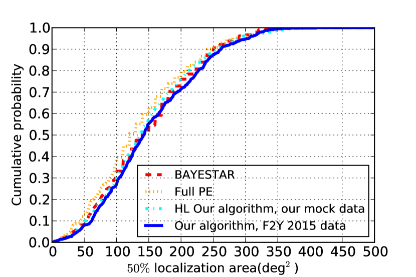
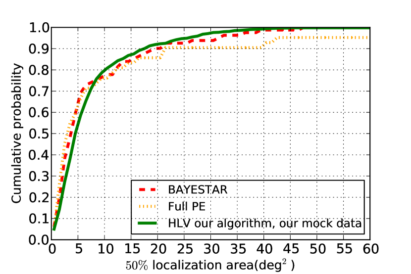
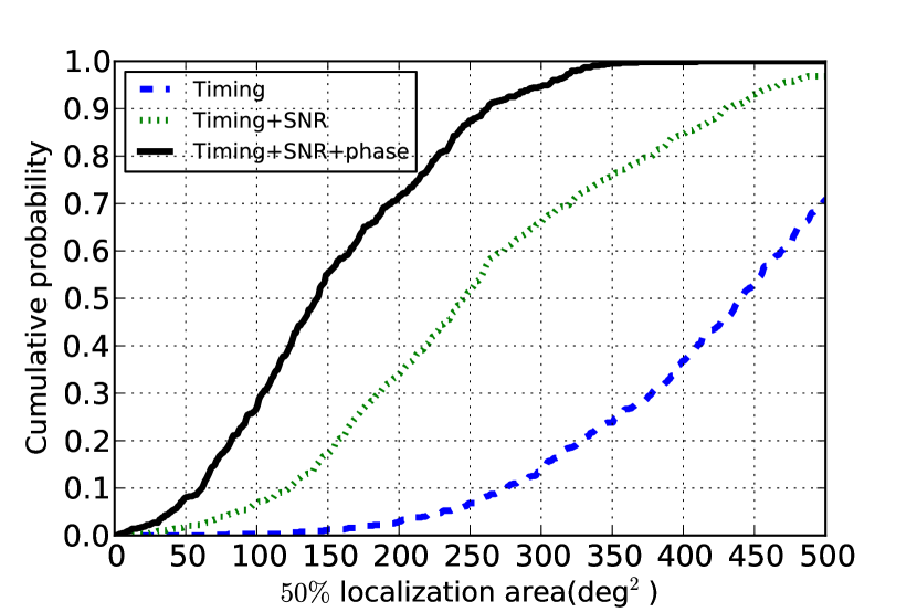
In summary, for a given event we use Eqs. 1, 6, and 17 to estimate the localization area on the sky. As a test, we apply our localization algorithm to the simulated source catalog from Singer et al. (2014), and compare our localization areas to those found from the BAYESTAR algorithm. As shown in Fig. 1, we find excellent consistency. We also explore the contribution to the localization determination arising from incorporating SNR and phase information in addition to timing, finding that the resulting localization areas decrease significantly (Fig. 3). In order to test our Bayesian posterior, we determine the fraction of binaries which fall within our localization areas, and compare this to the predicted percentages. Fig. 4 shows that our formalism is self consistent. In order to further study the properties of our low-latency localization algorithm, we simulate a population of binary neutron star. We follow the Monte Carlo approach we presented in Chen and Holz (2014), utilizing the same noise curve as Singer et al. (2014). For each binary we calculate the true SNR and time-of-arrival in each detector. We then add in Gaussian noise for each of these quantities, mimicking the actual measurements (ignoring glitches; we have assumed a threshold SNR of $\rho_{\rm th}=12$ to mimimize the importance of these). Our resulting distribution of localization areas is comparable to that in Figs. 1 and 2, indicating that our Monte Carlo sources and pipelines are consistent with that of Singer et al. (2014).

Figure 4.— Integrated confidence level versus the actual captured percentage. The samples were taken from  Singer et al. (2014) and localized with LIGO Hanford+Livingston (HL) and HL+Virgo (HLV). The black line is the $x=y$ line (perfect consistency). We find that the fraction of binaries found within our sky localization contours is in very good agreement with the predicted percentage.

3. Loudest Event

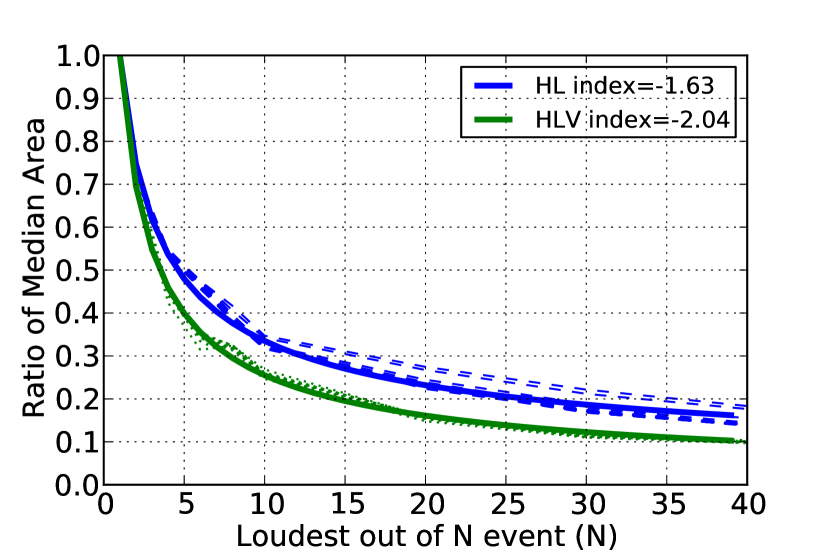
As shown in Fig. 1 and  2, there is a broad distribution of localization areas for any given set of sources. This is related to the broad distribution of measured SNRs of the sources, which is in turn related to the distribution of distances to the sources. If not all GW triggers can be followed, the louder (higher SNR) events offer the opportunity for better localization and more efficient follow-up. In Fig. 5 we show the median localization area of the loudest source out of $N$ events. The $N=1$ case corresponds to the full distribution of localization areas for all events (also seen in Fig. 1). From Fisher matrix calculations the localization area is expected to scale as Area$\sim{\rm SNR}^{-2}$. This is true for 3 or more detectors, while for 2 detectors the sky locations are generally poorly constrained within a broad timing ring and the localization area will scale more slowly with improving SNR. In our loudest event paper (Chen and Holz, 2014) we show that the distribution of detected SNRs follows a universal distribution. We also derive the universal loudest event distribution, which depends upon the detection threshold, $\rho_{\rm th}$, and the number of events, $N$. The cumulative probability is:

$$F_{\rho_{\rm max}}=\left(1-\left(\frac{\rho_{\rm th}}{\rho_{\rm max}}\right)^{3}\right)^{N}.$$ (18)

In (Chen and Holz, 2014) we pointed out that Eq. 18 is independent of the detector network, detector sensitivity, and all properties of the sources. Eq. 18 can applied to all situations (e.g. 2 or 3 detectors operating at different sensitivities looking for BNS, NS-BH, or supernovae), and we can predict the highest SNR out of $N$ detections analytically. For example, the median of this distribution is given by:

$$\rho_{\rm max}=\frac{\rho_{\rm th}}{(1-0.5^{1/N})^{1/3}}.$$

If the localization area scales as Area$\sim{\rm SNR}^{-2}$, we would expect the ratio between the median area of the loudest out of $N$ events, $A_{\rm max\,N}$, and the median area of all events ($N=1$), $A_{1}$, to scale as:

$$\frac{A_{\rm max\,N}}{A_{1}}=\left(\frac{\rho_{\rm max\,N}}{\rho_{1}}\right)^{-2}=\left(\frac{1-0.5^{1/N}}{0.5}\right)^{2/3}.$$ (19)

We fit for the area-SNR scaling index in Fig. 5. For 3 detectors we see that the area scales as SNR to the power of -2.04, while for the 2 detector case the scaling is shallower (-1.63) as expected.

Eq. 19 shows that the localization area shrinks rapidly as additional binaries are initially added: waiting for the loudest out of the first 4 events will reduce the expected sky area required for follow-up by a factor of 1.9 (2 detectors) and 2.2 (3 detectors). This improvement declines for larger sets of binaries; going from 4 to 10 binaries reduces the sky area by an additional factor of 1.6 (2 detectors) and 1.8 (3 detectors). This suggests that there may be an optimal strategy for selecting events for EM follow-up, based on the expected event rate and the observational constraints of the follow-up facility.

Figure 5.— Ratio between the median localization area for the loudest event out of $N$ detections and that for all events ($N=1$). The SNR of the loudest events can be estimated from Eq. 18. For 3 detectors (HLV) the areas roughly scale as SNR^-2 (index=-2.04), while for 2 detectors (HL) the scaling is shallower (index=-1.63).

4. GRB Joint Localizations

Short GRBs are thought to be the very bright EM counterpart of binary neutron star or neutron star-black hole coalescence (Kocevski et al., 2010; Fong et al., 2013; Fong and Berger, 2013). If a short GRB is accompanied by GW emission, joint GW+EM detection would confirm the binary nature of the short GRB engine as well as help constrain the binary parameters. For example, the existence of gamma-ray emission would suggest that at least one of the members of the binary is a neutron star, and measurements of the inclination would help constrain properties of the beamed jet. In addition, the shape and area of the localization of the GRB in gamma-rays is independent of the Advanced LIGO & Virgo localization, and thus combining the two localization areas can significantly constrain the sky position of the source.

We would like to explore the benefit to sky localization of a prior constraint on the inclination. Let us consider the case where a GRB has been observed, and we thereby have a prior on the GRB beaming angle which comes into Eqs. 4, 11, and 16. We randomly generate 3,000 binary neutron star mergers following the approach in Chen and Holz (2014). As suggested by observations, we assume that GRBs are beamed within the range $1$–$10^{\circ}$ (Soderberg et al., 2006; Burrows et al., 2006; Coward et al., 2012; Fong et al., 2012), and we confine the orientation of our binaries to be uniformly distributed in ${\rm cos}\,\iota$ within $\pm{\rm cos}\,1^{\circ},\;\pm{\rm cos}\,5^{\circ},\;\pm{\rm cos}\,10^{\circ}$ (3 samples of 1,000 binaries each). For each beaming angle distribution, we localize the source by marginalizing over the corresponding range of inclination angles (“$\sin\iota\leq\sin\theta_{j}$” which allows for both face-on and tail-on beaming; see Table 1) or over the full range of inclinations (“random $\iota$”). We then compare the localization area and summarize the results in Table 1. Using the beaming prior only improves the localization by $<10\%$, even in the case of $1^{\circ}$ beaming. This is due to the unknown direction of rotation; a clockwise binary produces a different phase pattern than a counter-clockwise binary, and knowing that a binary is almost face-on or almost tail-on is not as useful as knowing that a binary is definitely one or the other. If we assume that we break the clockwise/counter clockwise degeneracy, the localization improves significantly, approaching the “known $\iota$” case. It is to be noted that additional measurements of phase, e.g., from Virgo, LIGO-India, or KAGRA, do not help to break this degeneracy. This is because a clockwise binary “above” a detector produces an identical waveform to a counter-clockwise binary “below”. Alternatively, if the sky position is known, the GW network can determine whether the binary is orbiting clockwise or counter-clockwise.

$\theta_{j}$	known $\iota$	$\sin\iota\leq\sin\theta_{j}$	random $\iota$
1∘	340 deg2	490 deg2	540 deg2
5∘	340 deg2	500 deg2	530 deg2
10∘	350 deg2	510 deg2	530 deg2
10∘, clockwise	$\cdots$	350 deg2	$\cdots$

Table 1Hanford+Livingston median 90$\%$ localization area for binary neutron stars beamed within $\theta_{j}$. The localizations are for three different sets of priors: knowing the exact inclination (“known $\iota$”), knowing the beaming angle (“$\sin\iota\leq\sin\theta_{j}$”) but not whether it is clockwise or counter-clockwise, and assuming no information about beaming (“random $\iota$”). The last row corresponds to binaries that are beamed within $10^{\circ}$ and revolve in the clockwise direction on the sky, and where the prior assumes not only the beaming but also the clockwise direction.

Although a beaming prior is of limited utility in determining position, the contribution of an independent localization from EM measurements of a GRB can be significant. The Fermi Gamma-ray Burst Monitor (GBM) telescope has a field-of-view of 8 steradians. It observes $\sim 45$ short GRBs a year, potentially serving as a triggering system for binary mergers. A limitation of the Fermi GBM is that it can only localize sources within tens to hundreds of square degrees (Briggs et al., 2009). We conservatively assume that Fermi GBM localizes sources to a 100 deg² ($1\sigma$) 2D circular Gaussian. This independent likelihood function contributes to the posterior as an additional $\chi^{2}_{\rm Fermi}$. Fig. 6 shows the significant improvement in source localization which results from joint detections from Fermi and advanced GW detectors. The median of the 90% confidence ($\sim 2\sigma$) area for joint detection lies around 120 deg² even with only two GW detectors, as compared with 460 deg² and 560 deg² for the GRB and GW localizations, respectively. In this case the beaming priors make no difference whatsoever in the localization.

5. Discussion

We have developed a low latency localization algorithm for ground-based GW detector networks. Our approach requires the timing, phase, and SNR of the sources (provided by the detection pipeline), and within a fraction of a second produces a 2D localization. We have implemented our algorithm for the case of non-spinning compact binary coalescences, assuming representative output from the detection pipeline (GSTLAL); this can in principle be generalized to other (preferably modeled) burst sources. Although the sky location is degenerate with other physical properties (e.g. masses, distances, and spins of the binaries), our algorithm avoids the need to estimate these paramters by instead utilizing the difference in arrival times, difference in phases, and the ratio of measured SNRs. This increases the simplicity and speed of localization, while reducing potential errors. Imprecise waveforms can result in errors in the SNR measurements, but the ratio of SNRs between detectors is less sensitive to these errors. By taking the SNR ratio, the parameter space is highly reduced. For binary mergers, the two relevant unknowns are the binary orientation and inclination; it is computationally inexpensive to pre-calculate the marginalization of these over the entire sky . The timing and sky priors can also be pre-gridded and pre-calculated, simplifying the localization algorithm to a $\chi^{2}$ determination using a look-up table combined with direct summation. Once the tables are loaded into memory, the entire algorithm takes $<1$ second on a laptop (using a Python 2 script running on one thread on a 2.3 Ghz Intel Core i7). It would be straightforward to parallelize the algorithm (e.g., by having each core analyze a fraction of the sky), leading to sky localization within 0.1 seconds or better. There is ongoing work to speed up the detection pipeline  (Q. Chu, 2015), including the possibility of event detection before merger. This capability is only of use when coupled with rapid localization; our prompt and accurate algorithm offers the possibility of real-time localization contemporaneous with the inspiral and merger of the binary. It is to be noted that our algorithm can be generalized to calculate distance as well as sky position, allowing for the possibility of low-latency 3D localization.

Figure 6.— Cumulative distribution of sky localization for joint GW and Fermi GBM detections of short GRBs. This shows significant improvement, as compared with GW detection alone (Table 1).

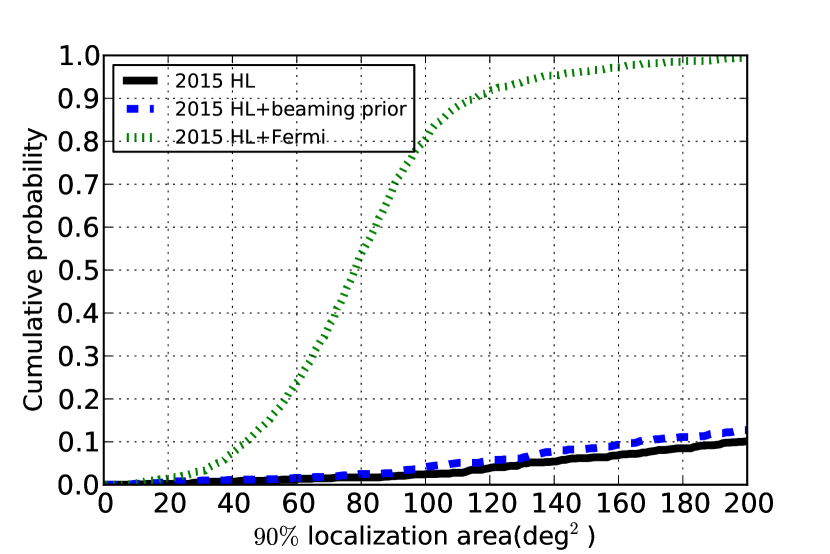
In Fig. 2 we show the cumulative distribution of $50\%$ localization areas for the first two years of advanced LIGO and Virgo network operation. Although the localization is significantly improved with the addition of Virgo (c.f. Fig. 1), these represent a minority ($\sim 25$%), since most events detected by this network have a Virgo SNR below the detection threshold ($\rho_{\rm V}<4$) due to Virgo’s lower sensitivity and mis-aligned antenna power pattern (Chen and Holz, 2014). Unless the detection pipeline produces information for these sub-threshold events, the low-latency localization will be based on information from only two detectors (i.e., H and L), followed by better localization resulting from the full parameter estimation pipeline analyzing the sub-threshold waveforms (Singer et al., 2014); we note that there is a potential remedy to this discussed in Section IX of Singer and Price (2015). For sources detected with only 2 detectors, the localization of events with the 2016 network is potentially worse than those detected in 2015 (Singer et al., 2014). This is because the effective bandwidth of the 2016 noise curve may be narrower than the 2015 case, leading to inferior localization for sources with the same measured SNRs (e.g., SNR=12). Of course, the 2016 network would detect sources from the 2015 network at higher SNR, and therefore would do a superior job of localizing identical sources. Occasionally the event will trigger only H+V or L+V. In these rare situations the localization will generally be worse than H+L, not only because Virgo operates at lower sensitivity, but also because the Virgo SNR distribution skews to lower values when coupled with an H or L detection (Chen and Holz, 2014).

We explore the dependence of localization on SNR, confirming that high SNR events lead to better localization. Since there is a universal distribution of SNR, we can use this to estimate the benefit of waiting for loud events. Fig. 5 shows that waiting for the loudest out of the first 4 events shrinks the median localization area by a factor of almost 2.

Fig. 6 shows that combining an EM prior on the sky location of a source with GW localization greatly improves the resulting localization. This is because the shapes of the two localization regions are ver different and completely uncorrelated. Fermi GBM detection of a short GRB would then greatly enhance the localization resulting from a GW network. One might have thought that such a detection would also place useful prior constraints on the beaming angle (i.e., gamma-ray detection implies that the binary is face-on). However, Table 1 and Fig. 6 demonstrate that the beaming prior makes only a marginal improvement in localization because of the degeneracy between face-on and tail-on binaries.

We have developed a simple, fast, and accurate algorithm for the localization of GW sources. This algorithm, when coupled with a fast detection pipeline, can play an important role in the development of multi-messenger astronomy.

References

- Metzger and Berger (2012) B. D. Metzger and E. Berger, ApJ 746, 48 (2012), 1108.6056.
- Chen and Holz (2013) H.-Y. Chen and D. E. Holz, Physical Review Letters 111, 181101 (2013), 1206.0703.
- Kocevski et al. (2010) D. Kocevski, C. C. Thöne, E. Ramirez-Ruiz, J. S. Bloom, J. Granot, N. R. Butler, D. A. Perley, M. Modjaz, W. H. Lee, B. E. Cobb, et al., Mon. Not. R. Astron. Soc. 404, 963 (2010), 0908.0030.
- Fong et al. (2013) W. Fong, E. Berger, R. Chornock, R. Margutti, A. J. Levan, N. R. Tanvir, R. L. Tunnicliffe, I. Czekala, D. B. Fox, D. A. Perley, et al., ApJ 769, 56 (2013), 1302.3221.
- Fong and Berger (2013) W. Fong and E. Berger, ApJ 776, 18 (2013), 1307.0819.
- Berger et al. (2013) E. Berger, W. Fong, and R. Chornock, Astrophys. J. Lett. 774, L23 (2013), 1306.3960.
- Tanvir et al. (2013) N. R. Tanvir, A. J. Levan, A. S. Fruchter, J. Hjorth, R. A. Hounsell, K. Wiersema, and R. L. Tunnicliffe, Nature 500, 547 (2013), 1306.4971.
- Freiburghaus et al. (1999) C. Freiburghaus, S. Rosswog, and F.-K. Thielemann, Astrophys. J. Lett. 525, L121 (1999).
- Metzger et al. (2010) B. D. Metzger, G. Martínez-Pinedo, S. Darbha, E. Quataert, A. Arcones, D. Kasen, R. Thomas, P. Nugent, I. V. Panov, and N. T. Zinner, Mon. Not. R. Astron. Soc. 406, 2650 (2010), 1001.5029.
- Harry and LIGO Scientific Collaboration (2010) G. M. Harry and LIGO Scientific Collaboration, Classical and Quantum Gravity 27, 084006 (2010).
- LIGO Scientific Collaboration et al. (2013) LIGO Scientific Collaboration, Virgo Collaboration, J. Aasi, J. Abadie, B. P. Abbott, R. Abbott, T. D. Abbott, M. Abernathy, T. Accadia, F. Acernese, et al., ArXiv e-prints (2013), 1304.0670.
- Accadia (2012) T. e. a. Accadia, Virgo Document VIR-0128A-12 (2012).
- Fairhurst (2009) S. Fairhurst, New Journal of Physics 11, 123006 (2009), 0908.2356.
- Fairhurst (2011) S. Fairhurst, Classical and Quantum Gravity 28, 105021 (2011), 1010.6192.
- Singer and Price (2015) L. P. Singer and L. R. Price, ArXiv e-prints (2015), 1508.03634.
- Kasliwal and Nissanke (2014) M. M. Kasliwal and S. Nissanke, Astrophys. J. Lett. 789, L5 (2014), 1309.1554.
- Sidery et al. (2014) T. Sidery, B. Aylott, N. Christensen, B. Farr, W. Farr, F. Feroz, J. Gair, K. Grover, P. Graff, C. Hanna, et al., Phys. Rev. D 89, 084060 (2014), 1312.6013.
- Singer et al. (2014) L. P. Singer, L. R. Price, B. Farr, A. L. Urban, C. Pankow, S. Vitale, J. Veitch, W. M. Farr, C. Hanna, K. Cannon, et al., ApJ 795, 105 (2014), 1404.5623.
- Veitch et al. (2015) J. Veitch, V. Raymond, B. Farr, W. Farr, P. Graff, S. Vitale, B. Aylott, K. Blackburn, N. Christensen, M. Coughlin, et al., Phys. Rev. D 91, 042003 (2015), 1409.7215.
- Aasi et al. (2013) J. Aasi, J. Abadie, B. P. Abbott, R. Abbott, T. D. Abbott, M. Abernathy, T. Accadia, F. Acernese, C. Adams, T. Adams, et al., Phys. Rev. D 88, 062001 (2013), 1304.1775.
- Chen and Holz (2014) H.-Y. Chen and D. E. Holz, ArXiv e-prints (2014), 1409.0522.
- Sathyaprakash and Schutz (2009) B. S. Sathyaprakash and B. F. Schutz, Living Reviews in Relativity 12, 2 (2009), 0903.0338.
- Schutz (2011) B. F. Schutz, Classical and Quantum Gravity 28, 125023 (2011), 1102.5421.
- Berry et al. (2015) C. P. L. Berry, I. Mandel, H. Middleton, L. P. Singer, A. L. Urban, A. Vecchio, S. Vitale, K. Cannon, B. Farr, W. M. Farr, et al., ApJ 804, 114 (2015), 1411.6934.
- Grover et al. (2014) K. Grover, S. Fairhurst, B. F. Farr, I. Mandel, C. Rodriguez, T. Sidery, and A. Vecchio, Phys. Rev. D 89, 042004 (2014), 1310.7454.
- Cutler and Flanagan (1994) C. Cutler and É. E. Flanagan, Phys. Rev. D 49, 2658 (1994), gr-qc/9402014.
- Press et al. (2007) W. H. Press, S. A. Teukolsky, W. T. Vetterling, and B. P. Flannery, Numerical Recipes 3rd Edition: The Art of Scientific Computing (Cambridge University Press, New York, NY, USA, 2007), 3rd ed., ISBN 0521880688, 9780521880688.
- Soderberg et al. (2006) A. M. Soderberg, E. Berger, M. Kasliwal, D. A. Frail, P. A. Price, B. P. Schmidt, S. R. Kulkarni, D. B. Fox, S. B. Cenko, A. Gal-Yam, et al., ApJ 650, 261 (2006), arXiv:astro-ph/0601455.
- Burrows et al. (2006) D. N. Burrows, D. Grupe, M. Capalbi, A. Panaitescu, S. K. Patel, C. Kouveliotou, B. Zhang, P. Mészáros, G. Chincarini, N. Gehrels, et al., ApJ 653, 468 (2006), arXiv:astro-ph/0604320.
- Coward et al. (2012) D. Coward, E. Howell, T. Piran, G. Stratta, M. Branchesi, O. Bromberg, B. Gendre, R. Burman, and D. Guetta, arXiv:1202.2179 (2012).
- Fong et al. (2012) W. Fong, E. Berger, R. Margutti, B. A. Zauderer, E. Troja, I. Czekala, R. Chornock, N. Gehrels, T. Sakamoto, D. B. Fox, et al., arXiv:1204.5475 (2012).
- Briggs et al. (2009) M. S. Briggs, V. Connaughton, C. A. Meegan, C. Wilson-Hodge, M. Kippen, and K. Hurley, in American Institute of Physics Conference Series, edited by C. Meegan, C. Kouveliotou, and N. Gehrels (2009), vol. 1133 of American Institute of Physics Conference Series, pp. 40–42.
- Q. Chu (2015) L. W. Q. Chu, E. Howell, LIGO Document P1500132-v1 (2015).