Parameter estimation for compact binaries with ground-based gravitational-wave observations using LALInference

Abstract

The Advanced LIGO and Advanced Virgo gravitational wave (GW) detectors will begin operation in the coming years, with compact binary coalescence events a likely source for the first detections. The gravitational waveforms emitted directly encode information about the sources, including the masses and spins of the compact objects. Recovering the physical parameters of the sources from the GW observations is a key analysis task. This work describes the LALInference software library for Bayesian parameter estimation of compact binary signals, which builds on several previous methods to provide a well-tested toolkit which has already been used for several studies.

We show that our implementation is able to correctly recover the parameters of compact binary signals from simulated data from the advanced GW detectors. We demonstrate this with a detailed comparison on three compact binary systems: a binary neutron star (BNS), a neutron star – black hole binary (NSBH) and a binary black hole (BBH), where we show a cross-comparison of results obtained using three independent sampling algorithms. These systems were analysed with non-spinning, aligned spin and generic spin configurations respectively, showing that consistent results can be obtained even with the full 15-dimensional parameter space of the generic spin configurations.

We also demonstrate statistically that the Bayesian credible intervals we recover correspond to frequentist confidence intervals under correct prior assumptions by analysing a set of 100 signals drawn from the prior.

We discuss the computational cost of these algorithms, and describe the general and problem-specific sampling techniques we have used to improve the efficiency of sampling the compact binary coalescence (CBC) parameter space.

I Introduction

The direct observation of GWs and the study of relativistic sources in this new observational window is the focus of a growing effort with broad impact on astronomy and fundamental physics. The network of GW laser interferometers – LIGO Abbott et al. (2009), Virgo Acernese et al. (2008) and GEO 600 Grote (2010) – completed science observations in initial configuration in 2010, setting new upper-limits on a broad spectrum of GW sources. At present, LIGO and Virgo are being upgraded to their advanced configurations Harry and the LIGO Scientific Collaboration (2010); Virgo Collaboration (2009), a new Japanese interferometer, KAGRA (formerly known as the Large-Scale Gravitational-wave Telescope, LCGT) Kuroda (2011) is being built, and plans are underway to relocate one of the LIGO instruments upgraded to Advanced LIGO sensitivity to a site in India (LIGO-India) Unnikrishnan (2013). Advanced LIGO is currently on track to resume science observations in 2015 with Advanced Virgo following soon after gw_ (2013); around the turn of the decade LIGO-India and KAGRA should also join the network of ground-based instruments.

Along with other possible sources, advanced ground-based interferometers are expected to detect GWs generated during the last seconds to minutes of life of extra-galactic compact binary systems, with neutron star and/or black hole component masses in the range $\sim 1\,\mathrm{M}_{\odot}-100\,\mathrm{M}_{\odot}$. The current uncertainties on some of the key physical processes that affect binary formation and evolution are reflected in the expected detection rate, which spans three orders of magnitude. However, by the time interferometers operate at design sensitivity, between one observation per few years and hundreds of observations per year are anticipated gw_ (2013); Abadie et al. (2010), opening new avenues for studies of compact objects in highly relativistic conditions.

During the approximately ten years of operation of the ground-based GW interferometer network, analysis development efforts for binary coalescences have been focused on the detection problem, and rightly so: how to unambiguously identify a binary coalescence in the otherwise overwhelming instrumental noise. The most sensitive compact binary searches are based on matched-filtering techniques, and are designed to keep up with the data rate and promptly identify detection candidates Babak et al. (2013); Cannon et al. (2012). A confirmation of the performance of detection pipelines has been provided by the “blind injection challenge” in which a synthetic compact binary coalescence signal was added (unknown to the analysis teams) to the data stream and successfully detected Abadie et al. (2012).

Once a detection candidate has been isolated, the next step of the analysis sequence is to extract full information regarding the source parameters and the underlying physics. With the expected detection of GWs in the coming years, this part of the analysis has become the focus of a growing number of studies.

The conceptual approach to inference on the GW signal is deeply rooted in the Bayesian framework. This framework makes it possible to evaluate the marginalized posterior probability density functions (PDFs) of the unknown parameters that describe a given model of the data and to compute the so-called evidence of the model itself. It is well known that Bayesian inference is computationally costly, making the efficiency of the PDF and evidence calculations an important issue. For the case of coalescing binary systems the challenge comes from many fronts: the large number of unknown parameters that describe a model (15 parameters to describe a gravitational waveform emitted by a binary consisting of two point masses in a circular orbit assuming that general relativity is accurate, plus other model parameters to account for matter effects in the case of neutron stars, the noise, instrument calibration, etc.), complex multi-modal likelihood functions, and the computationally intensive process of generating waveforms.

Well known stochastic sampling techniques – Markov chain Monte Carlo Christensen and Meyer (2001); Christensen et al. (2004); Röver et al. (2006, 2007); van der Sluys et al. (2008a, b); Raymond et al. (2009); van der Sluys et al. (2009); Raymond et al. (2010), Nested Sampling Skilling (2006); Veitch and Vecchio (2010) and MultiNest/BAMBI Feroz and Hobson (2008); Feroz et al. (2009, 2013); Graff et al. (2012) – have been used in recent years to develop algorithms for Bayesian inference on GW data aimed at studies of coalescing binaries. An underlying theme of this work has been the comparison of these sampling techniques and the cross-validation of results with independent algorithms. In parallel, the inference effort has benefited from a number of advances in other areas that are essential to maximise the science exploitation of detected GW signals, such as waveform generation and standardised algorithms and libraries for the access and manipulation of GW data. The initially independent developments have therefore progressively converged towards dedicated algorithms and a common infrastructure for Bayesian inference applied to GW observations, specifically for coalescing binaries but applicable to other sources. These algorithms and infrastructure are now contained in a dedicated software package: LALInference.

The goal of this paper is to describe LALInference. We will cover the details of our implementation, designed to overcome the problems faced in performing Bayesian inference for GW observations of CBC signals. This includes three independent sampling techniques which were cross-compared to provide confidence in the results that we obtain for CBC signals, and compared with known analytical probability distributions. We describe the post-processing steps involved in converting the output of these algorithms to meaningful physical statements about the source parameters in terms of credible intervals. We demonstrate that these intervals are well-calibrated measures of probability through a Monte Carlo simulation, wherein we confirm the quoted probability corresponds to frequency under correct prior assumptions. We compare the computational efficiency of the different methods and mention further enhancements that will be required to take full advantage of the advanced GW detectors.

The LALInference software consists of a C library and several post-processing tools written in python. It leverages the existing LSC Algorithm Library (LAL) to provide

• Standard methods of accessing GW detector data, using LAL methods for estimating the power spectral density (PSD), and able to simulate stationary Gaussian noise with a given noise curve.

• the ability to use all the waveform approximants included in LAL that describe the evolution of point-mass binary systems, and waveforms under development to account for matter effects in the evolution of binary neutron stars and generalisations of waveforms beyond general relativity;

• Likelihood functions for the data observed by a network of ground-based laser interferometers given a waveform model and a set of model parameters;

• Three independent stochastic sampling techniques of the parameter space to compute PDFs and evidence;

• Dedicated “jump proposals” to efficiently select samples in parameter space that take into account the specific structure of the likelihood function;

• Standard post-processing tools to generate probability credible regions for any set of parameters.

During the several years of development, initial implementations of these Bayesian inference algorithms and LALInference have been successfully applied to a variety of problems, such as the impact of different network configurations on parameter estimation Veitch et al. (2012), the ability to measure masses and spins of compact objects Rodriguez et al. (2014); van der Sluys et al. (2008a); Vitale et al. (2014), to reconstruct the sky location of a detected GW binary Raymond et al. (2009); Blackburn et al. (2013); Grover et al. (2014) and the equation of state of neutron stars Del Pozzo et al. (2013a), the effects of calibration errors on information extraction Vitale et al. (2012) and tests of general relativity Del Pozzo et al. (2011); Li et al. (2012); Agathos et al. (2014). Most notably LALInference has been at the heart of the study of detection candidates, including the blind injection, during the last LIGO/Virgo science run Aasi et al. (2013), and has been used for the Numerical INJection Analysis project NINJA2 Aasi et al. (2014). It has been designed to be flexible in the choice of signal model, allowing it to be adapted for analysis of signals other than compact binaries, including searches for continuous waves Pitkin et al. (2012), and comparison of core-collapse supernova models based on Logue et al. (2012).

The paper is organised as follows: Section II provides a summary of the key concepts of Bayesian inference, and specific discussion about the many waveform models that can be used in the analysis and the relevant prior assumptions. In Section III we describe the conceptual elements concerning the general features of the sampling techniques that are part of LALInference: Markov chain Monte Carlo, Nested Sampling and MultiNest/BAMBI. Section IV deals with the problem of providing marginalized probability functions and (minimum) credible regions at a given confidence level from a finite number of samples, as is the case of the outputs of these algorithms. In Section V we summarise the results from extensive tests and validations that we have carried out by presenting representative results on a set of injections in typical regions of the parameter space, as well as results obtained by running the algorithms on known distributions. This section is complemented by Section VI in which we consider efficiency issues, and we report the run-time necessary for the analysis of coalescing binaries in different cases; this provides a direct measure of the latency timescale over which fully coherent Bayesian inference results for all the source parameters will be available after a detection candidate is identified. Section VII contains our conclusions and pointers to future work.

II Bayesian Analysis

We can divide the task of performing inference about the GW source into two problems: using the observed data to constrain or estimate the unknown parameters of the source  under a fixed model of the waveform (parameter estimation), and deciding which of several models is more probable in light of the observed data, and by how much (model selection). We tackle both these problems within the formalism of Bayesian inference, which describes the state of knowledge about an uncertain hypothesis $H$ as a probability, denoted $P(H)\in[0,1]$, or about an unknown parameter as a probability density, denoted $p(\theta|H)$, where $\int p(\theta|H)\mathrm{d}\theta=1$. Parameter estimation can then be performed using Bayes’ theorem, where a prior probability distribution $p(\theta|H)$ is updated upon receiving the new data $d$ from the experiment to give a posterior distribution $p(\theta|d,H)$,

$$p(\theta|d,H)=\frac{p(\theta|H)p(d|\theta,H)}{p(d|H)}.$$ (1)

Models typically have many parameters, which we collectively indicate with $\bm{\theta}=\{\theta_{1},\theta_{2},\ldots,\theta_{N}\}$. The joint probability distribution on the multi-dimensional space $p(\bm{\theta}|d,H)$ describes the collective knowledge about all parameters as well as their relationships. Results for a specific parameter are found by marginalising over the unwanted parameters,

$$p(\theta_{1}|d,H)=\int\mathrm{d}\theta_{2}\ldots\mathrm{d}\theta_{N}p(\bm{\theta}|d,H)\,.$$ (2)

The probability distribution can be used to find the expectation of various functions given the distribution, e.g. the mean

$$\left<\theta_{i}\right>=\int\theta_{i}p(\theta_{i}|d,H)\mathrm{d}\theta_{i}\,,$$ (3)

and credible regions, an interval in parameter space that containing a given probability (see Section  IV).

Model selection is performed by comparing the fully marginalized likelihood, or ‘evidence’, for different models. The evidence, usually denoted $Z$, is simply the integral of the likelihood, $L(d|\bm{\theta})=p(d|\bm{\theta},H)$, multiplied by the prior over all parameters of the model $H$,

$$Z=p(d|H)=\int\mathrm{d}\theta_{1}\ldots\mathrm{d}\theta_{N}~{}p(d|\bm{\theta},H)p(\bm{\theta}|H).$$ (4)

This is the normalisation constant that appears in the denominator of Eq. (1) for a particular model. Because we cannot exhaustively enumerate the set of exclusive models describing the data, we typically compare two competing models. To do this, one computes the ratio of posterior probabilities

$$O_{ij}=\frac{P(H_{i}|d)}{P(H_{j}|d)}=\frac{P(H_{i})}{P(H_{j})}\times\frac{Z_{i}}{Z_{j}}$$ (5)

where $B_{ij}=Z_{i}/Z_{j}$ is the ‘Bayes Factor’ between the two competing models $i$ and $j$, which shows how much more likely the observed data $d$ is under model $i$ rather than model $j$.

While the Bayesian methods described above are conceptually simple, the practical details of performing an analysis depend greatly on the complexity and dimensionality of the model, and the amount of data that is analysed. The size of the parameter space and the amount of data to be considered mean that the resulting probability distribution cannot tractably be analysed through a fixed sampling of the parameter space. Instead, we have developed methods for stochastically sampling the parameter space to solve the problems of parameter estimation and model selection, based on the Markov chain Monte Carlo (MCMC) and Nested Sampling techniques, the details of which are described in section III. Next we will describe the models used for the noise and the signal.

II.1 Data model

The data obtained from the detector is modelled as the sum of the compact binary coalescence signal $\bm{h}$ (described in section II.2) and a noise component $\bm{n}$,

$$\bm{d}=\bm{h}+\bm{n}.$$ (6)

Data from multiple detectors in the network are analysed coherently, by calculating the strain that would be observed in each detector:

$$\bm{h}=F_{+}(\alpha,\delta,\psi)\bm{h}_{+}+F_{\times}(\alpha,\delta,\psi)\bm{h}_{\times}$$ (7)

where $\bm{h}_{+,\times}$ are the two independent GW polarisation amplitudes and $F_{+,\times}(\alpha,\delta,\psi)$ are the antenna response functions ((e.g. Anderson et al., 2001)) that depend on the source location and the polarisation of the waves. Presently we ignore the time dependence of the antenna response function due to the rotation of the Earth, instead assuming that it is constant throughout the observation period. This is justifiable for the short signals considered here. Work is ongoing to include this time dependence when analysing very long signals with a low frequency cutoff below $40$ Hz, to fully exploit the advanced detector design sensitivity curves. The waveforms $\bm{h}_{+,\times}$ are described in Section II.2.

As well as the signal model, which is discussed in the next section, we must include a description of the observed data, including the noise, which is used to create the likelihood function. This is where knowledge of the detectors’ sensitivity and the data processing procedures are folded into the analysis.

We perform all of our analyses using the calibrated strain output of the GW detectors, or a simulation thereof. This is a set of time-domain samples $d_{i}$ sampled uniformly at times $t_{i}$, which we sometimes write as a vector $\bm{d}$ for convenience below. To reduce the volume of data, we down-sample the data from its original sampling frequency ($16384$ Hz) to a lower rate $f_{s}\geq 2f_{\rm max}$, which is high enough to contain the maximum frequency $f_{\rm max}$ of the lowest mass signal allowed by the prior, typically $f_{s}=4096$ Hz when analysing the inspiral part of a BNS signal. To prevent aliasing the data is first low-pass filtered with a 20th order Butterworth filter with attenuation of 0.1 at the new Nyquist frequency, using the implementation in LAL LAL , which preserves the phase of the input. We wish to create a model of the data that can be used to perform the analysis. In the absence of a signal, the simplest model which we consider is that of Gaussian, stationary noise with a certain power spectral density $S_{n}(f)$ and zero mean. $S_{n}(f)$ can be estimated using the data adjacent to the segment of interest, which is normally selected based on the time of coalescence $t_{c}$ of a candidate signal identified by a search pipeline. The analysis segment $\bm{d}$ spans the period $[t_{c}-T+2,t_{c}+2]$, i.e. a time $T$ which ends two seconds after the trigger (the 2 s safety margin after $t_{c}$ allows for inaccuracies in the trigger time reported by the search, and should encompass any merger and ringdown component of the signal). To obtain this estimate, by default we select a period of time (1024 s normally, but shorter if less science data is available) from before the time of the trigger to be analysed, but ending not later than $t_{c}-T$, so it should not contain the signal of interest. This period is divided into non-overlapping segments of the same duration $T$ as the analysis segment, which are then used to estimate the PSD. Each segment is windowed using a Tukey window with a 0.4 s roll-off, and its one-sided noise power spectrum is computed. For each frequency bin the median power over all segments is used as an estimate of the PSD in that bin. We follow the technique of Allen et al. (2012) by using the median instead of the mean to provide some level of robustness against large outliers occurring during the estimation time.

The same procedure for the PSD estimation segments is applied to the analysed data segment before it is used for inference, to ensure consistency.

For each detector we assume the noise is stationary, and characterised only by having zero mean and a known variance (estimated from the power spectrum). Then the likelihood function for the noise model is simply the product of Gaussian distributions in each frequency bin

$$p(\bm{d}|H_{N},S_{n}(f))=\exp\sum_{i}\left[-\frac{2|\tilde{d}_{i}|^{2}}{TS_{n}(f_{i})}-\frac{1}{2}\log(\pi TS_{n}(f_{i})/2)\right],$$ (8)

where $\tilde{\bm{d}}$ is the discrete Fourier transform of $\bm{d}$

$$\tilde{d}_{j}=\frac{T}{N}\sum_{k}d_{k}\exp(-2\pi ijk/N).$$ (9)

The presence of an additive signal $\bm{h}$ in the data simply adjusts the mean value of the distribution, so that the likelihood including the signal is

$$p(\bm{d}|H_{S},S_{n}(f),\bm{\theta}) =\exp\sum_{i}\left[-\frac{2|\tilde{h}_{i}(\bm{\theta})-\tilde{d}_{i}|^{2}}{TS_{n}(f_{i})}\right.$$

$$-\left.\frac{1}{2}\log(\pi TS_{n}(f_{i})/2)\right].$$ (10)

To analyse a network of detectors coherently, we make the further assumption that the noise is uncorrelated in each. This allows us to write the coherent network likelihood for data obtained from each detector as the product of the likelihoods in each detector Finn (1996).

$$p(\bm{d}_{\{H,L,V\}}|H_{S},{S_{n}}_{\{H,L,V\}}(f))=\prod_{i\in\{H,L,V\}}p(\bm{d}_{i}|H_{S},{S_{n}}_{i}(f))$$ (11)

This gives us the default likelihood function which is used for our analyses, and has been used extensively in previous work.

II.1.1 Marginalising over uncertainty in the PSD estimation

Using a fixed estimate of the PSD, taken from times outside the segment being analysed, cannot account for slow variations in the shape of the spectrum over timescales of minutes. We can model our uncertainty in the PSD estimate by introducing extra parameters into the noise model which can be estimated along with the signal parameters; we follow the procedure described in Littenberg et al. (2013). We divide the Fourier domain data into $\sim 8$ logarithmically spaced segments, and in each segment $j$, spanning $N_{j}$ frequency bins, introduce a scale parameter $\eta_{j}(f_{i})$ which modifies the PSD such that $S_{n}(f_{i})\rightarrow S_{n}(f_{i})\eta_{j}$ for $i_{j}<i\leq i_{j+1}$, where the scale parameter is constant within a frequency segment. With these additional degrees of freedom included in our model, the likelihood becomes

$$p(\bm{d}|H_{S},S_{n}(f),\bm{\theta},\bm{\eta}) =\exp\sum_{i}\left[-\frac{2|\tilde{h}_{i}(\bm{\theta})-\tilde{d}_{i}|^{2}}{T\eta(f_{i})S_{n}(f_{i})}\right.$$

$$\left.-\frac{1}{2}\log(\pi\eta_{i}TS_{n}(f_{i})/2)\right].$$ (12)

The prior on $\eta_{j}$ is a normal distribution with mean 1 and variance $1/N_{j}$. In the limit $N_{j}\rightarrow 1$ (i.e., there is one scale parameter for each Fourier bin), replacing the Gaussian prior with an inverse chi-squared distribution and integrating $p(d|H_{S},S_{n}(f),\bm{\theta},\bm{\eta})\times p(\bm{\theta},\bm{\eta}|H_{S},S_{n}(f))$ over $\bm{\eta}$, we would recover the Student’s t-distribution likelihood considered for GW data analysis in Röver et al. (2011); Röver (2011). For a thorough discussion of the relative merits of Student’s t-distribution likelihood and the approach used here, as well as examples which show how including $\bm{\eta}$ in the model improves the robustness of parameter estimation and model selection results, see Littenberg et al. (2013). In summary, the likelihood adopted here offers more flexibility given how much the noise can drift between the data used for estimating the PSD and the data being analysed. Further improvements on this scheme using more sophisticated noise models are under active development.

II.2 Waveform models

There are a number of different models for the GW signal that is expected to be emitted during a compact-binary merger. These models, known as waveform families, differ in their computational complexity, the physics they simulate, and their regime of applicability. LALInference  has been designed to easily interface with arbitrary waveform families.

Each waveform family can be thought of as a function that takes as input a parameter vector $\bm{\theta}$ and produces as output $\bm{h}_{+,\times}(\bm{\theta})$, either a time domain $h(\bm{\theta};t)$ or frequency-domain $h(\bm{\theta};f)$ signal. The parameter vector $\bm{\theta}$ generally includes at least nine parameters:

• Component masses $m_{1}$ and $m_{2}$. We use a reparametrisation of the mass plane into the chirp mass,

  $$\mathcal{M}=(m_{1}m_{2})^{3/5}(m_{1}+m_{2})^{-1/5}$$ (13)

  and the asymmetric mass ratio

  $$q=m_{2}/m_{1},$$ (14)

  as these variables tend to be less correlated and easier to sample. We use the convention $m_{1}\geq m_{2}$ when labelling the components. The prior is transformed accordingly (see figure 1). Another possible parametrisation is the symmetric mass ratio

  $$\eta=\frac{(m_{1}m_{2})}{(m_{1}+m_{2})^{2}}$$ (15)

  although we do not use this when sampling the distribution since the Jacobian of the transformation to $m_{1},m_{2}$ coordinates becomes singular at $m_{1}=m_{2}$.

• The luminosity distance to the source $d_{L}$;

• The right ascension $\alpha$ and declination $\delta$ of the source;

• The inclination angle $\iota$, between the system’s orbital angular momentum and the line of sight. For aligned- and non-spinning systems this coincides with the angle $\theta_{JN}$ between the total angular momentum and the line of sight (see below). We will use the more general $\theta_{JN}$ throughout the text.

• The polarisation angle $\psi$ which describes the orientation of the projection of the binary’s orbital momentum vector onto the plane on the sky, as defined in Anderson et al. (2001);

• An arbitrary reference time $t_{c}$, e.g. the time of coalescence of the binary;

• The orbital phase $\phi_{c}$ of the binary at the reference time $t_{c}$.

Nine parameters are necessary to describe a circular binary consisting of point-mass objects with no spins. If spins of the binary’s components are included in the model, they are described by six additional parameters, for a total of 15:

• dimensionless spin magnitudes $a_{i}$, defined as $a_{i}\equiv{|\bm{s_{i}}|}/{m_{i}^{2}}$ and in the range $[0,1]$, where $\bm{s_{i}}$ is the spin vector of the object $i$, and

• two angles for each $\bm{s_{i}}$ specifying its orientation with respect to the plane defined by the line of sight and the initial orbital angular momentum.

In the special case when spin vectors are assumed to be aligned or anti-aligned with the orbital angular momentum, the four spin-orientation angles are fixed, and the spin magnitudes alone are used, with positive (negative) signs corresponding to aligned (anti-aligned) configurations, for a total of 11 parameters. In the case of precessing waveforms, the system-frame parametrisation has been found to be more efficient than the radiation frame typically employed for parameter estimation of precessing binaries. The orientation of the system and its spinning components are parameterised in a more physically intuitive way that concisely describes the relevant physics, and defines evolving quantities at a reference frequency of $100$ Hz, near the peak sensitivity of the detectors Farr et al. (2014):

• $\theta_{JN}$: The inclination of the system’s total angular momentum with respect to the line of sight;

• $t_{1},t_{2}$: Tilt angles between the compact objects’ spins and the orbital angular momentum;

• $\phi_{12}$: The complimentary azimuthal angle separating the spin vectors;

• $\phi_{\rm JL}$: The azimuthal position of the orbital angular momentum on its cone of precession about the total angular momentum.

Additional parameters are necessary to fully describe matter effects in systems involving a neutron star, namely the equation of state Del Pozzo et al. (2013b), or to model deviations from the post-Newtonian expansion of the waveforms (e.g. Yunes and Pretorius, 2009; Li et al., 2012), but we do not consider these here. Finally, additional parameters could be used to describe waveforms from eccentric binaries Konigsdorffer and Gopakumar (2006) but these have not yet been included in our models.

GWs emitted over the whole coalescence of two compact objects produce a characteristic “chirp” of increasing amplitude and frequency during the adiabatic inspiral phase, followed by a broad-band merger phase and then damped quasi-sinusoidal signals during the ringdown phase. The characteristic time and frequency scales of the whole inspiral-merger-ringdown are important in choosing the appropriate length of the data segment to analyse and the bandwidth necessary to capture the whole radiation. At the leading Newtonian quadrupole order, the time to coalescence of a binary emitting GWs at frequency $f$ is Allen et al. (2012):

$$\tau=93.9\left(\frac{f}{30\,\mathrm{Hz}}\right)^{-8/3}\,\left(\frac{\mathcal{M}}{0.87\,M_{\odot}}\right)^{-5/3}\,\mathrm{sec}\,.$$ (16)

Here we have normalised the quantities to an $m_{1}=m_{2}=1\,M_{\odot}$ equal mass binary. The frequency of dominant mode gravitational wave emission at the innermost stable circular orbit for a binary with non-spinning components is Allen et al. (2012):

$$f_{\mathrm{isco}} =\frac{1}{6^{3/2}\pi(m_{1}+m_{2})}=4.4\left(\frac{M_{\odot}}{m_{1}+m_{2}}\right)\,\mathrm{kHz}\,,$$ (17)

The low-frequency cut-off of the instrument, which sets the duration of the signal, was 40 Hz for LIGO in initial/enhanced configuration and 30 Hz for Virgo. When the instruments operate in advanced configuration, new suspension systems are expected to provide increased low-frequency sensitivity and the low-frequency bound will progressively move towards $\approx 20$ Hz. The quantities above define therefore the longest signals that one needs to consider and the highest frequency cut-off. The data analysed (the ‘analysed segment’) must include the entire length of the waveform from the desired starting frequency.

Although any waveform model that is included in the LAL libraries can be readily used in LALInference, the most common waveform models used in our previous studies (e.g., Aasi et al., 2013) are:

• Frequency-domain stationary phase inspiral-only post-Newtonian waveforms for binaries with non-spinning components, particularly the TaylorF2 approximant Buonanno et al. (2009);

• Time-domain inspiral-only post-Newtonian waveforms that allow for components with arbitrary, precessing spins, particularly the SpinTaylorT4 approximant Buonanno et al. (2003);

• Frequency-domain inspiral-merger-ringdown phenomenological waveform model calibrated to numerical relativity, IMRPhenomB, which describes systems with (anti)aligned spins Ajith et al. (2011);

• Time-domain inspiral-merger-ringdown effective-one-body model calibrated to numerical relativity, EOBNRv2 Pan et al. (2011).

Many of these waveform models have additional options, such as varying the post-Newtonian order of amplitude or phase terms. Furthermore, when exploring the parameter space with waveforms that allow for spins, we sometimes find it useful to set one or both component spins to zero, or limit the degrees of freedom by only considering spins aligned with the orbital angular momentum.

We generally carry out likelihood computations in the frequency domain, so time-domain waveforms must be converted into the frequency domain by the discrete Fourier transform defined as in eq. (9). To avoid edge effects and ensure that the templates and data are treated identically (see Section II.1), we align the end of the time-domain waveform to the discrete time sample which is closest to $t_{c}$ and then taper it in the same way as the data (if the waveform is non-zero in the first or last $0.4$s of the buffer), before Fourier-transforming to the frequency domain and applying any finer time-shifting in the frequency domain, as described below.

Some of the parameters, which we call intrinsic parameters (masses and spins), influence the evolution of the binary. Evaluating a waveform at new values of these parameters generally requires recomputing the waveform, which, depending on the model, may involve purely analytical calculations or a solution to a system of differential equations. On the other hand, extrinsic parameters (sky location, distance, time and phase) leave the basic waveform unchanged, while only changing the detector response functions $F_{+}$ and $F_{\times}$ and shifting the relative phase of the signal as observed in the detectors. This allows us to save computational costs in a situation where we have already computed the waveform and are now interested in its re-projection and/or phase or time shift; in particular, this allows us to compute the waveform only once for an entire detector network, and merely change the projection of the waveform onto detectors. We typically do this in the frequency domain.

The dependence of the waveform on distance (scaling as $1/d_{L}$), sky location and polarisation (detector response described by antenna pattern functions $F_{+,\times}(\alpha,\delta,\psi)$ for the $+$ and $\times$ polarisations, see eq. (7)) and phase ($\tilde{h}(\phi_{c})=\tilde{h}(\phi=0)e^{i\phi_{c}}$) is straightforward. A time shift by $\Delta t$ corresponds to a multiplication $\tilde{h}(\Delta t)=\tilde{h}(0)e^{2\pi if\Delta t}$ in the frequency domain; this time shift will be different for each detector, since the arrival time of a GW at the detector depends on the location of the source on the sky and the location of the detector on Earth.

The choice of parameterization greatly influences the efficiency of posterior sampling. The most efficient parameterizations minimize the correlations between parameters and the number of isolated modes of the posterior. For the mass parameterization, the chirp mass $\mathcal{M}$ and asymmetric mass ratio $q$ achieve this, while avoiding the divergence of the Jacobian of the symmetric mass ratio $\eta$ at equal masses when using a prior flat in component masses. With generically oriented spins comes precession, and the evolution of angular momentum orientations. In this case the structure of the posterior is simplified by specifying these parameters, chosen so that they evolve as little as possible, at a reference frequency of $100$ Hz near the peak sensitivity of the detector Farr et al. (2014).

II.2.1 Analytic marginalisation over phase

The overall phase $\phi_{c}$ of the GW is typically of no astrophysical interest, but is necessary to fully describe the signal. When the signal model includes only the fundamental mode ($l=m=2$) of the GW it is possible to analytically marginalize over $\phi_{c}$, simplifying the task of the inference algorithms in two ways. Firstly, the elimination of one dimension makes the parameter space easier to explore; secondly the marginalized likelihood function over the remaining parameters has a lower dynamic range than the original likelihood. The desired likelihood function over the remaining parameters $\bm{\Omega}$ is calculated by marginalising Eq. (10),

$$p(\bm{d}|H_{S},S_{n}(f),\bm{\Omega})=\int p(\phi_{c}|H_{S})p(\bm{d}|\bm{\theta},H_{S},S_{n}(f))\mathrm{d}\phi_{c}$$ (18)

where $p(\phi_{c}|H_{S})=1/2\pi$ is the uniform prior on phase.

Starting from Eq. 11 we can write the likelihood for multiple detectors indexed $j$ as

$$p(\bm{d}_{j}|H_{S},{S_{n}}_{j}(f),\bm{\theta}) \propto\exp\left[-\frac{2}{T}\sum_{i,j}\frac{|\tilde{h_{0}}_{ij}|^{2}+|d_{ij}|^{2}}{{S_{n}}_{j}(f_{i})}\right]$$

$$\times\exp\left[\frac{4}{T}\Re\left(\sum_{i,j}\frac{\tilde{h_{0}}_{ij}e^{i\phi_{c}}d^{*}_{ij}}{{S_{n}}_{j}(f_{i})}\right)\right]$$ (19)

where $\bm{h}_{0}$ is the signal defined at a reference phase of $0$. Using this definition, the integral of Eq. (18) can be cast into a standard form to yield

$$p (\bm{d}_{j}|H_{S},{S_{n}}_{j}(f),\bm{\Omega})=$$

$$\exp \left[-\frac{2}{T}\sum_{i,j}\frac{|\tilde{h_{0}}_{ij}|^{2}+|d_{ij}|^{2}}{{S_{n}}_{j}(f_{i})}\right]\mathrm{I}_{0}\left[\frac{4}{T}\left|\sum_{i,j}\frac{\tilde{h_{0}}_{ij}d^{*}_{ij}}{{S_{n}}_{j}(f_{i})}\right|\right]$$ (20)

in terms of the modified Bessel function of the first kind $\mathrm{I}_{0}$. Note that the marginalised likelihood is no longer expressible as the product of likelihoods in each detector. We found that using the marginalized phase likelihood could reduce the computation time of a nested sampling analysis by a factor of up to $4$, as the shape of the distribution was easier to sample, reducing the autocorrelation time of the chains.

II.3 Priors

Figure 1: Prior probability $p(m_{1},m_{2}|H_{S})$, uniform in component masses within the bounds shown (left), and the same distribution transformed into the $\mathcal{M}$,$q$ parametrization used for sampling.

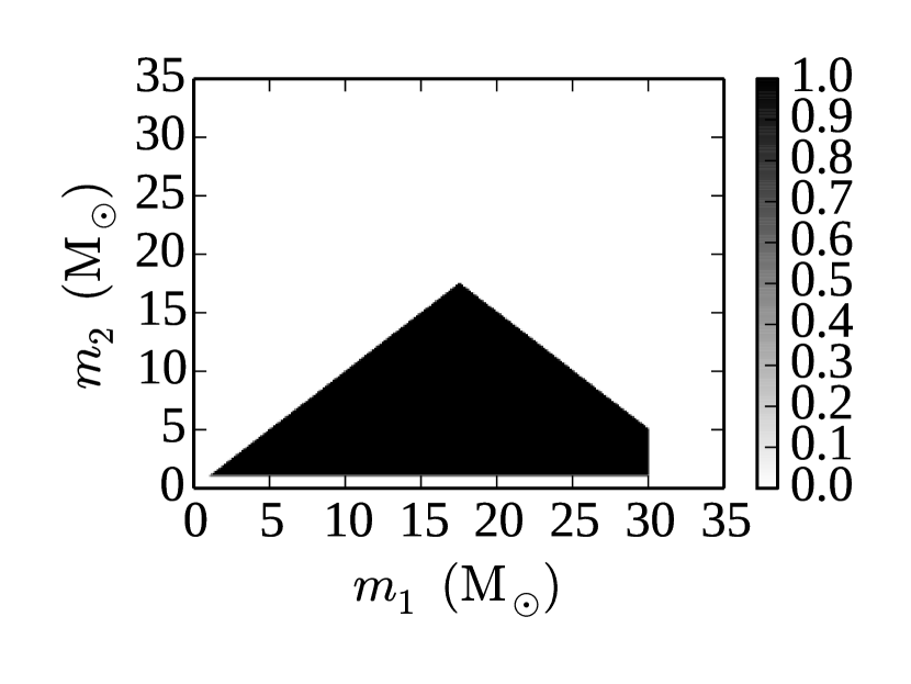
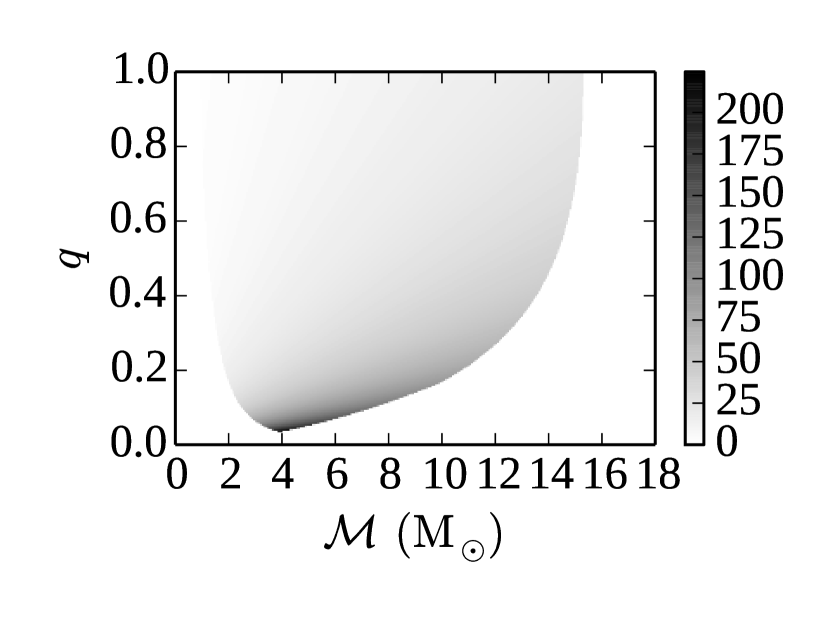
As shown in Eq. (1), the posterior distribution of $\theta$ (or $\bm{\theta}$) depends both on the likelihood and prior distributions of $\theta$. LALInference allows for flexibility in the choice of priors. For all analyses described here, we used the same prior density functions (and range). For component masses, we used uniform priors in the component masses with the range $1\,\mathrm{M}_{\odot}\leq m_{1,2}\leq 30\,\mathrm{M}_{\odot}$, and with the total mass constrained by $m_{1}+m_{2}\leq 35\,\mathrm{M}_{\odot}$, as shown in Fig. 1. This range encompasses the low-mass search range used in Abadie et al. (2012) and our previous parameter estimation report Aasi et al. (2013), where $1\,\mathrm{M}_{\odot}\leq m_{1,2}\leq 24\,\mathrm{M}_{\odot}$ and $m_{1}+m_{2}\leq 25\,\mathrm{M}_{\odot}$. When expressed in the sampling variable $\mathcal{M},q$ the prior is determined by the Jacobian of the transformation,

$$p(\mathcal{M},q|I)\propto\mathcal{M}m_{1}^{-2}$$ (21)

which is shown in the right panel of figure 1.

The prior density function on the location of the source was taken to be isotropically distributed on the sphere of the sky, with $p(d_{L}|H_{S})\propto{d_{L}}^{2}$, from $1$ Mpc out to a maximum distance chosen according to the detector configuration and the source type of interest. We used an isotropic prior on the orientation of the binary to give $p(\iota,\psi,\phi_{c}|H_{S})\propto\sin\iota$. For analyses using waveform models that account for possible spins, the prior on the spin magnitudes, $a_{1},a_{2}$, was taken to be uniform in the range $[0,1]$ (range $[-1,1]$ in the spin-aligned cases), and the spin angular momentum vectors were taken to be isotropic.

The computational cost of the parameter estimation pipeline precludes us from running it on all data; therefore, the parameter estimation analysis relies on an estimate of the coalescence time as provided by the detection pipeline Abadie et al. (2012). In practice, a 200 ms window centered on the trigger time is sufficient to guard against the uncertainty and bias in the coalescence time estimates from the detection pipeline, see for instance Brown (2004); Babak et al. (2013). For the signal-to-noise ratios (SNRs) used in this paper, our posteriors are much narrower than our priors for most parameters.

III Algorithms

III.1 MCMC

Markov chain Monte Carlo methods are designed to estimate a posterior by stochastically wandering through the parameter space, distributing samples proportionally to the density of the target posterior distribution. Our MCMC implementation uses the Metropolis–Hastings algorithm (Metropolis et al., 1953; Hastings, 1970), which requires a proposal density function $Q(\bm{\theta}^{\prime}|\bm{\theta})$ to generate a new sample $\bm{\theta}^{\prime}$, which can only depend on the current sample $\bm{\theta}$. Such a proposal is accepted with a probability $r_{s}=\text{min}(1,\alpha)$, where

$$\alpha=\frac{Q(\bm{\theta}|\bm{\theta}^{\prime})p(\bm{\theta}^{\prime}|\bm{d},H)}{Q(\bm{\theta}^{\prime}|\bm{\theta})p(\bm{\theta}|\bm{d},H)}\;.$$ (22)

If accepted, $\bm{\theta}^{\prime}$ is added to the chain, otherwise $\bm{\theta}$ is repeated.

Chains are typically started at a random location in parameter space, requiring some number of iterations before dependence on this location is lost. Samples from this burn-in period are not guaranteed to be draws from the posterior, and are discarded when estimating the posterior. Furthermore, adjacent samples in the chain are typically correlated, which is undesirable as we perform Kolmogorov-Smirnov tests of the sampled distributions, which requires independent samples. To remove this correlation we thin each chain by its integrated autocorrelation time (ACT) $\tau$, defined defined as

$$\tau =1+2\sum_{t}\hat{c}(t),$$ (23)

where $t$ labels iterations of the chain and $\hat{c}(t)$ is the Pearson correlation coefficient between the chain of samples and itself shifted by $t$ samples Gelman et al. (1996) The chain is thinned by using only every $\tau$-th sample, and the samples remaining after burn-in and ACT thinning are referred to as the effective samples. This is necessary for some post-processing checks which assume that the samples are statistically independent.

The efficiency of the Metropolis–Hastings algorithm is largely dependent on the choice of proposal density, since that is what governs the acceptance rates and ACTs. The standard, generically applicable distribution is a Gaussian centered on $\bm{\theta}$, the width of which will affect the acceptance rate of the proposal. Large widths relative to the scale of the target posterior distribution will lead to low acceptance rates with many repeated samples, whereas small widths will have high acceptance rates with highly correlated samples, both resulting in large ACTs. For a simplified setting of a unimodal Gaussian posterior, the optimal acceptance rate can be shown to be  $0.234$ Roberts and Rosenthal (1998). Though our posterior can be more complicated, we find that targeting this acceptance rate gives good performance and consistent ACTs for all posteriors that we have considered. Therefore, during the first 100,000 samples of a run, we adjust the 1D Gaussian proposal widths to achieve this acceptance rate. This period of adjustment is re-entered whenever the sampler finds a log likelihood ($\log L$) that is $N/2$ larger than has been seen before in a run, under the assumption that this increase in likelihood may indicate that a new area of parameter space is being explored.

When the posterior deviates from a unimodal Gaussian-like distribution, using only the local Gaussian proposal becomes very inefficient. The posteriors encountered in GW data analysis typically consists of multiple isolated modes, separated by regions of lower probability. To properly weigh these modes, a Markov chain must jump between them frequently, which is a very unlikely process when using only a local Gaussian proposal. In section III.3 we describe the range of jump proposals more adept at sampling the parameter space of a compact binary inspiral. We also describe the technique of parallel tempering, which we employ to ensure proper mixing of samples between the modes.

III.1.1 Parallel Tempering

Tempering Gilks et al. (1996); Earl and Deem (2005) introduces an inverse “temperature” $1/T$ to the standard likelihood function, resulting in a modified posterior

$$p_{T}(\bm{\theta}|\bm{d})\propto p(\bm{\theta}|H)L(\bm{\theta})^{\frac{1}{T}}\;.$$ (24)

Increasing temperatures above $T=1$ reduces the contrast of the likelihood surface, broadening peaks, with the posterior approaching the prior in the high temperature limit. Parallel tempering exploits this “flattening” of the posterior with increasing temperature by constructing an ensemble of tempered chains with temperatures spanning $T=1$ to some finite maximum temperature $T_{\text{max}}$. Chains at higher temperatures sample a distribution closer to the prior, and are more likely to explore parameter space and move between isolated modes. Regions of high posterior support found by the high-temperature chains are then passed down through the temperature ensemble by periodically proposing swaps in the locations of adjacent chains. Such swaps are accepted at a rate $r_{s}=\text{min}(1,\omega_{ij})$, where

$$\omega_{ij}=\left(\frac{L(\bm{\theta}_{j})}{L(\bm{\theta}_{i})}\right)^{\frac{1}{T_{i}}-\frac{1}{T_{j}}}\;,$$ (25)

with $T_{i}<T_{j}$.

For non-trivial posteriors this technique greatly increases the sampling efficiency of the $T=1$ chain, but does so at a cost. In our implementation, samples with $T>1$ are not used in construction of the final posterior distribution, but they are kept for calculation of evidence integrals via thermodynamic integration in post-processing IV.3.

All samples from chains with $T>1$ are ultimately discarded, as they are not drawn from the target posterior. From a computational perspective however, each chain can run in parallel and not affect the total run time of the analysis. The MCMC implementation of LALInference, LALInferenceMCMC, uses the Message Passing Interface (MPI) Forum (1994) to achieve this parallelization. In our calculations, the temperatures $T_{i}$ are distributed logarithmically. Chains are not forced to be in sync, and each chain proposes a swap in location with the chain above it (if one exists) every 100 samples.

III.2 Nested Sampling

Nested sampling is a Monte Carlo technique introduced by Skilling Skilling (2006) for the computation of the Bayesian evidence that will also provide samples from the posterior distribution. This is done by transforming the multi-dimensional integral of Equation (4) into a one-dimensional integral over the prior volume. The prior volume is defined as $X$ such that $\mathrm{d}X=\mathrm{d}\bm{\theta}p(\bm{\theta}|H)$. Therefore,

$$X(\lambda)=\int_{p(d|\bm{\theta},H)>\lambda}\mathrm{d}\bm{\theta}p(\bm{\theta}|H).$$ (26)

This integral computes the total probability volume contained within a likelihood contour defined by $p(d|\bm{\theta},H)=\lambda$. With this in hand, Equation (4) can now be written as

$$Z=\int_{0}^{1}L(X)\mathrm{d}X,$$ (27)

where $L(X)$ is the inverse of Equation (26) and is a monotonically decreasing function of $X$ (larger prior volume enclosed implies lower likelihood value). By evaluating the likelihoods $L_{i}=L(X_{i})$ associated with a monotonically decreasing sequence of prior volumes $X_{i}$,

$$0<X_{M}<\ldots<X_{2}<X_{1}<X_{0}=1,$$ (28)

the evidence can be easily approximated with the trapezium rule,

$$Z=\sum_{i=1}^{M}\frac{1}{2}(X_{i-1}-X_{i+1})L_{i}.$$ (29)

Examples of the function $L(X)$ for CBC sources are shown in figure 2.

Figure 2: The profile of the likelihood function for each of the injections in Table 2, mapped onto the fractional prior support parameter $X$ (see Eq. (28)). The algorithm proceeds from left (sampling entire prior) to right (sampling a tiny restricted part of the prior). The values of $\log(L)$ are normalised to the likelihood of the noise model.

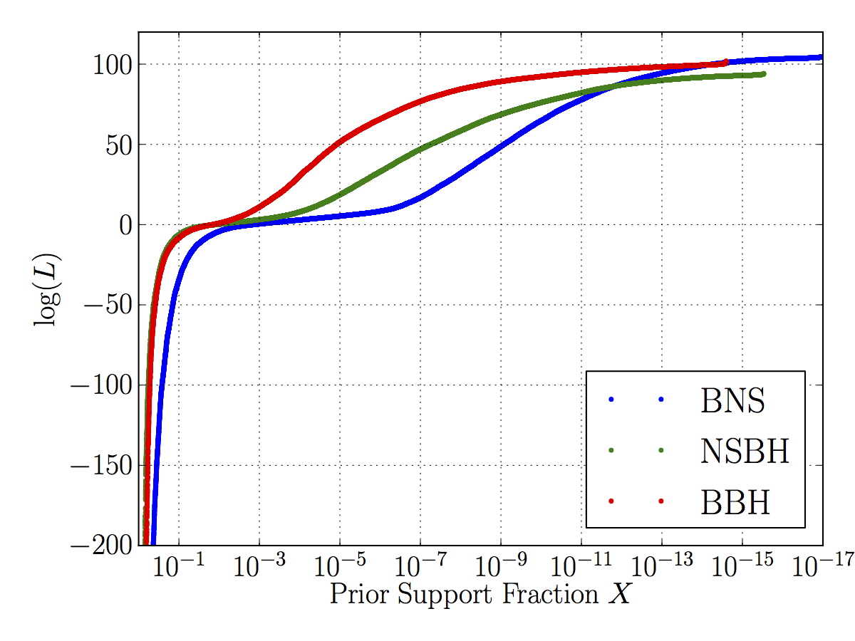
Applying this technique follows a fundamental set of steps. First, a set of initial ‘live’ points are sampled from the entire prior distribution. The point with the lowest likelihood value is then removed and replaced by a new sample with higher likelihood. This removal and replacement is repeated until a stopping condition has been reached. By default, the loop continues while $L_{max}X_{i}/Z_{i}>e^{0.1}$, where $L_{max}$ is the maximum likelihood so far discovered by the sampler, $Z_{i}$ is the current estimate of the total evidence, and $X_{i}$ is the fraction of the prior volume inside the current contour line. In short, this is checking whether the evidence estimate would change by more than a factor of $\sim 0.1$ if all the remaining prior support were at the maximum likelihood. Posterior samples can then be produced by re-sampling the chain of removed points and current live points according to their posterior probabilities:

$$p(\bm{\theta}|d,H)=\frac{\tfrac{1}{2}(X_{i-1}-X_{i+1})L_{i}}{Z}.$$ (30)

The estimation of the prior volume and method for efficiently generating new samples varies between implementations. In LALInference we have included two such implementations, one based on an MCMC sampling of the constrained prior distribution, and the other on the MultiNest method, with extensions. These are described in the following two sections III.2.1 and III.2.2.

III.2.1 LALInferenceNest

The primary challenge in implementing the nested sampling algorithm is finding an efficient means of drawing samples from the limited prior distribution

$$p^{\prime}(\bm{\theta}|H_{S})\propto\begin{cases}p(\bm{\theta}|H_{S})&\quad L(\bm{d}|\bm{\theta})>L_{\rm min}\\ 0&\quad\text{otherwise}\end{cases}.$$ (31)

In LALInference we build on the previous inspnest implementation described in Veitch and Vecchio (2010), with several enhancements described here. This uses a short MCMC chain (see section III.1) to generate each new live point, which is started from a randomly-selected existing live point.

We use proposals of the same form as described in III.3 with slight differences: the differential evolution proposal is able to use the current set of live points as a basis for drawing a random difference vector, and for empirically estimating the correlation matrix used in the eigenvector proposal. This ensures that the scale of these jumps adapts automatically to the current concentration of the remaining live points. In contrast to Eq. (22), the target distribution that we are sampling is the limited prior distribution $p^{\prime}$ of Eq. (31), so the acceptance ratio is

$$\alpha =\frac{Q(\bm{\theta}|\bm{\theta}^{\prime})p^{\prime}(\bm{\theta}^{\prime}|H)}{Q(\bm{\theta}^{\prime}|\bm{\theta})p^{\prime}(\bm{\theta}|H)}.$$ (32)

Furthermore, we have introduced additional features which help to reduce the amount of manual tuning required to produce a reliable result.

Autocorrelation adaptation

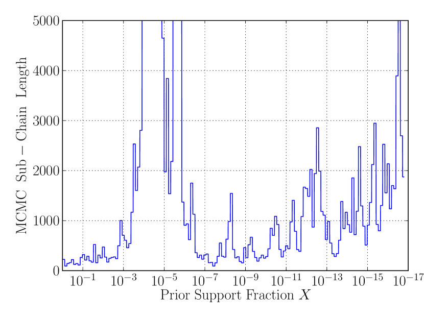
In Veitch and Vecchio (2010) it was shown that the numerical error on the evidence integral was dependent not only on the number of live points $N_{\rm live}$ and the information content of the data (as suggested by Skilling), but also on the length of the MCMC sub-chains $N_{\rm MCMC}$ used to produce new samples (this is not included in the idealised description of nested sampling, since other methods of drawing independent new samples are also possible, see section III.2.2). In inspnest, the user would specify this number at the start of the run, depending on their desire for speed or accuracy. The value then remained constant throughout the run. This is inefficient, as the difficulty of generating a new sample varies with the structure of the $p^{\prime}(\bm{\theta}|H_{S})$ distribution at different values of $L_{\rm min}$. For example, there may be many secondary peaks which are present up to a certain value of $L_{\rm min}$, but disappear above that, making the distribution easier to sample. To avoid this inefficiency (and to reduce the number of tuning parameters of the code), we now internally estimate the required length of the sub-chains as the run progresses. To achieve this, we use the estimate of the autocorrelation timescale $\tau_{i}$ (defined as in Eq. 23) for parameter $i$ of a sub-chain generated from a randomly selected live point. The sum is computed up to the lag $M_{i}$ which is the first time the correlation drops below $0.01$, i.e $\hat{c}_{i}(M_{i})\leq 0.01$. The timescale is computed for each parameter being varied in the model, and the longest autocorrelation time is used as the number of MCMC iterations ($M=\mathrm{max}(M_{1},\ldots,M_{i})$ for subsequent sub-chains until it is further updated after $N_{\rm live}/4$ iterations of the nested sampler. As the chain needed to compute the autocorrelation timescale is longer than the timescale itself, the independent samples produced are cached for later use. We note that as the nested sampling algorithm uses many live points, the correlation between subsequent points used for evaluating the evidence integral will be further diluted, so this procedure is a conservative estimate of the necessary chain thinning. The adaptation of the sub-chain length is shown in figure 3, where the algorithm adapts to use $<1000$ MCMC steps during the majority of the analysis, but can adjust its chain length to a limit of 5000 samples for the most difficult parts of the problem.

Figure 3: Length of MCMC sub-chain for nested sampling analysis of the BNS system (as in Table 2) as a function of prior scale. As the run progresses, the length of the MCMC sub-chain used to generate the next live point automatically adapts to the current conditions, allowing it to use fewer iterations where possible. The chain is limited to a maximum of 5000 iterations.

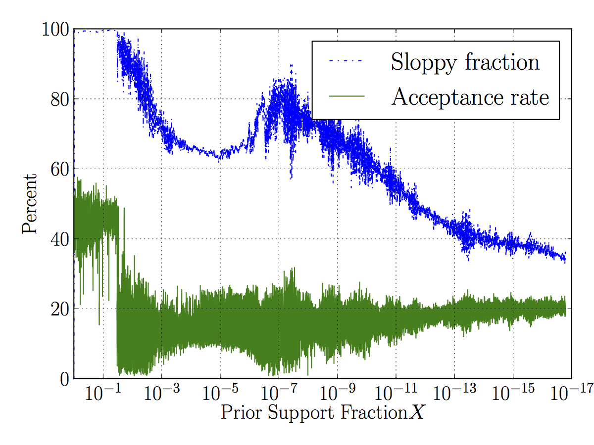
Sloppy sampling

For the analysis of CBC data, the computational cost of a likelihood evaluation completely dominates that of a prior calculation, since it requires the generation of a trial waveform and the calculation of an inner product (with possible FFT into the frequency domain). The task of sampling the likelihood-limited prior $p^{\prime}(\bm{\theta}|H)$ is performed by sampling from the prior distribution, rejecting any points that fall beneath the minimum threshold $L_{\rm min}$. During the early stages of the run, the $L_{\rm min}$ likelihood bound encloses a large volume of the parameter space, which may take many iterations of the sub-chain to cross, and a proposed step originating inside the bound is unlikely to be rejected by this cut. We are free to make a shortcut by not checking the likelihood bound at each step of the sub-chain, allowing it to continue for $ME$ iterations, where $E$ is the fraction of iterations where the likelihood check is skipped. Since the calculation of the prior is essentially free compared to that of the likelihood, the computational efficiency is improved by a factor of $~{}(1-E)^{-1}$. The likelihood bound is always checked before the sample is finally accepted as a new live point.

Since the optimal value of $E$ is unknown, and will vary throughout the run as the $L_{\rm min}$ contour shrinks the support for the $p^{\prime}(\bm{\theta}|H)$ distribution, we adaptively adjust it based on a target for the acceptance of proposals at the likelihood-cut stage. Setting a target acceptance rate of 0.3 at the likelihood cut stage, and having measured acceptance rate $\alpha$, we adjust $E$ in increments of $5\%$ upward when $\alpha>0.3$ or downward when $\alpha<0.3$, with a maximum of $1$. This procedure allows the code to calculate fewer likelihoods when the proposal distribution predominantly falls inside the bounds, which dramatically improves the efficiency at the start of the run.

Figure 4: Acceptance ratio and fraction of sloppy jumps for nested sampling analysis of a BNS system. The dashed blue line shows the automatically determined fraction of proposals for which the likelihood calculation is skipped. The solid green line shows the overall acceptance rate for new live points, which thanks to the adaptive jumps remains at a healthy level despite the volume of the sampled distribution changing by 17 orders of magnitude throughout the run.

Parallelisation

Although the nested sampling algorithm itself is a sequential method, we are able to exploit a crude parallelisation method to increase the number of posterior samples produced. This involves performing separate independent runs of the algorithm on different CPU cores, and then combining the results weighted by their respective evidence. Consider a set of nested sampling runs indexed by $i$, with each iteration indexed by $j=1\ldots\xi_{i}$, where $\xi_{i}$ is the number of iterations in run $i$ before it terminates, and $Z_{i}$ denotes the evidence estimate from that run. Our implementation also outputs the $N_{\mathrm{live}}$ live points at the time of algorithm termination, which are indexed $\xi_{i+1}\ldots\xi_{i+N_{\mathrm{live}}}$. These last samples are treated separately since they are all drawn from the same prior volume. The runs must all be performed with identical data and models, but with different random seeds for the sampler.

For each sample $\bm{\theta}_{ij}$ we calculate the posterior weight $w_{ij}=L_{ij}V_{ij}/Z_{i}$, where $\log V_{ij}=-j/N_{\mathrm{live}}$ for the points up to $j\leq\xi_{i}$ and $V_{ij}=-\xi_{i}/N_{\mathrm{live}}$ for the final points $j>\xi_{i}$. By resampling any individual chain according to the weights $w_{ij}$ we can produce a set of samples from the posterior. The resulting sets of posteriors for each $i$ are then resampled according to the evidence $Z_{i}$ calculated for each chain. This ensures that chains which fail to converge on the global maximum will contribute proportionally fewer samples to the final posterior than those which do converge and produce a higher $Z_{i}$ estimate. The resampling processes can be performed either with or without replacement, where the latter is useful in ensuring that no samples are repeated. In this paper independent samples are used throughout, as repeated samples will distort the tests of convergence by artificially lowering the KS test statistic.

In practice, this procedure reduces the wall time necessary to produce a given number of posterior samples, as the chains can be spread over many CPU cores.

III.2.2 MultiNest & BAMBI

MultiNest Feroz and Hobson (2008); Feroz et al. (2009, 2013) is a generic algorithm that implements the nested sampling technique. It uses a model-based approach to generate samples within the volume $X$ enclosed by the likelihood contour $L(X)>L_{\mathrm{min}}$. The set of live points is enclosed within a set of (possibly overlapping) ellipsoids and a new point is then drawn uniformly from the region enclosed by these ellipsoids. The volume of ellipsoids is used in choosing which to sample from and points are tested to ensure that if they lie in multiple ($N$) ellipsoids they are accepted as a sample only the corresponding fraction of the time ($1/N$). The ellipsoidal decomposition of the live point set is chosen to minimize the sum of volumes of the ellipsoids. This method is well suited to dealing with posteriors that have curving degeneracies, and allows mode identification in multi-modal posteriors. If there are various subsets of the ellipsoid set that do not overlap in parameter space, these are identified as distinct modes and subsequently evolved independently.

MultiNest is able to take advantage of parallel computing architectures by allowing each CPU to compute a new proposal point. As the run progresses, the actual sampling efficiency (fraction of accepted samples from total samples proposed) will drop as the ellipsoidal approximation is less exact and the likelihood constraint on the prior is harder to meet. By computing $N$ samples concurrently, we can obtain speed increases of up to a factor of $N$ with the largest increase coming when the efficiency drops below $1/N$.

The user only needs to tune a few parameters for any specific implementation in addition to providing the log-likelihood and prior functions. These are the number of live points, the target efficiency, and the tolerance. The number of live points needs to be enough that all posterior modes are sampled (ideally with at least one live point in the initial set) and we use from $1000$ to $5000$ for our analyses. The target efficiency affects how conservatively the ellipsoidal decomposition is made and a value of $0.1$ ($10\%$) was found to be sufficient; smaller values will produce more precise posteriors but require more samples. Lastly, a tolerance of $0.5$ in the evidence calculation is sufficiently small for the run to converge to the correct result.

MultiNest is implemented for LALInference within the Blind Accelerated Multimodal Bayesian Inference (BAMBI) algorithm Graff et al. (2012). BAMBI incorporates the nested sampling performed by MultiNest along with the machine learning of SkyNet Graff et al. (2014) to learn the likelihood function on-the-fly. Use of the machine learning capability requires further customisation of input settings and so is not used for the purposes of this study.

III.3 Jump Proposals

For both the MCMC sampler and the MCMC-subchains of the Nested Sampler, efficiently exploring the parameter space is essential to optimising performance of the algorithms. Gaussian jump proposals are typically sufficient for unimodal posteriors and spaces without strong correlations between parameters, but there are many situations where strong parameter correlations exist and/or multiple isolated modes appear spread across the multi-dimensional parameter space. When parameters are strongly correlated, the ideal jumps would be along these correlations, which makes 1D jumps in the model parameters very inefficient. Furthermore to sample between isolated modes, a chain must make a large number of improbable jumps through regions of low probability. To solve this problem we have used a range of jump proposals, some of which are specific to the CBC parameter estimation problem and some of which are more generally applicable to multimodal or correlated problems.

To ensure that an MCMC equilibrates to the target distribution, the jump proposal densities in Eq. (22) must be computed correctly. Our codes achieve this using a “proposal cycle.” At the beginning of a sampling run, the proposals below are placed into an array (each proposal may be put multiple times in the array, according to a pre-specified weight factor). The order of the array is then permuted randomly before sampling begins. Throughout the run, we cycle through the array of proposals (maintaining the order), computing and applying the jump proposal density for the chosen proposal at each step as in Eq. (22). This procedure ensures that there is only a single proposal “operating” for each MCMC step, simplifying the computation of the jump proposal density, which otherwise would have to take into account the forward and reverse jump probabilities for all the proposals simultaneously.

Differential Evolution

Differential evolution is a generic technique that attempts to solve the multimodal sampling problem by leveraging information gained previously in the run (ter Braak, 2006; ter Braak and Vrugt, 2008). It does so by drawing two previous samples $\bm{\theta}_{1}$ and $\bm{\theta}_{2}$ from the chain (for MCMC) or from the current set of live points (nested sampling), and proposing a new sample $\bm{\theta}^{\prime}$ according to:

$$\bm{\theta}^{\prime}=\bm{\theta}+\gamma(\bm{\theta}_{2}-\bm{\theta}_{1})\;,$$ (33)

where $\gamma$ is a free coefficient. 50% of the time we use this as a mode-hopping proposal, with $\gamma=1$. In the case where $\bm{\theta}_{1}$ and $\bm{\theta}$ are in the same mode, this proposes a sample from the mode containing $\bm{\theta}_{2}$. The other 50% of the time we choose $\gamma$ according to

$$\gamma\sim N\left(0,2.38/\sqrt{2N_{\mathrm{dim}}}\right),$$ (34)

where $N_{\mathrm{dim}}$ is the number of parameter space dimensions. The scaling of the distribution for $\gamma$ is suggested in ter Braak and Vrugt (2008) following Roberts and Rosenthal (2001) for a good acceptance rate with general distributions. The differential evolution proposal in this latter mode proves useful when linear correlations are encountered in the distribution, since the jump directions tend to lie along the principal axes of the posterior distribution. However, this proposal can perform poorly when the posterior is more complicated.

Drawing from the past history of the chain for the MCMC differential evolution proposal makes the chain evolution formally non-Markovian. However, as more and more points are accumulated in the past history, each additional point accumulated makes a smaller change to the overall proposal distribution. This property is sufficient to make the MCMC chain asymptotically Markovian, so the distribution of samples converges to the target distribution; in the language of Roberts and Rosenthal (2007), Theorem 1, $D_{n}\to 0$ in probability as $n\to\infty$ for this adaptive proposal, and therefore the posterior is the equilibrium distribution of this sampling.

Eigenvector jump

The variance-covariance matrix of a collection of representative points drawn from the target distribution (the current set of nested sampling live points) can be used as an automatically self-adjusting proposal distribution. In our implementation, we calculate the eigenvalues and eigenvectors of the estimated covariance matrix, and use these to set a scale and direction for a jump proposal. This type of jump results in a very good acceptance rate when the underlying distribution is approximately Gaussian, or is very diffuse (as in the early stages of the nested sampling run). In the nested sampling algorithm, the covariance matrix is updated every $N_{live}/4$ iterations to ensure the jump scales track the shrinking scale of the target distribution. Within each sub-chain the matrix is held constant to ensure detailed balance.

Adaptive Gaussian

We also use a 1 dimensional Gaussian jump proposal, where the jump for a single parameter $\theta_{k}$ is $\theta_{k}^{\prime}=\theta_{k}+N(0,\sigma_{k})$. The width of the proposal is scaled to achieve a target acceptance rate of $\xi\simeq 0.234$ by adjusting

$$\sigma_{k}\leftarrow\sigma_{k}+s_{\gamma}\frac{1-\xi}{100}\Delta$$ (35)

when a step is accepted, where $s_{\gamma}$ is a scaling factor and $\Delta$ is the prior width in the $k$th parameter, and adjusting

$$\sigma_{k}\leftarrow\sigma_{k}-s_{\gamma}\frac{\xi}{100}\Delta$$ (36)

when a step is rejected. For the MCMC, the adaptation phase lasts for 100,000 samples, and $s_{\gamma}=10\left(t-t_{0}\right)^{-1/5}-1$ during this phase; otherwise $s_{\gamma}=0$. The nested sampling algorithm has $s_{\gamma}=1$.

Gravitational-wave specific proposals

We also use a set of jump proposals specific to the CBC parameter estimation problem addressed in this work. These proposals are designed to further improve the sampling efficiency by exploring known structures in the CBC posterior distribution, primarily in the sky location and extrinsic parameter sub-spaces.

Sky location

Determining the sky position of the CBC source is an important issue for followup observations of any detected sources. The position, parameterised by $(\alpha,\delta,d_{L})$, is determined along with the other parameters by the LALInference code, but it can present difficulties due to the highly structured nature of the posterior distribution. Although the non-uniform amplitude response of a single detector allows some constraint of the sky position of a source, the use of a network of detectors gives far better resolution of the posterior distribution. This improvement is heuristically due to the ability to resolve the difference in time of arrival of the signal at each detector, which allows triangulation of the source direction. The measured amplitude of the signal and the non-uniform prior distribution further constrain the posterior, but the major structure in the likelihood can be derived by considering the times of arrival in multiple detectors. This leads us to include two specific jump proposals similar to those outlined in Veitch and Vecchio (2010), which preserve the times of arrival in two and three detector networks respectively.

Sky Reflection

In the case of a three-detector network, the degeneracy of the ring based on timing is broken by the presence of a third detector. In this case, there are two solutions to the triangulation problem which correspond to the true source location, and its reflection in the plane containing the three detector sites. If the normal vector to this plane is $\hat{n}$, the transition (in Cartesian coordinates with origin at the geocentre) between the true point $\hat{x}$ and its reflection $\hat{x}^{\prime}$ is written

$$\hat{x}^{\prime}=\hat{x}-2\hat{n}|\hat{n}.(\hat{x}-\hat{x}_{i})|$$ (37)

where $\hat{x}_{i}$ is the unit vector pointing in the direction of one of the detector sites. The resulting point is then projected back onto the unit sphere parameterised by $\alpha,\delta$. To ensure detailed balance, the resulting point is perturbed by a small random vector drawn from a 3D Gaussian in $(t,\alpha,\delta)$ The time parameter is updated in the same way as for the sky rotation proposal above. As in the two-detector case, the degeneracy between these points can be broken by consideration of the signal amplitudes observed in the detector, however this is not always the case as the secondary mode can have a similar likelihood.

Extrinsic parameter proposals

Extrinsic Parameter proposal

There exist a correlation between the inclination, distance, polarization and the sky location dues to the sensitivity of the antenna beam patterns of the detectors. This correlation makes the two solutions for the sky location from the thee-detector network (described above) correspond to different values of inclination, distance and polarization. We solve analytically the values of those parameters when trying to jump between the two sky reflections. The equations are detailed in Raymond and Farr (2014).

Polarization and Phase correlation

There exists a degeneracy between the $\phi$ and $\psi$ parameters when the orbital plane is oriented perpendicular to the line of signal, i.e. $\iota=\{0,\pi\}$. In general these parameters tend to be correlated along the axes $\alpha=\psi+\phi$ and $\beta=\psi-\phi$. We propose jumps which choose a random value of either the $\alpha$ or $\beta$ parameter (keeping the other constant) to improve the sampling of this correlation.

Miscellaneous proposals

Draw from Prior

A proposal that generates samples from the prior distribution (see section II.3) by rejection sampling. This is mostly useful for improving the mixing of high-temperature MCMC chains, as it does not depend on the previous iteration.

Phase reversal

Proposes a change in the orbital phase parameter $\phi_{j+1}=(\phi_{j}+\pi)\pmod{2\pi}$, which will keep the even harmonics of the signal unchanged, but will flip the sign of the odd harmonics. Since the even harmonic $l=m=2$ dominates the signal, this is useful for proposing jumps between multiple modes which differ only by the relatively small differences in the waveform generated by the odd harmonics.

Phase and polarization reversal

Proposes a simultaneous change of the orbital phase and polarisation parameters $\phi_{j+1}=(\phi_{j}+\pi)\,\pmod{2\pi}$ and $\psi_{j+1}=(\psi_{j}+\pi/2)\,\pmod{\pi}$.

Gibbs Sampling of Distance

The conditional likelihood of the distance parameter $d_{L}$ follows a known form, which allows us to generate proposals from this distribution independently of the previous iteration, reducing the correlation in the chains. As the signal amplitude scales proportionally to ${d_{L}}^{-1}=u$, the logarithm of the likelihood function (Equation (10)), constrained to only distance variations, is quadratic in $u$,

$$\log L(u) =A+Bu+Cu^{2},$$ (38)

which in our case yields a Gaussian distribution with mean $\mu=-B/2C$ and variance $\sigma^{2}=1/2C$. By calculating the value of $\log L$ at three different distances, the quadratic coefficients are found and a new proposed distance can be generated from the resulting Gaussian distribution.

IV Post-processing

The main data products of all the above algorithms are a set of ‘samples’ assumed to be drawn independently from the posterior probability distribution $p(\bm{\theta}|d,I)$ (as defined in Equation (1)) and, for the nested sampling algorithms, an approximation to the evidence $Z=P(d|I)$ (for MCMC, evidence computation is performed in post-processing, see section IV.3). Each algorithm initially produces outputs which are different in both their form and relation to these quantities. A suite of Python scripts has been specifically developed for the purpose of converting these outputs to a common results format in order to facilitate comparisons between the algorithms and promote consistency in the interpretation of results. At the time of writing these scripts (and associated libraries) can be found in the open-source LALsuite package LAL . The end result of this process is a set of web-ready HTML pages containing the key meta-data and statistics from the analyses and from which it should be possible to reproduce any results produced by the codes. In this section we outline in more detail the steps needed to convert or post-process the output of the different algorithms to this common results format and important issues related to interpreting these results and drawing scientific conclusions.

IV.1 MCMC

The MCMC algorithm in LALInference produces a sequence of $O(10^{6})$ - $O(10^{8})$ samples, depending on the number of source parameters in the model, the number of interferometers used, and the bandwidth of the signal. Each sample consists of a set of source parameters $\{\bm{\theta}\}$ and associated values of the likelihood function $L(d|\bm{\theta})$ and prior $p(\bm{\theta})$. We cannot immediately take this output sequence to be our posterior samples as we cannot assume that all the samples were drawn independently from the actual posterior distribution.

In order to generate a set of independent posterior samples the post-processing for the MCMC algorithm first removes a number of samples at the beginning of the chain – the so-called ‘burn-in’ – where the MCMC will not yet be sampling from the posterior probability density function. For a $d$-dimensional parameter space, the distribution of the log-likelihood is expected to be close to $\mathcal{L}_{\text{max}}-X$, where $\mathcal{L}_{\text{max}}$ is the maximum achievable log-likelihood, and $X$ is a random variable following a Gamma($d/2$, 1) distribution Raftery et al. (2007). Thus, we consider the burn-in to end when a chain samples log-likelihood values that are within $d/2$ of the highest log-likelihood value found by the chain. Once we have discarded these samples, the set of remaining samples is then ‘down-sampled’; the chain is re-sampled randomly at intervals inversely proportional to the the autocorrelation length to produce a sub-set of samples which are assumed to be drawn independently from the posterior distribution. See section III.1 above for more details.

IV.2 Nested sampling

The output of both of the nested sampling algorithms in LALInference are a list (or lists in the case of parallel runs) of the live points sampled from the prior distribution for a particular model and data set and consisting of a set of parameters and their associated $\log(L_{ij})$ and $Z_{ij}$. These live points approximately lie on the contours enclosing the nested prior volumes and each has associated with it some fraction of the evidence assumed to be enclosed within said contour. The post-processing step takes this information and uses it to generate posterior samples from the list of retained live points using Eq. 30 for single runs, along with the procedure described in section III.2.1 for parallel runs.

IV.3 Evidence calculation using MCMC outputs

Whilst the nested sampling algorithms in LALInference directly produce an approximation to the value of the evidence $Z$ (and produce posterior samples as a by-product), we can also use the output from the MCMC algorithms to calculate independent estimates of $Z$ in post-processing. We have tested several methods of computing the evidence from posterior samples, including the harmonic mean (Newton and Raftery, 1994; Chib, 1995; van Haasteren, 2009), direct integration of an estimate of the posterior density (Weinberg, 2009), and thermodynamic integration (see e.g. R. M. Neal (1993); Littenberg and Cornish (2009)). We have found that only thermodynamic integration permits reliable estimation of the evidence for the typical number and distribution of posterior samples we obtain in our analyses.

Thermodynamic integration considers the evidence as a function of the temperature, $Z(\beta|H)$, defined as

$$Z(\beta|H) \equiv\int\mathrm{d}\bm{\theta}p(d|H,\bm{\theta},\beta)p(\bm{\theta}|H)$$

$$=\int\mathrm{d}\bm{\theta}p(d|H,\bm{\theta})^{\beta}p(\bm{\theta}|H)$$ (39)

where $\beta=1/T$ is the inverse temperature of the chain. Differentiating with respect to $\beta$, we find

$$\frac{d}{\mathrm{d}\beta}\ln Z(\beta|H)=\langle\ln p(d|H,\bm{\theta})\rangle_{\beta}$$ (40)

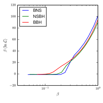
where $\langle\ln p(d|H,\bm{\theta})\rangle_{\beta}$ is the expectation value of the log likelihood for the chain with temperature $1/\beta$. We can now integrate (40) to find the logarithm of the evidence

$$\ln Z=\int_{0}^{1}\mathrm{d}\beta\ \langle\ln p(d|H,\bm{\theta})\rangle_{\beta}.$$ (41)

It is straightforward to compute $\langle\ln p(d|H,\bm{\theta})\rangle_{\beta}$ for each chain in a parallel-tempered analysis; the integral in Eq. (41) can then be estimated using a quadrature rule. Because our typical temperature spacings are coarse, the uncertainty in this estimate of the evidence is typically dominated by discretisation error in the quadrature. We estimate that error by performing the quadrature twice, once using all the temperatures in the chain and once using half the temperatures. To achieve very accurate estimates of the evidence, sometimes $\sim 20$ to $\sim 30$ temperatures are needed, out to a maximum of $\beta^{-1}\sim 10^{5}$, which adds a significant cost over the computations necessary for parameter estimation; however, reasonably accurate estimates of the evidence can nearly always be obtained from a standard run setup with $\sim 10$ chains. Figure 5 plots the integrand of Eq. (41) for the synthetic GW signals analysed in § V.2, illustrating both the coarse temperature spacing of the runs and the convergence of the evidence integral at high temperature.

Figure 5: The integrand of the evidence integral (Eq. (41)) versus $\beta$ for the analyses of synthetic GW signals in § V.2. The evidence is given by the area under each curve. Table 1 gives the results of the integration together with the estimated error in the quadrature, following the procedure described in § IV.3. The jaggedness of the curves illustrates that the temperature spacing required for convergent MCMC simulations is larger than that required for accurate quadrature to compute the evidence; the flatness at small $\beta$ illustrates that, for these simulations, the high-temperature limit is sufficient for convergence of the evidence integral.

IV.4 Generation of statistics and marginal posterior distributions

Whilst the list of posterior samples contains all the information about the distribution of the source parameters obtained from the analysis, we need to make this more intelligible by summarising it in an approximate way. We have developed a number of different summary statistics which provide digested information about the posterior distributions, which are applied in post-processing to the output samples.

The simplest of these are simply the mean and standard deviation of the one-dimensional marginal distributions for each of the parameters. These are estimated as the sample mean, standard deviation, etc., over the samples, which converge on their continuous distribution equivalents (3) in the limit of large numbers of samples. These are particularly useful for giving simple measures of the compatibility of the results with the true values, if analysing a known injection.

However, estimators are not always representative of the much larger amount of information contained in the marginal posterior distributions on each of the parameters (or combinations of them). For summarising one- or two-dimensional results we create plots of the marginal posterior probability density function by binning the samples in the space of the parameters and normalising the resulting histogram by the number of samples.

We are also interested in obtaining estimates of the precision of the resulting inferences, especially when comparing results from a large number of simulations to obtain an expectation of parameter estimation performance under various circumstances. We quantify the precision in terms of ‘credible intervals’, defined for a desired level of credibility (e.g. $P_{\mathrm{cred}}=95\%$ probability that the parameter lies within the interval), with the relation

$$\mathrm{credible\phantom{a}level}=\int_{\mathrm{credible\phantom{a}interval}}p(\bm{\theta}|d)d\bm{\theta}.$$ (42)

The support of the integral above is the credible interval, however this is not defined uniquely by this expression. In one dimension, we can easily find a region enclosing a fraction $x$ of the probability by sorting the samples by their parameter values and choosing the range from $[N(1-x)/2,N(1+x)/2]$ where $N$ is the number of independent samples in the posterior distribution. The statistical error on the fraction $x$ of the true distribution enclosed, caused by the approximation with discrete samples is $\approx\sqrt{x(1-x)/N}$. To achieve a $1\%$ error in the $90\%$ region we therefore require 900 independent samples. Typically we collect a few thousand samples, giving an error $<1\%$ on the credible interval.

We are also interested in the minimum credible interval, which is the smallest such region that encloses the desired fraction of the posterior. In the case of a unimodal one-dimensional posterior this leads to the highest posterior density interval.

To find estimates of the minimum credible intervals we use a number of techniques that have different regimes of usefulness, depending primarily on the number of samples output from the code and the number of parameters we are interested in analysing conjointly.

When we are considering the one-dimensional marginal posterior distributions, we simply compute a histogram for the parameter of interest using equally-sized bins. This directly tells us the probability associated with that region of the parameter space: the probability density is approximately equal to the fraction of samples in the bin divided by the bin width. This simple histogram method involves an appropriate choice of the bin size. We must be careful to choose a bin size small enough that we have good resolution and can approximate the density as piecewise constant within each bin, but large enough so that the sampling error within each bin does not overwhelm the actual variations in probability between bins.

To recover the minimum credible interval we apply a greedy algorithm to the histogram bins. This orders the bins by probability, and starting from the highest probability bin, works its way down the list of bins until the required total probability has been reached. Although this procedure generally yields satisfactory results, it is subject to bias due to the discrete number of samples per bin. To see this, consider a uniform probability distribution that has been discretely sampled. The statistical variation of the number of samples within bins will cause those where the number fluctuates upward to be chosen before those where it fluctuates downward. The credible interval estimated by this method will therefore be smaller than the true interval containing the desired proportion of the probability. In Sidery et al. (2014) we investigate several methods of overcoming this problem.

V Validation of results

To confirm the correctness of the sampling algorithms, we performed cross-comparisons of recovered posterior distributions for a variety of known distributions and example signals. The simplest check we performed was recovery of the prior distribution, described in section II.3. The one-dimensional distributions output by the codes were compared using a Kolmogorov-Smirnov test, where the comparisons between the three codes on the 15 marginal distributions were all in agreement with p-values above $0.02$. We next analysed several known likelihood functions, where we could perform cross-checks between the samplers. These were a unimodal $15$-dimensional correlated Gaussian, a bimodal correlated Gaussian distribution, and the Rosenbrock banana function. For the unimodal and bimodal distributions we can also compare the results of the samplers to the analytical marginal distributions to confirm they are being sampled correctly.

V.1 Analytic likelihoods

		Nested		MCMC
Distribution	Analytic	Sampling	BAMBI	thermo.
Unimodal	-21.9	$-21.8\pm 0.1$	$-21.8\pm 0.12$	$-20.3\pm 1.9$
Bimodal	-30.0	$-30.0\pm 0.1$	$-29.9\pm 0.14$	$-26.7\pm 3.0$
Rosenbrock	–	$-70.9\pm 0.2$	$-69.1\pm 0.2$	$-63.0\pm 7.6$
BNS	–	$68.7\pm 0.34$	$69.98\pm 0.17$	$68.2\pm 1.1$
NSBH	–	$62.2\pm 0.27$	$63.67\pm 0.16$	$63.40\pm 0.72$
BBH	–	$71.4\pm 0.18$	$72.87\pm 0.15$	$72.44\pm 0.11$

Table 1: The log evidence estimates for the analytic likelihood distributions (§V.1) and the simulated signals (§V.2) calculated with the three methods, with estimated uncertainty. For the thermodynamic integration method we used 16 steps on the temperature ladder, except for the Rosenbrock likelihood which required 64. For distributions that permit an analytic computation of evidence, the samplers produce evidence estimates consistent with the true value. For the others, the estimates produced by the samplers are not consistent, indicating that there remains some systematic error in the evidence calculation methods for the more difficult problems.

The multivariate Gaussian distribution was specified by the function

$$\log L_{\mathrm{MV}} =-\frac{1}{2}(\hat{\theta}_{i}-\theta_{i})C^{-1}_{ij}(\hat{\theta}_{j}-\theta_{j}).$$ (43)

where $C_{ij}$ is a covariance matrix of dimension 15, and the mean values $\hat{\theta}_{i}$ are chosen to lie within the usual ranges, and have the usual scales, as in the GW case. $C_{ij}$ was chosen so that its eigenvectors do not lie parallel to the axes defined by the parameters $\theta_{i}$, and the ratio of the longest to shortest axis was $\sim 200$. The evidence integral of this distribution can be computed to good approximation over a prior domain bounded at $5\sigma$ using the determinant of the covariance matrix and the prior volume $V$, $Z_{MV}=V^{-1}(2/\pi)^{15/2}\det{C_{ij}}^{-1/2}\approx e^{-21.90}$.

Figure 6: Example comparing cumulative distributions for the analytic likelihood functions for each sampler for the (arbitrary) $m_{1}$ parameter for the three test likelihood functions. The samplers are shown as Nest:purple left hatches, MCMC: green horizontal hatches BAMBI: blue right hatches, with the true cumulative distributions shown in red where available. (left) uni-modal multivariate Gaussian distribution (middle) bimodal distribution (right) Rosenbrock distribution. The different methods show good agreement with each other, and with the known analytic distributions. Vertical dashed lines indicate the 5%–95% credibility interval for each method.

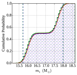
The bimodal distribution was composed of two copies of the unimodal multivariate Gaussian used above, with two mean vectors $\hat{\theta}_{i}$ and $\hat{\lambda}_{i}$ separated by $8\sigma$, as defined by $C_{ij}$. Using a bounding box at $\pm 9\sigma$ about the mid-point of the two modes, the evidence is calculated as $Z_{BM}^{\prime}\approx e^{-30.02}$.

The Rosenbrock “banana” function is a commonly used test function for optimisation algorithms Rosenbrock (1960). For this distribution, we do not have analytic one-dimensional marginal distributions to compare to, or known evidence values, so we were only able to do cross-comparisons between the samplers.

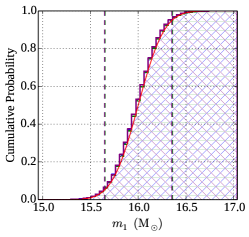
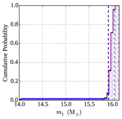
Each sampler was run targeting these known distributions, and the recovered posterior distributions and evidences were compared. The posterior distributions agreed for all parameter as expected, and an example of one parameter is shown in figure 6.

The recovered evidence values are shown in table 1. For the MCMC sampler the quoted errors come from the thermodynamic integration quadrature error estimates described in § IV.3; for the nested samplers the quoted errors are estimated by running the algorithm multiple times and computing the standard deviation of the results. For the simplest unimodal and bimodal distributions we see excellent agreement between the sampling methods, which agree within the $1\sigma$ statistical error estimates. The more difficult Rosenbrock likelihood results in a statistically significant disagreement between the nested sampling and BAMBI algorithms, with BAMBI returning the higher evidence estimate. To highlight the difficulty, for this problem the thermodynamic integration methods used with MCMC required 64 temperature ladder steps to reach convergence to $\beta\langle\log L\rangle=0$ at high temperatures, as opposed to the 16 used in the other problems. This pattern is repeated in the evidence for the signals, where there is a difference of several standard deviations between the methods.

V.2 Simulated GW signals

As an end-to-end test, we ran all three sampling flavours of LALInference (MCMC, section III.1; Nest, section III.2.1 and BAMBI, section III.2.2) on three test signals, described in table 2. These signals were injected into coloured Gaussian noise of known power spectrum and recovered with the same approximant used in generating the injection, listed in table 2. Since we used inspiral-only waveforms models for both injection and recovery, there is a sharp cutoff in the signal above the waveform’s termination frequency. It has been shown that in some circumstances the presence of this cutoff provides an artificially sharp feature which can improve parameter estimation beyond that of a realistic signal Mandel et al. (2014). Nonetheless, since the focus of this study is the consistency of the algorithms, we can proceed to use the sharply terminating waveforms for comparison purposes.

Fig.	Name	Approximant	$m_{1}$	$m_{2}$	$a_{1}$	$a_{2}$	$t_{1}$	$t_{2}$	$\iota$	distance	Network SNR
			$(\mathrm{M}_{\odot})$	$(\mathrm{M}_{\odot})$			(Rad)	(Rad)	$(\mbox{Rad})$	(Mpc)
7	BNS	TaylorF2 3.5PN	1.3382	1.249	0	0	-	-	2.03	135	13
8	NSBH	SpinTaylorT4 3.5PN	15	1.35	0.63	0	0	-	1.02	397	14
9	BBH	SpinTaylorT4 3.5PN	15	8	0.79	0.8	3.1	1.44	2.307	500	15

Table 2: Details of the injected signals used in section V.2, showing the waveform approximant used with the masses ($m_{\{1,2\}}$), spin magnitudes and tilt angles ($a_{\{1,2\}},t_{\{1,2\}}$), and the distance and inclination ($\iota$).

Figures 7, 8 and 9 show two-dimensional 90% credible intervals obtained by all three samplers on various combinations of parameters. Figure 7 (see table 2) shows the typical posterior structure for a BNS system. We show only three two-dimensional slices through the nine-dimensional (non-spinning) parameter space, highlighting the most relevant parameters for an astrophysical analysis. Selected one-dimensional 90% credible intervals are shown in table 5. This is the least challenging of the three example signals, since we restrict the model to non-spinning signals only. The posterior PDFs show excellent agreement between the sampling methods. In the leftmost panel we show the recovered distribution of the masses, parametrised by the chirp mass and symmetric mass ratio. This shows the high accuracy to which the chirp mass can be recovered compared to the mass ratio, which leads to a high degree of correlation between the estimated component masses. The domain of the prior ends at a maximum of $\eta=0.25$, which corresponds to the equal mass configuration. In the central panel we show the estimated sky location, which is well determined here thanks to the use of a three-detector network. In the rightmost panel, the correlation between the distance and inclination angle is visible, as both of these parameter scale the effective amplitude of the waveform. The reflection about the $\theta_{JN}=\pi/2$ line shows the degeneracy which is sampled efficiently using the extrinsic parameter jump proposals III.3.

Similarly to Figure 7, Figure 8 (see table 2) shows the posterior for a NSBH system. This signal was recovered using a spin-aligned waveform model, and we show six two-dimensional slices of this eleven-dimensional parameter space. Selected one-dimensional 90% credible intervals are shown in table 5. The top-left panel shows the $\mathcal{M}-\eta$ distribution; in comparison to Figure 7 the mass ratio is poorly determined. This is caused by the correlation between the $\eta$ parameter and the aligned spin magnitudes, which gives the model greater freedom in fitting $\eta$, varying $a_{1}$ and $a_{2}$ to compensate. This correlation is visible in the bottom-right panel. The other panels on the bottom row illustrate other correlations between the intrinsic parameters. The top-right panel shows the correlation between distance and inclination, where in this case the spins help break the degeneracy about the $\theta_{JN}=\pi/2$ line.

Lastly, figure 9 (see table 2) shows the posterior for a BBH system, recovered taking into account precession effect from two independent spins. We show nine two-dimensional slices of this fifteen-dimensional parameter space. One-dimensional 90% credible intervals are shown in table 5. In addition to the features similar to figure 7 in the top row, correlations with spin magnitudes (middle row) and tilt angles (bottom row) are shown. Note that the injected spin on the first component is almost anti-aligned with the orbital angular momentum, such that the tilt angle $t_{1}=3.1$, an unlikely random choice. This angle has a low prior probability, and as a result the injected value lies in the tails of the posterior distribution. This has repercussions in the recovered distributions for the spin magnitude and mass ratio, since they are partially degenerate in their effect on the phase evolution of the waveform, which results in the true value also being located in the tails of these distributions.

In all three cases, the three independent sampling algorithms converge on the same posterior distributions, indicating that the algorithms can reliably determine the source parameters, even for the full 15-dimensional spinning case.

	$\mathcal{M}$ ($\mathrm{M}_{\odot}$)	$\eta$	$m_{1}$ ($\mathrm{M}_{\odot}$)	$m_{2}$ ($\mathrm{M}_{\odot}$)	$d$ (Mpc)	$\alpha$ (rad)	$\delta$ (rad)
Nest	$1.1253^{1.1255}_{1.1251}$	$0.2487^{0.25}_{0.2447}$	$1.4^{1.5}_{1.3}$	$1.2^{1.3}_{1.1}$	$197^{251}_{115}$	$3.19^{3.24}_{3.14}$	$-0.997^{-0.956}_{-1.02}$
MCMC	$1.1253^{1.1255}_{1.1251}$	$0.2487^{0.25}_{0.2447}$	$1.4^{1.5}_{1.3}$	$1.2^{1.3}_{1.1}$	$195^{250}_{113}$	$3.19^{3.24}_{3.14}$	$-0.998^{-0.958}_{-1.02}$
BAMBI	$1.1253^{1.1255}_{1.1251}$	$0.2487^{0.25}_{0.2449}$	$1.4^{1.5}_{1.3}$	$1.2^{1.3}_{1.1}$	$196^{251}_{114}$	$3.19^{3.24}_{3.14}$	$-0.998^{-0.958}_{-1.02}$
Injected	1.1253	0.2497	1/3382	1.249	134.8	3.17	-0.97

Table 3: BNS recovered parameters. Median values and $5\%-95\%$ credible interval for a selection of parameters for each of the sampling algorithms.

	$\mathcal{M}(\mathrm{M}_{\odot})$	$\eta$	$m_{1}$ ($\mathrm{M}_{\odot}$)	$m_{2}$ ($\mathrm{M}_{\odot}$)	$d$ (Mpc)	$a_{1}$	$a_{2}$	$\alpha$ (rad)	$\delta$ (rad)
Nest	$3.42^{3.48}_{3.36}$	$0.11^{0.23}_{0.076}$	$11^{15}_{5.3}$	$1.7^{2.9}_{1.4}$	$612^{767}_{383}$	$0.36^{0.75}_{0.041}$	$0.49^{0.95}_{0.046}$	$0.843^{0.874}_{0.811}$	$0.459^{0.495}_{0.422}$
MCMC	$3.42^{3.48}_{3.36}$	$0.12^{0.23}_{0.077}$	$11^{15}_{5.3}$	$1.7^{2.9}_{1.4}$	$601^{763}_{369}$	$0.35^{0.73}_{0.038}$	$0.48^{0.94}_{0.045}$	$0.843^{0.874}_{0.812}$	$0.459^{0.496}_{0.422}$
BAMBI	$3.42^{3.48}_{3.37}$	$0.11^{0.22}_{0.075}$	$11^{15}_{5.8}$	$1.6^{2.7}_{1.3}$	$609^{767}_{378}$	$0.36^{0.72}_{0.042}$	$0.49^{0.95}_{0.044}$	$0.843^{0.874}_{0.811}$	$0.459^{0.495}_{0.422}$
Injected	3.477	0.076	15	1.35	397	0.63	0.0	0.82	0.44

Table 4: NSBH recovered parameters, defined as above.

	$\mathcal{M}$ ($\mathrm{M}_{\odot}$)	$\eta$	$m_{1}$ ($\mathrm{M}_{\odot}$)	$m_{2}$ ($\mathrm{M}_{\odot}$)	$d$ (Mpc)	$a_{1}$	$a_{2}$	$\alpha$ (rad)	$\delta$ (rad)
Nest	$9.5^{9.8}_{9.3}$	$0.15^{0.217}_{0.12}$	$24.3^{29.3}_{16.3}$	$5.5^{7.7}_{4.7}$	$647^{866}_{424}$	$0.34^{0.66}_{0.082}$	$0.48^{0.95}_{0.049}$	$0.21^{0.29}_{0.14}$	$-0.612^{-0.564}_{-0.659}$
MCMC	$9.5^{9.8}_{9.3}$	$0.15^{0.23}_{0.12}$	$23.8^{29.1}_{14.8}$	$5.5^{8.2}_{4.7}$	$630^{847}_{404}$	$0.36^{0.78}_{0.092}$	$0.51^{0.95}_{0.05}$	$0.21^{0.3}_{0.14}$	$-0.612^{-0.563}_{-0.658}$
BAMBI	$9.5^{9.8}_{9.3}$	$0.149^{0.216}_{0.12}$	$24.5^{29.2}_{16.3}$	$5.4^{7.5}_{4.7}$	$638^{859}_{428}$	$0.35^{0.69}_{0.087}$	$0.49^{0.94}_{0.049}$	$0.21^{0.29}_{0.14}$	$-0.612^{-0.565}_{-0.659}$
Injected	9.44	0.227	15	8	500	0.79	0.77	0.230	-0.617

Table 5: BBH recovered parameters, defined as above.

Figure 7: Comparison of probability density functions for the BNS signal (table 2) as determined by each sampler. Shown are selected 2D posterior density functions in greyscale, with red cross-hairs indicating the true parameter values, and contours indicating the 90% credible region as estimated by each sampler. On the axes are superimposed the one-dimensional marginal distributions for each parameter, as estimated by each sampler, and the true value indicated by a vertical red line. The colours correspond to blue: Bambi, magenta: Nest, green: MCMC. (left) The mass posterior distribution parametrized by chirp mass and symmetric mass ratio. (centre) The location of the source on the sky. (right) The distance $d_{L}$ and inclination $\theta_{JN}$ of the source showing the characteristic V-shaped degeneracy.

Figure 8: Comparison of probability density functions for the NSBH signal (table 2), with same color scheme as fig 7. (first row left) The mass posterior distribution parametrized by chirp mass and symmetric mass ratio. (first row centre) The location of the source on the sky. (first row right) The distance $d_{L}$ and inclination $\theta_{JN}$ of the source. In this case the V-shaped degeneracy is broken, but the large correlation between $d_{L}$ and $\theta_{JN}$ remains. (second row left) The spin magnitudes posterior distribution. (second row centre) The spin and mass of the most massive member of the binary illustrating the degeneracy between mass and spin. (second row right) The spin and symmetric mass ratio.

Figure 9: Comparison of probability density functions for the BBH signal (table 2), with same color scheme as fig 7. (first row left) The mass posterior distribution parametrized by chirp mass and symmetric mass ratio. (first row centre) The location of the source on the sky. (first row right) The distance $d_{L}$ and inclination $\theta_{JN}$ of the source showing the degeneracy is broken, as in the NSBH case. (second row left) The spins magnitude posterior distribution. (second row centre) The spin and mass of the most massive member of the binary illustrating the degeneracy between mass and spin. (second row right) The spin and symmetric mass ratio. (third row left) The spins tilt posterior distribution. (third row centre) The spin tilt of the more massive member of the binary and the symmetric mass ratio. (third row right) The spin tilt and mass of the most massive member of the binary.

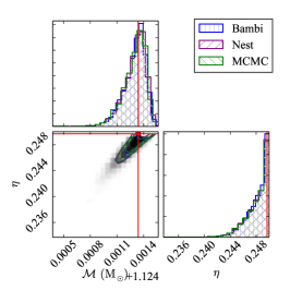
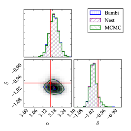
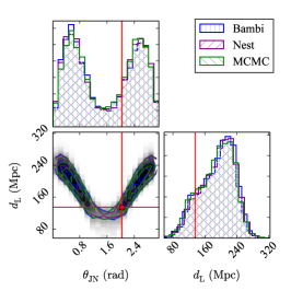
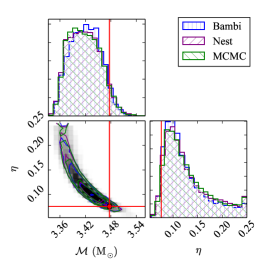
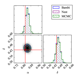
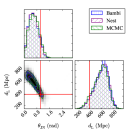
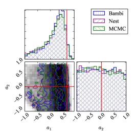
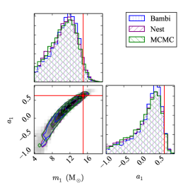
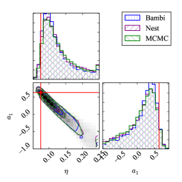
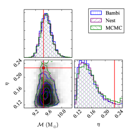
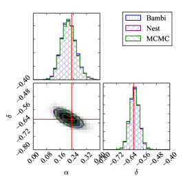
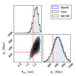
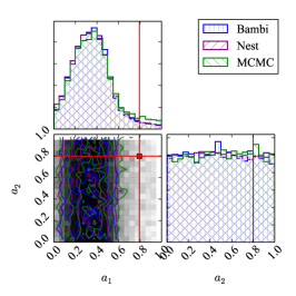
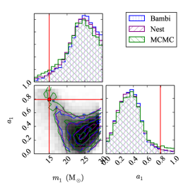
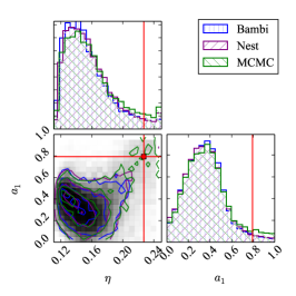
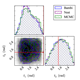
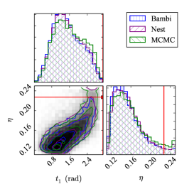
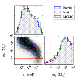
We also computed the evidence for each signal, relative to the Gaussian noise hypothesis, using each sampler, with errors computed as in § V.1. The results in table 1 show that the two flavours of nested sampling produce more precise estimates, according to their own statistical error estimates, but they disagree in the mean value. The thermodynamic integration method used with the MCMC algorithm (with 16 steps on the temperature ladder), produces a larger statistical error estimate, which generally encloses both the nested sampling and BAMBI estimates. These results indicate that there remains some systematic disagreement between the different methods of estimating evidence values, despite the good agreement between the posteriors. The BAMBI method generally produces a higher evidence estimate compared to the nested sampling approach, by around a factor of $e$. This indicates that further improvement is necessary before we can rely on these methods to distinguish models which are separated by evidence values lower than this factor.

V.3 Confidence intervals

Having checked the agreement of the posterior distributions on three selected injections, we performed a further check to ensure that the probability distributions we recover are truly representative of the confidence we should hold in the parameters of the signal. In the ideal case that our noise and waveform model matches the signal and noise in the data, and our prior distribution matches the set of signals in the simulations, then the recovered credible regions should match the probability of finding the true signal parameters within that region. By setting up a large set of test signals in simulated noise we can see if this is statistically true by determining the frequency with which the true parameters lie within a certain confidence level. This allows us to check that our credible intervals are well calibrated, in the sense of Dawid (1982).

For each run we calculate credible intervals from the posterior samples, for each parameter. We can then examine the number of times the injected value falls within a given credible interval. If the posterior samples are an unbiased estimate of the true probability, then $10\%$ of the runs should find the injected values within a $10\%$ credible interval, $50\%$ of runs within the $50\%$ interval, and so on.

We perform a KS-test on whether the results match the expected 1 to 1 relation between the fraction of signals in each credible region, and the level associated with that region.

For 1 dimensional tests our credible regions are defined as the connected region from the lowest parameter value to the value where the integrated probability reaches the required value. In practice we order the samples by parameter value and query what fraction of this list we count before passing the signal value.

To perform this test, we drew 100 samples from the prior distribution of section II.3, providing a set of injections to use for the test. This was performed using the TaylorF2 waveform approximant for both injection and recovery, with simulated Gaussian data using the initial LIGO and Virgo noise curves and 3 detector sites.

We calculated the cumulative distribution of the number of times the true value for each parameter was found within a given credible interval $p$, as a function of $p$, and compared the result to a perfect $1-1$ distribution using a KS test. All three codes passed this test for all parameters, indicating that our sampling and post-processing does indeed produce well-calibrated credible intervals. Figure 10 shows an example of the cumulative distribution of p-values produced by this test for the distance parameter. Similar plots were obtained for the other parameters.

Figure 10: P vs P plot for the distance parameter. On the $x$ axis is the probability $p$ contained in a credible interval, and on the $y$ axis the fraction of true values which lay inside that interval. The diagonal line indicates the ideal distribution where credible intervals perfectly reflect the frequency of recovered injections. For all three sampling algorithms the results are statistically consistent with the diagonal line, with the lowest KS statistic being $0.25$.

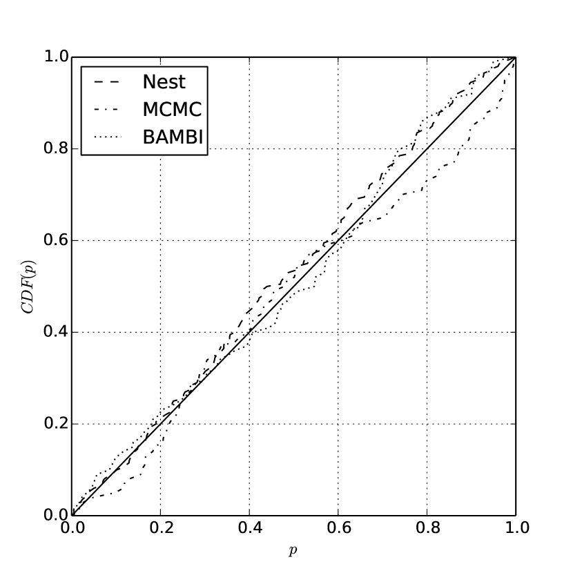
VI Computational Performance

We have benchmarked the three samplers using the three GW events described in section V.2. Although the specific performances listed are representative only of these signals, they do provide a rough idea of the relative computational performance of the sampling methods and the relative difficulty in the BNS, NSBH and BBH analyses, when running in a typical configuration. The computational cost of a parameter estimation run is strongly dependent on two main factors: the waveform family used (see sec. II.2) and the structure of the parameter space. Profiling of the codes show that computation of waveforms is the dominating factor, as the calculation of the phase evolution at each frequency bin is relatively expensive compared to the computation of the likelihood once the template is known.

The computationally easiest waveform to generate is TaylorF2, where an analytic expression for the waveform in the frequency domain is available. For the BNS signal simulated here, around 50 waveforms can be generated per second at our chosen configuration ($32\,$s of data sampled at $4096\,$Hz). On the other hand, more sophisticated waveforms, like SpinTaylorT4 with precessing spins, require solving differential equations in the time domain, and a subsequent FFT (the likelihood is always calculated in the frequency domain), which raises the CPU time required to generate a single waveform by an order of magnitude.

The structure of the parameter space affects the length of a run in several ways. The first, and most obvious, is through the number of dimensions: when waveforms with precessing spins are considered a 15-dimension parameter space must be explored, while in the simpler case of non-spinning signals the number of dimensions is 9. The duration of a run will also depend on the correlations present in the parameter space, e.g. between the distance and inclination parameters Aasi et al. (2013). Generally speaking runs where correlations are stronger will take longer to complete as the codes will need more template calculations to effectively sample the parameter space and find the region of maximum likelihood.

Table 6 shows a comparison of the efficiency of each code running on each of the simulated signals in terms of the cost in CPU time, wall time, and the CPU/wall time taken to generate each sample which ended up in the posterior distribution. These numbers were computed using the same hardware, Intel Xeon E5-2670 2.6 GHz processors.

We note that at the time of writing the three samplers have different level of parallelization, which explains the differences between codes of the ratio CPU time to wall time.

BNS	Bambi	Nest	MCMC
posterior samples	6890	19879	8363
CPU time (s.)	3317486	1532692	725367
wall time (s.)	219549	338175	23927
CPU seconds/sample	481.5	77.1	86.7
wall seconds/sample	31.9	17.0	2.9
NSBH	Bambi	Nest	MCMC
posterior samples	7847	20344	10049
CPU time (s.)	2823097	9463805	4854653
wall time (s.)	178432	2018936	171992
CPU seconds/sample	359.8	465.2	483.1
wall seconds/sample	22.7	99.2	17.1
BBH	Bambi	Nest	MCMC
posterior samples	10920	34397	10115
CPU time (s.)	2518763	7216335	5436715
wall time (s.)	158681	1740435	200452
CPU seconds/sample	230.7	209.8	537.5
wall seconds/sample	14.5	50.6	19.8

Table 6: Preformance of all three sampling methods on the three signals from table 2. The time quoted in the “CPU time” line is the cumulative CPU-time across multiple cores, while the time quoted in the “wall time” line is the actual time taken to complete the sampling. The difference is an indication of the varying degrees of parallelism in the methods.

VII Conclusions and future goals

In this paper we have described the application of three stochastic sampling algorithms to the problem of compact binary parameter estimation and model selection. Their implementation in the LALInference package provides a flexible and open-source toolkit which builds upon much previous work to give reliable results  Rodriguez et al. (2014); van der Sluys et al. (2008a); Vitale et al. (2014); Christensen and Meyer (2001); Christensen et al. (2004); Röver et al. (2006, 2007); van der Sluys et al. (2008a, b); Raymond et al. (2009); van der Sluys et al. (2009); Raymond et al. (2010); Veitch and Vecchio (2010); Feroz et al. (2009, 2013); Graff et al. (2012). The independent sampling methods have allowed us to perform detailed cross-validation of the results of inference on a range of GW signals from compact binary coalescences, such as will be observed by future gravitational-wave detectors. We have also performed internal consistency checks of the recovered posterior distributions to ensure that the quoted credible intervals truly represent unbiased estimates of the parameters under valid prior assumptions.

The release of the LALInference toolkit as part of the open-source LAL package, available from LAL , has already provided a base for developing methods for testing general relativity Del Pozzo et al. (2011); Li et al. (2012); Agathos et al. (2014) and performing parameter estimation on a variety of other GW sourcesPitkin et al. (2012); Logue et al. (2012). In the future we intend to further develop the implementation to accommodate more sophisticated noise models for data analysis in the advanced detector era. This will enable us to provide parameter estimation results which are robust against the presence of glitches in the data, against time-dependent fluctuations in the noise spectrumRöver et al. (2011); Littenberg et al. (2013); Littenberg and Cornish (2014), and will allow us to incorporate uncertainty in the calibration of the instruments.

Work is also ongoing in improving inference to incorporate systematic uncertainties in the waveform models which affect estimates of intrinsic parameters Aasi et al. (2013).

Meanwhile, recent advances in reduced order modelling of the waveforms and developments of surrogate models for the most expensive waveforms should result in a dramatic improvement in the speed of parameter estimation Field et al. (2014); Canizares et al. (2013); Purrer:2014fza; Canizares et al. (2014). More intelligent proposal distributions also have the potential to reduce the autocorrelation timescales in the MCMC and Nested Sampling algorithms, further improving the efficiency of these methods.

The work described here should serve as a foundation for these further developments, which will be necessary to fully exploit the science capabilities of the advanced generation of gravitational-wave detectors, and produce parameter estimates in a timely manner.

References

- Abbott et al. (2009) B. Abbott et al. (LIGO Scientific Collaboration), Rept. Prog. Phys. 72, 076901 (2009), eprint 0711.3041.
- Acernese et al. (2008) F. Acernese et al., Class. Quantum Grav. 25, 114045 (2008).
- Grote (2010) H. Grote (LIGO Scientific Collaboration), Class.Quant.Grav. 27, 084003 (2010).
- Harry and the LIGO Scientific Collaboration (2010) G. M. Harry and the LIGO Scientific Collaboration, Class. Quantum Gravity 27, 084006 (2010), eprint arXiv:1103.2728.
- Virgo Collaboration (2009) Virgo Collaboration, Virgo Technical Report VIR-0027A-09 (2009), URL https://tds.ego-gw.it/itf/tds/file.php?callFile=VIR-0027A-09.pdf.
- Kuroda (2011) K. Kuroda (LCGT Collaboration), Int.J.Mod.Phys. D20, 1755 (2011).
- Unnikrishnan (2013) C. S. Unnikrishnan, International Journal of Modern Physics D 22, 1341010 (2013).
- gw_(2013) Tech. Rep. LIGO-P1200087, The LIGO Scientific Collaboration and the Virgo Collaboration (2013), URL https://dcc.ligo.org/LIGO-P1200087/public.
- Abadie et al. (2010) J. Abadie et al. (LIGO Scientific Collaboration and Virgo Collaboration), Class. Quantum Grav. 27, 173001 (2010).
- Babak et al. (2013) S. Babak, R. Biswas, P. R. Brady, D. A. Brown, K. Cannon, C. D. Capano, J. H. Clayton, T. Cokelaer, J. D. E. Creighton, T. Dent, et al., Phys. Rev. D 87, 024033 (2013), eprint 1208.3491.
- Cannon et al. (2012) K. Cannon et al., The Astrophysical Journal 748, 136 (2012), URL http://stacks.iop.org/0004-637X/748/i=2/a=136.
- Abadie et al. (2012) J. Abadie et al. (LIGO Collaboration, Virgo Collaboration), Phys.Rev. D85, 082002 (2012), eprint 1111.7314.
- Christensen and Meyer (2001) N. Christensen and R. Meyer, Phys.Rev. D64, 022001 (2001), eprint gr-qc/0102018.
- Christensen et al. (2004) N. Christensen, R. Meyer, and A. Libson, Class. Quantum Grav. 21, 317 (2004).
- Röver et al. (2006) C. Röver, R. Meyer, and N. Christensen, Classical and Quantum Gravity 23, 4895 (2006), eprint gr-qc/0602067.
- Röver et al. (2007) C. Röver, R. Meyer, and N. Christensen, Phys. Rev. D 75, 062004 (2007), eprint gr-qc/0609131.
- van der Sluys et al. (2008a) M. V. van der Sluys, C. Röver, A. Stroeer, V. Raymond, I. Mandel, N. Christensen, V. Kalogera, R. Meyer, and A. Vecchio, ApJ 688, L61 (2008a), eprint 0710.1897.
- van der Sluys et al. (2008b) M. van der Sluys, V. Raymond, I. Mandel, C. Röver, N. Christensen, V. Kalogera, R. Meyer, and A. Vecchio, Classical and Quantum Gravity 25, 184011 (2008b), eprint 0805.1689.
- Raymond et al. (2009) V. Raymond, M. V. van der Sluys, I. Mandel, V. Kalogera, C. Röver, and N. Christensen, Classical and Quantum Gravity 26, 114007 (2009), eprint 0812.4302.
- van der Sluys et al. (2009) M. van der Sluys, I. Mandel, V. Raymond, V. Kalogera, C. Röver, and N. Christensen, Classical and Quantum Gravity 26, 204010 (2009), eprint 0905.1323.
- Raymond et al. (2010) V. Raymond, M. V. van der Sluys, I. Mandel, V. Kalogera, C. Röver, and N. Christensen, Classical and Quantum Gravity 27, 114009 (2010), eprint 0912.3746.
- Skilling (2006) J. Skilling, Bayesian Analysis 1, 833 (2006).
- Veitch and Vecchio (2010) J. Veitch and A. Vecchio, Phys. Rev. D 81, 062003 (2010), eprint 0911.3820.
- Feroz and Hobson (2008) F. Feroz and M. P. Hobson, MNRAS 384, 449 (2008), eprint 0704.3704.
- Feroz et al. (2009) F. Feroz, M. P. Hobson, and M. Bridges, MNRAS 398, 1601 (2009), eprint 0809.3437.
- Feroz et al. (2013) F. Feroz, M. P. Hobson, E. Cameron, and A. N. Pettitt, ArXiv e-prints (2013), eprint 1306.2144.
- Graff et al. (2012) P. Graff, F. Feroz, M. P. Hobson, and A. Lasenby, MNRAS 421, 169 (2012), eprint 1110.2997.
- Veitch et al. (2012) J. Veitch, I. Mandel, B. Aylott, B. Farr, V. Raymond, C. Rodriguez, M. van der Sluys, V. Kalogera, and A. Vecchio, Phys. Rev. D 85, 104045 (2012), eprint 1201.1195.
- Rodriguez et al. (2014) C. L. Rodriguez, B. Farr, V. Raymond, W. M. Farr, T. B. Littenberg, et al., Astrophys.J. 784, 119 (2014), eprint 1309.3273.
- Vitale et al. (2014) S. Vitale, R. Lynch, J. Veitch, V. Raymond, and R. Sturani, Phys. Rev. Lett. 112, 251101 (2014), URL http://link.aps.org/doi/10.1103/PhysRevLett.112.251101.
- Blackburn et al. (2013) L. Blackburn, M. S. Briggs, J. Camp, N. Christensen, V. Connaughton, et al. (2013), eprint 1303.2174.
- Grover et al. (2014) K. Grover, S. Fairhurst, B. F. Farr, I. Mandel, C. Rodriguez, et al., Phys.Rev. D89, 042004 (2014), eprint 1310.7454.
- Del Pozzo et al. (2013a) W. Del Pozzo, T. G. F. Li, M. Agathos, C. Van Den Broeck, and S. Vitale, Phys. Rev. Lett. 111, 071101 (2013a), eprint 1307.8338.
- Vitale et al. (2012) S. Vitale, W. Del Pozzo, T. G. F. Li, C. Van Den Broeck, I. Mandel, B. Aylott, and J. Veitch, Phys. Rev. D 85, 064034 (2012), eprint 1111.3044.
- Del Pozzo et al. (2011) W. Del Pozzo, J. Veitch, and A. Vecchio, Phys. Rev. D 83, 082002 (2011), eprint 1101.1391.
- Li et al. (2012) T. G. F. Li, W. Del Pozzo, S. Vitale, C. Van Den Broeck, M. Agathos, J. Veitch, K. Grover, T. Sidery, R. Sturani, and A. Vecchio, Phys. Rev. D 85, 082003 (2012), eprint 1110.0530.
- Agathos et al. (2014) M. Agathos, W. Del Pozzo, T. G. F. Li, C. V. D. Broeck, J. Veitch, et al., Phys.Rev. D89, 082001 (2014), eprint 1311.0420.
- Aasi et al. (2013) J. Aasi, J. Abadie, B. P. Abbott, R. Abbott, T. D. Abbott, M. Abernathy, T. Accadia, F. Acernese, C. Adams, T. Adams, et al., Phys. Rev. D 88, 062001 (2013), eprint 1304.1775.
- Aasi et al. (2014) J. Aasi et al. (LIGO Scientific Collaboration, Virgo Collaboration, NINJA-2 Collaboration), Class.Quant.Grav. 31, 115004 (2014), eprint 1401.0939.
- Pitkin et al. (2012) M. Pitkin, C. Gill, J. Veitch, E. Macdonald, and G. Woan, J.Phys.Conf.Ser. 363, 012041 (2012), eprint 1203.2856.
- Logue et al. (2012) J. Logue, C. D. Ott, I. S. Heng, P. Kalmus, and J. H. C. Scargill, Phys.Rev. D86, 044023 (2012), eprint 1202.3256.
- Röver et al. (2011) C. Röver, R. Meyer, and N. Christensen, Classical and Quantum Gravity 28, 015010 (2011).
- Littenberg et al. (2013) T. B. Littenberg, M. Coughlin, B. Farr, and W. M. Farr, Phys. Rev. D 88, 084044 (2013), eprint 1307.8195.
- Cornish and Littenberg (2014) N. J. Cornish and T. B. Littenberg (2014), eprint 1410.3835.
- Littenberg and Cornish (2014) T. B. Littenberg and N. J. Cornish (2014), eprint 1410.3852.
- Anderson et al. (2001) W. G. Anderson, P. R. Brady, J. D. E. Creighton, and E. E. Flanagan, Phys. Rev. D 63, 042003 (2001), eprint gr-qc/0008066.
- (47) LSC Algorithm Library software packages lal, lalwrapper, and lalapps, URL http://www.lsc-group.phys.uwm.edu/lal.
- Allen et al. (2012) B. Allen, W. G. Anderson, P. R. Brady, D. A. Brown, and J. D. E. Creighton, Phys.Rev. D85, 122006 (2012), eprint gr-qc/0509116.
- Finn (1996) L. S. Finn, Phys. Rev. D 53, 2878 (1996), eprint arXiv:gr-qc/9601048.
- Röver (2011) C. Röver, Phys. Rev. D 84, 122004 (2011), URL http://link.aps.org/doi/10.1103/PhysRevD.84.122004.
- Farr et al. (2014) B. Farr, E. Ochsner, W. M. Farr, and R. O’Shaughnessy, Phys.Rev. D90, 024018 (2014), eprint 1404.7070.
- Del Pozzo et al. (2013b) W. Del Pozzo, T. G. F. Li, M. Agathos, C. Van Den Broeck, and S. Vitale, Physical Review Letters 111, 071101 (2013b), eprint 1307.8338.
- Yunes and Pretorius (2009) N. Yunes and F. Pretorius, Phys. Rev. D 80, 122003 (2009), eprint 0909.3328.
- Konigsdorffer and Gopakumar (2006) C. Konigsdorffer and A. Gopakumar, Phys.Rev. D73, 124012 (2006), eprint gr-qc/0603056.
- Aasi et al. (2013) J. Aasi et al. (LIGO Collaboration, Virgo Collaboration), Phys.Rev. D88, 062001 (2013), eprint 1304.1775.
- Buonanno et al. (2009) A. Buonanno, B. R. Iyer, E. Ochsner, Y. Pan, and B. S. Sathyaprakash, Phys.Rev. D80, 084043 (2009), eprint 0907.0700.
- Buonanno et al. (2003) A. Buonanno, Y. Chen, and M. Vallisneri, Phys. Rev. D 67, 104025 (2003), erratum-ibid. 74 (2006) 029904(E).
- Ajith et al. (2011) P. Ajith, M. Hannam, S. Husa, Y. Chen, B. Brügmann, N. Dorband, D. Müller, F. Ohme, D. Pollney, C. Reisswig, et al., Phys. Rev. Lett. 106, 241101 (2011), eprint 0909.2867.
- Pan et al. (2011) Y. Pan, A. Buonanno, M. Boyle, L. T. Buchman, L. E. Kidder, H. P. Pfeiffer, and M. A. Scheel, Phys. Rev. D 84, 124052 (2011), eprint 1106.1021.
- Brown (2004) D. A. Brown (2004), eprint arXiv:0705.1514v1 [gr-qc].
- Metropolis et al. (1953) N. Metropolis, A. W. Rosenbluth, M. N. Rosenbluth, A. H. Teller, and E. Teller, J. Chem. Phys. 21, 1087 (1953).
- Hastings (1970) W. K. Hastings, Biometrika 57, 97 (1970), URL http://biomet.oxfordjournals.org/content/57/1/97.abstract.
- Gelman et al. (1996) A. Gelman, G. Roberts, and W. Gilks, Bayesian statistics 5, 599 (1996).
- Roberts and Rosenthal (1998) G. O. Roberts and J. S. Rosenthal, Canadian Journal of Statistics 26, 5 (1998), ISSN 1708-945X, URL http://dx.doi.org/10.2307/3315667.
- Gilks et al. (1996) W. R. Gilks, S. Richardson, and D. J. Spiegelhalter, Markov chain Monte Carlo in practice (Chapman and Hall / CRC, 1996).
- Earl and Deem (2005) D. J. Earl and M. W. Deem, Phys. Chem. Chem. Phys. 7, 3910 (2005).
- Forum (1994) M. P. Forum, Tech. Rep., Knoxville, TN, USA (1994).
- Graff et al. (2014) P. Graff, F. Feroz, M. P. Hobson, and A. Lasenby, MNRAS 441, 1741 (2014), eprint 1309.0790.
- ter Braak (2006) C. ter Braak, Statistics and Computing 16, 239 (2006), ISSN 0960-3174, URL http://dx.doi.org/10.1007/s11222-006-8769-1.
- ter Braak and Vrugt (2008) C. ter Braak and J. Vrugt, Statistics and Computing 18, 435 (2008), ISSN 0960-3174, URL http://dx.doi.org/10.1007/s11222-008-9104-9.
- Roberts and Rosenthal (2001) G. O. Roberts and J. S. Rosenthal, Statistical Science 16, pp. 351 (2001), ISSN 08834237, URL http://www.jstor.org/stable/3182776.
- Roberts and Rosenthal (2007) G. O. Roberts and J. S. Rosenthal, J. App. Prob. 44, 458 (2007).
- Raymond and Farr (2014) V. Raymond and W. Farr (2014), eprint 1402.0053.
- Raftery et al. (2007) A. E. Raftery, M. A. Newton, J. M. Satagopan, and P. N. Krivitsky, in Bayesian Statistics (2007), pp. 1–45.
- Newton and Raftery (1994) M. A. Newton and A. E. Raftery, J. R. Stat. Soc. B 56, 3 (1994).
- Chib (1995) S. Chib, J. Am. Stat. Assoc. 90, 1313 (1995).
- van Haasteren (2009) R. van Haasteren, ArXiv e-prints (2009), arXiv:0911.2150.
- Weinberg (2009) M. D. Weinberg, ArXiv e-prints (2009), eprint 0911.1777.
- R. M. Neal (1993) R. M. Neal, Tech. Rep. CRG-TR-93-1, Department of Computer Science, University of Toronto (1993), http://omega.albany.edu:8008/neal.pdf.
- Littenberg and Cornish (2009) T. B. Littenberg and N. J. Cornish, Phys. Rev. D 80, 063007 (2009), eprint 0902.0368.
- Sidery et al. (2014) T. Sidery, W. Farr, J. Gair, and I. Mandel, Tech. Rep. P1400054, LIGO-Virgo Collaboration (2014), URL https://dcc.ligo.org/LIGO-P1400054/public.
- Rosenbrock (1960) H. H. Rosenbrock, The Computer Journal 3, 175 (1960).
- Mandel et al. (2014) I. Mandel, C. P. Berry, F. Ohme, S. Fairhurst, and W. M. Farr, Class.Quant.Grav. 31, 155005 (2014), eprint 1404.2382.
- Dawid (1982) A. P. Dawid, Journal of the American Statistical Association 77, 605 (1982).
- Field et al. (2014) S. E. Field, C. R. Galley, J. S. Hesthaven, J. Kaye, and M. Tiglio, Phys.Rev. X4, 031006 (2014), eprint 1308.3565.
- Canizares et al. (2013) P. Canizares, S. E. Field, J. R. Gair, and M. Tiglio, Phys.Rev. D87, 124005 (2013), eprint 1304.0462.
- Canizares et al. (2014) P. Canizares, S. E. Field, J. Gair, V. Raymond, R. Smith, et al. (2014), eprint 1404.6284.
- (88) D. Foreman-Mackay et al., triangle.py, URL http://dx.doi.org/10.5281/zenodo.11020.