Parameter estimation for binary neutron-star coalescences with realistic noise during the Advanced LIGO era

Abstract

Advanced ground-based gravitational-wave (GW) detectors begin operation imminently. Their intended goal is not only to make the first direct detection of GWs, but also to make inferences about the source systems. Binary neutron-star mergers are among the most promising sources. We investigate the performance of the parameter-estimation ipeline that will be used during the first observing run of the Advanced Laser Interferometer Gravitational-wave Observatory (aLIGO) in 2015: we concentrate on the ability to reconstruct the source location on the sky, but also consider the ability to measure masses and the distance. Accurate, rapid sky-localization is necessary to alert electromagnetic (EM) observatories so that they can perform follow-up searches for counterpart transient events. We consider PE accuracy in the presence of non-Gaussian noise. We find that the character of the noise makes negligible difference to the PE performance The source luminosity distance can only be poorly constrained, the median $90\%$ ($50\%$) credible interval scaled with respect to the true distance is $0.85$ ($0.38$). However, the chirp mass is well measured. Our chirp-mass estimates are subject to systematic error because we used gravitational-waveform templates without component spin to carry out inference on signals with moderate spins, but the total error is typically less than $10^{-3}M_{\odot}$. The median $90\%$ ($50\%$) credible region for sky localization is $\sim 600~{}\mathrm{deg^{2}}$ ($\sim 150~{}\mathrm{deg^{2}}$), with $3\%$ ($30\%$) of detected events localized within $100~{}\mathrm{deg^{2}}$. Early aLIGO, with only two detectors, will have a sky-localization accuracy for binary neutron stars of hundreds of square degrees; this makes EM follow-up challenging, but not impossible.

1. Introduction

The goal of gravitational-wave (GW) astronomy is to learn about the Universe through observations of gravitational radiation. This requires not only the ability to detect GWs, but also to infer the properties of their source systems. In this work, we investigate the ability to perform parameter estimation (PE) on signals detected by the upcoming Advanced LIGO (aLIGO) instruments (Harry:2010zz; TheLIGOScientific:2014jea) in the initial phase of their operation (Aasi:2013wya).

Compact binary coalescences (CBCs), the GW-driven inspiral and merger of stellar-mass compact objects, are a prime source for aLIGO and Advanced Virgo (AdV; AdvVirgo; TheVirgo:2014hva). Binary neutron-star (BNS) systems may be the most abundant detectable CBCs (Abadie:2010cf). We focus on BNS mergers in this study.

Following the identification of a detection candidate, we wish to extract the maximum amount of information from the signal. It is possible to make some inferences using selected components of the data. However, full information regarding the source system, including the component objects’ masses and spins, is encoded within the gravitational waveform, and can be obtained by comparing the data to theoretical waveform models (Cutler:1994ys; Jaranowski:2007pe). Doing so can be computationally expensive.

PE is performed within a Bayesian framework. We use algorithms available as part of the LALInference toolkit for the analysis of CBC signals. The most expedient code is bayestar (Singer:2014qca; Singer:2014), which infers sky location from data returned from the detection pipeline. Exploring the posterior probability densities for the parameters takes longer for models where the parameter space is larger or the likelihood is more complicated. Calculating estimates for parameters beyond sky location is done using the stochastic-sampling algorithms of LALInference (Veitch:2014wba). There are three interchangeable sampling algorithms: LALInference_nest (Veitch:2009hd), LALInference_mcmc (vanderSluys:2008qx; Raymond:2008im) and LALInference_bambi (Graff:2011gv), which we refer to as LALInference for short. These compute waveform templates for use in the likelihood. Using the least computationally expensive waveforms allows for posteriors to be estimated on timescales of hours to days; potentially more accurate estimates can be calculated with more expensive waveforms. In this paper, we discuss what can be achieved using low-latency (bayestar) and medium-latency (LALInference with inexpensive waveforms) PE; a subsequent paper will evaluate what can be achieved on longer timescales using more expensive waveform templates.

With the detection of GWs, it is also possible to perform multi-messenger astronomy, connecting different types of observations of the same event. BNS mergers could be accompanied by an electromagnetic (EM) counterpart (Metzger:2011bv). To associate an EM event with a GW signal, it is beneficial to have an accurate sky location: timing information can also be used for EM signals that are independently detected, such as gamma-ray bursts (Aasi:2014iia). To provide triggers for telescopes to follow up a GW detection, it is necessary to provide rapid sky localization.

Several large-scale studies investigated the accuracy with which sky position can be reconstructed from observations with ground-based detector networks. The first only used timing information from a multi-detector network to triangulate the source position on the sky (e.g., Fairhurst:2009tc; Fairhurst:2010is). Subsequently, further information about the phase of the gravitational waveform was folded into the timing triangulation (TT) analysis (Grover:2013sha). The most sophisticated techniques perform a coherent Bayesian analysis to reconstruct probability distributions for the sky location (e.g., Veitch:2012df; Nissanke:2012dj; Kasliwal:2013yqa; Grover:2013sha; Sidery:2013zua). Singer:2014qca used both bayestar and LALInference to analyse the potential performance of aLIGO and AdV in the first two years of their operation. They assumed the detector noise was stationary and Gaussian. Here, we further their studies (although we use the same analysis pipeline) by using a set of injections into observed noise from initial LIGO detectors recoloured (see section 2.1) to the expected spectral density of early aLIGO. This provides results closer to those expected in practice, as real interferometer noise includes features such as non-stationary glitches (Aasi:2013wya; Aasi:2014usa). Our results are just for the first observing run (O1) of aLIGO, expected in the latter half of 2015, assuming that this occurs before the introduction of AdV. As the sensitivity of the detectors will increase with time, and because the introduction of further detectors increases the accuracy of sky localization (Schutz:2011tw), these set a lower bound for the advanced-detector era. Estimates for sky-localization accuracy in later observing periods can be calibrated using our results.

PE beyond sky localization, considering the source system’s mass, spin, distance and orientation, has been subject to similar studies. The initial investigations estimated PE using the Fisher information matrix (e.g., Cutler:1994ys; Poisson:1995ef; Arun:2004hn). nly gives an approximation to true PE potential (Vallisneri:2007ev). More reliable (but computationally expensive) results are found by simulating a GW event and analysing it using PE codes, mapping the posterior probability distributions (e.g., Rover:2006ni; vanderSluys:2007st; Veitch:2009hd; Rodriguez:2013oaa). This has even been done for a blind injection during the run of initial LIGO (Aasi:2013jjl). As with sky-localization, general PE can improve with the introduction of more detectors to the network (Veitch:2012df).

To be as faithful as possible, our analysis is performed using one of the pipelines intended for use during O1. We make use of IGO Scientific Collaboration Algorithm Library (LAL). In particular, we shall make use of GSTLAL, one of the detection pipelines, to search for signals and LALInference for PE on detection candidates.

We begin by describing the source catalogue and detector sensitivity curve used for this study in section 2. In section 3 we explain how the data is analysed to produce sky areas and other parameter estimates. In section 4 we present the results of our work. We first discuss the set of events that are selected by the detection pipeline in section 4.1 (with supplementary information in appendix LABEL:ap:mass); then we examine PE, considering sky-localization accuracy in section 4.2, and mass and distance measurements in section 4.3. We conclude with a discussion of these results in section LABEL:sec:end; this includes in section LABEL:sec:three-det an analysis of estimates for sky localization in later observing periods with reference to our findings. Estimates of the computational costs associated with running bayestar and full LALInference PE are given in appendix LABEL:ap:cost. Our main findings are:

1. The detection pipeline returns a population of sources that is not significantly different from the input astrophysical population, despite a selection bias based upon the chirp mass.

2. Both bayestar and LALInference return comparable sky-localization accuracies (for a two-detector network). The latter takes more computational time (a total CPU time of $\sim 10^{6}~{}\mathrm{s}$ per event compared with $\sim 10^{3}~{}\mathrm{s}$), but returns estimates for more parameters than just location.

3. At a given signal-to-noise ratio (SNR), the character of the noise does not affect sky localization or other PE.

4. Switching from a detection threshold based upon SNR to one based upon the false alarm rate (FAR) changes the SNR-distribution of detected events. A selection based upon FAR includes more low-SNR events (the distribution at high SNRs is unaffected).

5. TT provides a poor predictor of sky localization for a two-detector network; it does better (on average) for a three-detector network when phase coherence is included, but remains imperfect.

6. Systematic errors from uncertainty in the waveform template are significant for chirp-mass estimation. Neglecting the mass–spin degeneracy by using non-spinning waveforms artificially narrows the posterior distribution.

For O1, we find that the luminosity distance is not well-measured, the median $50\%$ credible interval (interquartile range) divided by the true distance is $0.38$ and the median $90\%$ credible interval divided by the true distance is $0.85$. Despite being subject to systematic error, the chirp mass is still accurately measured, with the posterior mean being less than $10^{-3}M_{\odot}$ from the true value ll ($96\%$) cases. We find that the median area of $50\%$ sky localization credible region is $154~{}\mathrm{deg^{2}}$ and the median area of the $90\%$ credible region is $632~{}\mathrm{deg^{2}}$; the median searched area (area of the smallest credible region that encompasses the source location) is $132~{}\mathrm{deg^{2}}$. EM follow-up to BNS mergers in 2015 will be challenging and require careful planning.

2. Sources and sensitivities

Our input data consists of two components: simulated detector noise and simulated BNS signals. We describe the details of these in the following subsections, before continuing with the analysis of the data in section 3.

2.1. Recoloured 2015 noise

We consider the initial operation of the advanced detectors at LIGO Hanford and LIGO Livingston. The sensitivity is assumed to be given by the early curve of Barsotti:2012, which has a BNS detection range of $\sim 55~{}\mathrm{Mpc}$ (assuming Gaussian noise). This configuration corresponds to the 2015 observing scenario in Aasi:2013wya. Figure 1 plots the noise spectral density, the square root of the power spectral density (Moore:2014lga), as measured during the sixth science (S6) run of initial LIGO, the early aLIGO sensitivity curve, and final aLIGO curve (Shoemaker:2010).

Figure 1.— Initial and Advanced LIGO noise amplitude spectral densities. The upper line is the measured sensitivity of the initial LIGO Hanford detector during S6 (Aasi:2014usa). The dashed line shows the early aLIGO sensitivity and the lower solid line the final sensitivity (Barsotti:2012). The early sensitivity is used as a base here.

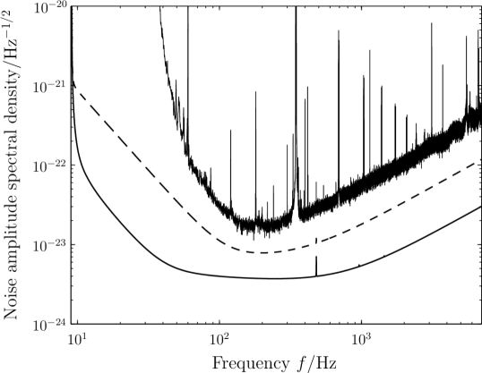
The noise is constructed from data from the S6 run of initial LIGO (Christensen:2010zz; Aasi:2014usa), recoloured to the early aLIGO noise spectral density as was done for Aasi:2014tra.

2.2. Binary neutron-star events

BNS systems constitute the most probable and best understood source of signals for advanced ground-based GW detectors. There is a wide range in predicted event rates as a consequence of uncertainty in our knowledge of the astrophysics. Abadie:2010cf gives a BNS merger rate for the full-sensitivity aLIGO–AdV network of $0.01$–$10~{}\mathrm{Mpc^{-3}\,Myr^{-1}}$, with $1~{}\mathrm{Mpc^{-3}\,Myr^{-1}}$ as the most realistic estimate (Kalogera:2003tn).

We use the same list of simulated sources as in Singer:2014qca. The neutron-star masses are uniformly distributed from $m_{\mathrm{min}}=1.2M_{\odot}$ to $m_{\mathrm{max}}=1.6M_{\odot}$, which safely encompasses the observed mass range of BNS systems (Kiziltan:2013oja). Their (dimensionless) spin magnitudes are uniformly distributed between $a_{\mathrm{min}}=0$ and $a_{\mathrm{max}}=0.05$. s PSR J0737$-$3039A (Burgay:2003jj; Kramer:2009zza). This has been estimated to have a spin within this range (Mandel:2009nx; Brown:2012qf): since we do not know precisely the neutron-star equation of state (Lattimer:2012nd), it is not possible to exactly convert from a spin period to a spin magnitude. The spin orientations are distributed isotropically. The binaries are uniformly scattered in volume and This set of parameters is motivated by our understanding of the astrophysical population of BNSs.

The GW signals were constructed using a post-Newtonian (PN) inspiral template, the SpinTaylorT4 approximant (Buonanno:2002fy; Buonanno:2009zt) which is a time-domain approximant accurate to 3.5PN order in phase and 1.5PN order in amplitude. There exist more accurate but more expensive waveforms. This template only contains the inspiral part of the waveform and not the subsequent merger: this should happen outside of the sensitive band of the detector for the masses considered and so should not influence PE (Mandel:2014tca). instead we use a less expensive approximant. In a future study, we shall investigate the effects of using SpinTaylorT4 templates for PE, such that the injection and recovery templates perfectly match.

3. Analysis pipeline

To accurately forecast sky localization prospects in O1, we run our simulated events through the same data-analysis pipeline as is intended for real data. The results of this pipeline are analysed in the next section (section 4). A GW search is performed using GSTLAL_inspiral (Cannon:2010qh; Cannon:2011tb; Cannon:2011vi; Cannon:2012zt); this is designed to provide GW triggers in real time with $\sim 10$–$100~{}\mathrm{s}$ latency during LIGO–Virgo observing runs. A trigger is followed up for sky localization if its calculated FAR is less than $10^{-2}~{}\mathrm{yr^{-1}}$, which is roughly equivalent to a network-SNR threshold of $\varrho\gtrsim 12$ (Aasi:2013wya).

In using the FAR to select triggers, our method differs from that used in Singer:2014qca. Since they considered Gaussian noise, which is free of glitches, their FAR would not be representative of those computed using real noise; the FAR calculated with Gaussian noise corresponds to a SNR-threshold that is too low for detection in realistic noise. Therefore, they also imposed a network-SNR cut of $\varrho\geq 12$, in addition to the FAR selection. This joint SNR and FAR threshold was found to differ negligibly from an SNR-only threshold: in effect, they select by SNR alone. While this is a small difference in selection criteria, we shall see in section 4.2 that this has an impact on our sky-localization results.

To recover the GW signal, another PN inspiral approximant, TaylorF2 (Damour:2000zb; Damour:2002kr; Buonanno:2009zt), was used as a template. This is a frequency-domain stationary-phase approximation waveform accurate to 3.5PN order in phase and Newtonian order in amplitude. It does not include the effects of spin, although it can be modified to incorporate these (Mikoczi:2005dn; Arun:2008kb; Bohe:2013cla). We neglect spin as this should not lead to a significant reduction in detection efficiency for systems with low spins (Brown:2012qf), which we confirm in section 4.1.2. TaylorF2 does not incorporate as many physical effects as SpinTaylorT4, notably it does not include precession, but is less computationally expensive, permitting more rapid follow-up.

Rapid sky localization is computed using bayestar (Singer:2014qca). This reconstructs sky position using a combination of information associated with the triggers: the times, phases and amplitudes of the signals at arrival at each detector. It coherently combines this information to reconstruct posteriors for the sky position. bayestar makes no attempt to infer intrinsic parameters such as the BNS masses and, hence, can avoid computationally expensive waveform calculations. The sky-position distributions can be formulated in under a minute (see appendix LABEL:ap:cost).

Full PE, computing posterior distributions for sky localization parameters as well as the other parameters for the source system like masses, orientation and inclination, is performed using LALInference (Veitch:2014wba). LALInference maps the posterior probability distribution by stochastically sampling the parameter space (e.g., MacKay:2003, chapter 29). There are three codes within LALInference to sample these posterior distributions: LALInference_nest (Veitch:2009hd), a nested sampling algorithm (Skilling:2006); LALInference_mcmc (vanderSluys:2008qx; Raymond:2008im), a Markov-chain Monte Carlo algorithm (Gregory:2005, chapter 12), and LALInference_bambi (Graff:2011gv), another nested sampling algorithm (Feroz:2008xx) which incorporates a means of speeding up likelihood evaluation using machine learning (Graff:2013cla). All three codes use the same likelihood and so should recover the same posteriors; consistency of the codes has been repeatedly checked. While the codes produce the same results, they may not do so in the same times, depending upon the particular problem. All the results here were computed with LALInference_nest.

TaylorF2 waveforms were used again in constructing the LALInference posterior. Since these do not exactly match the waveforms used for injection, there may be a small bias in the recovered parameters (Buonanno:2009zt). Using TaylorF2 is much less computationally expensive than using SpinTaylorT4, in this case a LALInference run takes $\sim 10^{6}~{}\mathrm{s}$ of CPU time (see appendix LABEL:ap:cost).

4. Results

4.1. Detection catalogue

We ran sky-localization codes on a set of $333$ events recovered from the detection pipeline. We shall compare these to the results of Singer:2014qca who used Gaussian noise for the same sensitivity curve. They ran bayestar on a sample of $630$ events, but only ran LALInference on a sub-sample of $250$ events. We first consider the set of detected events before moving on to examine sky-localization accuracies in section 4.2, and mass and distance measurement in section 4.3.

4.1.1 Signal-to-noise ratio distribution

Unsurprisingly, the distribution of SNRs differs between the recoloured and Gaussian data sets. This is shown in figure 2.

Figure 2.— Cumulative fractions of events with network maller than the abscissa value. The SNR distribution assuming recoloured noise is denoted by the thick solid line; we also show the distribution subject to a lower cutoff of $\varrho\geq 12$, denoted by the thin solid line. The SNR distribution for the complete set of $630$ events with Gaussian noise analysed with bayestar is denoted by the thinner dashed line and the distribution for the subset of $250$ events analysed with both bayestar and LALInference is denoted by the thicker dashed line (Singer:2014qca). The $68\%$ confidence intervals ($1\sigma$ for a normal distribution) are denoted by the shaded areas, these are estimated from a beta distribution (Cameron:2010bh).

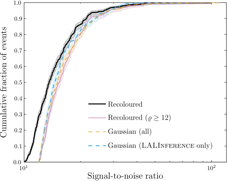
The recoloured SNR distribution includes a tail at low SNR ($\varrho\simeq 10$–$12$). If we impose a lower threshold $\varrho\geq 12$ for the recoloured data set, as was done for the Gaussian data set, we find that the SNR distributions are similar. With the shared SNR cut, the distributions agree within the expected sampling error; performing a Kolmogorov–Smirnov (KS) test (DeGroot:1975, section 9.5) comparing the recoloured SNR distribution to the complete (LALInference only) Gaussian SNR distribution returns a $p$-value of $0.311$ ($0.110$).

Comparing injections between the recoloured and Gaussian data sets, there are $255$ events that have been detected in both sets. There are $108$ events shared between the recoloured data set and the sub-sample of the Gaussian data set analysed with LALInference. Considering individual events, we may contrast the SNR for recoloured noise $\varrho_{\mathrm{R}}$ and Gaussian noise $\varrho_{\mathrm{G}}$. The ratio of the two SNRs n figure 3.

Figure 3.— Comparison of rom injections with Gaussian noise $\varrho_{\mathrm{G}}$ and from injections with recoloured noise $\varrho_{\mathrm{R}}$. (a) The ratio $\varrho_{\mathrm{R}}/\varrho_{\mathrm{G}}$ as a function of $\varrho_{\mathrm{G}}$. The dashed line shows the locus of $\varrho_{\mathrm{R}}=12$. (b) Distribution of $\varrho_{\mathrm{R}}/\varrho_{\mathrm{G}}$ with both $\varrho_{\mathrm{G}}\geq 12$ and $\varrho_{\mathrm{R}}\geq 12$, using a bin width of $0.5$. Events that fall within the sub-sample of Gaussian events analysed with LALInference are highlighted with blue (star-shaped points) and the complete set of events detected in both the Gaussian and recoloured data sets is indicated by orange (round points).

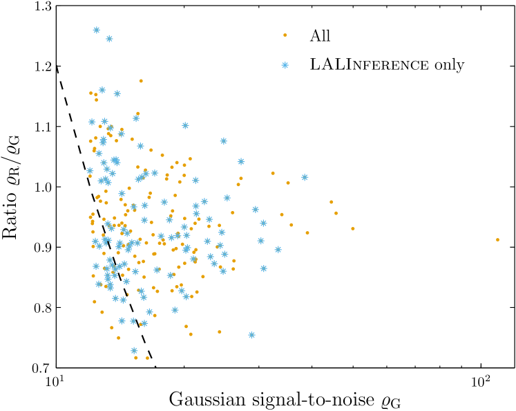
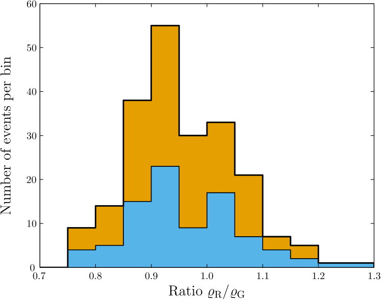
Considering the entire population of shared detections, the mean value of the ratio of SNRs is $\varrho_{\mathrm{R}}/\varrho_{\mathrm{G}}=0.938\pm 0.006$, showing a small downwards bias as an effect of the differing cutoffs used for the two samples. To limit selection effects that could skew the distribution of the ratio of SNRs, we can impose an SNR cut of $\varrho_{\mathrm{R}}\geq 12$. This reduces the number of events detected in both noise sets to $214$ using the full Gaussian set and $88$ for the LALInference Gaussian sub-sample. There is a small difference between the SNR as calculated with Gaussian noise and with recoloured noise. This does not appear to be a strong function of the SNR. However, the scatter in the ratio decreases as SNR increases, approximately decreasing as $\varrho^{-1}$. This is as expected as the inclusion of random noise realisations in the signal should produce fluctuations in the SNR of order $\pm 1$; these fluctuations become less significant for louder events. After imposing the cut $\varrho\geq 12$ on both sets, the mean value of the ratio of SNRs is $\varrho_{\mathrm{R}}/\varrho_{\mathrm{G}}=0.955\pm 0.006$. Although there is a small difference in SNRs, we shall see that this does not impact our PE results.

4.1.2 Selection effects

The population of detected events should not match exactly the injected distribution; depending upon their parameters, some systems are louder and hence easier to detect. Here, we look at the selection effects of the most astrophysically interesting parameters: mass and spin. We expect there to be a selection based upon mass, as the component masses set the amplitude of the waveform. We do not expect there to be a dependence upon the spin because the spin magnitude is small, but since we injected with a spinning waveform and recovered with a non-spinning waveform, there could potentially be a selection effect due to waveform mismatch. Checking these distributions confirms the effectiveness of the detection pipeline for this study.

To leading order, the GW amplitude is determined by the ($5/6$ power of the) chirp mass (Sathyaprakash:2009xs)

$$\mathcal{M}_{\mathrm{c}}=\frac{(m_{1}m_{2})^{3/5}}{(m_{1}+m_{2})^{1/5}},$$ (1)

where $m_{1}$ and $m_{2}$ are the individual component masses. We therefore expect to preferentially select systems with larger chirp masses.

Figure 4 shows the recovered distribution of (injected) chirp masses and the injection distribution (which is calculated numerically).

Figure 4.— Cumulative fractions of detected events with chirp masses smaller than the abscissa value. Results using recoloured noise are denoted by the solid line, and results from the subset of $250$ events with Gaussian noise analysed with LALInference are denoted by the dashed line (Singer:2014qca). The $68\%$ confidence intervals are denoted by the shaded areas. The injection distribution, based upon a uniform distribution of component masses, is indicated by the dot–dashed line.

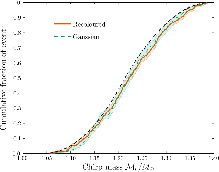
We do detect fewer systems with smaller chirp masses (and more with larger chirp masses), as indicated by the curve for the recovered distribution lying below the curve for the injection distribution. However, this selection effect does not alter the overall character of population. The difference is only marginally statistically significant with this number of events (a KS test with the injection distribution yields $p$-values of $0.315$ and $0.068$ for the Gaussian and recoloured noise respectively). This is consistent with expectations for this narrow chirp-mass distribution; in appendix LABEL:ap:mass we use a simple theoretical model to predict that we would need $\sim 10^{3}$ detections (or a broader distribution of chirp masses in the injection set) to see a significant difference between the injected and recovered populations. The character of the noise does not influence the chirp-mass distribution (a KS test gives a $p$-value of $0.999$).

For completeness, in appendix LABEL:ap:mass we present the distributions for the individual component masses, the asymmetric mass ratio and the total mass. The selection effects on these depend upon their correlation with the chirp mass; the total mass, which is most strongly correlated with the chirp mass, shows the most noticeable difference between injection and detected distributions.

Since we injected with a spinning waveform and recovered with a non-spinning waveform, there could also be a selection bias depending upon the spin magnitude. Figure 5 shows the recovered distribution of (injected) spins.

Figure 5.— Cumulative fractions of detected events with spin magnitudes smaller than the abscissa value. The spin distribution for the first neutron star $a_{1}$ is denoted by the solid line, and the distribution for the second neutron star $a_{2}$ is denoted by the dashed line. Results using recoloured noise are denoted by the thicker red–purple lines, and results from the subset of $250$ events with Gaussian noise analysed with LALInference are denoted by the thinner blue–green lines (Singer:2014qca). The $68\%$ confidence intervals are denoted by the shaded areas. The expected distribution for spins uniform from $a_{\mathrm{min}}=0$ to $a_{\mathrm{max}}=0.05$ is indicated by the black dot–dashed line.

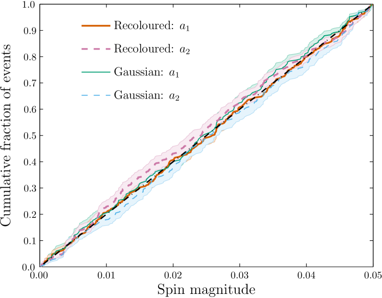
The detected events are consistent with having the uniform distribution of spins used for the injections. in agreement with Brown:2012qf.

4.2. Sky-localization accuracy

The recovered sky positions from bayestar and LALInference appear in good agreement. A typical example of the recovered posterior probability density is shown in figure LABEL:fig:sky-map.

(a)

(b)

Figure 6.— Posterior probability density for sky location, plotted in a Mollweide projection in geographic coordinates. The star indicates the true source location. (a) Computed by bayestar. (b) Computed by LALInference. The event has simulation ID 1243 and a network SNR of $\varrho=13.2$. fig:sky-map

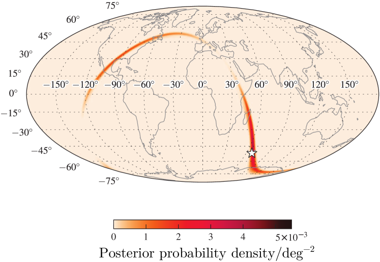
This is a bimodal distribution, reflecting the symmetry in the sensitivity of the detectors, which is common (Singer:2014qca). We use geographic coordinates to emphasise the connection to the position of the detectors. To quantify the accuracy of sky localization, we use credible regions: areas of the sky that include a given total posterior probability. We denote the credible region for a total posterior probability $p$ as $\mathrm{CR}_{p}$: it is defined as

$$\mathrm{CR}_{p}\equiv\min{A}$$ (2)

such that the sky area $A$ satisfies

$$p=\int_{A}\mathrm{d}\boldsymbol{\Omega}P_{\Omega}(\boldsymbol{\Omega}),$$ (3)

where $P_{\Omega}(\boldsymbol{\Omega})$ is the posterior probability density over sky position $\boldsymbol{\Omega}$ (Sidery:2013zua). A smaller $\mathrm{CR}_{p}$ at a given $p$ indicates more precise sky localization.

We also consider the searched area: the area of the smallest credible region that includes the true location, and, hence, the area of the sky that we expect would have to be observed before the true source was found.

The self-consistency of our sky areas can be checked by calculating the fraction of events that fall within the credible region at the given probability. We expect that a fraction $p$ of true sky positions are found within $\mathrm{CR}_{p}$; that is the frequentist confidence region agrees with our Bayesian credible region (Sidery:2013zua). Figure 7 shows the fraction of events found within a given $\mathrm{CR}_{p}$ as a function of $p$.

Figure 7.— Fraction of true locations found within a credible region as a function of encompassed posterior probability. Results from LALInference are indicated by the solid line, results from bayestar are indicated by the dashed line and the expected distribution is indicated by the dot–dashed diagonal line. The $68\%$ confidencee interval is enclosed by the shaded regions, this accounts for sampling errors and is estimated from a beta distribution (Cameron:2010bh).

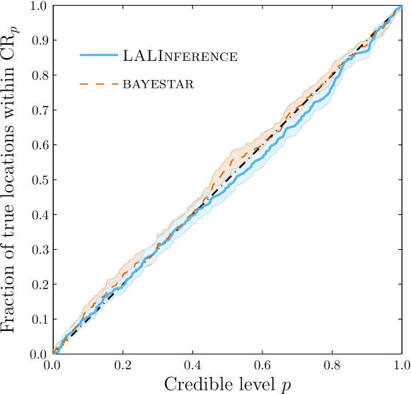
The distributions are consistent with expectations: performing a KS test with the predicted distribution yields $p$-values of $0.455$ and $0.546$ for LALInference and bayestar respectively. Both LALInference and bayestar produce self-consistent and unbiased sky areas in the presence of recoloured noise.

The recovered sky areas are plotted in figure 8. This shows the cumulative distribution of areas for $\mathrm{CR}_{0.5}$, $\mathrm{CR}_{0.9}$ and searched areas $A_{\ast}$ as recovered from LALInference and bayestar. oth the results using recoloured noise and the results using Gaussian noise from Singer:2014qca.

Figure 8.— Cumulative fractions of events with sky-localization areas smaller than the abscissa value. (a) Sky area of $50\%$ credible region $\mathrm{CR}_{0.5}$, the (smallest) area enclosing $50\%$ of the total posterior probability. (b) Sky area of $\mathrm{CR}_{0.9}$. (c) Searched area $A_{\ast}$, the area of the smallest credible region containing the true position. LALInference and bayestar results are denoted by thicker blue and thinner red–orange lines respectively. The results of this study are indicated by a solid line, while the results of Singer:2014qca, which uses Gaussian noise, are indicated by a dashed line. The $68\%$ confidence intervals are denoted by the shaded areas.

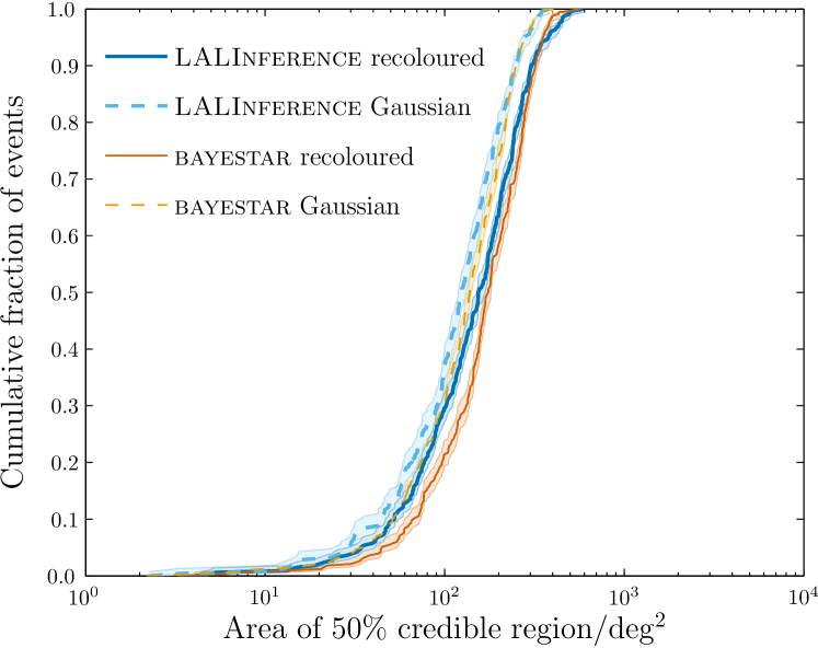
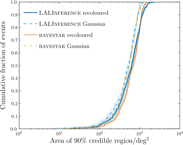
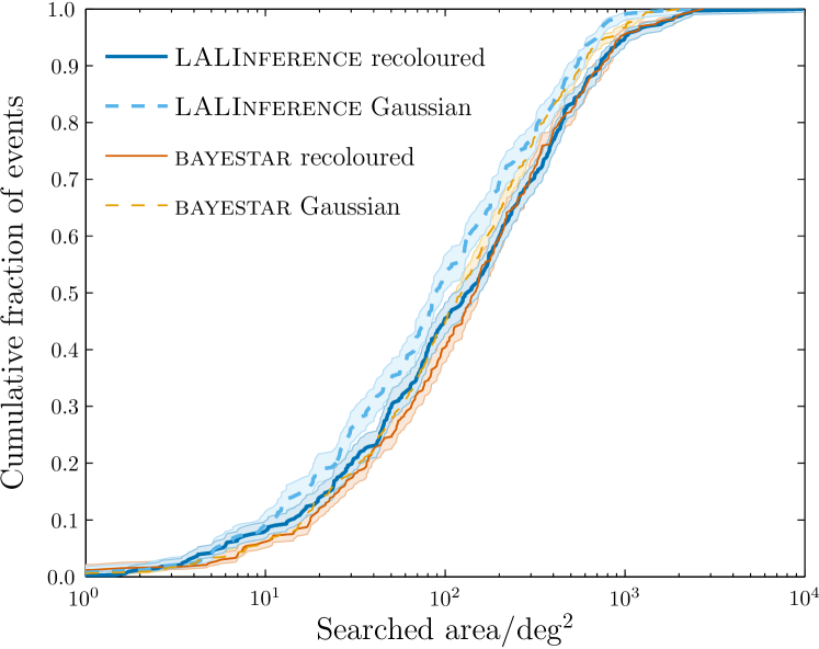
All the results are similar. LALInference produces (marginally) more accurate sky localizations than bayestar, but the rapid code does a successful job of reconstructing the sky position in a much shorter time (see appendix LABEL:ap:cost for estimates of computation time). The recovered areas are (generally) marginally smaller for LALInference as this makes use of more information and so is expected to perform better (a KS test returns $p$-values of $0.740$ when comparing $\mathrm{CR}_{0.9}$ for Gaussian noise and $0.181$ for recoloured noise).

The difference between the Gaussian and recoloured results can be understood as a consequence of the SNR distribution (see figure 2). The SNR is the dominant factor affecting sky localization. For example, there is no strong correlation between the time delay between detection at the two LIGO sites and the sky-localization accuracy. The inclusion of more low-SNR events means that, on average, the results using recoloured noise are worse.

The sky-localization accuracy is expected to scale The uncertainty in each direction on the sky scales inversely with the SNR, hence the area scales inversely with the square of the SNR (cf. Fairhurst:2009tc; Fairhurst:2010is). This SNR scaling can be verified by plotting recovered sky areas as a function of $\varrho$ as shown in figure 4.2.

Figure 9.— Sky-localization areas as a function of ϱ$.(a)Skyareaof$50%$credibleregion$CR_0.5$.(b)Skyareaof$CR_0.9$.Individualresultsareindicatedbypoints.Weincludesimplebest-fitlinesassumingthatthearea$A ∝ϱ^-2$.\textsc{LALInference}and\textsc{bayestar}resultsaredenotedbythickerblueandthinnerred--orangelinesrespectively.Theresultsofthisstudyareindicatedbyasolidline,whiletheresultsof\cite[citet]{\@@bibref{Authors Phrase1YearPhrase2}{Singer:2014qca}{\@@citephrase{(}}{\@@citephrase{)}}},whichusesGaussiannoise,areindicatedbyadashedline.$

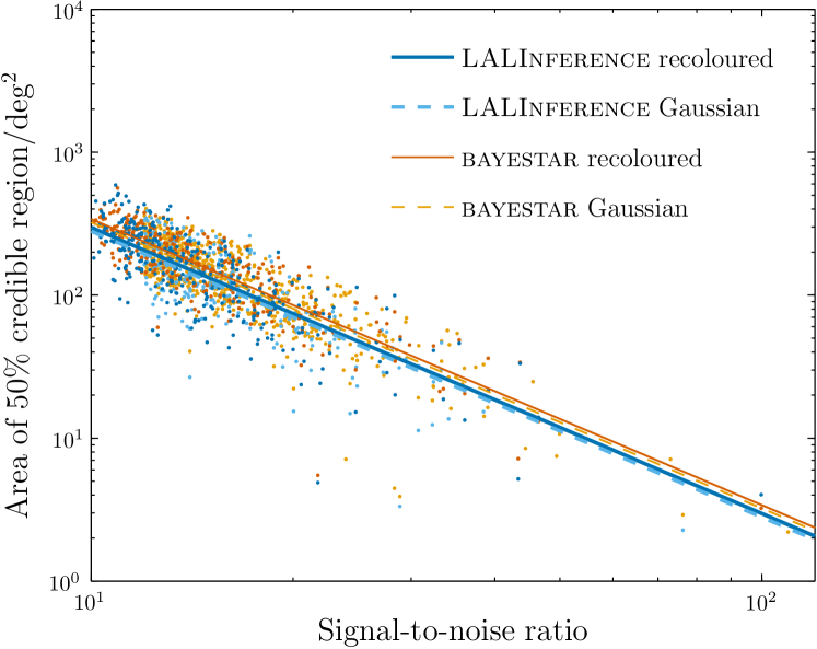
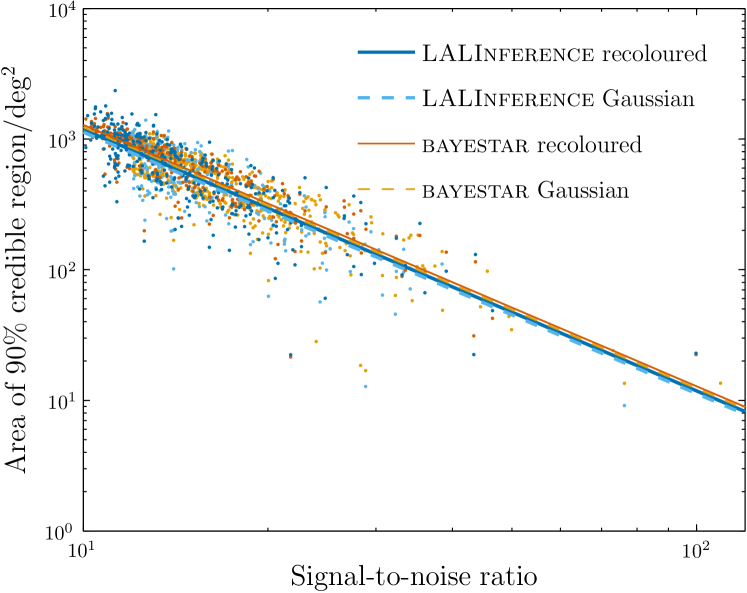
The recovered areas do show the expected correlation, although there is considerable scatter resulting from the variation in intrinsic parameters.

We have plotted fiducial best-fit lines with the expected scaling. The fitting was done simply using a naive least-squares method, fitting a straight line to $\log\varrho$ and $\log A$ for each sky area $A$. Allowing the slope of the line to vary from $-2$ yields negligible change to the fit. There is little difference between the trends for the recoloured and Gaussian results, indicating that the variation in the sky-localization accuracies is primarily an effect of the different distribution of SNRs. There is a small discrepancy between LALInference and bayestar in both cases, but the difference is not significant and is within the uncertainty expected from the scatter of results. The general trend for the sky-localization areas can be approximated as

$$\log_{10}\left(\frac{\mathrm{CR}_{0.5}}{\mathrm{deg^{2}}}\right)\approx{} -2\log_{10}\varrho+4.46,$$ (4a)

$$\log_{10}\left(\frac{\mathrm{CR}_{0.9}}{\mathrm{deg^{2}}}\right)\approx{} -2\log_{10}\varrho+5.06.$$ (4b)

Sky-localization accuracy (at a given SNR) does not appear to be sensitive to the Gaussianity of the noise.

From our fits (4), we can immediately see that the ratio $\mathrm{CR}_{0.9}/\mathrm{CR}_{0.5}$ is about $10^{0.6}\simeq 4$. Considering this ratio for each posterior, the mean value of $\log_{10}(\mathrm{CR}_{0.9}/\mathrm{CR}_{0.5})$ is $0.60$ and the standard deviation is $0.07$. For comparison, if the posterior were a $1$-d Gaussian, we would expect the ratio to be $\operatorname{erf}^{-1}(0.9)/\operatorname{erf}^{-1}(0.5)\simeq 2.4\simeq 10^{0.39}$, and if it were a $2$-d Gaussian, the ratio would be $\ln(1-0.9)/\ln(1-0.5)\simeq 3.3\simeq 10^{0.52}$ (Fairhurst:2009tc; Fairhurst:2010is). Neither of these agree well. The sky-location posteriors can have complicated shapes, and cannot be accurately modelled by a simple Gaussian description.

To verify that SNR distribution is the dominant cause of difference between the Gaussian and recoloured results, we impose a cut on the recoloured data set of $\varrho\geq 12$ to match the Gaussian set. This reduces the number of events from $333$ to $236$. The cumulative distribution of sky-localization areas for results with $\varrho\geq 12$ are shown in figure 10.

Figure 10.— Cumulative fractions of events with sky-localization areas smaller than the abscissa value as in figure 8 but imposing an SNR cut of $\varrho_{\mathrm{R}}\geq 12$. (a) Sky area of $\mathrm{CR}_{0.5}$. (b) Sky area of $\mathrm{CR}_{0.9}$. (c) Searched area $A_{\ast}$. LALInference and bayestar results are denoted by thicker blue and thinner red–orange lines respectively. The results of this study are indicated by a solid line, while the results of Singer:2014qca, which uses Gaussian noise, are indicated by a dashed line. The $68\%$ confidence intervals are denoted by the shaded areas.

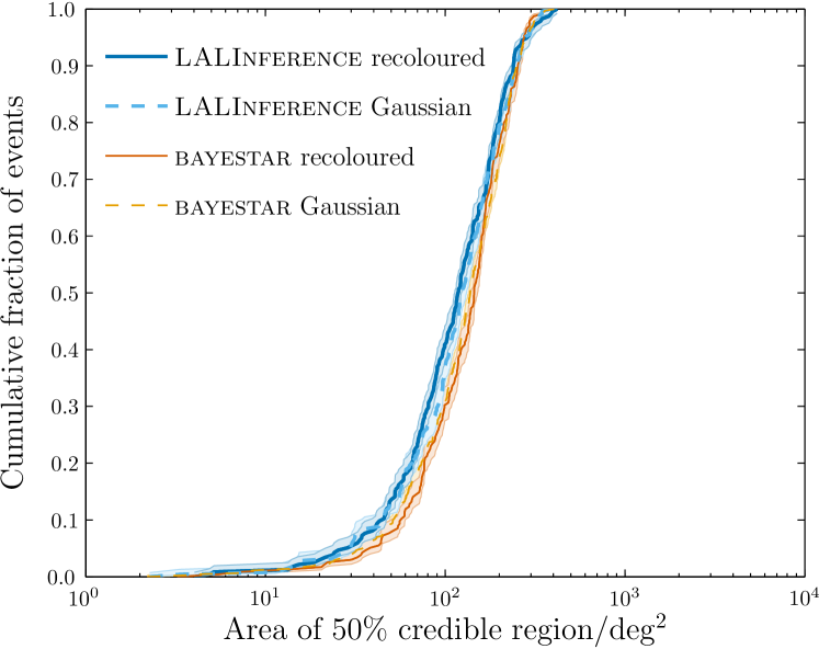
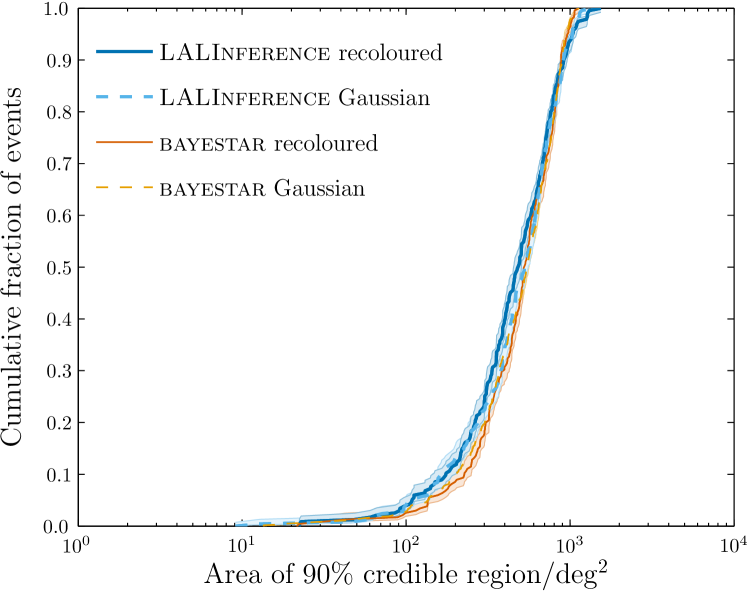
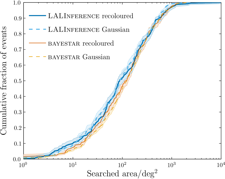
The distributions do overlap as expected: the Gaussian and recoloured results are in agreement (a KS test on $\mathrm{CR}_{0.9}$ gives a $p$-value of $0.550$ when comparing LALInference results between noise realizations and $0.673$ for bayestar).

The key numbers describing the distributions are given in tables 1 and 2; the former gives the fraction of events with sky-localization areas smaller than fiducial values, and the latter gives median sky-localization areas. Our results are discussed further in section LABEL:sec:ob-scenario.

Table 1Fractions of events with sky-localization areas smaller than a given size from this study using recoloured noise and Singer:2014qca, which uses Gaussian noise. Results are quoted for the full catalogue of results with recoloured noise and imposing a SNR cut of $\varrho\geq 12$ to match the Gaussian catalogue. Figures for the $50\%$ credible region $\mathrm{CR}_{0.5}$, the $90\%$ credible region $\mathrm{CR}_{0.9}$ and the searched area $A_{\ast}$ are included. A dash (—) is used for fractions less than $0.01$.

		Gaussian noise		Recoloured noise		Recoloured noise $\varrho\geq 12$
		bayestar	LALInference	bayestar	LALInference	bayestar	LALInference
$\mathrm{CR}_{0.5}\leq$	$5~{}\mathrm{deg^{2}}$	—	—	—	—	—	—
	$20~{}\mathrm{deg^{2}}$	$0.02$	$0.03$	$0.01$	$0.02$	$0.02$	$0.03$
	$100~{}\mathrm{deg^{2}}$	$0.30$	$0.37$	$0.21$	$0.30$	$0.30$	$0.41$
	$200~{}\mathrm{deg^{2}}$	$0.74$	$0.80$	$0.58$	$0.64$	$0.76$	$0.80$
	$500~{}\mathrm{deg^{2}}$	$1.00$	$1.00$	$1.00$	$0.99$	$1.00$	$1.00$
	$1000~{}\mathrm{deg^{2}}$	$1.00$	$1.00$	$1.00$	$1.00$	$1.00$	$1.00$
$\mathrm{CR}_{0.9}\leq$	$5~{}\mathrm{deg^{2}}$	—	—	—	—	—	—
	$20~{}\mathrm{deg^{2}}$	—	—	—	—	—	—
	$100~{}\mathrm{deg^{2}}$	$0.03$	$0.04$	$0.02$	$0.03$	$0.03$	$0.04$
	$200~{}\mathrm{deg^{2}}$	$0.10$	$0.13$	$0.06$	$0.08$	$0.09$	$0.12$
	$500~{}\mathrm{deg^{2}}$	$0.44$	$0.48$	$0.31$	$0.38$	$0.44$	$0.52$
	$1000~{}\mathrm{deg^{2}}$	$0.98$	$0.93$	$0.78$	$0.80$	$0.96$	$0.94$
$A_{\ast}\leq$	$5~{}\mathrm{deg^{2}}$	$0.03$	$0.04$	$0.03$	$0.04$	$0.03$	$0.06$
	$20~{}\mathrm{deg^{2}}$	$0.14$	$0.19$	$0.12$	$0.14$	$0.15$	$0.16$
	$100~{}\mathrm{deg^{2}}$	$0.45$	$0.54$	$0.40$	$0.45$	$0.47$	$0.52$
	$200~{}\mathrm{deg^{2}}$	$0.64$	$0.70$	$0.60$	$0.60$	$0.66$	$0.68$
	$500~{}\mathrm{deg^{2}}$	$0.87$	$0.89$	$0.82$	$0.83$	$0.87$	$0.89$
	$1000~{}\mathrm{deg^{2}}$	$0.97$	$0.99$	$0.96$	$0.95$	$0.98$	$0.97$

Table 2Median sky-localization areas from this study using recoloured noise, and Singer:2014qca, which uses Gaussian noise. Results are quoted for the full catalogue of results with recoloured noise and imposing a SNR cut of $\varrho\geq 12$ to match the Gaussian catalogue. Figures for the $50\%$ credible region $\mathrm{CR}_{0.5}$, the $90\%$ credible region $\mathrm{CR}_{0.9}$ and the searched area $A_{\ast}$ are included.

		Gaussian noise		Recoloured noise		Recoloured noise $\varrho\geq 12$
		bayestar	LALInference	bayestar	LALInference	bayestar	LALInference
Median	$\mathrm{CR}_{0.5}$	$138~{}\mathrm{deg^{2}}$	$124~{}\mathrm{deg^{2}}$	$175~{}\mathrm{deg^{2}}$	$154~{}\mathrm{deg^{2}}$	$145~{}\mathrm{deg^{2}}$	$118~{}\mathrm{deg^{2}}$
	$\mathrm{CR}_{0.9}$	$545~{}\mathrm{deg^{2}}$	$529~{}\mathrm{deg^{2}}$	$692~{}\mathrm{deg^{2}}$	$632~{}\mathrm{deg^{2}}$	$524~{}\mathrm{deg^{2}}$	$481~{}\mathrm{deg^{2}}$
	$A_{\ast}$	$123~{}\mathrm{deg^{2}}$	$\hphantom{0}88~{}\mathrm{deg^{2}}$	$145~{}\mathrm{deg^{2}}$	$132~{}\mathrm{deg^{2}}$	$118~{}\mathrm{deg^{2}}$	$\hphantom{0}88~{}\mathrm{deg^{2}}$

4.3. Mass and distance estimation

Independent of any EM counterpart, GW astronomy is still informative. GW observations allow for measurement of various properties of the source system. Here, we examine the ability to measure luminosity distance and mass (principally the chirp mass of the system).

Accurate mass and distance measurements have many physical applications. Measurement of the chirp-mass distribution can constrain binary evolution models (Bulik:2003ap). Determining the maximum mass of a neutron star would shed light on its equation of state (e.g., Read:2009yp), and, potentially, on the existence of a mass gap between neutron stars and black holes (Ozel:2010; Farr:2010; Kreidberg:2012ud). Combining mass and distance measurement, it may be possible to construct a new (independent) measure of the Hubble constant (Taylor:2011fs). GW observations shall give us unique insight into the properties of BNS systems.

In addition to component masses and the distance to the source, the component spins are of astrophysical importance (e.g., Mandel:2009nx). Unfortunately, we cannot estimate the component spins as we are using non-spinning waveform templates. Measurement of the spins will be examined in a future study investigating PE using SpinTaylorT4 waveforms.

4.3.1 Luminosity distance

Quantifying the precision of distance estimation is simpler than for sky localization as we are now working in a single dimension. The equivalent of a credible region is a credible interval. We denote the distance credible interval for a total posterior probability $p$ as $\mathrm{CI}^{D}_{p}$. It is defined to exclude equal posterior probabilities in each of the tails; it is given by

$$\mathrm{CI}^{D}_{p}=C^{-1}_{D}\left(\frac{1+p}{2}\right)-C^{-1}_{D}\left(\frac{1-p}{2}\right),$$ (5)

where $C^{-1}_{D}(p)$ is the inverse of the cumulative distribution function

$$C_{D}(D)=\int_{0}^{D}\mathrm{d}D^{\prime}P_{D}(D^{\prime})$$ (6)

for distance posterior $P_{D}(D)$. The same symmetric definition for the credible interval was used by Aasi:2013jjl. A smaller $\mathrm{CI}^{D}_{p}$ for a given $p$ indicates more precise distance estimation.

The self-consistency of our distance estimates can be verified by calculating the fraction of true values that fall within the credible interval at a given $p$. This is shown in figure 11 for results from both the Gaussian and recoloured noise results.

Figure 11.— Fraction of true luminosity distances found within a credible interval as a function of encompassed posterior probability. Results using recoloured noise are indicated by a solid line, while the results using Gaussian noise (Singer:2014qca) are indicated by a dashed line. The expected distribution is indicated by the dot–dashed diagonal line. The shaded regions enclose the $68\%$ confidence intervals accounting for sampling errors.

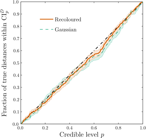
Both distributions are consistent with expectations (performing a KS test with the predicted distribution yields $p$-values of $0.168$ and $0.057$ for the recoloured and Gaussian noise respectively). LALInference does return self-consistent distance estimates.

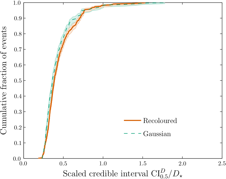
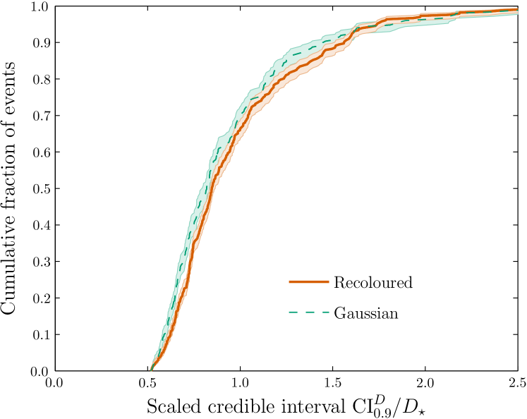
The cumulative distributions of credible intervals are plotted in figure 12. We divide the credible interval by the true (injected) distance $D_{\star}$; this gives an approximate analogue of twice the fractional uncertainty.

Figure 12.— Cumulative fractions of events with luminosity-distance credible intervals (divided by the true distance) smaller than the abscissa value. (a) Scaled $50\%$ credible interval $\mathrm{CI}^{D}_{0.5}/D_{\star}$. (b) Scaled $90\%$ interval $\mathrm{CI}^{D}_{0.9}/D_{\star}$. Results using recoloured noise are indicated by a solid line and the results using Gaussian noise (Singer:2014qca) are indicated by a dashed line. The $68\%$ confidence intervals are denoted by the shaded areas.

The CI^D_p/D_⋆$appearsinsensitivetothedetectioncut-off(aKStestbetween$CI^D_0.9/D_⋆$fortherecolouredandGaussianresultsgivesa$p$-valueof$0.077$).Thisappearsincontrasttothecaseforskyareas,butthedifferingSNRdistributionsareaccountedforbyscalingwithrespecttothedistance(whichisinverselyproportionaltotheSNR).Theestimationofthedistance,likethatforskyareas,doesnotdependuponthecharacterofthenoise.\par Distanceestimationisimprecise:theposteriorwidthsarefrequentlycomparablethethemagnitudeofthedistanceitself.Thisisaconsequenceofadegeneracybetweenthedistanceandtheinclination\cite[citep]{(\@@bibref{AuthorsPhrase1Year}{Cutler:1994ys,Aasi:2013jjl}{\@@citephrase{, }}{})}.Thekeynumberssummarisingdistanceestimationaregivenintables\ref{tab:fraction-dist}and\ref{tab:median-dist};theformergivesthefractionofeventswith$CI^D_p/D_⋆$smallerthanfiducialvalues,andthelattergivesmedianvalues.\text{Table 3Table 33Table 33Fractionsofeventswithfractionaldistanceest}$