Keeping it real: revisiting a real-space approach to running ensembles of cosmological N-body simulations

Abstract

In setting up initial conditions for ensembles of cosmological N-body simulations there are, fundamentally, two choices: either maximizing the correspondence of the initial density field to the assumed fourier-space clustering or, instead, matching to real-space statistics and allowing the DC mode (i.e. overdensity) to vary from box to box as it would in the real universe. As a stringent test of both approaches, I perform ensembles of simulations using power law and a “powerlaw times a bump” model inspired by baryon acoustic oscillations (BAO), exploiting the self-similarity of these initial conditions to quantify the accuracy of the matter-matter two-point correlation results. The real-space method, which was originally proposed by Pen 1997 [1] and implemented by Sirko 2005 [2], performed well in producing the expected self-similar behavior and corroborated the non-linear evolution of the BAO feature observed in conventional simulations, even in the strongly-clustered regime ($\sigma_{8}\gtrsim 1$). In revisiting the real-space method championed by [2], it was also noticed that this earlier study overlooked an important integral constraint correction to the correlation function in results from the conventional approach that can be important in $\Lambda$CDM simulations with $L_{\rm box}\lesssim 1\,h^{-1}$Gpc and on scales $r\gtrsim L_{\rm box}/10$. Rectifying this issue shows that the fourier space and real space methods are about equally accurate and efficient for modeling the evolution and growth of the correlation function, contrary to previous claims. An appendix provides a useful independent-of-epoch analytic formula for estimating the importance of the integral constraint bias on correlation function measurements in $\Lambda$CDM simulations.

1 Introduction

Next-generation astronomical surveys will demand increasingly precise predictions from theory in order to properly interpret observations and constrain the nature of dark energy. As emphasized by [3, 4], this will be a challenging task: inaccuracies in the predictions of halo abundance and halo bias, for example, can affect cosmological inferences [6, 5], and measurements of the baryon acoustic oscillations (BAO) clustering feature will soon reach the stage where theoretical estimates of the shift of this feature from non-linear dynamics become important [7]. Although current state-of-the-art cosmological N-body simulations, given a specific set of cosmological parameters, are in many ways well-equipped to deliver highly precise predictions of the dark matter two-point correlation function and power spectrum for a relatively wide range of scales [8], the difficult-to-estimate covariances of these statistics are also crucial for placing constraints on cosmological parameters [9, 10]. While much creativity has gone into methods and algorithms that ultimately save substantial computer time in delivering these predictions [11, 12, 13, 14] the cosmological $N$-body simulations that these methods draw upon, with very few exceptions, are conducted without allowing the overdensity in each box to vary as it would if boxes of a cosmologically-relevant size were randomly positioned in the universe. The goal of this paper is twofold: (1) to assess the ramifications of this choice and in doing so explore the predictions of the conventional (or “standard”) method, (2) to explore the predictions of a method that does allow the overdensity to vary from box-to-box or otherwise to document – for lack of existing references – why the field has largely abandoned this approach.

Since other authors have adequately described the conventional method [15, 16, 17], which seeks to maximize the correspondence between the assumed initial fourier space clustering properties in the simulation and the fourier-space properties of the assumed cosmological model, I here focus the discussion on a method for running ensembles of simulations that is designed to instead maximize the correspondence between simulated real-space clustering statistics (e.g. $\sigma_{8},\xi(r)$) and the real-space properties of the assumed cosmological model. Originally proposed by Pen [1] and implemented by Sirko [2], as this method allows the so-called DC mode of each simulation (in an ensemble of simulations) to vary self-consistently according to the clustering power on the scale of the box in much the same way that the density within randomly placed boxes in the real universe will fluctuate around the mean density. In the early days of fully cosmological $N$-body simulations [e.g. 18] this effect was sometimes included, albeit in less-sophisticated ways than in [1] and [2].

In the Sirko [2] framework the initial power spectrum used with the Zeldovich [21] (and by extension 2LPT [22, 23]) approximation is convolved such that the matter correlation function matches exactly the linear theory correlation function for $r<L_{\rm{box}}/2$, while for $r>L_{\rm{box}}/2$ the correlation function is set to zero. With this in mind Sirko refers to this approach as “$\xi$-sampled” initial conditions (ICs), while the standard method is referred to as “$P$-sampled”, since by using an unconvolved linear theory power spectrum with the Zeldovich approximation the initial conditions are instead matched to the fourier space clustering statistics. The $\xi$-sampled strategy, by matching the correlation function out to $r=L_{\rm{box}}/2$, should avoid biases on all real space statistics, since the rms overdensity in spheres, $\sigma(R)$, is simply related to the correlation function, and the halo mass function to good approximation is only a function of $\sigma(R)$ [24, 25, 26]. Without this convolution these real space statistics become biased (e.g. from $P(k)=0$ for $k\lesssim 2\pi/L_{\rm{box}}$), as discussed by [1] and [27]. Sirko [2] presents a set of $\Lambda$CDM simulations with 100$h^{-1}$ Mpc box sizes that indicate that the conventional, $P$-sampled method can give strongly biased results for the matter correlation function on scales near 1/4th the size of the box, independently of epoch, while the results of $\xi$-sampled simulations with the same parameters give much more reasonable matter correlation functions on these scales. This conclusion is revisited in § 3, which argues that if a measurement-bias correction is applied to the $P$-sampled results, the two methods are consistent.

Although a number of groups have published results using the initial conditions code developed by Sirko, which was the among the first include the 2nd order Lagrangian corrections [22, 23] to the Zeldovich [21] displacements, the code is very seldom used to generate $\xi$-sampled ICs. To my knowledge, only Reid et al. [28] have utilized the code in this mode, citing the success of convergence tests in [29]. In that study they create mock catalogues from a suite of 42 simulations with $L_{\rm{box}}=558h^{-1}$ Mpc, and $N=512^{3}$ for comparison with SDSS LRG data [30]. They chose the $\xi$-sampled method for this task, citing the attractive feature of allowing the DC mode of the box to vary, thereby modeling the power spectrum covariance of real surveys more realistically. [29] and Appendix A of [28] present a wide variety of convergence tests that explore the effects of increasing the resolution with either fixed initial conditions (i.e. with a particular randomly sampled value for the DC mode) or for a set of a few initial conditions realizations. More recently, [31] argued that the DC mode should be re-introduced and compared the results of five $L_{\rm{box}}=20h^{-1}$ Mpc, $\Lambda$CDM simulations using the $\xi$-sampled method to a high-resolution, standard-method simulation with $L_{\rm{box}}=80h^{-1}$ Mpc, finding good correspondence between the results for the variance of the halo mass function.

This study systematically explores the predictions of the two different methods using relatively large ensembles of simulations (20 unless otherwise noted) and a diverse set of initial conditions. Where the results disagree it may be ambiguous which approach is more accurate, therefore I focus on pure powerlaw models which should evolve self-similarly. This allows highly-accurate self-consistency checks of the simulation results, since each output should, in a statistical sense, resemble scaled versions of earlier and later outputs. These kinds of “self-similar” tests were decisive in confirming the accuracy of the first generation of fully cosmological N-body codes [32]. I also show a few tests where, instead of a pure powerlaw, I simulate BAO-inspired initial conditions consistent with a configuration space powerlaw times a gaussian bump. Investigated in great depth in [33] using the conventional method, this test is self-similar in a different sense – namely that the evolution of the dark matter clustering should only depend on the ratio of the scale of non-linearity to the scale of the BAO. I include these initial conditions as another test of the $\xi$-sampled method and as a valuable cross-check for the conventional method’s predictions for the non-linear evolution of the BAO feature. Importantly, these simulations can explore the shift and broadening of the BAO bump even in the strongly-clustered regime ($\sigma_{8}\gtrsim 1$).

I test these models extensively, focusing on pure powerlaw models with spectral slopes of $n=-1$, $-1.5$, and $-2$, and on the three models explored in [33] which resemble $n=-0.5$, $-1$, and $-1.5$ powerlaws in fourier space. § 2 gives an overview of the $\xi$-sampled method. § 3 describes aspects of measuring the correlation function in $\xi$-sampled and $P$-sampled simulations, including the importance of the integral constraint measurement bias which led Sirko [2] to believe incorrectly that correlation functions in $P$-sampled, $\Lambda$CDM simulations are suppressed for $r\gtrsim L_{\rm box}/10$. § 4 describes powerlaw initial conditions in the $\xi$-sampled context. I compare predictions from the two methods, showing results for the matter-matter two-point correlation function in § 5. In § 6 I investigate results for the variance of the correlation function, comparing the results from the two methods to each other and to expectations from theory. In § 7 I summarize my main conclusions. Appendix A presents a simple, independent-of-epoch analytic formula that, given the box size, can estimate the importance of the integral constraint in $\Lambda$CDM simulations.

2 Overview of the $\xi$-sampled Method

In the $\xi$-sampled method implemented by [2], the (real space) matter correlation function for a given cosmological model is the (usual) fourier transform of the power spectrum

$$\xi(r)=\int\frac{d^{3}k}{(2\pi)^{3}}P(k)\,e^{i\vec{k}\cdot\vec{r}}=\frac{1}{2\pi^{2}}\int_{0}^{\infty}P(k)\,\frac{\sin kr}{kr}\,k^{2}\,{dk}.$$ (2.1)

To convolve $P(k)$ such that the simulated $\xi(r)$ is an exact match to Eq. 2.1 for $r<L_{\rm{box}}/2$, but is zero for larger separations, one simply fourier transforms $\xi(r)$ while cutting off the integral at $L_{\rm{box}}/2$ since $\xi(r)=0$ for $r>L_{\rm{box}}/2$,

$$P_{\rm{real}}(k)=4\pi\int_{0}^{L_{\rm{box}}/2}\xi(r)\,\frac{\sin kr}{kr}\,r^{2}\,{dr}.$$ (2.2)

I will refer to this result as $P_{\rm{real}}(k)$ to emphasize that this power spectrum is designed to maintain correspondence with the real space properties of the cosmological density field. Importantly, $P_{\rm{real}}(0)$ can be non-zero even if $P(0)=0$; this term sets the fluctuations in the DC mode. In Appendix A of [2], using the subscript “uni” to denote variables in the model of interest and “box” to identify the parameters of the simulated volume, these fluctuations are mapped self-consistently onto fluctuations in cosmological parameters,

$$H_{0,\rm{box}}=H_{0,\rm{uni}}\frac{1}{1+\phi},$$ (2.3)

$$\Omega_{m,\rm{box}}=\Omega_{m,\rm{uni}}(1+\phi)^{2},$$ (2.4)

$$\Omega_{\Lambda,\rm{box}}=\Omega_{\Lambda,\rm{uni}}(1+\phi)^{2},$$ (2.5)

$$\phi=\frac{5}{6}\frac{\Omega_{m}}{D(1)}\Delta_{0},$$ (2.6)

where $\Delta_{0}$ is a gaussian variable with mean zero and variance $P_{\rm{real}}(0)/L_{\rm{box}}^{3}$ and $D(1)$ is the value of the linear growth function at the present epoch. Note that Eq. 2.3 implies that in $h^{-1}$ length units the box size of each simulation varies with the value of $\phi$, whereas in length units without the inverse hubble factor (e.g. Mpc) the box size remains fixed. Similarly the box integrated mass, $M_{\rm{box}}=\rho_{m}L_{\rm{box}}^{3}$, varies from box-to-box in $h^{-1}M_{\odot}$ units, but is fixed in $M_{\odot}$ units.

Of crucial importance in deriving Eqs. 2.3-2.6 is the relationship between the scale factor of interest, $a_{\rm{uni}}$, and the corresponding scale factor in a particular realization, $a_{\rm{box}}$. In [2] this relationship is set by an approximate formula which determines $a_{\rm{box}}$ as the epoch where the age of the universe in the box is the same as the age of the unperturbed universe during the epoch of interest,

$$a_{\rm{box}}\approx a_{\rm{uni}}\left(1-\frac{1}{3}\frac{D(a_{\rm uni})}{D(1)}\Delta_{0}\right).$$ (2.7)

[2] justified this formula by arguing that the ratio of the average density of the universe to the average density of a given box, $\bar{\rho}_{\rm{uni}}/\bar{\rho}_{\rm{box}}=a_{\rm{box}}^{3}/a_{\rm{uni}}^{3}$, is simply related to the overdensity of the box, which grows according to the linear theory growth function. Eq. 2.7 can also be obtained by Taylor expanding the perturbed $H(a_{\rm{box}})$ for small $\phi$ and equating the age of the universe in the box to the age of the universe at the epoch of interest.

2.1 Integration of Particle Trajectories

Having set up the initial conditions, determined the perturbed cosmological parameters of a given realization and computed the relevant scale factors, $a_{\rm{box}}$, for the epochs of interest, the initial conditions can be evolved using any cosmological N-body code. I use the publicly-available Gadget2 code with no modifications [35]. As a hybrid Tree-based code with a PM grid for large scale forces, Gadget2 is a highly scalable N-body code which compares well to other codes used in the literature [e.g. 8]. Unless otherwise noted I show results from simulations with $256^{3}$ particles and a $512^{3}$ PM grid. Initial redshifts were set using $\Delta^{2}(k_{\rm{Ny}})\lesssim 0.001$ as a rule of thumb [36], and the force softening was set to 1/20th the initial mean interparticle spacing.

3 Measurements of the Two-Point Correlation Function

With ensembles of simulations in the conventional method, the measurements of dark matter clustering at a given output, $a_{\rm{uni}}$, can typically be combined, and the statistical precision improved, with a simple average. In $\xi$-sampled simulations this procedure is somewhat more complicated. For clarity, the Sirko 2005 approach for measuring the matter-matter two-point correlation function will be described in § 3.1, and then a conceptual subtlety with this formulation will be highlighted with an alternate derivation in § 3.2. Following these subsections, the integral constraint bias will be discussed in both the $P$-sampled and $\xi$-sampled contexts.

In what follows _,i subscripts are used to distinguish quantities that change from realization to realization from those without _,i subscripts that stay fixed. Also, it is helpful to remember that the number of simulation particles in each realization is kept fixed and that the box size is fixed in Mpc units, so in any box $i$,

$$\bar{n}_{{\rm box},i}L_{{\rm box},i}^{3}=\bar{n}_{\rm uni}L_{\rm uni}^{3}=N$$ (3.1)

where $L_{\rm uni}$ is the mean box size of the realizations in comoving Mpc units ($L_{{\rm box},i}=a_{{\rm box},i}L_{\rm uni}/a_{\rm uni}$) and accordingly both $\bar{n}_{{\rm box},i}$ and $\bar{n}_{\rm uni}$ are in Mpc^-3 units (instead of $h^{3}$ Mpc^-3 units). Depending on the context, $N$ is either the total number of simulation particles in the box or the total number of randomly-selected tracer particles being used to compute the correlation function. Both contexts hold $N$ fixed and therefore $\bar{n}_{{\rm box},i}$ and $\bar{n}_{\rm uni}$ are simply related,

$$\bar{n}_{{\rm box},i}a_{{\rm box},i}^{3}=\bar{n}_{\rm uni}a_{\rm uni}^{3}.$$ (3.2)

This also connects the scale factors to the overdensity,

$$\frac{\bar{n}_{{\rm box},i}}{\bar{n}_{\rm uni}}=\left(\frac{a_{\rm uni}}{a_{{\rm box},i}}\right)^{3}\equiv 1+\frac{D(a_{\rm uni})}{D(1)}\Delta_{0,i}$$ (3.3)

which is very similar to the expression in Eq. 2.7. For brevity, the symbol $\Delta_{i}\equiv(D(a_{\rm uni})/D(1))\Delta_{0,i}$ will frequently be used to denote the overdensity of a given box at a particular epoch.

3.1 Estimation in Sirko 2005

In the Sirko 2005 approach, the principal subtlety in calculating the mean correlation function from an ensemble of $\xi$-sampled simulations is simply that the mean number density in each box, $\bar{n}_{{\rm box},i}$, deviates from the mean number density, $\bar{n}_{\rm uni}$.

We naturally begin with a correlation function measurement that is totally ignorant of the “uni” cosmology. Using the overdensity, $\delta=n/\bar{n}-1$, and the well-known formula for the two-point correlation function, this is

$$\xi_{\,{\rm box},i}(r)=\langle\delta_{{\rm box},i}(\vec{x})\,\delta_{{\rm box},i}(\vec{x}+\vec{r})\rangle=\left\langle\left(\frac{n_{i}(\vec{x})}{\bar{n}_{{\rm box},i}}-1\right)\cdot\left(\frac{n_{i}(\vec{x}+\vec{r})}{\bar{n}_{{\rm box},i}}-1\right)\right\rangle$$ (3.4)

where the $\langle\,\rangle$ symbols denote an average over the simulation box; $n_{i}(\vec{x})$ and $n_{i}(\vec{x}+\vec{r})$ are number densities at different positions within the box, $i$. It is straightforward to show that Eq. 3.4 is equivalent to

$$\xi_{\,{\rm box},i}(r)=\frac{\langle n_{i}(\vec{x})\,n_{i}(\vec{x}+\vec{r})\rangle}{\bar{n}_{{\rm box},i}^{2}}-1$$ (3.5)

since $\langle n_{i}(\vec{x})\rangle=\langle n_{i}(\vec{x}+\vec{r})\rangle=\bar{n}_{{\rm box},i}$. The goal now is to find the relation between $\xi_{{\rm box},i}(r)$ and a correlation function measurement in the “uni” cosmology,

$$\xi_{{\rm uni},i}(r)=\langle\delta_{\rm uni}(\vec{x})\,\delta_{\rm uni}(\vec{x}+\vec{r})\rangle=\left\langle\left(\frac{n_{i}(\vec{x})}{\bar{n}_{\rm uni}}-1\right)\cdot\left(\frac{n_{i}(\vec{x}+\vec{r})}{\bar{n}_{\rm uni}}-1\right)\right\rangle.$$ (3.6)

Using Eq. 3.2, Eq. 3.6 can be expanded to become,

$$\xi_{{\rm uni},i}(r) \displaystyle=\frac{\langle n_{i}(\vec{x})\,n_{i}(\vec{x}+\vec{r})\rangle}{\bar{n}_{\rm uni}^{2}}-\frac{\langle n_{i}(\vec{x})\rangle}{\bar{n}_{\rm uni}}-\frac{\langle n_{i}(\vec{x}+\vec{r})\rangle}{\bar{n}_{\rm uni}}+1$$ (3.7)

$$\displaystyle=\left(\frac{a_{\rm uni}}{a_{{\rm box},i}}\right)^{6}\frac{\langle n_{i}(\vec{x})\,n_{i}(\vec{x}+\vec{r})\rangle}{\bar{n}_{{\rm box},i}^{2}}-2\left(\frac{a_{\rm uni}}{a_{{\rm box},i}}\right)^{3}+1.$$

Combining Eqs. 3.4 & 3.7 we obtain,

$$\xi_{{\rm uni},i}(r)=\left(\frac{a_{\rm uni}}{a_{{\rm box},i}}\right)^{6}\left(\xi_{{\rm box},i}(r)+1\right)-2\left(\frac{a_{\rm uni}}{a_{{\rm box},i}}\right)^{3}+1.$$ (3.8)

which is equivalent to Eq. 25 from Sirko 2005. In the final averaging, $\xi_{{\rm uni},i}(r)$ in Eq. 3.8 is weighted by $w_{i}=(a_{{\rm box},i}/a_{\rm uni})^{3}$ to ensure that boxes with larger volumes receive higher weight. Unless otherwise noted Eq. 3.8 is used with the weighting just mentioned in calculations of the two-point correlation function in $\xi$-sampled simulation ensembles.

3.2 Subtleties of Eq. 3.8: Survey-like versus “better informed” estimators

To highlight the subtleties of Eq. 3.8, let us re-derive the expression in a different way. The two-point correlation function can be equivalently defined as the joint probability, $\delta P$, to find a particle in volume, $dV_{1}$, and another particle, at some distance, $r$, in the volume $dV_{2}$,

$$\delta P=\bar{n}^{2}dV_{1}dV_{2}(1+\xi(r)).$$ (3.9)

For a given realization, one of these volume elements integrate to the volume of the simulation box, $L_{{\rm box},i}^{3}$, while the other volume is integrated over a radial shell, $V_{\rm shell}$. For the correlation function of an individual box, $\xi_{{\rm box},i}(r)$, for which $\bar{n}=\bar{n}_{{\rm box},i}$, this yields an expression for the total number of pairs in the box within a given radial separation,

$$N_{p,i}(r,\Delta r)=\frac{1}{2}\bar{n}_{{\rm box},i}^{2}L_{{\rm box},i}^{3}V_{\rm shell}(1+\xi_{{\rm box},i}(r))$$ (3.10)

where the $1/2$ factor avoids the double counting of pairs. The above expression is useful as an algorithm for measuring $\xi_{{\rm box},i}(r)$ from counting the number of pairs at various separations in a given simulation box.

There are two ways of converting $\xi_{{\rm box},i}(r)$ in Eq. 3.10 into a correlation function measurement in the “uni” cosmology. Most simply, one can define $\xi_{{\rm uni},i}(r)$ according to Eq. 3.9 using the “uni” number density for $\bar{n}$ and appreciating that the correlation function measurement is over the volume of the box for a specific realization, $L_{{\rm box},i}^{3}$,

$$N_{p,i}(r,\Delta r)=\frac{1}{2}\bar{n}_{\rm uni}^{2}L_{{\rm box},i}^{3}V_{\rm shell}(1+\xi_{{\rm uni},i}(r)).$$ (3.11)

This leads to the conclusion that

$$\xi_{{\rm uni},i}(r)=\frac{\bar{n}_{{\rm box},i}^{2}}{\bar{n}_{\rm uni}^{2}}\left(\xi_{{\rm box},i}(r)+1\right)-1=\left(\frac{a_{\rm uni}}{a_{{\rm box},i}}\right)^{6}\left(\xi_{{\rm box},i}(r)+1\right)-1.$$ (3.12)

The remarkable consequence of assuming Eq. 3.12 is that even if the particle distribution in the simulation volume is completely uncorrelated $(\xi_{{\rm box},i}(r)\rightarrow 0)$, the correlation function in the “uni” cosmology can still be non-zero since, in that case,

$$\xi_{{\rm uni},i}(r)=\left(\frac{a_{\rm uni}}{a_{{\rm box},i}}\right)^{6}-1\approx 2\Delta_{i}.$$ (3.13)

Importantly this result remains after volumetric weighting is applied to $\xi_{{\rm uni},i}(r)$.

From the non-zero result of Eq. 3.13 it is clear that Eq. 3.12 is a survey-like approach to measuring the correlation function in the simulation ensemble in the sense that the measurement knows about the volume of the box but it does not know the true overdensity of the box. This ignorance is transferred to $\xi_{{\rm uni},i}(r)$ and it is only in averaging over many simulations that the mean of the $\Delta_{i}$ values will be close to zero and a precise measurement of the mean correlation function can be made. This is very much like surveys where, in principle, one would benefit from perfectly knowing the overdensity of a particular subvolume which would be useful for measuring the correlation function. Perfect knowledge of the overdensity would help determine how much of a measured excess (or decrement) of pairs in a subvolume reflects the the true non-linear correlation function and how much of the excess (or decrement) reflects a difference between the mean density of the subvolume and the mean density of the universe. However, in practice, the overdensity of a particular subvolume in a survey is uncertain at some level and this uncertainty must be taken into account in estimating the errors on the clustering measurement.

A more-sophisticated (a.k.a. “better-informed”) approach to connecting $\xi_{{\rm box},i}(r)$ and $\xi_{{\rm uni},i}(r)$ is therefore to use the overdensity information, as just described, to compare the measured number of pairs, $N_{p,i}(r,\Delta r)$, to a “better-informed” expectation of the number of random pairs for that simulation volume. To do this one can introduce a correlation function offset, denoted by $\xi_{\,\delta,i}$, that will make this adjustment,

$$N_{p,i}(r,\Delta r)=\frac{1}{2}\bar{n}_{\rm uni}^{2}L_{{\rm box},i}^{3}V_{\rm shell}(1+\xi_{\,\delta,i}+\xi_{{\rm uni},i}(r)).$$ (3.14)

At large separations, or in a hypothetical situation where the clustering in each box is totally uncorrelated, then $\xi_{{\rm box},i}(r)\rightarrow 0$ and we can define $\xi_{{\rm uni},i}(r)$ so that by fiat in each box $\xi_{{\rm uni},i}(r)\rightarrow 0$ and the box-to-box fluctuations in overdensity are entirely captured by $\xi_{\delta,i}$. This implies

$$1+\xi_{\,\delta,i}=\frac{\frac{1}{2}\bar{n}_{{\rm box},i}^{2}L_{{\rm box},i}^{3}V_{\rm shell}}{\frac{1}{2}\bar{n}_{\rm uni}^{2}L_{{\rm box},i}^{3}V_{\rm shell}}=\left(\frac{a_{\rm uni}}{a_{{\rm box},i}}\right)^{6}\approx 1+2\Delta_{i}.$$ (3.15)

or just

$$\xi_{\delta,i}\approx 2\Delta_{i}.$$ (3.16)

Solving for $\xi_{{\rm uni},i}(r)$ in Eq. 3.14, the “better informed” estimator becomes

$$\xi_{{\rm uni},i}(r) = \displaystyle\frac{N_{p,i}(r,\Delta r)}{\frac{1}{2}\bar{n}_{\rm uni}^{2}L_{{\rm box},i}^{3}V_{\rm shell}}-1-2\Delta_{i}$$ (3.17)

$$= \displaystyle\left(\frac{a_{\rm uni}}{a_{{\rm box},i}}\right)^{6}\frac{N_{p,i}(r,\Delta r)}{\frac{1}{2}\bar{n}_{{\rm box},i}^{2}L_{{\rm box},i}^{3}V_{\rm shell}}-1-2\left(\left(\frac{a_{\rm uni}}{a_{{\rm box},i}}\right)^{3}-1\right)$$

$$= \displaystyle\left(\frac{a_{\rm uni}}{a_{{\rm box},i}}\right)^{6}(\xi_{{\rm box},i}(r)+1)-2\left(\frac{a_{\rm uni}}{a_{{\rm box},i}}\right)^{3}+1$$

which is identical to the result Sirko derived (Eq. 3.8 in this work). Sirko’s estimator therefore implicitly uses the knowledge of the overdensity in each box to improve the correlation function estimate. Parenthetically, note that as in Eq. 3.8 and in Sirko [2] the above expression for $\xi_{{\rm uni},i}(r)$ must be volumetrically weighted by $w_{i}=(a_{{\rm box},i}/a_{\rm uni})^{3}$ when averaging over all realizations.

Interestingly, this “better-informed” estimator is not unlike correlation function measurements in conventional, $P$-sampled simulations. Since the density of finite volumes in the real universe fluctuates around the mean, arguably one should account for this source of uncertainty in the error bars of a given correlation function measurement from a $P$-sampled simulation. But instead, rather than degrade the error on the mean correlation function, one naturally uses the extra information that the overdensity of a given $P$-sampled simulation is always zero, regardless of the box size, to inform the expectation for the number of random pairs. Thus for $P$-sampled simulations $\bar{n}_{{\rm box},i}$ is always equal to $\bar{n}_{\rm uni}$ (in general and in Eq. 3.14) and consequently it is perfectly known that $\Delta_{i}=0$ (i.e. $\xi_{\delta,i}=0$) for all realizations. In this sense, correlation function measurements in $P$-sampled simulations are also performed with a “better informed” estimator without any extra effort.

3.3 Integral-Constraint Bias in $P$-sampled Simulations

An important but sometimes neglected measurement bias that affects correlation function estimation is an integral constraint that arises from the fact that summing over the number of pairs in the volume must naturally yield $\frac{1}{2}N^{2}$ where $N$ is the number of randomly selected tracer particles. This issue has been identified by other authors (e.g. [58]) and it is is entirely orthogonal to the question of which estimator [39, 38, etc.] converges most rapidly to the true $\xi(r)$ in the presence of Poisson noise. Orban & Weinberg [33, Appendix B] outline an approach for correcting the correlation function measurement. Appendix A demonstrates that for $\Lambda$CDM simulations with large boxes ($L_{\rm box}\gtrsim 2\,h^{-1}$Gpc) the integral constraint is a minor issue. For significantly smaller boxes this is an important concern. Notably, [2] presented simulations with $L_{\rm{box}}=50-100\,h^{-1}$Mpc without any kind of correction for this effect. The present section will discuss the integral constraint bias in $P$-sampled simulations. This subtlety is also relevant to $\xi$-sampled simulations. The next subsection will discuss how the $\xi$-sampled approach using Eq. 3.8 as in Sirko [2], includes a correction for the problem.

Since the notation in this section differs slightly from that in Orban & Weinberg [33, Appendix B], a brief re-derivation of that result will help explain the problem. For $P$-sampled simulations, the number of pairs in a given radial bin is given by

$$N_{p,i}(r,\Delta r)=\frac{1}{2}\bar{n}^{2}L_{\rm box}^{3}V_{\rm shell}(1+\xi_{{\rm uni},i}(r)).$$ (3.18)

If integrated over the entire box this expression becomes

$$\int N_{p,i}(r,\Delta r)=\frac{1}{2}\bar{n}^{2}L_{\rm box}^{3}\int_{0}^{R_{\rm box}}(1+\xi_{{\rm uni},i}(r))\,4\pi r^{2}dr=\frac{N^{2}}{2}$$ (3.19)

where $\frac{4}{3}\pi R_{\rm box}^{3}\equiv L_{\rm box}^{3}$, implying that $R_{\rm box}=(4\pi/3)^{-1/3}L_{\rm box}\approx L_{\rm box}/1.61$. Note that $\bar{n}L_{\rm box}^{3}~{}=~{}N$, so Eq. 3.19 becomes

$$\bar{n}\left[\frac{4}{3}\pi R_{\rm box}^{3}+4\pi\int_{0}^{R_{\rm box}}\xi_{{\rm uni},i}(r)r^{2}dr\right]=N$$ (3.20)

and since $\bar{n}\,\frac{4}{3}\pi R_{\rm box}^{3}=\bar{n}\,L_{\rm box}^{3}=N$, a measurement constraint is imposed on $\xi_{{\rm uni},i}(r)$,

$$\int_{0}^{R_{\rm box}=L_{\rm box}/1.61}\xi_{{\rm uni},i}(r)\,r^{2}dr=0.$$ (3.21)

Figure 1: Matter correlation function results from a $\Lambda$CDM ensemble of simulations ($L_{\rm{box}}=100\,h^{-1}$Mpc, $N=64^{3}$, 100 realizations) using standard ($P$-sampled) ICs. The left panel shows the $\xi(r)$ measurements from this simulation set without applying the integral constraint correction. The right panel shows the results from including the correction derived in [33, Appendix B]. Error bars show the error on the mean. Although the earliest output ($a=0.1$, shown in blue) is severely affected by transients from the initial conditions, it is included for comparison to Sirko [2], Fig. 9.

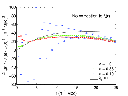
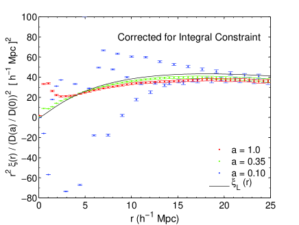
Our reproduction of the $P$-sampled $\Lambda$CDM simulations presented in Fig. 9 of Sirko 2005 [2], shown here in the left panel of Fig. 1, indicates that this measurement bias is quite important for the $L_{\rm box}=100\,h^{-1}$Mpc simulations they present, suppressing the correlation function at 1/4th the scale of the box by almost a factor of two and causing a severe disagreement with the linear theory correlation function for $r\sim 20-25\,h^{-1}$Mpc despite the fact that $\xi_{L}(r)\ll 1$ on these scales.

To correct for this measurement bias, following the approach used in Orban & Weinberg [33], one defines

$$\xi_{{\rm uni},i}(r)=\xi_{{\rm uni,true},i}(r)+\xi_{\rm bias}$$ (3.22)

where $\xi_{\rm bias}$ is a radially-independent term and $\xi_{{\rm uni,true},i}(r)$ is understood to be the correlation function of the box without the integral-constraint bias. Using Eq. 3.21, $\xi_{\rm bias}$ can be solved for, giving

$$\xi_{\rm bias}=-\frac{3}{R_{\rm box}^{3}}\int_{0}^{R_{\rm box}=L_{\rm box}/1.61}\xi_{{\rm uni,true},i}(r)\,r^{2}dr\approx-\frac{3}{R_{\rm box}^{3}}\int_{0}^{R_{\rm box}=L_{\rm box}/1.61}\xi_{L}(r)\,r^{2}dr$$ (3.23)

where the integral over $\xi_{{\rm uni,true},i}(r)$, which is weighted heavily towards large scales, has been well approximated using linear theory. The corrected estimator for the correlation function is therefore

$$\xi_{{\rm uni,true},i}(r)=\xi_{{\rm uni},i}(r)-\xi_{\rm bias}=\xi_{{\rm uni},i}(r)+\frac{3}{R_{\rm box}^{3}}\int_{0}^{R_{\rm box}=L_{\rm box}/1.61}\xi_{L}(r)\,r^{2}dr.$$ (3.24)

This result is identical to the prescription presented in Orban & Weinberg [33]. Results from using the integral-constraint corrected estimator are presented in the right panel of Fig. 1. For separations of $r\sim 20-25h^{-1}$ Mpc the amplitude of the correlation function is nearly a factor of two higher at all epochs, which agrees much better with the linear theory correlation function on these scales as would be expected. Therefore the conclusion in Sirko 2005 that $P$-sampled simulations suppress the correlation function for separations approaching the box scale is found to stem from an overlooked integral-constraint correction. Importantly, as is clear from Fig. 1, the integral constraint correction matters for separations as small as $r\sim 10\,h^{-1}$ Mpc $\sim L_{\rm box}/10$ or perhaps slightly smaller. While most practitioners would regard clustering measurements at separations of $r\sim L_{\rm box}/4$ or $r\sim L_{\rm box}/5$ in a simulation volume to be too large compared to the scale of the box to be trustworthy, it should be received with some amount of surprise that clustering measurements at separations as small as $r\sim L_{\rm box}/10$ are significantly biased, independently-of-epoch in conventional, $P$-sampled simulations. Thankfully, correlation function measurements at these scales can be corrected using Eq. 3.24 without re-running the simulation and Appendix A provides a useful independent-of-epoch formula for $\Lambda$CDM simulations that can estimate this bias at the BAO scale given the size of the simulation box.

3.4 Integral-Constraint Bias in $\xi$-sampled Simulations

Returning to the conclusions of Sirko [2] one may ask why the $\xi$-sampled results in [2] agreed so well with linear theory approaching the box scale if Sirko did not also apply an integral constraint correction to the $\xi$-sampled correlation function measurements? The answer is that Eq. 3.8 (which is what Sirko used) includes, in its average, a term very much like the integral constraint correction. At large enough separations in the simulation box, the particle distribution will be approximately uncorrelated ($\xi_{{\rm box},i}(r)\approx 0)$. On these scales Eq. 3.8 gives

$$\xi_{{\rm uni},i}(r)\approx\left(\frac{a_{\rm uni}}{a_{{\rm box},i}}\right)^{6}-2\left(\frac{a_{\rm uni}}{a_{{\rm box},i}}\right)^{3}+1=\left(1+\Delta_{i}\right)^{2}-2\left(1+\Delta_{i}\right)+1=\Delta_{i}^{2}$$ (3.25)

with $\Delta_{i}\equiv\frac{D(a_{\rm uni})}{D(1)}\Delta_{0,i}$ as used elsewhere. Taking the average over many realizations $i$,

$$\langle\xi_{{\rm uni},i}(r)\rangle=\langle\Delta_{i}^{2}\rangle=\frac{P_{\rm real}(0)}{L_{\rm box}^{3}}\frac{D^{2}(a_{\rm uni})}{D^{2}(1)}=\frac{4\pi}{L_{\rm box}^{3}}\int_{0}^{L_{\rm box}/2}\xi_{L}(r)\,r^{2}{dr}$$ (3.26)

While not exact, the term $P_{\rm real}(0)/L_{\rm box}^{3}$ is very similar to the $\xi_{\rm bias}$ correction term in Eq. 3.23 & 3.24. It is this term that does the work, so to speak, of correcting for the integral constraint in the $\xi$-sampled simulations in [2]. This is why Sirko concluded that the $\xi$-sampled method matched well with linear theory on scales approaching the box without an explicit correction term. If this $\Delta_{i}^{2}$ term had not emerged (as it does in Eq. 3.25, essentially by accident) the $\xi$-sampled correlation function results would have been suppressed much like the $P$-sampled result shown in the left panel of Fig. 1. But since the term does appear there is no need to explicitly correct for the integral constraint bias in $\xi$-sampled simulations. Instead the correction is understood to be built into Eq. 3.8, which is the formula employed in all the $\xi$-sampled correlation function measurements presented here.

4 $\xi$-sampled ICs with Powerlaw Models

For powerlaw models, where $P(k)=Aa^{2}k^{n}$, the task of computing Eq. 2.2 is made substantially easier because an exact analytic solution for $\xi_{L}(r)$ is known in this case,

$$\xi_{L}(r)=\left(\frac{r_{0}}{r}\right)^{n+3},\,A\,a^{2}=\frac{2\pi^{2}\,r_{0}^{n+3}\,\,(2+n)}{\Gamma(3+n)\sin((2+n)\pi/2)}~{},$$ (4.1)

[41]. Eq. 2.2 therefore becomes

$$P_{\rm{real}}(k)=4\pi r_{0}^{n+3}\int_{0}^{L_{\rm box}/2}r^{-(n+1)}\,\frac{\sin kr}{kr}\,{dr}.$$ (4.2)

Eq. 4.2 can be used straightforwardly to express the DC power,

$$\displaystyle P_{\rm{real}}(0)\,= \displaystyle 4\pi r_{0}^{n+3}\int_{0}^{L_{\rm box}/2}r^{-(n+1)}\,{dr}$$ (4.3)

$$= \displaystyle\frac{2^{n+2}\pi}{-n}\left(\frac{r_{0}}{L_{\rm box}}\right)^{n+3}L_{\rm box}^{3}.$$ (4.4)

Analytic and special-function solutions to Eq. 4.2 exist for certain powerlaws. In this study I am interested in $n=-1$, $-1.5$ and $-2$ which can be expressed by

$$P_{\rm{real},n=-1}(k)= 4\pi r_{0}^{2}\,\rm{Si}(kL_{\rm box}/2)\,k^{-1},$$ (4.5)

$$P_{\rm{real},n=-1.5}(k)= 2^{5/2}\pi^{3/2}r_{0}^{3/2}\,\rm{S}(\sqrt{kL_{\rm box}}/\sqrt{\pi})k^{-1.5},$$ (4.6)

$$P_{\rm{real},n=-2}(k)= 8\pi r_{0}\,\sin^{2}(kL_{\rm box}/4)\,k^{-2},$$ (4.7)

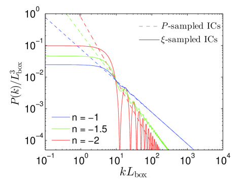
where $\rm{Si}(x)$ is the sine integral and S($x$) is a Fresnel integral. These formulae can be very useful for generating accurate initial conditions, especially for steep power spectra. I show these power spectra in Fig. 2, fixing $r_{0}/L_{\rm box}=1/16$ to set the relative amplitudes. Notice that steeper powerlaws have larger DC power, easily seen on the plot as the asymptotic value of $P_{\rm{real}}(k)/L_{\rm{box}}^{3}$ as $k\rightarrow 0$. Noticing that $P(k)$ does not go to zero at small $k$ for the $P$-sampled powerlaws, one might be concerned that these models are unphysical. However, despite the high levels of large scale clustering power the rms overdensity in spheres and other statistics can remain finite for $n>-3$. It so happens that a close inspection of Eq. 4.2 reveals that $P_{\rm real}(k)$ is finite and positive (or equal to zero) for all $k$ only if $n\geq-2$. It is unclear how to circumvent this issue to simulate steeper power spectra. For $\Lambda$CDM initial conditions this limitation translates into assuming $L_{\rm box}\gtrsim\,2.5h^{-1}$ Mpc to avoid $P_{\rm real}(k)<0$ because the effective slope of the $\Lambda$CDM correlation function at small scales, using $\xi_{L}(r)=(r_{0}/r)^{n_{\rm eff}(r)+3}$, is $n_{\rm eff}\lesssim-2$ for $r\lesssim 2.5\,h^{-1}$ Mpc.

Figure 2: A comparison of $P$-sampled and $\xi$-sampled pure powerlaw models. $\xi$-sampled power spectra are computed from Eq. 2.2 and used to generate initial conditions for that method. $r_{0}/L_{\rm{box}}=1/16$ is chosen to set the overall amplitude of each model. To compare with $\xi$-sampled spectra for $\Lambda$CDM initial conditions see Fig. 2 of [2].

4.1 Scale free?

Although pure powerlaw models are often referred to in the literature as “scale free,” since $P(k)=Ak^{n}$ is featureless, the $\xi$-sampled initial power spectra shown in Fig. 2 clearly depend on the choice of $L_{\rm box}$. In practice, these oscillatory features die away in simulations and the effect of the box size is merely to change the variance of the DC mode (which is set by $P_{\rm{real}}(0)/L_{\rm box}^{3}$).

Since dark energy introduces a new scale into the problem (e.g. the age of the universe when $\rho_{m}=\rho_{\Lambda}$), I consider only $\Omega_{m,\rm{uni}}=1.0,\Omega_{\Lambda,\rm{uni}}=0,\Omega_{k,\rm{uni}}=0$ so as to keep the simulations as “scale free” as possible and allow the self-similar tests discussed in the next section. In the Zeldovich [21] and adhesion [42, 43] approximations (as in linear theory), the effect of dark energy on structure formation is entirely captured by changing the linear theory growth function. [44] and [45] convincingly argue that this approximation is remarkably accurate even in the non-linear regime – the second order effect of dark energy is relatively small. Therefore the results of my $\Omega_{m}=1$ tests should still be quite relevant to studies that include a dark energy component.

As one final comment on the scale-free nature of my simulations, throughout I adopt, as a time variable,

$$\frac{a}{a_{*}}=\left(\frac{k_{\rm{box}}}{k_{\rm{NL}}}\right)^{(n+3)/2}~{},$$ (4.8)

where $k_{\rm{box}}\equiv 2\pi/L_{\rm{box}}$ and $k_{\rm{NL}}$ is defined by the dimensionless linear theory power spectrum, $\Delta_{L}^{2}(k_{\rm{NL}})\equiv 1$. The scale-free nature of the simulations demands that only the ratio $a/a_{*}$ is meaningful (e.g. as the square root of the dimensionless power on the scale of the box) and so $a_{*}$ is defined implicitly in the definitions already given. Eq. 4.8 is also simply related to the $\sigma_{\rm{miss}}$ formula of [46], which quantifies the missing power on the scale of the box in $P$-sampled simulations as another choice for a time variable. I adopt Eq. 4.8 for ease of comparison with [47] and because the $\sigma_{\rm{miss}}$ formula in [46] would be inappropriately applied to $\xi$-sampled simulations, which have a turnoff in $P_{\rm real}(k)$ near the box scale (Fig. 2).

Figure 3: Measured matter autocorrelation functions from conventional $P$-sampled (left panels) and $\xi$-sampled (right panels) ensembles of simulations. The upper two panels show results from an initially $n=-1$ power spectrum, middle panels show results from $n=-1.5$, and the lower two panels show $n=-2$. In each plot the $x$-axis is scaled by the non-linear scale, $r_{0}$, where $\xi_{L}(r_{0})\equiv 1$ so that, if evolving with the expected self-similar behavior, the outputs should lie upon the same locus of points. The $y$-axis is scaled by $\xi_{L}(r)=(r_{0}/r)^{n+3}$. Black lines show fitting functions for the self-similar correlation function from high resolution ($P$-sampled) simulations for comparison. Error bars show measured error on the mean. Note that the first outputs in each plot are affected by transients from initial conditions.

5 $\xi(r)$ results

5.1 Powerlaw Models

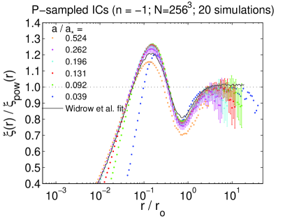
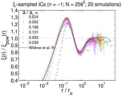
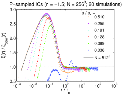
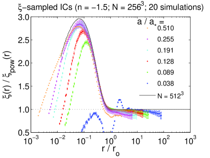
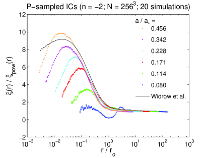
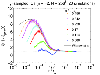
Fig. 3 shows my primary results for the self-similar scaling of the matter correlation function. The x-axis is shown in $r/r_{0}$ units where $\xi_{L}(r_{0})\equiv 1$. Insofar as the dark matter clustering is negligibly affected by numerical limitations such as the finite scale of the box or the scale of the force softening, with this scaling the correlation function results from different outputs should all lie upon the same line. To the extent that this is achieved the correlation function can be said to evolve with self-similarity and it is clear from Fig. 3, excluding the first outputs which are severely affected by transients from initial conditions, that over a wide range of scales the results from these relatively modest, $N=256^{3}$, simulations do fall upon the the same locus as expected. This locus is different for each powerlaw; for steeper power spectra (e.g. $n=-2$) power is transferred from large scales to small scales and the non-linear growth of $\xi(r)$ out paces linear theory whereas for shallower power spectra (e.g. $n\gtrsim-1$) there is so much small scale power that the process of halo formation and collapse causes the non-linear growth to fall behind linear theory in a process sometimes called “pre-virialization” [39]. In the language of the halo model [48] this implies that the predicted linear theory clustering on small scales is so high that the amplitude of the 1-halo term is below the linear theory clustering amplitude on those scales. The $n=-1$ case falls between these two extremes and the amplitude of the correlation function is both above and below linear theory, depending on the regime. (For a bracketing case of an even shallower power spectrum see, e.g., the $n=-0.5$ results in [33, Appendix A].)

In Fig. 3, the $\xi$-sampled and $P$-sampled methods generally agree well on the shape of the self-similar solution. This is significant for the $\xi$-sampled results, on some level verifying the method. Alongside the measurements in each case fitting functions for the self-similar correlation function from higher resolution simulations are shown (black lines). For $n=-1$ and $n=-2$ this comparison is made by numerically fourier transforming the non-linear power spectrum fitting functions published in [47]; note in the $n=-1$ case I include subtle but important corrections to their fit at small $k/k_{\rm{nl}}$ as determined in [33, Appendix A]. For $n=-1.5$, I compare with $\xi(r)$ measurements from 10 $P$-sampled simulations with $N=512^{3}$ [33, Appendix A]. These high-resolution results are used more quantitatively in Fig. 4 where the correlation function results are presented relative to the box size. Overall, the agreement with the high-resolution self-similar results is quite good and excluding the initial and final outputs in each case my simulation set tends to match the self-similar evolution to better than about 5% in most outputs and on most scales. This is similar to the precision on the results from higher-resolution simulations. The last output is excluded from this conclusion since the linear theory clustering level is so high that one expects departures from the true non-linear clustering from the suppression of power on the scale of the box. Also, the correction for the integral constraint, which assumes a linear theory correlation function in $\xi_{\rm bias}$ (Eq. 3.23), likely becomes inaccurate in the highly-clustered regime as well.

Another caveat to the overall good agreement is at small $r/r_{o}$ especially for early outputs. Fig. 4 presents the same correlation function measurements in Fig. 3 relative to the scale of the simulation box and shows that these deviations from self-similarity are all below the scale of the initial mean interparticle spacing. This is as expected since at best the initial conditions will only match the self-similar solution down to these separations. Rather than excluding these scales from Fig. 3, they are included to highlight, in Fig. 4, that as structure evolves the self-similar behavior extends further and further below this scale, in some cases approaching the force softening. This result is non-trivial and difficult to anticipate from first principles.

Figure 4: Measured correlation functions from simulations (colored points) relative to high-resolution results for the self-similar scaling ($\xi_{ss}(r)$; black lines in Fig. 3). Panels are organized as in Fig. 3 (left panels: $P$-sampled results, right panels: $\xi$-sampled results, $n=-1,-1.5$ and $-2$ from top to bottom). Vertical lines show relevant numerical scales: the initial mean interparticle spacing (dotted black), the Particle-Mesh Grid Scale (dot-dashed black), and the force softening (dashed black).

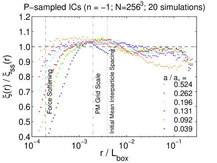
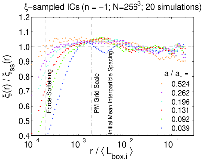
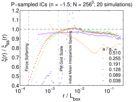
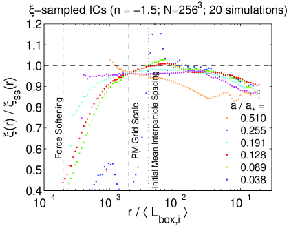
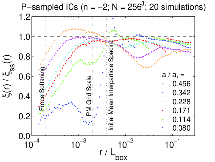
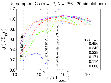
It bears mentioning some of the previous work on how non-linear clustering proceeds near or below the scale of the initial mean interparticle spacing. [49], using $n=-1$ simulations, show that Fourier modes in the non-linear regime are largely determined by the collapse of large-scale modes rather than by evolution of power initially on those scales. This nicely explains the trend in Fig. 4 for later outputs to match better with the self-similar solution on small scales and why the poisson noise in the dark matter density on those small scales does not prevent this from happening. However, Joyce et al. [50] and collaborators have argued that the common practice of setting the force softening significantly smaller than the initial mean interparticle spacing (as in the simulations presented here) introduces errors which arise from the possibility that with this choice the equations of motion for the particles are no longer true to the Vlasov-Poisson fluid equations. Despite this, their results concur with Fig. 4 that $\xi(r)$ can reliably be modeled below the scale of the mean interparticle spacing. According to [50] the main effect of aggressive force softening is to cause $\sim 5\%$ disagreement with the true non-linear $\xi(r)$ on scales larger than the mean interparticle spacing. The $P$-sampled results shown in Fig. 4 are in qualitative agreement with the simulations presented in [50] in the sense that accurate non-linear behavior is observed below the mean interparticle spacing and on larger scales the measurements are consistent with the self-similar solution also at the level of $\sim 5\%$. Although beyond the scope of this paper, it would be interesting to run the $P$-sampled simulation set with less aggressive force softening (e.g. half the mean interparticle spacing) to test if the measured error on the mean $\xi(r)$ is detectably smaller, as predicted in [50]. At any rate, for all three powerlaws the self-similar behavior extends well below the scale of the mean interparticle spacing; it does not significantly depend on whether power is being rapidly “transferred” to smaller scales as for $n=-1.5$ and $n=-2$ or whether the non-linear growth proceeds less quickly than the linear theory prediction on small scales (i.e. $r<r_{0}$), as for $n=-1$.

5.2 Powerlaw Times a Bump Results

Figure 5: Correlation function results from ensembles of 20 $\xi$-sampled simulations using initial conditions consistent with a powerlaw times a gaussian bump as a simplified model of baryon acoustic oscillations. Dot-dashed lines show results from the high-resolution simulations presented in [33, Fig. 3]. Typical errors on the mean for the $\xi$-sampled results are shown offset to the right. The initial bump width and height from the initial conditions is shown with a dashed black line. Note that in the $n=-0.5$ panel in the top left, for ease of comparison the dot-dashed lines are derived from gaussian fits to the $P$-sampled results instead of simply presenting the actual correlation function measurement as in the other panels because these measurements are somewhat noisy.

Figure 6: Results from gaussian fits to the simulation results presented in Fig. 5. Each plot shows best-fit quantities versus $r_{o}/r_{\rm bao}$ (i.e. the time variable) for all three powerlaws, cyan for $n=-0.5$, green for $n=-1$ and red for $n=-1.5$. Upper left: the best-fit position of the peak. Upper right: the best fit amplitude of the BAO feature. Bottom left: gaussian width of the BAO feature. Bottom right: the normalized area of the BAO feature. Errorbars throughout are derived from jackknife error estimation.

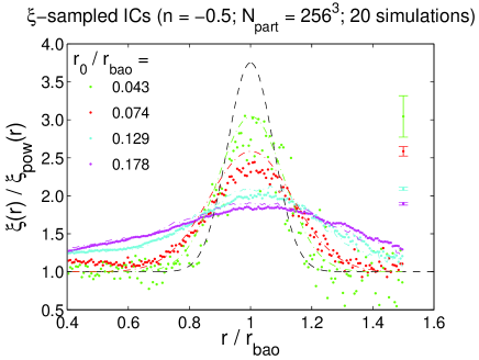
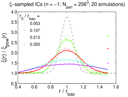
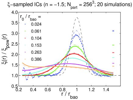
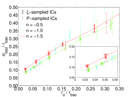
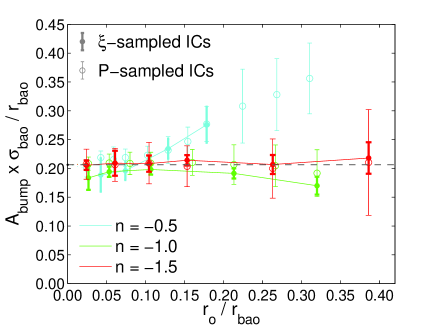
As discussed in depth in [33], a real-space powerlaw times a bump can be used as a self-similar numerical test in addition to providing insight into the non-linear physics of the evolution of the BAO feature. In this case,

$$\xi_{L}(r)=\left(\frac{r_{0}}{r}\right)^{n+3}(1+A_{\rm{bump}}\,e^{-(r-r_{\rm{bao}})^{2}/2\sigma_{\rm{bao}}^{2}}),$$ (5.1)

and for resemblance to the $\Lambda$CDM correlation function I chose $A_{\rm{bump}}=2.75$, $\sigma_{\rm{bao}}/r_{\rm{bao}}=0.075$, and powerlaws of $n=-0.5$, $-1$, and $-1.5$. Unlike $\Lambda$CDM, this setup can be evolved much further than $\sigma_{8}\sim 1$ to investigate the non-linear physics of the problem. For each powerlaw, in Fig. 5 I compare results from 20 $\xi$-sampled simulations with $N=256^{3}$, $r_{\rm{bao}}/\langle L_{{\rm box},i}\rangle=1/20$ to the results of 7 $P$-sampled, $N=512^{3}$, $r_{\rm{bao}}/L_{\rm{box}}=1/20$ simulations from [33]. In Fig. 5 these $P$-sampled results are shown with dot-dashed lines of various colors corresponding to different outputs. Since the first two outputs from the $P$-sampled $n=-0.5$ simulations are noisy because of the very low clustering amplitude, Fig. 5 presents the best fit gaussians to those results for ease of comparison. All other dot-dashed lines are the mean correlation function results from the $P$-sampled simulations. Error bars in Fig. 5 show the error on the mean for the $\xi$-sampled results. Qualitatively, the correlation function results agree well and importantly the non-linear shift in the $n=-1.5$ results and lack of shift in the $n=-0.5$ and $-1$ results are consistent. This conclusion should be reassuring to the wider effort to characterize the non-linear shift of the BAO peak using standard $P$-sampled simulations.

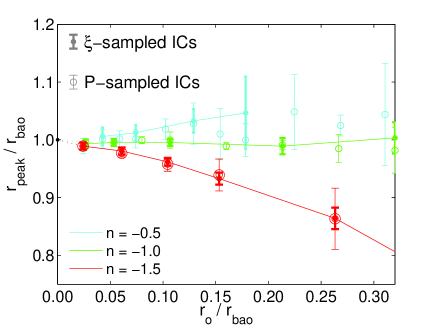
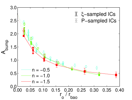
A quantitative comparison of the results in Fig. 5 is presented in Fig. 6. Here the $\xi$-sampled results are shown with solid points with thick error bars, and the $P$-sampled results are shown as open circles with thin error bars, both with colors corresponding to the powerlaw (cyan for $n=-0.5$, green for $n=-1$, and red for $n=-1.5$). As in Fig. 5 of Orban & Weinberg [33], the error bars for both methods come from jackknife error estimation by sequentially omitting one of the realizations and computing the best fit gaussian and shift of the peak. The $\xi$-sampled results typically have tighter error bars than the $P$-sampled results because more $\xi$-sampled simulations were performed.

The upper left panel of Fig. 6 echoes what was said earlier that the non-linear shift of the BAO peak is consistent between the two methods. The $n=-0.5$ results for both methods show some preference for a BAO shift to slightly larger scales, however the shift in this case is degenerate with the broadening (notice that the error bars in the bottom left plot are relatively large at later outputs) and the error bars are consistent with no movement of the BAO peak. A real movement of the peak to larger scales would have been counter-intuitive since the non-linear physics of the shift stems from a small but non-negligible tendency for particle pairs with initial separations of $r=r_{\rm bao}$ to be found in regions with a slight overdensity, causing (on average) a very small movement inward [53].

Fortunately for BAO surveys, the broadening of the BAO feature from the growth of structure is a much larger effect than the non-linear shift. The bottom left panel of Fig. 6 highlights the results for broadening of the gaussian width of the BAO feature as it evolves from its initial value of $\sigma_{\rm bao}/r_{\rm bao}=0.075$. The results from the two methods compare well and there are no pairs of points from any particular output or powerlaw that are statistically inconsistent with each other. In Fig. 5 of Orban & Weinberg [33] a very similar plot compared these $P$-sampled results to a simple diffusion model inspired by [53]. This earlier comparison was reasonably good and remarkably the $n=-1.5$ results agreed with an ab initio prediction of the diffusion model. The agreement between the $\xi$-sampled and $P$-sampled results argues that this same physics is properly included in $\xi$-sampled simulations and, e.g., that including the DC mode fluctuations in overdensity does little to change this result.

The top right panel of Fig. 6 presents the results for the amplitude of the BAO feature. At later outputs the two methods agree well, however there is some tension with the first few outputs. This would be concerning except that the $P$-sampled $N=256^{3}$ results in Fig. 8 of Orban & Weinberg [33] show a similar decrement in bump amplitude compared to $N=512^{3}$ $P$-sampled simulations at early outputs. This mismatch seems to be some finite-particle numerical effect as opposed to some orthogonal concern relating to box scale cutoffs of large scale power. The bottom right panel shows the results for the normalized area of the bump, $A_{\rm bump}\times\sigma_{\rm bao}/r_{\rm bao}$ which tends to be constant in spite of the non-linear evolution of the BAO feature in agreement with the diffusion model discussed in Orban & Weinberg [33]. In the $\xi$-sampled simulations at early outputs the bump area falls somewhat below its initial value for both $n=-0.5$ and $-1$ by about one sigma. This can be attributed to the decrement of $A_{\rm bump}$ since $\sigma_{\rm bao}$ evolves as expected, but more importantly this tension with the constant-bump-area evolution at these early outputs seems to corroborate the conclusion that it is merely an inaccuracy from using $N=256^{3}$ particles instead of $N=512^{3}$.

6 Box-to-Box Variance of the Correlation Function

6.1 Preliminaries

Having explored the ensemble-averaged predictions for the mean $\xi(r)$, in this section I compare the results for the box-to-box variance of $\xi(r)$ from the $\xi$-sampled and $P$-sampled methods, focusing on separations approaching the box scale ($r\gtrsim L_{\rm box}/10$). While the variance (or, more generally, covariance) of statistics like $\xi(r)$ is important for surveys so as to precisely and accurately infer cosmological constraints from a finite data set [9, 52, 54, 55, 56, 10], the primary goal of this section is somewhat more prosaic. Namely, if the box-to-box variance of $\xi(r)$ from one or the other method is substantially larger then substantially more simulations must be performed via this method to obtain the same precision on the mean $\xi(r)$. This would be the only reason to perform additional simulations since § 3.3 and § 5 show that as long as the integral constraint correction is applied to $P$-sampled correlation function measurements, the mean $\xi(r)$ is consistent between the two methods.

The box-to-box variance comes from the (usual) definition,

$${\rm Var}(\xi)=\langle(\xi_{{\rm uni},i}(r)-\xi(r))^{2}\rangle=\frac{1}{N_{\rm sims}-1}\sum_{i=1}^{N_{\rm sims}}\,\left(\xi_{{\rm uni},i}(r)-\xi(r)\right)^{2}$$ (6.1)

where $\xi_{{\rm uni},i}(r)$ is a correlation function measurement from an individual box. For $\xi$-sampled simulations, since the overdensity of each box is perturbed from the mean density of the true cosmology, one must use Eq. 3.8 to “convert” $\xi_{{\rm box},i}(r)$ (a statistic that assumes incorrectly that the overdensity of the box is zero) to $\xi_{{\rm uni},i}(r)$ as discussed in § 3. For $P$-sampled simulations this step is unnecessary because every realization has zero overdensity by design and consequently $\xi_{{\rm uni},i}(r)=\xi_{{\rm box},i}(r)$.

This section will discuss three different sources of box-to-box variance (or, equivalently, three different considerations that degrade the precision on the mean $\xi(r)$ from a finite number of simulations). These sources are: (1) variance from ignorance of the overdensity of the realizations, (2) variance from measuring $\xi(r)$ from a finite number of randomly realized density fields, and (3) variance from correlations on weakly to strongly non-linear scales.

The first item is mentioned only for completeness. As discussed in § 3, the $\xi$-sampled correlation function estimator in Eq. 3.8 is implicitly “informed” of the overdensity and likewise the $P$-sampled estimator is informed of the overdensity in the sense that the overdensity of each box is identically zero. Were this not the case, then on large scales where the correlation is weak, following the discussion in § 3.2 the correlation function measurement would yield the overdensity of the box at that epoch, $\xi_{{\rm uni},i}(r)\approx 2\Delta_{i}$, and applying Eq. 6.1 one would find

$${\rm Var}(\xi)\approx\langle(2\Delta_{i}-0)^{2}\rangle=4\,\langle\Delta_{i}^{2}\rangle=4\,\frac{P_{\rm real}(0)}{L_{\rm box}^{3}}\frac{D^{2}(a_{\rm uni})}{D^{2}(1)}.$$ (6.2)

In the powerlaw models investigated in this section but certainly also in $\Lambda$CDM cosmologies the above result would be an order of magnitude larger than any of the other sources of box-to-box variance just mentioned and many more simulations would need to be performed to measure the mean $\xi(r)$ with any kind of precision. This underscores the importance of using a “better informed” estimator for which $\xi_{{\rm uni},i}(r)=0$ when the particles are uncorrelated. The cost of using an estimator that is ignorant of the overdensity is severe.

One may ask, then, what Eq. 6.1 really means for $\xi$-sampled simulations using a “better informed” estimator. The answer is that the definition of the variance is not substantially changed. Eq. 6.1 is the variance (or, equivalently, width of the distribution) of correlation function measurements at a particular separation, $r$, from finite volumes in a situation where the mean density of the universe is perfectly known and the overdensities of each volume are also perfectly known. In other words, the only unknown is $\xi(r)$, which is what we are trying to measure. This is exactly as it would be in a $P$-sampled ensemble of simulations where all overdensities are perfectly known to be zero and the mean density of the universe is likewise perfectly known. So although the task of measuring $\xi(r)$ is somewhat more complicated in $\xi$-sampled simulations (i.e. because of Eq. 3.8 and the volumetric weighting), the measurement in principle is not qualitatively different from $P$-sampled ensembles. This being the case, the most important source of variance for both methods comes from the fact that we are trying to measure the mean correlation function of the universe from a finite number of randomly-realized density fields with known overdensities.

6.2 Expectations from Gaussian Statistics

Mindful that the correlation function is also the fourier transform of the power spectrum (Eq. 2.1), the statement just made regarding the most important source of variance can also be conveyed by pointing out that finite volumes contain a finite number of fourier modes that can be used to compute statistics like the correlation function. Since the number of modes in the simulation box for each $k$ value is straightforwardly determined this consideration can be used to estimate the variance of $\xi(r)$ using a linear theory approximation for $P(k)$. Applying this reasoning one arrives at an estimate for the variance,

$$\sigma_{\xi}^{2}=\frac{1}{V\pi^{2}}\int_{0}^{\infty}{dk}k^{2}\left(\frac{\sin kr}{kr}\right)^{2}P(k)^{2}$$ (6.3)

[55]. This is referred to as a “gaussian” estimate of the variance because in the approximation of gaussian random fields, wherein all higher order statistics (e.g. 3-point and 4-point functions) are assumed to be negligible, Eq. 6.3 perfectly models the variance of $\xi(r)$. For pure powerlaw models, $P(k)=Ak^{n}$, it can be shown using Eq. 6.3 that

$$\frac{\sigma_{\xi}}{\xi_{\rm{pow}}(r)}=\frac{A_{n}}{\pi}\frac{\sqrt{\Gamma(1+2n)\sin n\pi}}{4^{(n+1)/2}}\left(\frac{r}{L_{\rm{box}}}\right)^{3/2}$$ (6.4)

where $A\equiv A_{n}r_{0}^{n+3}$, and $\Gamma(1+2n)$ is the usual gamma function. Notice that all of the $r_{0}$ dependence has canceled out with the division by $\xi_{\rm{pow}}(r)=(r_{0}/r)^{n+3}$. Unfortunately, Eq. 6.4 is only convergent for the limited range of $-1.5<n<-0.5$.

Figure 7: Measurements of the box-to-box variance of $\xi(r)$ from simulations (colored points in each panel, see Fig. 3 for legends) compared to expectations from gaussian statistics (Eq. 6.3 in dashed black lines, and Eq. 6.3 with a low-$k$ cutoff for the integral at $k_{\rm box}=2\pi/L_{\rm box}$ shown with solid gray lines). The $x$-axis shows the separation, $r$, relative to the scale of the simulation box. Also shown alongside measurements from $\xi$-sampled simulations is an extra source of variance from Eq. 6.6. Note that the $\xi$-sampled measurements do not extend to separations as close to the box scale as the $P$-sampled measurements. In highly overdense boxes, this avoids measuring $\xi(r)$ for separations larger than $L_{{\rm box},i}/4$.

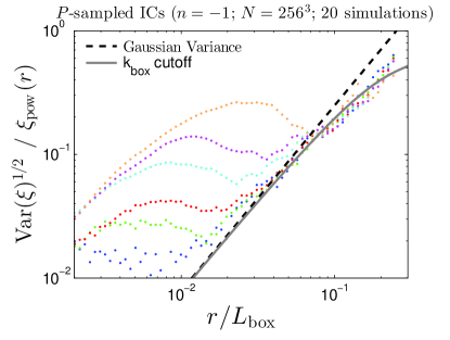
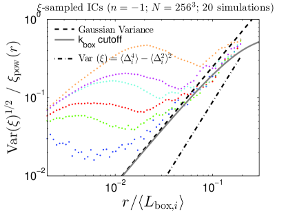
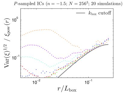
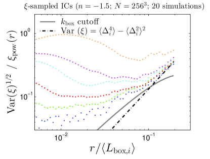
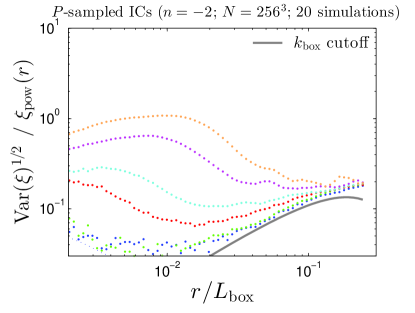
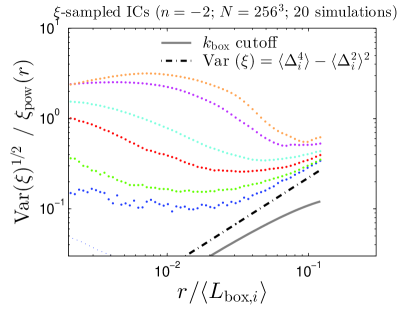
Fig. 7 compares Eq. 6.3 with a low-$k$ cutoff at $k_{\rm box}$ (solid gray lines) to the box-to-box variance measured from the simulation ensembles in detail, showing the separation, $r$, relative to the scale of the box and normalizing the $y$-axis by $\xi_{\rm pow}(r)$ so that the gaussian expectation of Eq. 6.4 is independent of epoch. For the convergent case of $n=-1$, Eq. 6.4 without a low-$k$ cutoff (dashed black lines) is also compared to the simulation data. The $\xi$-sampled results are also compared to another source of variance (black dot-dashed lines, Eq. 6.6) that will be explained in the next section.

6.3 Commentary on Figure 7

The $n=-1$ results in Fig. 7 are most instructive since Eq. 6.3 is compared to the measured variance from simulations both with and without the low-$k$ cutoff. In each panel in Fig. 7 the range $r/L_{\rm box}\gtrsim 1/10$ is most important for this comparison because on smaller scales and increasingly for later outputs the box-to-box variance from non-linear correlations, which are not accounted for in Eq. 6.3, become important and greatly exceed the linear theory expectation of Eq. 6.3. But for $r/L_{\rm box}\gtrsim 1/10$, the $n=-1$ case measurements of the variance generically fall below Eq. 6.3 without the low-$k$ cutoff and are either consistent with or slightly above the expected variance from including the low-$k$ cutoff in Eq. 6.3. That both methods fall below the expectation of Eq. 6.3 without the low-$k$ cutoff is a sensible result, especially for $P$-sampled simulations because it is an explicit assumption of the method that $P(k)=0$ for all $k$-modes from scales larger than the size of the simulation box. As a result, clustering power on these scales do not contribute to the box-to-box variance of $\xi(r)$.

The $\xi$-sampled $n=-1$ results falling below the expectation of Eq. 6.3 is also sensible for two reasons: (1) as argued earlier, the definition of the box-to-box variance is not substantially changed. And (2) despite including the fluctuations in the DC mode of the simulations, one still expects the $\xi$-sampled method to under-represent clustering on scales larger than the box. Notice, for example, that $P_{\rm real}(k)$ is totally insensitive to clustering power in $\xi(r)$ from $r>L_{\rm box}/2$ (Eq. 2.2) and it is $P_{\rm real}(k)$ that is used in the Zel’dovich formulism to generate the initial conditions.

Turning to the $n=-1.5$ and $-2$ results, clearly the measurements from the $P$-sampled simulations for $n=-1.5$ and $-2$ also compare well to the expectation from Eq. 6.3 with a cutoff at $k_{\rm box}$ as expected. However, the $\xi$-sampled results clearly exceed the expectation of Eq. 6.3 with the low-$k$ cutoff. This stems from the fact that, compared to the $n=-1$ simulations, the fluctuations in the overdensity are larger for the $n=-1.5$ simulations and even larger for the $n=-2$ simulations (c.f. $P_{\rm real}(k\rightarrow 0)$ in Fig. 2). But the key is that in $\xi$-sampled simulations the correction for the integral constraint bias arises naturally because $\xi_{{\rm uni},i}(r)~{}\rightarrow~{}\Delta_{i}^{2}$ on large scales where the particle distribution is approximately uncorrelated (Eq. 3.25). When this is the case, the box-to-box variance (Eq. 6.1) yields

$${\rm Var}(\xi)\approx\langle(\Delta_{i}^{2}-\langle\Delta_{i}^{2}\rangle)^{2}\rangle=\langle\Delta_{i}^{4}\rangle-\langle\Delta_{i}^{2}\rangle^{2}.$$ (6.6)

Since $\Delta_{i}=\frac{D(a_{\rm uni})}{D(1)}\Delta_{0,i}$ and $\Delta_{0,i}$ is a gaussian random variable, then $\langle\Delta_{i}^{4}\rangle=3\langle\Delta_{i}^{2}\rangle^{2}$ and

$${\rm Var}(\xi)=3\langle\Delta_{i}^{2}\rangle^{2}-\langle\Delta_{i}^{2}\rangle^{2}=2\,\langle\Delta_{i}^{2}\rangle^{2}=2\,\left(\frac{P_{\rm real}(0)}{L_{\rm box}^{3}}\frac{D^{2}(a_{\rm uni})}{D^{2}(1)}\right)^{2}.$$ (6.7)

Although the above expression is smaller than, e.g., Eq. 6.2 it can be as large or larger than Eq. 6.3. So while the expectation of Eq. 6.3 with a low-$k$ cutoff compared well to the measurements from simulation in all the other panels, this is why the $\xi$-sampled $n=-1.5$ and $-2$ results in Fig. 7 so greatly exceed the expectation from Eq. 6.3 with the low-$k$ cutoff even in the $r\gtrsim L_{\rm box}/10$ region where non-linear effects are small.

In $\xi$-sampled $\Lambda$CDM simulations, such as those in Sirko [2], this issue would likewise artificially increase the box-to-box variance and degrade the error on the mean $\xi(r)$. If the box size is small enough then $\langle\Delta_{i}^{4}\rangle^{1/2}$ will be comparable to $\sigma_{\xi}$ from Eq. 6.3 . Indeed this seems to be the case in their Fig. 9 which presents $\xi$-sampled simulations with $L_{\rm box}=100~{}h^{-1}$ Mpc. The 1-sigma error on the mean $\xi(r)$ in that case is noticeably larger than the 1-sigma error on the mean from the $P$-sampled simulations. Sirko [2] does not comment on this interesting result. The work here suggests that this is just a consequence of $\xi_{{\rm uni},i}(r)\approx\Delta_{i}^{2}$ on the scale of the simulation box and how large typical values of $\Delta_{i}^{2}$ can be for 100 $h^{-1}$ Mpc boxes (c.f. their Fig. 4). Perhaps in future investigations a $\xi$-sampled estimator can be constructed to prevent this extra source of variance from contributing but without removing the compensation for the integral constraint bias (§ 3.4). Viewed another way, this additional complication with $\xi$-sampled simulations highlights the simplicity and economy of $P$-sampled simulations which with only a small correction for the integral constraint (Eq. 3.23) yields an unbiased estimate of the mean $\xi(r)$ and does so with a large-scale variance that corresponds very closely to the approximation of gaussian random fields as it should.

7 Summary and Conclusions

This paper explores the predictions from both the conventional method of running ensembles of cosmological simulations and an alternative approach proposed by [1] and implemented by [2]. The conventional method is dubbed the $P$-sampled approach because it aims to maximize the correspondence between the fourier space properties of the simulation and the fourier space statistics of the assumed cosmological model whereas [1] and [2] outline a $\xi$-sampled approach which is built from focusing on real-space statistics. Unlike the conventional method, the real-space approach allows the DC mode to vary from box to box. In an investigation comparing the $\xi$-sampled and $P$-sampled methods for the growth and evolution of the matter-matter two-point correlation function the following conclusions were drawn:

(1) Both $P$-sampled and $\xi$-sampled simulations give rise to the expected self-similar behavior from powerlaw initial conditions (specifically $n=-1,-1.5$ & $-2$). In the absence of exact solutions for the non-linear growth of structure these tests robustly evaluate the accuracy of the simulation method without assuming one or the other approach is correct [15].

(2) $\xi$-sampled simulations of BAO-inspired “powerlaw times a bump” models [33] yielded consistent results with earlier, higher-resolution $P$-sampled simulations for the broadening and shift of the BAO feature, even into the deeply non-linear regime ($\sigma_{8}\gtrsim 1$). A small but statistically significant discrepancy with the amplitude of the bump at early times can be attributed to a resolution effect.

(3) The earlier claim in Sirko 2005 [2] that the $\xi$-sampled method performs better than the $P$-sampled method in modeling the mean $\xi(r)$ in $\Lambda$CDM simulations for separations approaching the box scale is incorrect because of an overlooked integral-constraint correction to the $P$-sampled results presented there. Appendix A derives a simple, independent-of-epoch analytic formula for estimating the importance of the integral-constraint bias in $\Lambda$CDM simulations given the box size.

(4) In Fig. 9 of Sirko [2], the error on the mean $\xi(r)$ for $\Lambda$CDM simulations was noticeably larger in $\xi$-sampled simulations compared to $P$-sampled simulations. Sirko [2] did not comment on this interesting result. Investigations with powerlaw initial conditions show that this larger variance comes from the behavior of the estimator on large scales where the particles are approximately uncorrelated. Otherwise, the results both methods compare well to the “gaussian” expectation of the variance in Eq. 6.1 because both estimators implicitly have perfect knowledge of the overdensities.

(5) A previously un-noticed constraint on initial conditions for $\xi$-sampled simulations requires that $n\geq-2\,$ or, more generally, $n_{\rm eff}\geq-2$, in order to keep the initial power spectrum positive (or equal to zero). For $\Lambda$CDM simulations this forces $L_{\rm box}\geq 2.5h^{-1}$ Mpc.

Now that the ensemble-averaged predictions for the correlation function using the $\xi$-sampled method have been explored and validated in some depth, future investigations with the $\xi$-sampled method would do well to explore the ensemble-averaged predictions for halo clustering, halo mass functions and the power spectrum. Indeed, there may be a statistic of interest for which including the fluctuations in the DC mode or some other aspect of the $\xi$-sampled method is of particular importance [1, 31].

Appendix A A Simple Expression for the Integral Constraint Bias in $\Lambda$CDM Simulations

A simple derivation can be used to estimate the bias introduced by the integral constraint for large boxes assuming a $\Lambda$CDM initial power spectrum. In this case,

$$\xi_{\rm bias}= \displaystyle-\frac{3}{4\pi R_{\rm{box}}^{3}}\int_{0}^{R_{\rm{box}}=L_{\rm box}/1.61}4\pi r^{2}\xi_{\Lambda CDM}(r){dr}$$

$$= \displaystyle-\frac{3}{4\pi R_{\rm{box}}^{3}}\left[\int_{0}^{\infty}4\pi r^{2}\xi_{\Lambda CDM}(r){dr}-\int_{R_{\rm{box}}}^{\infty}4\pi r^{2}\xi_{\Lambda CDM}(r){dr}\right].$$ (A.1)

The integral over infinity is equivalent to $P(k\rightarrow 0)$ which goes to zero because $P(k)\sim k$ on large scales. The other term within the brackets can be approximated analytically since on scales larger than $r\sim 250h^{-1}$ Mpc, $\xi_{\Lambda CDM}\approx\xi_{*}(r_{*}/r)^{4}$ where $r_{*}$ is a constant and the amplitude, $\xi_{*}$, is negative. It can be easily shown that

$$\xi_{\rm bias}\approx 3\,\xi_{*}\left(\frac{r_{*}}{R_{\rm{box}}}\right)^{4}=20.16\,\xi_{*}\left(\frac{r_{*}}{L_{\rm{box}}}\right)^{4}.$$ (A.2)

Applying this result to estimate the fractional bias in the amplitude of the BAO feature yields

$$\frac{\xi(r_{\rm{bao}})-\hat{\xi}(r_{\rm{bao}})}{\xi(r_{\rm{bao}})}=\frac{-\xi_{\rm bias}}{\xi(r_{\rm{bao}})}\approx 0.54\%\left(\frac{1h^{-1}\rm{Gpc}}{L_{\rm{box}}}\right)^{4}$$ (A.3)

where $\hat{\xi}(r_{\rm{bao}})$ is the uncorrected correlation function and I have assumed $(-\xi_{*})/\xi(r_{\rm{bao}})\approx$ 2.71e-4 and $r_{*}\approx 1h^{-1}$ Gpc using CAMB [60] and parameters from WMAP7 [61]. Formally, because of a cancellation of the square of the linear theory growth function in the ratio $(-\xi_{0})/\xi(r_{\rm{bao}})$, Eq. A.3 is independent of redshift and, if left unaccounted for, this measurement bias will propagate to change inferences regarding the broadening and shift of the BAO feature in the correlation function as well regardless of epoch. In more detail, redshift-dependent contributions arising from higher-order correlations can also bias the correlation function [58], so in practice Eq. A.3 can be thought of as a lower bound.

References

- Pen [1997] U. Pen, ApJL 490, L127+ (1997), arXiv:astro-ph/9709261.
- Sirko [2005] E. Sirko, ApJ 634, 728 (2005).
- Annis et al. [2005] J. Annis, F. J. Castander, A. E. Evrard, J. A. Frieman, E. Gaztanaga, B. Jain, A. V. Kravtsov, O. Lahav, H. Lin, J. Mohr, et al. (2005), arXiv:astro-ph/0510194.
- Smith et al. [2012] R.E. Smith, D. S. Reed, D. Potter, L. Marian, M. Crocce, B. Moore, (2012), arXiv:1211.6434.
- Reed et al. [2013] D. S. Reed, R. E. Smith, D. Potter, A. Schneider, J. Stadel, and B. Moore, MNRAS 0, 986 (2013), 1206.5302.
- Wu et al. [2010] H. Wu, A. R. Zentner, and R. H. Wechsler, ApJ 713, 856 (2010), 0910.3668.
- Seo et al. [2010] H. Seo, J. Eckel, D. J. Eisenstein, K. Mehta, M. Metchnik, N. Padmanabhan, P. Pinto, R. Takahashi, M. White, and X. Xu, ApJ 720, 1650 (2010).
- Heitmann et al. [2010] K. Heitmann, M. White, C. Wagner, S. Habib, and D. Higdon, ApJ 715, 104 (2010).
- Habib et al. [2007] S. Habib, K. Heitmann, D. Higdon, C. Nakhleh, and B. Williams, PRD 76, 083503 (2007), arXiv:astro-ph/0702348.
- Takahashi et al. [2009] R. Takahashi, N. Yoshida, M. Takada, T. Matsubara, N. Sugiyama, I. Kayo, A. J. Nishizawa, T. Nishimichi, S. Saito, and A. Taruya, ApJ 700, 479 (2009).
- Schneider et al. [2008] M. D. Schneider, L. Knox, S. Habib, K. Heitmann, D. Higdon, and C. Nakhleh, PRD 78, 063529 (2008), 0806.1487.
- Schneider et al. [2011] M. D. Schneider, S. Cole, C. S. Frenk, and I. Szapudi, ApJ 737, 11 (2011), 1103.2767.
- Angulo and White [2010] R. E. Angulo and S. D. M. White, MNRAS 405, 143 (2010), 0912.4277.
- Tassev and Zaldarriaga [2012] S. Tassev and M. Zaldarriaga, Journal of Cosmology and Astro-Particle Physics 4, 13 (2012), 1109.4939.
- Efstathiou et al. [1985] G. Efstathiou, M. Davis, S. D. M. White, and C. S. Frenk, ApJS 57, 241 (1985).
- Peacock [1999] J. A. Peacock, Cosmological Physics (1999).
- Martel [2005] H. Martel, ArXiv Astrophysics e-prints (2005), %****␣ms.bbl␣Line␣175␣****arXiv:astro-ph/0506540.
- Frenk et al. [1988] C. S. Frenk, S. D. M. White, M. Davis, and G. Efstathiou, ApJ 327, 507 (1988).
- Tormen and Bertschinger [1996] G. Tormen and E. Bertschinger, ApJ 472, 14 (1996), arXiv:astro-ph/9512131.
- Cole [1997] S. Cole, MNRAS 286, 38 (1997), arXiv:astro-ph/9604046.
- Zeldovich [1970] Y. B. Zeldovich, A&A 5, 84 (1970).
- Bouchet et al. [1995] F. R. Bouchet, S. Colombi, E. Hivon, and R. Juszkiewicz, A&A 296, 575 (1995), arXiv:astro-ph/9406013.
- Scoccimarro [1998] R. Scoccimarro, MNRAS 299, 1097 (1998), arXiv:astro-ph/9711187.
- Reed et al. [2003] D. Reed, J. Gardner, T. Quinn, J. Stadel, M. Fardal, G. Lake, and F. Governato, MNRAS 346, 565 (2003), arXiv:astro-ph/0301270.
- Jenkins et al. [2001] A. Jenkins, C. S. Frenk, S. D. M. White, J. M. Colberg, S. Cole, A. E. Evrard, H. M. P. Couchman, and N. Yoshida, MNRAS 321, 372 (2001), arXiv:astro-ph/0005260.
- Tinker et al. [2008] J. Tinker, A. V. Kravtsov, A. Klypin, K. Abazajian, M. Warren, G. Yepes, S. Gottlöber, and D. E. Holz, ApJ 688, 709 (2008), 0803.2706.
- Bagla and Prasad [2006] J. S. Bagla and J. Prasad, MNRAS 370, 993 (2006).
- Reid et al. [2009] B. A. Reid, D. N. Spergel, and P. Bode, ApJ 702, 249 (2009), 0811.1025.
- Reid [2008] B. A. Reid, Ph.D. thesis, Princeton University (2008).
- Tegmark et al. [2006] M. Tegmark, D. J. Eisenstein, M. A. Strauss, D. H. Weinberg, M. R. Blanton, J. A. Frieman, M. Fukugita, J. E. Gunn, A. J. S. Hamilton, G. R. Knapp, et al., PRD 74, 123507 (2006), arXiv:astro-ph/0608632.
- Gnedin et al. [2011] N. Y. Gnedin, A. V. Kravtsov, and D. H. Rudd, ApJS 194, 46 (2011), 1104.1428.
- Efstathiou et al. [1988] G. Efstathiou, C. S. Frenk, S. D. M. White, and M. Davis, MNRAS 235, 715 (1988).
- Orban and Weinberg [2011] C. Orban and D. H. Weinberg, PRD 84, 063501 (2011), 1101.1523.
- Orban [2011] C. Orban, Ph.D. thesis, The Ohio State University (2011).
- Springel [2005] V. Springel, MNRAS 364, 1105 (2005).
- Lukić et al. [2007] Z. Lukić, K. Heitmann, S. Habib, S. Bashinsky, and P. M. Ricker, ApJ 671, 1160 (2007), arXiv:astro-ph/0702360.
- Gabrielli et al. [2005] M. Gabrielli, F. Sylos Labini, M. Joyce, and L. Pietronero, Statistical Physics for Cosmic Structures (Springer Press, Berlin, 2005).
- Landy and Szalay [1993] S. D. Landy and A. S. Szalay, ApJ 412, 64 (1993).
- Davis and Peebles [1977] M. Davis and P. J. E. Peebles, ApJS 34, 425 (1977).
- Hockney and Eastwood [1981] R. W. Hockney and J. W. Eastwood, Computer Simulation Using Particles (McGraw-Hill, New York, 1981).
- Peebles [1980] P. J. E. Peebles, The Large-Scale Structure of the Universe (Princeton University Press, Princeton, 1980).
- Gurbatov et al. [1989] S. N. Gurbatov, A. I. Saichev, and S. F. Shandarin, MNRAS 236, 385 (1989).
- Weinberg and Gunn [1990] D. H. Weinberg and J. E. Gunn, MNRAS 247, 260 (1990).
- Nusser and Colberg [1998] A. Nusser and J. M. Colberg, MNRAS 294, 457 (1998).
- Zheng et al. [2002] Z. Zheng, J. L. Tinker, D. H. Weinberg, and A. A. Berlind, ApJ 575, 617 (2002).
- Smith et al. [2003] R. E. Smith, J. A. Peacock, A. Jenkins, S. D. M. White, C. S. Frenk, F. R. Pearce, P. A. Thomas, G. Efstathiou, and H. M. P. Couchman, MNRAS 341, 1311 (2003).
- Widrow et al. [2009] L. M. Widrow, P. J. Elahi, R. J. Thacker, M. Richardson, and E. Scannapieco, MNRAS 397, 1275 (2009).
- Cooray and Sheth [2002] A. Cooray and R. Sheth, Phys. Rep. 372, 1 (2002), arXiv:astro-ph/0206508.
- Little et al. [1991] B. Little, D. H. Weinberg, and C. Park, MNRAS 253, 295 (1991).
- Joyce et al. [2009] M. Joyce, B. Marcos, and T. Baertschiger, MNRAS 394, 751 (2009), 0805.1357.
- Bertschinger and Gelb [1991] E. Bertschinger and J. M. Gelb, Computers in Physics 5, 164 (1991).
- Meiksin and White [1999] A. Meiksin and M. White, MNRAS 308, 1179 (1999), arXiv:astro-ph/9812129.
- Eisenstein, Seo and White [2007] D. J. Eisenstein, H. J. Seo, and M. White, ApJ 664, 660 (2007), arXiv:astro-ph/0604361.
- Scoccimarro et al. [1999] R. Scoccimarro, M. Zaldarriaga, and L. Hui, ApJ 527, 1 (1999), arXiv:astro-ph/9901099.
- Cohn [2006] J. D. Cohn, Nature 11, 226 (2006), arXiv:astro-ph/0503285.
- Hamilton et al. [2006] A. J. S. Hamilton, C. D. Rimes, and R. Scoccimarro, MNRAS 371, 1188 (2006), arXiv:astro-ph/0511416.
- Scoccimarro and Frieman [1999] R. Scoccimarro and J. A. Frieman, ApJ 520, 35 (1999), arXiv:astro-ph/9811184.
- Bernardeau et al. [2002] F. Bernardeau, S. Colombi, E. Gaztañaga, and R. Scoccimarro, Phys. Rep. 367, 1 (2002), arXiv:astro-ph/0112551.
- de Putter et al. [2011] R. de Putter, C. Wagner, O. Mena, L. Verde, and W. Percival, ArXiv e-prints (2011), 1111.6596.
- Lewis et al. [2000] A. Lewis, A. Challinor, and A. Lasenby, ApJ 538, 473 (2000).
- Komatsu et al. [2010] E. Komatsu, K. M. Smith, J. Dunkley, C. L. Bennett, B. Gold, G. Hinshaw, N. Jarosik, D. Larson, M. R. Nolta, L. Page, et al. (2010), arXiv:1001.4538.