Self-similar Bumps and Wiggles: Isolating the Evolution of the
BAO Peak with Power-law Initial Conditions

Abstract

Motivated by cosmological surveys that demand accurate theoretical modeling of the baryon acoustic oscillation (BAO) feature in galaxy clustering, we analyze N-body simulations in which a BAO-like gaussian bump modulates the linear theory correlation function $\xi_{L}(r)=(r_{0}/r)^{n+3}$ of an underlying self-similar model with initial power spectrum $P(k)=Ak^{n}$. These simulations test physical and analytic descriptions of BAO evolution far beyond the range of most studies, since we consider a range of underlying power spectra ($n=-0.5$, $-1$, $-1.5$) and evolve simulations to large effective correlation amplitudes (equivalent to $\sigma_{8}=4-12$ for $r_{\rm bao}=100h^{-1}$Mpc). In all cases, non-linear evolution flattens and broadens the BAO bump in $\xi(r)$ while approximately preserving its area. This evolution resembles a “diffusion” process in which the bump width $\sigma_{\rm bao}$ is the quadrature sum of the linear theory width and a length proportional to the rms relative displacement $\Sigma_{\rm pair}(r_{\rm bao})$ of particle pairs separated by $r_{\rm bao}$. For $n=-0.5$ and $n=-1$, we find no detectable shift of the location of the BAO peak, but the peak in the $n=-1.5$ model shifts steadily to smaller scales, following $r_{\rm peak}/r_{\rm bao}=1-1.08(r_{0}/r_{\rm bao})^{1.5}$. The perturbation theory scheme of McDonald (2007) McDonald (2007) and, to a lesser extent, standard 1-loop perturbation theory are fairly successful at explaining the non-linear evolution of the fourier power spectrum of our models. Analytic models also explain why the $\xi(r)$ peak shifts much more for $n=-1.5$ than for $n\geq-1$, though no ab initio model we have examined reproduces all of our numerical results. Simulations with $L_{\rm box}=10r_{\rm bao}$ and $L_{\rm box}=20r_{\rm bao}$ yield consistent results for $\xi(r)$ at the BAO scale, provided one corrects for the integral constraint imposed by the uniform density box.

I Introduction

The detection of the baryon acoustic oscillation (BAO) signature from observations of galaxy clustering (Eisenstein et al., 2005; Cole et al., 2005) represents a triumph of large-scale-structure theory and of state-of-the-art cosmological surveys. The BAO feature, imprinted by sound waves that propagate in the pre-recombination universe (Peebles and Yu, 1970), provides a “standard ruler” that can be used to measure the distance-redshift relation and the evolution of the Hubble parameter $H(z)$ (Eisenstein et al., 1998; Blake and Glazebrook, 2003; Seo and Eisenstein, 2003). BAO measurements in the Sloan Digital Sky Survey (SDSS) yield a 2.7% measurement of the comoving distance to $z=0.275$ (Percival et al. (2010); Kazin et al. (2010); improved from the 4% precision of Eisenstein et al. (2005)). Several ongoing experiments – WiggleZ (Drinkwater et al., 2010; Blake et al., 2011), HETDEX (Hill et al., 2008), and the BOSS survey of SDSS-III (Schlegel et al., 2009a) – seek to extend these measurements to higher redshift and improve their precision, using spectroscopic surveys of galaxies and (in the case of BOSS) the Ly$\alpha$ forest. Pan-STARRS (Kaiser et al., 2002) and the Dark Energy Survey (The Dark Energy Survey Collaboration, 2005) seek to measure the distance-redshift relation using the BAO feature in angular galaxy clustering, and the Large Synoptic Survey Telescope (LSST Science Collaboration, 2009) will eventually reach much higher precision measurements. Other ambitious experiments – the ground-based BigBOSS survey (Schlegel et al., 2009b) and the space-based WFIRST (Blanford and the Committee for a Decadal Survey of Astronomy and Astrophysics, 2010) and Euclid (Laureijs et al., 2009) missions – plan spectroscopic surveys of $\gtrsim 10^{8}$ galaxies that in principle allow BAO measurements at the $0.1\%$ level.

The high anticipated precision of these experiments places stringent demands on theory. To fully exploit these measurements as probes of cosmic acceleration, one must understand the effects of non-linear gravitational evolution and non-linear bias of mass tracers (e.g. galaxies or the Ly$\alpha$ forest) on the location of the BAO feature, calculating any shifts to an accuracy below the statistical measurement errors. This challenge has inspired many analytic and numerical investigations of BAO evolution (Carlson et al., 2009; Padmanabhan and White, 2009; Eisenstein et al., 2007; Seo et al., 2008, 2010; Blake and Glazebrook, 2003; Smith et al., 2008; Takahashi et al., 2009; Crocce and Scoccimarro, 2008; Montesano et al., 2010; Sánchez et al., 2008), most of them focused on a $\Lambda$CDM cosmological model (inflation and cold dark matter with a cosmological constant) with parameters close to those favored by recent observations. In this paper, we pursue a complementary approach, inspired by N-body studies of self-similar cosmological models with a scale-free initial power spectrum $P(k)=Ak^{n}$ (e.g. Efstathiou et al., 1988; Bertschinger and Gelb, 1991; Makino et al., 1992; Lacey and Cole, 1994; Colombi et al., 1996; Jain et al., 1995; Smith et al., 2003; Widrow et al., 2009). Specifically, we investigate models in which the correlation function of the initial density field (the Fourier transform of its power spectrum) is

$$\xi_{\,\rm{IC}}(r)=\left(\frac{r_{0}}{r}\right)^{n+3}\left[1+A_{\rm{bump}}\,e^{-(r-r_{\rm{bao}})^{2}/2\sigma_{\rm{bao}}^{2}}\right],$$ (1)

a power-law modulated by a Gaussian bump centered at a “BAO” scale $r_{\rm{bao}}$. For specified values of $n$ and the bump height and width ($A_{\rm{bao}}$ and $\sigma_{\rm{bao}}$), the non-linear evolution of these initial conditions should depend only on the ratio $r_{0}/r_{\rm{bao}}$ of the correlation length to the BAO scale, and not (except for the overall change of scale) on the individual values of $r_{0}$ and $r_{\rm{bao}}$. Strictly speaking, this statement holds only for a particular cosmological model (e.g. $\Omega_{m}=1$, $\Omega_{\Lambda}=0$) in which the expansion factor $a(t)$ is a powerlaw of time, but we will show that the bump evolution is nearly identical for an $\Omega_{m}=0.3,\Omega_{\Lambda}=0.7$ cosmology when evaluated as a function of the linear growth factor.

There are several valuable aspects of this approach. First, by varying $n,\,\sigma_{\rm{bao}}$ and $r_{0}/r_{\rm{bao}}$, we can investigate the interplay among power spectrum slope, bump width and non-linearity in determining the shape and location of the BAO feature. Second, we can test analytic (e.g. perturbation theory) descriptions of BAO evolution over a much wider range of conditions than they have been tested to date, to see how well they capture the underlying physics of BAO evolution as opposed to working in a specific case. Among other things, we evolve our simulations to values of $r_{0}/r_{\rm{bao}}$ much larger than those of conventional $\Lambda$CDM, so that we can clearly see where perturbative approaches break down and how far they can be pushed. In this regard, our approach is similar to that of Carlson et al. (2009) and Padmanabhan and White (2009) who use a “crazy” CDM (cCDM) model with parameters ($\Omega_{m}=1,\Omega_{b}=0.4,\sigma_{8}=1$) designed to produce larger BAO wiggles and stronger non-linear effects. Third, the self-similarity of our model allows for numerical tests where, as a consistency check, the evolution of the bump from simulations with the BAO bump with different numerical choices (e.g., box size relative to BAO scale, mean interparticle spacing, time steps) should all agree when compared at the same $r_{0}/r_{\rm{bao}}$.

Qualitatively, one expects the non-linear evolution of the BAO feature to involve a broadening and attenuation of the bump in configuration space, as discussed by Eisenstein et al. (2007), who describe matter scattering out of the BAO “shell”. In Fourier space this phenomenon is seen as a damping of oscillations at high-$k$. In many perturbative approaches, this damping is exponential with a scale, $\Sigma$, given by

$$\Sigma^{2}=\frac{1}{3\pi^{2}}\int^{\infty}_{0}{P_{L}(q)}\ {dq}.$$ (2)

For pure powerlaw cosmologies one can easily see that this expression will be problematic. Physically, Eq. 2 is the rms displacement of particles – which includes the contribution from bulk motions that shift all particles in a large volume coherently – whereas the damping of the BAO feature is more fundamentally related to the rms relative displacement of pairs of particles. For the models investigated in this paper this subtlety becomes very important, and we argue that the broadening of the bump in our simulations scales according to the rms pairwise displacement equation (Eq. 11 below).

We describe our initial conditions and simulation setup in § II, show and characterize our results for the bump evolution in § III, and establish the numerical reliability of our results with self-similarity tests in § IV. In § V we show the power spectra in our simulations and compare both phenomenological and ab initio quasi-linear models to the simulation results. We compare our results with this setup to canonical $\Lambda$CDM in § VI and comment on the broader relevance of our findings. Finally in § VII we summarize our main conclusions and mention future directions for investigating this model.

Figure 1: A comparison of the linear theory matter autocorrelation function for $\Lambda$CDM (black, becoming dashed when $\xi_{L}<0$) and the linear theory matter autocorrelation functions investigated in this study. The $\Lambda$CDM correlation function shown was generated using the fiducial WMAP7 cosmology (assuming flatness), and the amplitude shown corresponds to $z=0$. For comparison these different clustering distributions are normalized to have the same non-linear scale, $r_{0}$, as the $\Lambda$CDM case, where $\xi_{L}(r_{0})\equiv 1$.

Figure 2: The linear theory power spectra of the models shown in Fig. 1 with the same normalization.

II Simulations

II.1 Initial Conditions

We generate the initial conditions for the simulations by fourier transforming Eq. 1 to a power spectrum, $P_{\rm{IC}}(k)$, and using the publicly-available code 2LPT (Crocce et al., 2006), which computes particle displacements with second-order Lagrangian perturbation theory, to generate particle initial conditions files. 2LPT has been shown to minimize transients compared to the first order Zel’Dovich (1970) approximation.

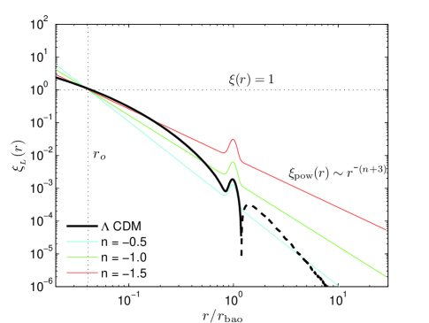
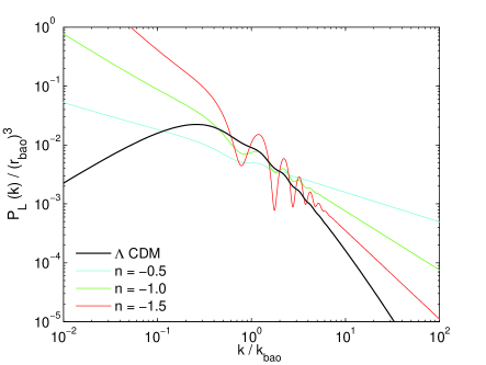
In Fig. 1 we compare the three different $\xi_{\,\rm{IC}}(r)$ models explored in this paper (blue, green, and red) to a standard $\Lambda$CDM correlation function (black). We show the fourier transform of these correlation functions – the resultant $P_{\rm{IC}}(k)$ – in Fig. 2 compared to a flat $\Lambda$CDM power spectrum generated from CAMB (Lewis et al., 2000) assuming fiducial WMAP7 parameters (Komatsu et al., 2011). In keeping with convention, we refer to the powerlaw in fourier space ($n=-0.5,-1.0,-1.5$) rather than in configuration space. These choices for the powerlaw slope are inspired by the resemblance to the $\Lambda$CDM correlation function on different scales. Similarly, unless otherwise noted, we choose $\sigma_{\rm{bao}}=0.075\,r_{\rm{bao}}$ as the $\Lambda$CDM-inspired gaussian width and $A_{\rm{bump}}=2.75$ as the gaussian amplitude of the BAO feature.

In this study our time variable is $r_{0}/r_{\rm{bao}}$, where $\xi_{L}(r_{0})\equiv 1$. This quantity grows as the amplitude of $\xi_{L}(r)$ becomes larger and the correlation length $r_{0}$ increases. For convenience we show conversions between this convention for the non-linear scale and other choices in Table 1. Other popular conventions define the non-linear scale as $\sigma(R_{*})\equiv 1$ or $\sigma(R_{*})\equiv\delta_{c}$, i.e. the scale where the rms density in spheres reaches one or reaches the threshold for spherical collapse, $\delta_{c}=1.69$. We show $R_{*}/r_{\rm{bao}}$ for $\sigma(R_{*})\equiv 1$ in the second column in Table 1; to convert from $\sigma(R_{*})\equiv 1$ to $\sigma(R_{*})\equiv\delta_{c}$, multiply this column by $\delta_{c}^{2/(n+3)}$. A fourier-space convention for the non-linear wavenumber, $\Delta^{2}(k_{\rm{NL}})\equiv 1$ where $\Delta^{2}(k)=k^{3}P(k)/(2\pi)^{3}$, is also shown in the third column. $k_{\rm{NL}}$ is shown divided by $k_{\rm{bao}}=2\pi/r_{\rm{bao}}$ so as to be independent of a specific choice of $r_{\rm{bao}}$ and to reflect the self-similar nature of the setup. Finally, the fourth column shows the effective value of $\sigma_{8}$, computed assuming $r_{\rm{bao}}=100\,h^{-1}\rm{Mpc}$. More generally this column can be interpreted to be the rms density contrast in spheres of radius 8% of the BAO scale.

We begin our simulations at the earliest epoch listed for each of the three models shown in Table 1, and we obtain outputs at each of the epochs listed.

Table 1: Normalization/Conversion Table

	$r_{0}/r_{\rm{bao}}$	$R_{*}/r_{\rm{bao}}$	$k_{\rm{NL}}/k_{\rm{bao}}$	$\sigma_{8}$
	0.00039	0.0073	34.1	0.05
	0.024	0.046	5.40	0.5
	0.043	0.080	3.10	1.0
	0.059	0.111	2.24	1.5
n = -0.5	0.074	0.139	1.78	2.0
	0.102	0.193	1.02	3.0
	0.129	0.243	0.856	4.0
	0.178	0.335	0.740	6.0
	0.311	0.584	0.588	12.0
	0.0027	0.0040	41.2	0.05
	0.027	0.040	4.12	0.5
	0.043	0.064	2.58	0.8
	0.053	0.080	2.06	1.0
	0.073	0.110	1.51	1.37
n = -1	0.080	0.120	1.37	1.5
	0.107	0.160	1.03	2.0
	0.160	0.240	0.687	3.0
	0.213	0.320	0.515	4.0
	0.267	0.400	0.412	5.0
	0.320	0.480	0.258	6.0
	0.0011	0.0015	56.6	0.05
	0.024	0.032	2.63	0.5
	0.061	0.080	1.04	1.0
n = -1.5	0.104	0.137	0.608	1.5
	0.153	0.202	0.414	2.0
	0.263	0.346	0.241	3.0
	0.386	0.508	0.164	4.0

II.2 Approximate Solution for $P_{IC}(k)$

Starting from the fourier transform relation,

$$P_{\rm{IC}}(k)=4\pi\int_{0}^{\infty}\xi_{\rm{\,IC}}(r)\,\frac{\sin(kr)}{kr}\,r^{2}\,{dr},$$ (3)

and breaking up $\xi_{\rm{IC}}(r)$ in Eq. 1 into two terms, we expect

$$P_{\rm{IC}}(k)=P_{\rm{pow}}(k)+P_{\rm{wig}}(k).$$ (4)

An exact analytic solution exists for the powerlaw term (Peebles, 1980): the fourier transform of $P_{\rm{pow}}=Aa^{2}k^{n}$ is $\xi(r)=(r_{0}/r)^{n+3}$ with amplitudes related by

$$A\,a^{2}=\frac{2\pi^{2}\,\,\,(2+n)}{\Gamma(3+n)\sin((2+n)\pi/2)}r_{0}^{n+3}\equiv A_{n}r_{0}^{n+3}.$$ (5)

The remaining $P_{\rm{wig}}(k)$ term in Eq. 4 is given by

$$\begin{array}[]{l l}\displaystyle P_{\rm{wig}}(k)&=\displaystyle\frac{4\pi A_{\rm{bump}}r_{0}^{\gamma}}{k}\times\\ &\displaystyle\int^{\infty}_{0}{r^{-(n+2)}e^{-(r-r_{\rm{bao}})^{2}/2\sigma_{\rm{bao}}^{2}}\,{\rm sin}(kr)}{\,dr}~{}.\end{array}$$ (6)

Up to a normalization, the integral is simply the expectation value of $r^{-(n+2)}\sin kr$ over a gaussian probability distribution $p(r)$ centered on $r_{\rm{bao}}$ with width $\sigma_{\rm{bao}}$ (but truncated at $r>0$):

$$\int^{\infty}_{0}{r^{-(n+2)}\,{\sin(kr)}\,p(r)\,}{dr}\approx(2\pi\sigma_{\rm{bao}}^{2})^{1/2}\langle\,r^{-(n+2)}\ {\sin(kr)}\,\rangle.$$ (7)

Since $p(r)$ is strongly peaked at $r=r_{\rm{bao}}$, and since $\sin(kr)$ is generally much more sensitive than $r^{-(n+2)}$ to the value of $r$, we have, to good approximation,

$$\langle r^{-(n+2)}\,{\rm sin}(kr)\rangle\approx\langle r^{-(n+2)}\rangle\langle{\rm sin}(kr)\rangle\approx r_{\rm{bao}}^{-(n+2)}\langle{\rm sin}(kr)\rangle,$$ (8)

leaving only the expectation value of $\sin(kr)$ to be determined. This expression is given by

$$\langle\,{\rm sin}(kr)\,\rangle=(2\pi\sigma_{\rm{bao}}^{2})^{-1/2}\int^{\infty}_{0}{e^{-(r-r_{\rm{bao}})^{2}/2\sigma_{\rm{bao}}^{2}}\,{\rm sin}(kr)}{\,dr}$$

$$\approx{\rm sin}(kr_{\rm{bao}})\,{\rm exp}(-(k\,\sigma_{\rm{bao}})^{2}/2).\;\;\;\;\;\;\;\;\;\;\;\;\;\;\;\;\;\,$$ (9)

This line of approximation ultimately leads to

$$P_{\rm{IC}}(k)\ \approx\ \ A_{n}r_{0}^{3}\,(kr_{0})^{n}\ \ +\;\;\;\;\;\;\;\;\;\;\;\;\;\;\;\;\;\;\;\;\;\;\;\;\;\;\;\;\;\;\;\;\;\;\;\;\;\;$$ (10)

$$2^{5/2}\pi^{3/2}A_{\rm{bump}}\sigma_{\rm{bao}}r_{\rm{bao}}^{2}\bigg{(}\frac{r_{0}}{r_{\rm{bao}}}\bigg{)}^{n+3}\frac{{\rm sin}(kr_{\rm{bao}})}{kr_{\rm{bao}}}e^{-k^{2}\sigma_{\rm{bao}}^{2}/2}.$$

With our $\Lambda$CDM-inspired choices for the constants in this expression (discussed in § II.1), our approximation for $P_{\rm{IC}}(k)$ agrees with the numerical integration to better than a percent (relative to the underlying powerlaw) over the entire range of $k$-values.

II.3 Integration of Particle Trajectories

We used the publicly-available Gadget2 code (Springel, 2005) to integrate particle trajectories from the initial conditions. Gadget2 is a hybrid, Tree-PM code in which the long-range gravitational forces are computed by solving the Poisson equation in fourier space while the short range forces are computed using a Tree algorithm (Barnes and Hut, 1986). Gadget2 is parallelized using standard MPI and allocates processors/cores with the space-filling Peano-Hilbert curve. This allows the code to perform well on massively-parallel machines.

Throughout, unless otherwise noted, we simulate the powerlaw times a gaussian model using a flat $\Omega_{m}=1.0$ cosmology with no dark energy, much like in self-similar pure powerlaw investigations (e.g. Efstathiou et al., 1988; Widrow et al., 2009) or in cCDM (Carlson et al., 2009; Padmanabhan and White, 2009). This choice allows structure to grow indefinitely, avoiding the freeze-out limit when the dark energy component comes to dominate. However, in § IV.2, we present some simulations that include a cosmological constant and conclude that the evolution of the bump still only depends on the ratio of the non-linear scale to the BAO scale, even when dark energy is present.

Most of the simulations presented here, unless otherwise noted, were run with $512^{3}$ particles using a $768^{3}$ PM grid for the large scale forces and a comoving force softening (relevant to the tree part of the code) of 1/4th the initial mean interparticle spacing. Our box size was chosen to be $\sim$20$\times$ larger than the BAO scale, making the force softening $\sim$1/2000th the scale of the box. We ran seven realizations of each model in order to obtain better statistics on large scales. We also performed pure powerlaw simulations (i.e. no wiggles) with the three cases ($n=-0.5$, $n=-1$, $n=-1.5$) to compare with the cases that include a BAO feature (Appendix A). Also note that we apply a correction to $\xi_{\rm{meas}}(r)$ to account for the artificial enforcement of the integral constraint on $\xi_{\rm{meas}}(r)$ (Appendix B). This correction is important on large scales for $n\leq-1$.

The simulations were evolved to the point where the non-linear scale reached approximately 30% of the initial BAO scale. As in pure powerlaw simulations, there is a concern that for steep power spectra the missing power on scales larger than the box will invalidate the results. However, even in the last output of the $n=-1.5$ case, which has the most large scale power, our simulations fall well within the guidelines recommended by Smith et al. (2003), and the self-similarity of the pure powerlaw results in Appendix A seem also to confirm the validity of our simulation results.

All of the simulations presented here were performed using the Glenn cluster at the Ohio Supercomputer Center. In total, the results in this paper are based on 28 $512^{3}$-particle simulations of powerlaw+bump initial conditions, 21 $256^{3}$-particle simulations and 28 $512^{3}$-particle simulations used in the tests of IV, and 20 $512^{3}$-particle simulations of pure powerlaw models presented in Appendix A.

III Evolution of the BAO Bump

Figure 3: Matter 2-point correlation function results for a powerlaw times a gaussian model for dark matter clustering. The upper two panels show results for the $n=-0.5$ background powerlaw, while the middle two panels show $n=-1$ and the lower two $n=-1.5$. The left panels show the measured matter autocorrelation function from the simulations at various epochs as colored points and, in dashed lines with the same color scheme, the corresponding linear theory correlation function at each epoch. The right panels show the matter autocorrelation function divided by the pure powerlaw correlation function, $\xi_{\rm{pow}}(r)$. Black dashed lines show the linear theory prediction, which is independent of epoch. Typical errors on the mean for $\xi_{\rm{meas}}(r)/\xi_{\rm{pow}}(r)$ are shown off to the right for various epochs, but note that errors are strongly correlated across the full range of the bump. On the right hand panels we also overplot with dot-dashed lines the best fit gaussians with the same color scheme as the measurements from simulations. $\xi(r)$ has been corrected for the integral constraint as described in Appendix B. Comparable plots for a $\Lambda$CDM power spectrum appear in Fig. 15

III.1 $\xi(r)$ results for fiducial case

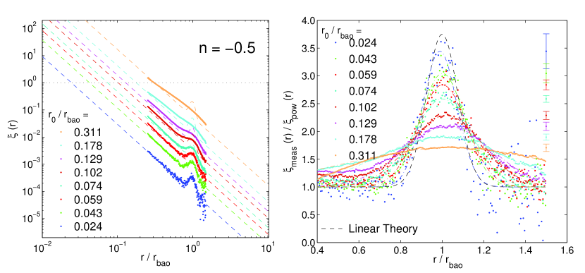
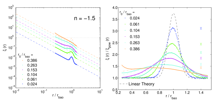
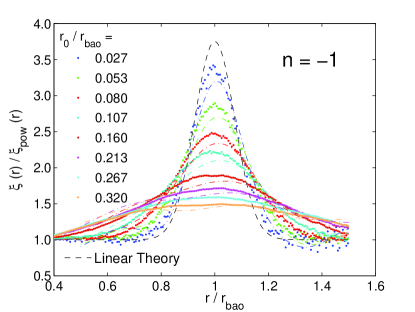
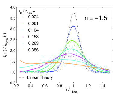
Fig. 3 presents our main results for the configuration-space evolution of the BAO feature. Remarkably, when divided by the pure powerlaw correlation function as in the plots on the right hand column, the BAO feature maintains a gaussian shape throughout the non-linear broadening and damping that occurs in structure formation. In linear theory the bump would maintain the initial shape as indicated with the black dashed lines on the right hand column.

We overplot the best fit gaussians on the right hand column with dot-dashed lines of various colors corresponding to different epochs to emphasize and better illustrate this gaussian behavior. We consider quantitative measures of the evolution in bump amplitude and width in § III.3.

When comparing the three models, one should bear in mind that at fixed $r_{0}/r_{\rm{bao}}$ the bump in the $n=-0.5$ case is at a much lower clustering amplitude than in the $n=-1.5$ case simply because an $n=-1.5$ powerlaw has much more large scale power, and we defined the initial bump feature to be a gaussian times (rather than added to) a powerlaw. The simulation data for the $n=-0.5$ case are noisier, especially at early epochs, because we are measuring a weaker signal.

Figure 4: Results for a setup where the initial gaussian width of the bump is half of its fiducial value and the background powerlaw is set to $n=-1$. As in Fig. 3 different outputs are shown in different colors, with the typical errors on the mean offset to the right. $\xi(r)$ has been corrected for the integral constraint as described in Appendix B.

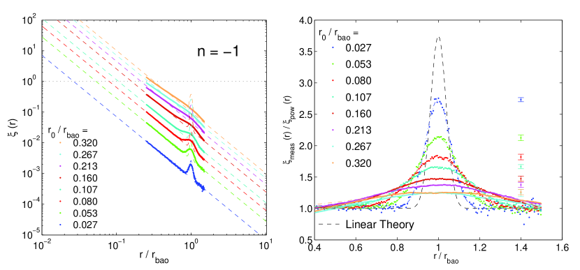
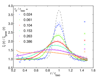
The other striking feature of Fig. 3 is that the location of the bump maximum stays nearly fixed in the $n=-0.5$ and $n=-1$ cases, even when they are evolved to high values of $r_{0}/r_{\rm{bao}}$ (corresponding to $\sigma_{8}=6-12$), while the location of the maximum for the $n=-1.5$ case shifts substantially at late times. The shifts for $n=-1.5$ are 6, 14, and 29 % at $r_{0}/r_{\rm{bao}}=$ 0.153, 0.263, 0.386 (corresponding to $\sigma_{8}=$ 2, 3, 4). By contrast, in $\Lambda$CDM one typically sees shifts of $\sim 0.5\%$ by $z=0$ ($\sigma_{8}\approx 0.8$), and extrapolating the fitting formula of Seo et al. (2010) to an extreme value of $\sigma_{8}=D(z)/D(0)\approx 4$ predicts a shift of only $\sim 5\%$. Qualitatively, we can understand the different behavior of $n=-1.5$ as a consequence of the much higher clustering amplitude at $r\approx r_{\rm{bao}}$ (see Fig. 1). We will discuss the non-linear shift of the BAO peak in further detail in following sections.

As one last qualitative note on the $n=-1.5$ results in Fig. 3, at the two latest epochs one can see that the correlation function at $r\sim 0.5r_{\rm{bao}}$ is showing significant non-linear evolution away from the initial power-law, in contrast to the other two cases. We avoid this region in determining the best fit gaussians to the simulation data.

III.2 Evolution of a “Skinny” Bump

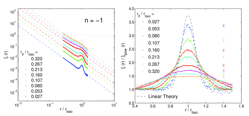
We also investigated a case where the initial gaussian width of the bump was half of the value in the fiducial case, i.e. $\sigma_{\rm{bao}}=0.0375\,r_{\rm{bao}}$ instead of the $\Lambda$CDM-inspired value of $\sigma_{\rm{bao}}=0.075\,r_{\rm{bao}}$. Keeping $A_{\rm{bump}}$ fixed at 2.75, we performed simulations only for the $n=-1$ background powerlaw. These results are shown in Fig. 4. The bump clearly maintains a gaussian shape as it is damped out, and, as in the fiducial $n=-1$ case, there does not seem to be any shift in the BAO peak by the end of the simulation.

III.3 Quantitative Characterization of the Bump Evolution

Figure 5: Results for the dimensionless width (top), amplitude (middle), and a proxy of the dimensionless area under the bump (lower panel). Overplotted in the top two panels is a diffusion model in which the broadening of the width scales as suggested by the rms pairwise displacement equation (Eq. 11) while the area of the gaussian bump is held constant. The diffusion constant is predicted ab initio for $n=-1.5$ and chosen by visual fit to the data points for $n=-1$ and $n=-0.5$. Error bars are from jackknife error estimation.

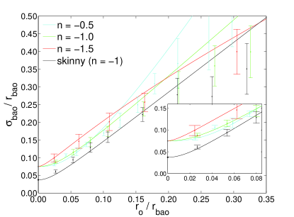
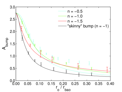
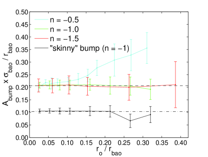
In Figs. 5 and 6 we plot evolution of the amplitude, width, and peak location measured from gaussian fits to our simulation results. These gaussian functions were determined by first making a rough determination of the BAO peak and bump amplitude from $\xi(r)/\xi_{\rm{pow}}(r)$, then varying $r_{\rm{bao}}$, $A_{\rm{bump}}$ and $\sigma_{\rm{bao}}$ in a 3-dimensional $\chi^{2}$ to find the best fit. This minimization was done using $\xi(r)/\xi_{\rm{pow}}(r)$ as in the right hand panels of Fig. 3 rather than $\xi(r)$ itself. We avoided correlation function data more than $\Delta r\sim 0.3r_{\rm{bao}}$ below the peak in finding the best fit gaussian, to avoid effects of non-linear evolution of the underlying powerlaw correlation function. Error bars in Figs. 5 and 6 were determined via jackknife error estimation by sequentially omitting the correlation function results for one of the seven realizations and determining the best fit gaussians in each case. The errors on $A_{\rm{bump}}\times\sigma_{\rm{bao}}/r_{\rm{bao}}$, a dimensionless proxy for the area of the bump, are from propagated errors in the values of $A_{\rm{bump}}$ and $\sigma_{\rm{bao}}$. The $n=-1.5$ case suffers from a slight degeneracy between the amplitude of the bump and the magnitude of the non-linear shift, so the jackknife error bars are slightly larger in this case.

Fig. 5 shows our main results for the quantitative evolution of the dimensionless bump width, $\sigma_{\rm{bao}}/r_{\rm{bao}}$, bump amplitude, $A_{\rm{bump}}$, and area $A_{\rm{bump}}\times\sigma_{\rm{bao}}/r_{\rm{bao}}$. In the top panel, in all cases there is significant broadening of the bump, while in the middle panel, even apart from the dot-dashed models which will be discussed in a moment, the amplitude of the $n=-0.5$ case appears to decrease more slowly than that of the other setups.

The lower panel of Fig. 5 shows that the area under the bump stays remarkably constant, closely following the black horizontal dashed and dot-dashed lines as the bump broadens and attenuates. We speculate that the non-linear dynamics of the growth of structure is just diffusively moving apart the pairs at separation $r\sim r_{\rm{bao}}$ so that $\sigma_{\rm{bao}}^{2}\approx\sigma_{\rm{IC}}^{2}+\sigma_{\rm{diff}}^{2}$, where $\sigma_{\rm{IC}}$ is the initial bump width and $\sigma_{\rm{diff}}$ is the rms broadening from this diffusion process, while the area under the bump stays constant and the gaussian shape is maintained. These assumptions underlie the models plotted in the top two panels of Fig. 5. The broadening is modeled by identifying $\sigma_{\rm{diff}}^{2}$ with the linear theory equation for the mean-squared relative displacement between pairs (Eq. 9 from Eisenstein et al., 2007),

$$\Sigma_{\rm{pair}}^{2}=r_{12}^{2}\int_{0}^{\infty}\frac{k^{2}dk}{2\pi^{2}}P(k)f_{||}(kr_{12}),$$ (11)

where $r_{12}$ is the separation and

$$f_{||}(x)=\frac{2}{x^{2}}\left(\frac{1}{3}-\frac{\sin(x)}{x}-\frac{2\cos(x)}{x^{2}}+\frac{2\sin(x)}{x^{3}}\right).$$ (12)

In the limit $r_{12}\rightarrow\infty$, Eq. 11 reduces to Eq. 2, i.e., the rms pairwise displacement $\Sigma_{\rm{pair}}$ asymptotes to the Zel’dovich displacement. However, modes with $kr_{12}\ll 1$ move pairs of particles separated by $r_{12}$ coherently, and while these modes may dominate the “bulk flow” they cannot affect clustering on scales $<r_{12}$. Notably, Eq. 2 is infrared divergent for $n\leq-1$, while Eq. 11 is IR convergent for $n>-3$, failing only when the density contrast (not peculiar velocity) has a divergent large scale contribution.

If, as an approximation to our model, we consider a pure powerlaw power spectrum, $P(k)\approx Aa^{2}k^{n}$, Eq. 11 can be re-written as

$$\Sigma_{\rm{pair}}^{2}=\frac{A\,a^{2}}{r_{12}^{n+1}}\frac{1}{2\pi^{2}}\int_{0}^{\infty}x^{2+n}f_{||}(x){dx},$$ (13)

where $x=kr_{12}$. Selecting $r_{12}=r_{\rm{bao}}$, and utilizing $Aa^{2}\sim r_{0}^{n+3}$ (Eq. 5), this implies a scaling of the form

$$\Sigma_{\rm{pair}}^{2}\sim r_{\rm{bao}}^{2}\left(\frac{r_{0}}{r_{\rm{bao}}}\right)^{n+3}.$$ (14)

The width of the bump can therefore be modeled with

$$\begin{array}[]{c c}\displaystyle\sigma_{\rm{bao}}^{2}=\sigma_{\rm{IC}}^{2}+\Sigma_{\rm{pair}}^{2},\\ \displaystyle\sigma_{\rm{bao}}^{2}=\sigma_{\rm{IC}}^{2}+2\,\kappa_{n}\,r_{\rm{bao}}^{2}\left(\frac{r_{0}}{r_{\rm{bao}}}\right)^{n+3}.\end{array}$$ (15)

We use the symbol $\kappa_{n}$ and include a factor of 2 to emphasize our characterization of the bump evolution as a diffusion process. For $-3<n<-1$, evaluating the integral in Eq. 13 yields an ab initio prediction for $\kappa_{n}$ (from $\Sigma_{\rm{pair}}^{2}$) of

$$\kappa_{n}=\frac{2+n}{2-n}\frac{\Gamma(1+n)}{\Gamma(3+n)}\frac{\sin(n\pi/2)}{\sin((2+n)\pi/2)}.$$ (16)

For shallower power spectra, $n\geq-1$, both Eq. 13 and Eq. 2 are UV divergent and $\kappa_{n}$ is undefined. In Fig. 5 we therefore model the evolution of $\sigma_{\rm{bao}}$ for $n=-0.5$ and $n=-1$ by assuming the scaling in Eq. 14 and empirically fitting $\kappa_{n}$ to our simulation results. For $n=-1.5$, Eq. 16 yields $\kappa_{-1.5}=4/7$.

The curves in the upper panel of Fig. 5 compare Eq. 15 with values of $\kappa_{n}=\{4.5,1.3,4/7\}$ for $n=-0.5,-1$ and $-1.5$, respectively, to the measurements from simulations. The $\kappa_{n}$ values for $n=-0.5$ and $-1$ were chosen by a visual fit to the simulation points, while $\kappa_{-1.5}$ is predicted ab initio. The model provides a good match to the data for $r_{0}/r_{\rm{bao}}<0.1$. Most significantly, the same $\kappa_{n}$ fits both the fiducial and skinny $n=-1$ cases, supporting the conjecture that the bump width is effectively set by a quadrature sum of the linear theory “intrinsic” width and the rms pairwise displacement (Eq. 15). The scaling with rms displacement holds fairly accurately out to large $r_{0}/r_{\rm{bao}}$. For comparison with an analogous test in $\Lambda$CDM, Fig. 3 of Eisenstein et al. (2007) shows that Eq. 11 accurately predicts the rms displacement of pairs initially separated by $r=100h^{-1}$ Mpc. This agreement extends to late times where the rms displacement has reached $\sim 8\%$ of this initial separation. The $n=-1.5$ results in the upper panel of Fig. 5 suggest that Eq. 11 is accurate (i.e. within errors) for rms displacements as large as $\sim 15\%$ of the scale of the initial separation.

The bottom panel of Fig. 5 shows that the constant-area approximation holds well for $n=-1$ and $n=-1.5$, but it breaks down for $n=-0.5$ when $r_{0}/r_{\rm{bao}}\gtrsim 0.1$. This lack of constant-area behavior for $n=-0.5$ at late times explains the divergence of points and model curve in the middle panel of Fig. 5.

Figure 6: Results for the non-linear shift of the BAO peak measured from the right panels of either Fig. 3 or Fig. 4. The “skinny” bump results are offset to the left by $\Delta r_{0}/r_{\rm{bao}}=0.01$ so as to avoid overlap with the fiducial $n=-1$ results. Dashed lines show a prediction for the shift of the peak based on Eq. 32 from Smith et al. (2008). Error bars are from jackknife error estimation.

Figure 7: Residuals showing the non-linear shift from subtracting the gaussian fits centered on the un-shifted BAO scale from the matter correlation function results from the first two outputs in the $n=-1.5$ case (blue and green points). The solid lines show the predictions of the Crocce and Scoccimarro (2008) ansatz in this case using $A_{\rm{mc}}=34/21$ for both outputs. The thin green-dashed line uses this ansatz but assumes a broadened and attenuated bump in $\xi_{\rm{mc}}(r)$ as discussed in the text.

III.4 Movement of the BAO peak

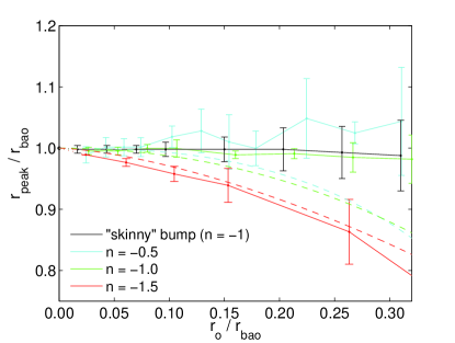
Fig. 6 shows the change in position of the bump maximum, determined as described in § III.3 by fitting a gaussian to the ratio of the non-linear correlation function to the linear-theory powerlaw. As already noted in our discussion of Figs. 3 and 4, there is no significant shift of the peak location on our simulations for either the $n=-0.5$ or $n=-1$ cases (fiducial or “skinny” bump). Error bars on the $n=-0.5$ peak location become large at late times because the bump itself flattens and the large scale correlation is weak. For $n=-1$, the skinny bump errors are initially lower than those of the fiducial model because the sharper peak can be centroided more precisely, but they are higher at late times because the skinny bump gets depressed to a lower amplitude. In contrast to the other cases, the $n=-1.5$ model shows significant and strong peak shifts, evident already for $r_{0}/r_{\rm{bao}}=0.024$ ($\sigma_{8}=0.5$). Indeed, we have truncated the plot before the final $n=-1.5$ output, with $r_{0}/r_{\rm{bao}}=0.386$ and $r_{\rm{peak}}/r_{\rm{bao}}=0.71$.

We compare these results to an elegant model for the shift from Smith et al. (2008) that uses linear theory velocities and the pair-conservation constraint on $\xi(r)$ to track the average motion of pairs separated by $r_{\rm{bao}}$. Their equation (32) can be written

$${D^{2}(z)\over D_{\rm{ic}}^{2}}-1=\int_{r_{\rm{peak}}}^{r_{\rm{bao}}}\frac{3}{\bar{\xi}_{\rm{ic}}(r)}\frac{dr}{r}~{},$$ (17)

where $D(z)$ is the linear growth factor, the subscript ic refers to initial conditions when fluctuations are fully in the linear regime, $r_{\rm bao}$ is the linear theory BAO position, $r_{\rm peak}$ is the non-linear position of the peak, and $\bar{\xi}(r)$ is the volume-averaged correlation function interior to radius $r$. For $D(z)/D_{\rm ic}\gg 1$ and our initial conditions, this equation leads to the approximate result

$$\frac{r_{\rm{peak}}}{r_{\rm{bao}}}\approx\left[1+\frac{n+3}{n}C_{n}\left(\frac{r_{0}}{r_{\rm{bao}}}\right)^{n+3}\right]^{1/(n+3)}~{},$$ (18)

where $C_{n}$ would be 1.0 for a pure powerlaw spectrum and incorporating the bump gives $C_{n}\approx\{1.13,1.26,1.38\}$ for $n=\{-0.5,-1,-1.5\}$. For $n<0$ this formula predicts that the peak shifts to smaller scales. In the limit of small $r_{0}/r_{\rm bao}$, a binomial expansion yields

$$\frac{r_{\rm{peak}}}{r_{\rm{bao}}}\approx 1+\frac{C_{n}}{n}\left(\frac{r_{0}}{r_{\rm{bao}}}\right)^{n+3}~{}.$$ (19)

Since $r_{0}^{n+3}\propto D^{2}(z)$, the non-linear shift grows as the square of the linear growth function as expected from PT (e.g. Padmanabhan and White, 2009; Seo et al., 2010), and the displacement is larger for more negative $n$.

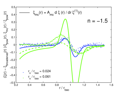
The seemingly quite different argument of Crocce and Scoccimarro (2008) leads to a similar expression for the peak shift. They propose modeling the non-linear correlation function in the neighborhood of the bump by

$$\xi_{\rm{NL}}(r)\approx\xi(r)+A_{\rm mc}\frac{d\xi(r)}{dr}\,\frac{r\,\bar{\xi}(r)}{3}~{},$$ (20)

where the mode-coupling factor $A_{\rm mc}$ can be treated as a fitting parameter but the value $34/21$ obtained from PT is in fact close to the best-fit numerical value (see Crocce et al. (2011), Appendix A). With judicious use of Taylor expansions in the limit of small shift and minimal non-linear broadening, one can derive

$$\frac{r_{\rm{peak}}}{r_{\rm{bao}}}\approx 1+\frac{34}{21}\frac{C_{n}}{n}\left(\frac{r_{0}}{r_{\rm{bao}}}\right)^{n+3}~{},$$ (21)

hence a shift about 50% larger than Eq. (19) but with the same dependence on $r_{0}$ and $n$.

Dashed lines in Figure 6 show the prediction of Eq. (19). The model correctly predicts that the shift is much larger for $n=-1.5$ than for $n=-1$ or $n=-0.5$. For $n=-1.5$, it tracks the numerically measured shift remarkably well. For the other $n$ values, it predicts too large a shift for $r_{0}>0.1r_{\rm bao}$; at smaller $r_{0}$, the model is consistent with the numerical results within the error bars, but the numerical results are also consistent with zero shift. We note that our treatment does not include the 1-loop PT extension of Smith et al. (2008)’s model, which could improve agreement at later epochs.

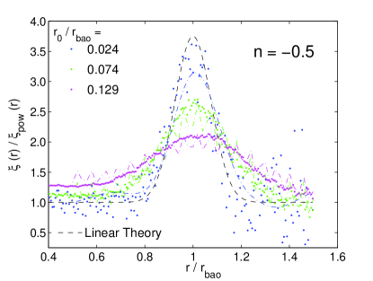
Figure 7 compares Eq. (20) to the first two outputs of the $n=-1.5$ simulations. For $r_{0}/r_{\rm bao}=0.024$, this model predicts the distortion in the neighborhood of the peak remarkably well, with no free parameters. Note that there is a clear non-linear shift of the peak at this output, despite the low value of $\sigma_{8}=0.5$. For $r_{0}/r_{\rm bao}=0.061$, the model predicts too large a distortion. However, if we insert the broadened and lower amplitude bump (taking $\sigma_{\rm bao}$ and $A_{\rm bump}$ from the model discussed in the previous section) into the calculation of Eq. (20), an approach that seems reasonable but is not rigorously justified, then we get the dashed green lines in Figure 7, which agrees much better (though not perfectly) with the numerical results.

We conclude that these analytic approaches can explain why the shift in the bump location is much larger for $n=-1.5$ and can capture at least some of the quantitative behavior of the peak shift. However, they do not work accurately over a wide range of $r_{0}/r_{\rm bao}$ and $n$. We will return to the comparison of PT predictions and our numerical results in §V, in the context of the power spectrum.

IV Self-Similar Tests

Figure 8: Tests of robustness to numerical parameters. (Top ) Comparison of the bump region of $\xi(r)$ in simulations with $r_{\rm{bao}}/L_{\rm{box}}=1/10$ (points) to the gaussian fits (lines) from the fiducial simulations in Fig. 3, which have $r_{\rm{bao}}/L_{\rm{box}}=1/20$. (Bottom) Comparison of simulations with $r_{\rm{bao}}/L_{\rm{box}}=1/20$ but $256^{3}$ particles, hence $r_{\rm{bao}}/n_{p}^{-1/3}=12.5$, to the fiducial simulations with $512^{3}$ particles and $r_{\rm{bao}}/n_{p}^{-1/3}=25$.

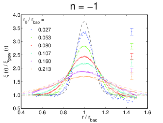
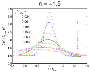
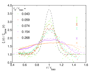
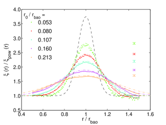
In an $\Omega_{m}=1$ pure powerlaw model, i.e. $P(k)=Ak^{n}$, since the only scale germane to the problem is the amplitude, $A$, the evolution of clustering statistics should depend only on the value of $A$ or some derived variable such as $k_{\rm{NL}}=(2\pi^{2}/A)^{1/(n+3)}$. The evolution may be different for each powerlaw but with $n$ fixed there should be a unique function (e.g. of $k/k_{\rm{NL}}$, or $r/R_{\rm{NL}}$, or $M/M_{\rm{NL}}$, …) that fully describes any given clustering statistic, even well into the non-linear regime. In the early days of cosmological N-body investigations, demonstrations of self-similar evolution with pure powerlaw cosmologies, in addition to providing physical insight, also gave decisive confirmations of the accuracy of simulations (e.g. Efstathiou et al., 1988; Bertschinger and Gelb, 1991; Lacey and Cole, 1994; Jain et al., 1995; Colombi et al., 1996). We take advantage of the simplicity of the powerlaw times a gaussian setup to perform self-similar tests that can be used in an analogous way to test the accuracy of the simulations on the scale of the bump.

The powerlaw times a bump setup clearly has two scales at play instead of one, so in this case, for a given powerlaw and a given initial bump width, the non-linear dynamics should evolve only as a function of the ratio of the non-linear scale to the BAO scale. The dynamics are self-similar in the sense that any property of the system, such as the broadening of the bump or the shift in the peak for a particular powerlaw, is determined by how close the non-linear scale, $r_{0}$, has come to the BAO scale. Unlike a $\Lambda$CDM simulation the result should not, in principle, depend on whether the bump is initially set at, e.g., 100 $h^{-1}~{}\rm{Mpc}$ or 130 $h^{-1}~{}\rm{Mpc}$; only the ratio of the non-linear scale to the BAO scale matters in determining the evolution. If the N-body results do depend, separately, on the BAO scale or the non-linear scale, this can be interpreted as a sign of numerical artifacts.

IV.1 Robustness to Varying Box Size and Mean Interparticle Spacing

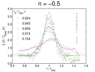
Cosmological N-body simulations unavoidably introduce two artificial scales into the problem – the box size, $L_{\rm{box}}$, and the initial mean interparticle spacing, $l_{p}=n_{p}^{-1/3}=L_{\rm{box}}/N^{1/3}$. Both of these scales can potentially interfere with the evolution of the BAO feature and bias one’s results. In the upper panels of Fig. 8 we show results from tests where the BAO scale has been doubled (or equivalently the box-size halved), such that $r_{\rm{bao}}/L_{\rm{box}}\approx 1/10$ instead of the fiducial value of $r_{\rm{bao}}/L_{\rm{box}}\approx 1/20$ in the simulations shown elsewhere in the paper. The number of particles in this test is kept fixed at $512^{3}$, so that the ratio of the BAO scale to the mean interparticle spacing increases from $r_{\rm{bao}}/n_{p}^{-1/3}=25$ (as in the fiducial simulations) to $50$. We also show tests (lower three panels) where the box size is kept fixed while the number of particles is decreased to $256^{3}$, arguably more akin to a conventional convergence test. Each panel in Fig. 8 shows the results from seven realizations (as in the fiducial simulation set), and in each panel we plot the best-fit gaussians from our fiducial set of simulations (dot-dashed lines). Note that for the “double-the-bump” tests in the upper panels of Fig. 8, these simulations had to be run for much longer than in the fiducial case in order for the non-linear scale to approach the BAO scale, which had been placed at twice the fiducial separation.

To the extent that the simulations in Fig. 8 match the fit from the fiducial set of simulations, the evolution can be said to be self-similar and unaffected by the artificially-introduced numerical scales. For the double-the-bump tests, the results seem to match the fiducial simulations well. In this case, especially for $n=-1.5$, the integral-constraint correction to $\xi(r)$ discussed in Appendix B is critical. We interpret this agreement as an indication that $r_{\rm{bao}}/L_{\rm{box}}\lesssim 1/10$ is acceptable if one includes integral-constraint corrections. Note that the measured errors on the mean are larger for these tests, which measure the correlation function on scales closer to the box scale than in the fiducial simulations. These larger errors are consistent with expectations from Gaussian statistics in a finite volume Cohn (2006).

The $256^{3}$ test was not quite as successful. The accelerated attenuation of the bump in the $n=-1.5$ case is severe enough to be of particular concern, especially since this setup is the one which actually sees an appreciable change in the BAO peak. The $n=-1$ simulations agree much better but still slightly underpredict the bump height. This also seems to be the case with the $n=-0.5$ results, which are more noisy. Though not quite a failure, we interpret this test to recommend keeping $r_{\rm{bao}}/n_{p}^{-1/3}\gtrsim 25$, as in our fiducial set of simulations.

The tests in Fig. 8 show that the evolution of the bump – its flattening, its movement in the $n=-1.5$ case, the lack of movement in the $n=-0.5$ and $-1$ cases, and the unexplained behavior of the bump area in the $n=-0.5$ case – is robustly predicted even when numerical parameters are changed substantially. For the wider importance of using BAO to constrain cosmology, this is an encouraging sign that modest N-body simulations can accurately render the non-linear shift of the BAO peak with very different models for the broad-band clustering. For power spectra that span a much wider range than $\Lambda$CDM models, numerical parameters $r_{\rm{bao}}/L_{\rm{box}}\lesssim 1/10$ and $r_{\rm{bao}}/n_{p}^{-1/3}\gtrsim 25$ appear to be adequate.

Figure 9: Results for a model including a cosmological constant ($\Omega_{m}=0.3,\,\Omega_{\Lambda}=0.7$ at the output with $r_{0}/r_{\rm{bao}}=0.043$) and with an $n=-1$ background powerlaw. The first and third outputs (blue and red) are directly comparable to the first and second outputs of the fiducial $n=-1$ simulations; thus the gaussian fits to those outputs in the fiducial case are overplotted. The second and last outputs (green and cyan) are compared to extrapolations from the fiducial $n=-1$ case assuming no non-linear shift and a model for the bump evolution as described in § III.3.

IV.2 A Test with Dark Energy

Even with a powerlaw initial spectrum, the introduction of dark energy in principle breaks self-similarity by defining a characteristic time (when $\Omega_{m}$ and $\Omega_{\Lambda}$ are equal), however in linear perturbation theory and the quasi-linear Zel’dovich and adhesion (Gurbatov et al., 1989; Weinberg and Gunn, 1990) approximations, evolution is determined only by the linear growth factor, with no direct dependence on $\rho_{m}(a)$ or $\rho_{\rm{DE}}(a)$. Zheng et al. (2002) and Nusser and Colberg (1998) demonstrate that this dependence on the linear growth factor alone remains a very good approximation in fully non-linear N-body simulations, the latter also showing explicitly that the full equations of motion for cosmological perturbations are weakly dependent on the individual values of $\Omega_{m}$ and $\Omega_{\Lambda}$ when those equations are expressed using the linear growth factor as the time variable. We may therefore expect self-similar evolution of the BAO bump as a function of $r_{0}/r_{\rm{bao}}$, even when dark energy is included.

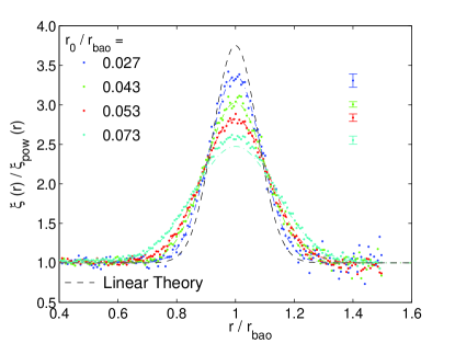
Fig. 9 compares these expectations to the N-body simulation results by presenting the evolved bump in a set of simulations ($n=-1$) that include a cosmological constant in comparison to the gaussian fits to our fiducial simulations. The simulation set has $\Omega_{m}=0.3,\Omega_{\Lambda}=0.7$ at output $r_{0}/r_{\rm{bao}}=0.043$. For some outputs, we have interpolated between outputs of our fiducial simulations assuming the model for the bump evolution discussed in § III.3. A substantive difference between $\Omega_{m}=1$ and dark energy models is that the growth of structure “freezes out” as dark energy becomes the dominant component of the universe. The last output in Fig. 9 is very close to this “freeze-out” limit in the linear theory growth function, which prevents $r_{0}/r_{\rm{bao}}$ from growing beyond 0.073 in this case.

The gaussian fits to the fiducial simulations agree well with the simulation results in Fig. 9, even for the last output which, with considerable computational expense, was evolved very close to the freeze-out limit. This confirms the expectations of self-similar evolution for this setup even in cosmologies with dark energy.

V Evolution of the BAO feature in Fourier Space

Figure 10: Left column: Measured power spectra for the fiducial $n=-0.5$ (top), $n=-1$ (middle) and $n=-1.5$ (bottom) simulations. The x-axis is shown normalized to the scale of the BAO feature, $k_{\rm{bao}}=2\pi/r_{\rm{bao}}$ and the y-axis is likewise shown as a dimensionless quantity, $P(k)/r_{\rm{bao}}^{3}$. There is no correction for shot noise; the shot noise level is indicated with dot-dashed lines. Right column: Results from dividing by the linear theory pure powerlaw. In both columns a phenomenological model (Eq. 22, solid colored lines) is compared to the simulation results. The scale corresponding to half the particle nyquist wavenumber is indicated with a vertical black dotted line.

V.1 Power Spectrum Estimation

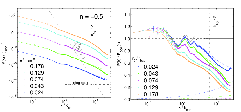
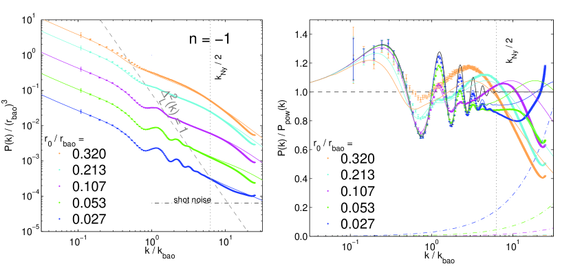
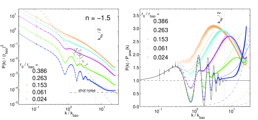
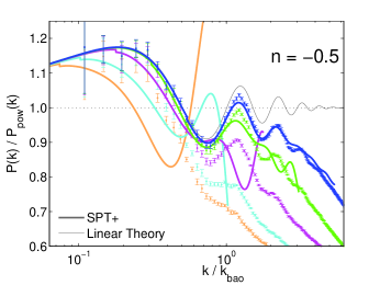
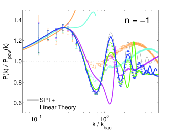
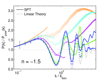
Power spectra were determined for the $n=-0.5,-1$ and $-1.5$ models by mapping the particles onto a $1024^{3}$ grid using the cloud in cell (CIC) assignment scheme. Performing a discrete fast fourier transform on this grid yields $\hat{\delta}(\vec{k})$ and fourier amplitudes $P(\vec{k})=|\hat{\delta}(\vec{k})|^{2}$. The artificial smoothing introduced by the griding scheme is corrected for by dividing $P(\vec{k})$ by the appropriate assignment function for CIC (Hockney and Eastwood, 1981), and the corrected $P(\vec{k})$ is binned in $k$ to yield $P(k)$. Following Heitmann et al. (2010) we do not include any kind of shot noise correction (e.g Jing, 2005; Colombi et al., 2009), and we follow their advice in trusting the computed power spectra only up to half the particle nyquist wavenumber, as indicated with black dotted vertical lines in Fig. 10, which presents our primary power spectrum results. The power spectrum up to this $k$-value should be negligibly affected by the aliasing of the $1024^{3}$ grid. Notwithstanding our conservative decisions in measuring $P(k)$, we will argue in the next section that a simple phenomenological model that draws on results from pure powerlaw simulations (Appendix A) allows our predictions to be extended to much higher $k$ for the early outputs.

We report power spectra throughout, normalizing the wavenumbers by $k_{\rm{bao}}=2\pi/r_{\rm{bao}}$, and giving the power spectrum amplitudes in terms of $P(k)/r_{\rm{bao}}^{3}$. This reflects the self-similar nature of the problem and allows more straightforward identification of the $k$-values of various nodes and anti-nodes. For technical reasons we throw out the measurements of the spectral power for $k\approx 2\pi/L_{\rm{box}}$, which should be computed separately from measurements at higher $k$ because of the different statistics of mode-counting near the scale of the box. The power on these scales is also inevitably noisy because of the small number of modes.

V.2 Interpretation

Ignoring the wiggles in Fig. 10 for a moment and focusing on the evolution of the overall shape of the power spectrum, the results are bracketed by the $n=-0.5$ spectrum, which trails behind the linear theory powerlaw at high $k$, and the $n=-1.5$ spectrum, which clearly outpaces the linear theory clustering prediction. This behavior is expected from perturbation theory (Scoccimarro and Frieman, 1996; Scoccimarro, 1997), and the trend is more clearly shown in the pure powerlaw plots in Appendix A. Physically, the behavior of the $n=-0.5$ powerlaw is sometimes described as “pre-virialization” (Davis and Peebles, 1977), where on small scales the clustering power is so high that as halos form they pull away from the expansion of the universe and the non-linear power spectrum falls behind the linear theory prediction. For much steeper powerlaws, like $n=-1.5$ or the high $k$ spectrum of $\Lambda$CDM, the trend is the opposite; clustering power is “transferred” from large scales to smaller scales. The $n=-1$ spectrum lies between these two extremes, and its spectrum is above and below the linear theory prediction in different ranges (Appendix A).

With this in mind we modeled the power spectrum results with a phenomenological approach, treating separately the non-linear evolution of the pure powerlaw spectrum and modeling the wiggles by coupling the analytic solution in Eq. 10 with the diffusion model introduced in § III.3. Thus, the model is

$$P_{\rm{phen}}(k)\ =\ \ A_{n}r_{0}^{3}(kr_{0})^{n}f_{n}(k/k_{\rm{NL}})\ \ +\;\;\;\;\;\;\;\;\;\;\;\;\;\;\;\;\;\;\;\;\;\;\;\;\;$$ (22)

$$2^{5/2}\pi^{3/2}A_{\rm{bump}}^{\prime}\sigma_{\rm{bao}}^{\prime}r_{\rm{bao}}^{2}\bigg{(}\frac{r_{0}}{r_{\rm{bao}}}\bigg{)}^{n+3}\frac{{\rm sin}(k\,r_{\rm{bao}}^{\prime})}{kr_{\rm{bao}}^{\prime}}e^{-k^{2}\sigma_{\rm{bao}}^{\prime 2}/2},$$

where $\sigma_{\rm{bao}}^{\prime}$ is from Eq. 15, and, as in § III.3, the area under the bump is assumed to be constant, $A_{\rm{bump}}^{\prime}\ \sigma_{\rm{bao}}^{\prime}=A_{\rm{bump}}\,\sigma_{\rm{IC}}$. For the $n=-0.5$ and $n=-1$ cases we assume no shift of the BAO scale, $r_{\rm{bao}}^{\prime}=r_{\rm{bao}}$, while for $n=-1.5$ we set the BAO scale using $r_{\rm{bao}}^{\prime}/r_{\rm{bao}}=1-1.08(r_{0}/r_{\rm{bao}})^{1.5}$, which is a good description of the motion of the peak in Fig. 6. For the pure powerlaw evolution we use non-linear fitting functions to pure powerlaw simulations, $f_{n}(k/k_{\rm{NL}})$, which are described in Appendix A. In Fig. 10 we show the predictions of the phenomenological model with solid lines up to the $k$-values where the fitting function is well determined by the pure powerlaw simulations.

This model works surprisingly well in the $n=-0.5$ case, given that the constant area approximation seems to break down in the later outputs (Fig. 5). The first few outputs of the $n=-1$ and $n=-1.5$ cases are also well matched by Eq. 22. For these first few outputs the phenomenological models may actually be more trustworthy than the simulation measurements: at high $k$ the pure powerlaw spectrum dominates, and the non-linear fitting functions in this regime are defined preferentially from later outputs in the pure powerlaw simulations, which should be unaffected by transients from initial conditions or shot noise.

If the phenomenological model can be trusted at high $k$, our results for the first output shown in Fig. 10 can be extended to $k/k_{\rm{bao}}\sim 30$ for $n=-0.5$, $k/k_{\rm{bao}}\sim 600$ for $n=-1$, and $k/k_{\rm{bao}}\sim 50$ for $n=-1.5$. Assuming again that simulations can be trusted up to half the particle nyquist wavenumber, this is analogous to running simulations for this setup with $\sim 2400^{3}$, $\sim 48000^{3}$ and $\sim 4000^{3}$ particles respectively, assuming the same box size as the $512^{3}$ simulations presented here.

At small $k$ and late times there are significant deviations, however, between the phenomenological model and the $n=-1$ and $n=-1.5$ results. Those outputs have features, especially around $k\sim k_{\rm{bao}}$, that seem to be unaccounted for in Eq. 22. In the next section we compare the simulation results to expectations from perturbation theory.

V.3 Comparison with PT predictions

Because of the IR divergence of $\int P(q)\,{dq}$ for steep power spectra, perturbation theory schemes that use this term to renormalize the higher order expansions will either be intrinsically problematic for these setups or involve non-trivial cancellations that make the numerical evaluation of perturbation theory predictions much more difficult. Standard 1-loop PT (a.k.a. SPT) is still formally well defined for $n>-3$ (Vishniac, 1983; Makino et al., 1992) and so, like Widrow et al. (2009) who explored pure powerlaw spectra, we show predictions for this approach and for the closely related “coupling strength” RGPT scheme from McDonald (2007). In principle, with sufficient care to deal with infrared divergences, the predictions from a number of other perturbation theory schemes could be compared with the simulation results presented in this paper. We explore the predictions of SPT and “coupling strength” RGPT as two representative schemes that are reasonably-well studied (e.g. Scoccimarro and Frieman, 1996; Widrow et al., 2009; Carlson et al., 2009).

Although, the $n=-0.5$ and $n=-1$ cases are IR convergent for $\int P(q)\,{dq}$, they are still UV divergent. As a matter of principle, we regard UV divergences as less serious than IR divergences – it is no surprise that perturbative calculations break down on small scales where fluctuations are large. However, as a practical matter they are still problematic. Through separating the powerlaw and wiggle terms we can avoid some of the cutoff dependence of the SPT predictions; the predictions shown for the $n=-1.5$ case should be completely cutoff independent, while $n=-0.5$ and $n=-1$ results depend on the UV cutoff. In what follows we choose $k_{\rm{max}}/k_{\rm{bao}}\approx 160$, but our qualitative conclusions would be unchanged even if this high-$k$ cutoff were increased by a factor of two. (More precisely, if the cutoff were increased by a factor of two the comparison with simulation results in Fig. 10 would be quite similar, and the evidence in Fig. 12 that SPT overpredicts the damping in the $n=-0.5$ case would be stronger. Fig. 13 would be unchanged.) To capture the physics of the problem $k_{\rm{max}}$ should be significantly larger than the wavenumbers relevant to the BAO feature, i.e., $k_{\rm{max}}\gg k_{\rm{bao}},2\pi/\sigma_{\rm{bao}}$. The latter constraint is more important, suggesting $k_{\rm{max}}\gg 2\pi/\sigma_{\rm{bao}}\approx 13.3k_{\rm{bao}}$. Widrow et al. (2009) choose $k_{\rm{max}}\sim k_{\rm{Ny}}=\pi N^{1/3}/L_{\rm{box}}$ to make their PT predictions for powerlaw initial power spectra, but we feel that setting this upper limit according to the parameters of a simulation is a questionable thing to do when making ab initio predictions of non-linear behavior. Our PT predictions were calculated by modifying the publicly-available copter code from Carlson et al. (2009) to better accommodate powerlaw cosmologies and our setup.

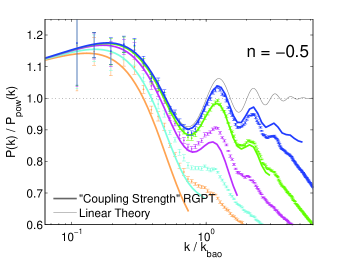
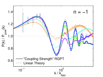
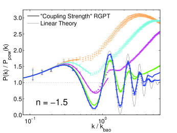
The primary PT results are presented in Fig. 11. At each output predictions are shown up to $k_{\rm{NL}}$, roughly the scales where these schemes are expected to break down. Generally, “coupling strength” RGPT and SPT/SPT+ give fair-to-good predictions for the non-linear damping of the wiggles (as discussed below, SPT+ uses the non-linear fitting functions in Appendix A for the powerlaw evolution). The good comparison with the simulations for the $n=-1.5$ case suggests that the non-linear shift can be adequately captured by PT. An exception to this is clearly the SPT+ predictions for the $n=-0.5$ case, which seem to significantly overpredict the damping of the BAO feature. We discuss the SPT/SPT+ predictions in more detail in the next section, breaking up the calculation into different “interaction” terms in an effort to gain insight into the non-linear physics. Predictions from “coupling strength” RGPT in Fig. 11 were not calculated by breaking up $P_{\rm{IC}}(k)$ in this way, since this scheme does a much better job than SPT in predicting the evolution of pure powerlaw spectra (Widrow et al., 2009).

Figure 11: A comparison of power spectrum results from Fig. 10 with quasi-linear predictions from standard perturbation theory (SPT/SPT+, dashed lines) and the “coupling strength” RGPT scheme (dot-dashed lines) from McDonald (2007). SPT+ treats the pure powerlaw evolution differently than SPT, using a fit to pure powerlaw simulation results (Appendix A) instead of the SPT prediction for the pure powerlaw evolution (Scoccimarro and Frieman, 1996). In each plot the $x$-axis limits are set to include the low $k$ measurements from simulations up to half the particle nyquist wavenumber, approximately the regime where the N-body results should be accurate.

V.4 SPT and SPT+

The 1-loop correction to the linear theory power spectrum is given by Makino et al. (1992)

$$P(k)=P_{L}(k)+P_{22}(k)+P_{13}(k)$$ (23)

where

$$\begin{array}[]{l l l}\displaystyle P_{22}(k)=&\displaystyle\frac{k^{3}}{98\left(2\pi\right)^{2}}\int_{0}^{\infty}drP_{L}\left(kr\right)\int_{-1}^{1}{dx}\,\times\\ &\displaystyle\,\,\ P_{L}\left[k\left(1+r^{2}-2rx\right)^{1/2}\right]\frac{\left(3r+7x-10rx^{2}\right)^{2}}{\left(1+r^{2}-2rx\right)^{2}}\end{array}$$ (24)

and

$$\begin{array}[]{l l l}\displaystyle P_{13}(k)=&\displaystyle\frac{k^{3}P_{L}(k)}{252\left(2\pi\right)^{2}}\int_{0}^{\infty}drP_{L}(kr)\Big{[}\frac{12}{r^{2}}-158+100r^{2}&\\ &\displaystyle\ \ -42r^{4}+\frac{3}{r^{3}}\left(r^{2}-1\right)^{3}(7r^{2}+2)\ln\bigg{|}\frac{1+r}{1-r}\bigg{|}\Big{]}.&\end{array}$$ (25)

Notice that in $P_{22}(k)$ and $P_{13}(k)$ the linear power spectrum appears twice, and as a result these terms increase in amplitude as the linear growth function to the fourth power.

For pure powerlaw spectra, by including UV and IR cutoffs and using sufficient care to avoid the singularity in the denominator of the kernel in $P_{22}(k)$, these integrals can be computed analytically (Scoccimarro and Frieman, 1996; Makino et al., 1992). In principle, it may also be possible to obtain an exact solution for 1-loop corrections to the analytic expression for $P_{\rm{IC}}(k)$ in Eq. 10, but the complexity of the $P_{22}(k)$ kernel is difficult to overcome or approximate.

To organize the calculation and for the most clarity in physical interpretation, we calculate the 1-loop corrections by treating separately the “interaction” terms that arise from inserting $P_{L}(k)=P_{\rm{pow}}(k)+P_{\rm{wig}}(k)$ (Eq. 4) in $P_{22}(k)$ and $P_{13}(k)$,

$$P_{22}(k)=\frac{k^{3}}{98(2\pi)^{2}}\bigg{[}\;\;\int{dr}P_{\rm{pow}}(kr)\int{dx}P_{\rm{pow}}\left[k(1+r^{2}-2rx)^{1/2}\right]f_{22}(r,x)$$

$$+\;2\int{dr}P_{\rm{pow}}(kr)\int{dx}P_{\rm{wig}}\left[k(1+r^{2}-2rx)^{1/2}\right]f_{22}(r,x)$$

$$+\int{dr}P_{\rm{wig}}(kr)\int{dx}P_{\rm{wig}}\left[k(1+r^{2}-2rx)^{1/2}\right]f_{22}(r,x)\;\bigg{]},$$ (26)

and likewise

$$P_{13}(k)=\frac{k^{3}}{252(2\pi)^{2}}\bigg{[}P_{\rm{pow}}(kr)\int{dr}P_{\rm{pow}}(kr)f_{13}(r)+P_{\rm{pow}}(kr)\int{dr}P_{\rm{wig}}(kr)f_{13}(r)$$

$$+\;P_{\rm{wig}}(kr)\int{dr}P_{\rm{pow}}(kr)f_{13}(r)+P_{\rm{wig}}(kr)\int{dr}P_{\rm{wig}}(kr)f_{13}(r)\bigg{]},$$ (27)

where $f_{22}(r,x)$ and $f_{13}(r)$ are short hand for the fully expressed kernels in Eqs. 24 and LABEL:eq:P13. For the terms where $P_{\rm{pow}}(k)$ appears twice – a.k.a. the powerlaw-powerlaw interactions – this result can be looked up in Scoccimarro and Frieman (1996) or computed using their approach. But since those results are often cutoff dependent and/or in poor agreement with simulations, we can potentially replace the powerlaw-powerlaw interactions and the linear theory powerlaw with a fitting function from pure powerlaw simulations, while still treating the remaining terms in $P_{22}(k)$ and $P_{13}(k)$ without any approximation. In Fig. 11 this approach is dubbed “SPT+” while “SPT” refers to treating the powerlaw-powerlaw interactions as in Scoccimarro and Frieman (1996). We discuss the remaining interaction terms in the next two sections.

Figure 12: Results for the powerlaw-wiggle interactions (cyan) and the wiggle-wiggle interactions (orange) for the three different powerlaw setups. Expectations from the diffusion model coupled with an analytic approximation for $P_{\rm{IC}}(k)$ in the $r_{0}/r_{\rm{bao}}\ll 1$ limit are shown for comparison in red. Positive corrections are shown in solid lines, negative corrections are shown in dashed lines. Note that for clarity the $n=-1.5$ plot is shown at the first output; the $n=-0.5$ and $-1$ plots are shown at the second output, which allows easier visual comparison with the linear theory power spectrum.

V.5 Powerlaw-Wiggle Interactions

Eqs. V.4 and 27 contain three terms that include both $P_{\rm{pow}}(k)$ and $P_{\rm{wig}}(k)$. Since these terms include dimensionless factors of $(r_{0}/r_{\rm{bao}})^{n+3}$, whereas in the remaining “wiggle-wiggle” interaction terms there appear factors of $(r_{0}/r_{\rm{bao}})^{2(n+3)}$, at fixed $r_{0}/r_{\rm{bao}}$ these powerlaw-wiggle interaction terms will generally give larger corrections to $P_{L}(k)$ than the “wiggle-wiggle” interactions, which are discussed in the next section. The powerlaw-wiggle terms were evaluated numerically to obtain the SPT and SPT+ results in Fig. 11. The $P_{13}(k)$ powerlaw-wiggle interactions are given by

$$\begin{array}[]{l l l}P_{13,\rm{pow}\textrm{-}\rm{wig}}(k)\;=&\\ \displaystyle\;\;\;\;\;\;\;\;\;\;\;\;\;\;\;\;\frac{k^{3}}{252(2\pi)^{2}}\bigg{[}P_{\rm{wig}}(kr)\int{dr}P_{\rm{pow}}(kr)f_{13}(r)&\\ \displaystyle\;\;\;\;\;\;\;\;\;\;\;\;\;\;\;\;\;\;\;\;\;\;\;\;\;\;\;\;\;\;\;+\;P_{\rm{pow}}(kr)\int{dr}P_{\rm{wig}}(kr)f_{13}(r)\bigg{]}.&\end{array}$$ (28)

For the second term in Eq. LABEL:eq:p13powwig, since $P_{\rm{wig}}(k)$ is exponentially damped at high $k$ and $P_{\rm{wig}}(k)\rightarrow$ constant for $k\rightarrow 0$, the result is cutoff independent. By using an approximation to the $P_{13}(k)$ kernel one can obtain a remarkably accurate approximate solution for this expression, which will be explained in the section on “wiggle-wiggle” interactions where this integral also appears.

The integral in the first term in Eq. LABEL:eq:p13powwig also appears in the calculations of Scoccimarro and Frieman (1996) for a variety of powerlaws. In this case IR divergences might be expected to be problematic, but, as explained by Makino et al. (1992), for steep powerlaws the IR divergence cancels with a corresponding term in $P_{22}(k)$ (in the present context the powerlaw-wiggle term in Eq. V.4) yielding finite results for $n>-3$. Unfortunately, there are still UV divergences for the $n=-0.5$ and $-1.0$ cases. We integrate up to $k_{\rm{max}}/k_{\rm{bao}}\approx 160$ in the results presented here.

The last powerlaw-wiggle interaction term, as just mentioned, is the second term in Eq. V.4. This term has a factor of two in front of it because a symmetry in the $P_{22}(k)$ kernel implies that if $P_{\rm{pow}}(k)$ and $P_{\rm{wig}}(k)$ are interchanged the result of the integral remains the same. We use this property to cross check the numerical integration of this term. Although we were unable to find an approximate analytic solution for this term, we note that the $dx$ integral can be computed analytically using the approximation $P_{\rm{wig}}(k)\sim\sin(kr_{\rm{bao}})/k$ and with a substitution of variables. This approximation is valid for $k\ll\sigma_{\rm{bao}}^{-1}$, still a relatively wide and interesting range of $k$.

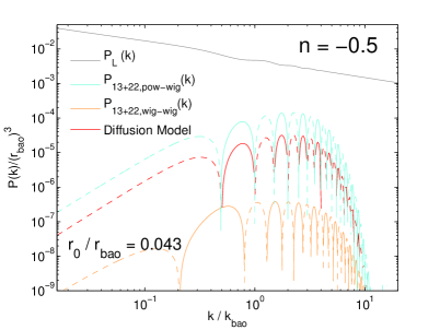
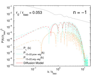
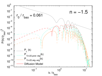
The results for the powerlaw-wiggle interactions are shown in cyan lines alongside the linear theory spectrum (gray solid lines) in Fig. 12. Also shown (in orange) are the wiggle-wiggle interactions discussed in the next section. A negative correction in this plot is shown with dashed lines, while positive corrections are shown with solid lines. Qualitatively, the results indicate that the powerlaw-wiggle interactions are approximately out of phase with linear theory and push and pull the wiggles in the right places to dampen out the BAO feature. A possible exception to this is the low $k$ correction for $n=-1.5$, but, in fact, the wide positive correction around $k/k_{\rm{bao}}\sim 0.5$ seems to explain the extra power seen on those scales in the simulation results (Fig. 10), which was not captured by the phenomenological model in Eq. 22.

For a more quantitative comparison to the powerlaw-wiggle results, Fig. 12 shows a model inspired by the diffusion behavior seen in the correlation function. If we suppose that the bump broadens out as in Eq. 15 and place this ansatz for $\sigma_{\rm{bao}}^{2}(r_{0})$ in the phenomenological model in Eq. 22, then in the limit where $r_{0}/r_{\rm{bao}}$ is small we expect the wiggles to evolve as

$$\begin{array}[]{l}P_{\rm{wig}}(k,r_{0})/r_{0}^{n+3}\sim\displaystyle e^{-k^{2}\sigma_{\rm{bao}}^{2}(r_{0})/2}\frac{\sin(kr_{\rm{bao}})}{k}\\ \;\;\;\displaystyle\approx e^{-k^{2}\sigma_{\rm{IC}}^{2}/2}\frac{\sin(kr_{\rm{bao}})}{k}\\ \;\;\;\;\;\;\;\;\;\displaystyle-k^{2}r_{\rm{bao}}^{2}\kappa_{n}\left(\frac{r_{0}}{r_{\rm{bao}}}\right)^{n+3}e^{-k^{2}\sigma_{\rm{IC}}^{2}/2}\frac{\sin(kr_{\rm{bao}})}{k}.\end{array}$$ (29)

Notice that since the linear theory wiggles grow in amplitude as the linear growth function squared (i.e. $r_{0}^{n+3}\sim Aa^{2}$ in Eq. 5), the extra factor of $r_{0}^{n+3}$ in Eq. 29 makes this correction grow as the linear growth function to the fourth power. This is the same dependence on the growth function as in SPT. We plot this expectation from the diffusion model – essentially $-k^{2}$ times the linear theory wiggles – alongside the powerlaw-wiggle results in Fig. 12. There are no free parameters to this comparison; $\kappa_{n}$ takes the same value as in § III.3, which gave a good fit to the correlation function results.

For the $n=-1$ and $-1.5$ cases the agreement with the diffusion model is quite good except for the caveat already mentioned with $n=-1.5$ for $k/k_{\rm{bao}}\sim 0.5$. For the $n=-0.5$ case, the shape of $P_{13+33,\rm{pow}\textrm{-}\rm{wig}}(k)$ agrees well with the diffusion model but the amplitude is about a factor of four larger. Fig. 12 suggests that the problem lies in the SPT+ prediction, which predicts too much damping of the BAO feature. (Increasing the high-$k$ cutoff would predict more damping.)

Comparing the diffusion model, which oscillates as $-\sin(kr_{\rm{bao}})$ in Fig. 12, to the powerlaw-wiggle interactions also reveals a slight phase difference between $P_{13+22,\rm{pow}\textrm{-}\rm{wig}}(k)$ and the diffusion model expectations. This is most easily visible for $n=-1.5$ in Fig. 12, which seems to oscillate as $-\sin(kr_{\rm{bao}}+\varphi)$ where $\varphi\approx 0.2$, while this phase is closer to $\varphi\approx 0.1$ for $n=-1$ and is consistent with zero for $n=-0.5$. This result implies that, in addition to damping the BAO feature, the powerlaw-wiggle interactions provide a shift, since a Taylor expansion of $\sin(kr_{\rm{bao}}/\alpha_{\rm{shift}})$ yields

$$\sin(kr_{\rm{bao}}/\alpha_{\rm{shift}})\approx\sin(kr_{\rm{bao}})-(\alpha_{\rm{shift}}-1)\cos(kr_{\rm{bao}})$$ (30)

and, without any approximation,

$$-\sin(kr_{\rm{bao}}-\varphi)=-\cos\varphi\,\sin(kr_{\rm{bao}})-\sin\varphi\,\cos(kr_{\rm{bao}}).$$ (31)

The last term on the right in Eq. 31 should provide the “push” to move the BAO feature to smaller scales, since $\sin\varphi\geq 0$ for the $\varphi$-values that match our results.

Figure 13: Highlighting the wiggle-wiggle interactions and showing, individually, $P_{13,\rm{wig}\textrm{-}\rm{wig}}(k)$ (red) and $P_{22,\rm{wig}\textrm{-}\rm{wig}}(k)$ (blue) which destructively interfere to produce the final result, $P_{13+22,\rm{wig}\textrm{-}\rm{wig}}(k)$ (cyan). Also shown for comparison are the linear-theory wiggles (Eq. 10) in black and a cosine function with a similar envelope and amplitude as $P_{13+22,\rm{wig}\textrm{-}\rm{wig}}(k)$. Note that the $y$-axis is normalized to be dimensionless and independent of powerlaw and epoch; see text for more details.

V.6 Wiggle-Wiggle Interactions

Though suppressed by a factor of $(r_{0}/r_{\rm{bao}})^{n+3}$ relative to the powerlaw-wiggle interactions, in Fig. 12 the wiggle-wiggle interactions are not completely negligible (at least for the $n=-1.5$ case), and by eye they appear about a half-period out of phase with the linear theory wiggles, just the kind of feature that gives rise to a shift of the BAO scale. We discuss these calculations in this section, with the convenience that because the functional form of $P_{\rm{wig}}(k)$ is independent of $n$, the wiggle-wiggle interactions are also independent of $n$ apart from the $(r_{0}/r_{\rm{bao}})^{2(n+3)}$ term out front. Since $P_{\rm{wig}}(k)\rightarrow$ constant at low $k$ and $P_{\rm{wig}}(k)$ decays rapidly to zero at high $k$, the integrals should be cutoff independent.

The task, then, is to evaluate the two remaining terms in Eqs. V.4 and 27. We treat both terms numerically, but, fortuitously, a remarkably accurate solution can be obtained for $P_{13,\rm{wig}\textrm{-}\rm{wig}}(k)$. Using $P_{\rm{wig}}(k)\sim\exp(-k^{2}\sigma_{\rm{bao}}^{2}/2)\sin(kr_{\rm{bao}})/k$, and by approximating the $P_{13}(k)$ kernel with $f_{13}(r)\approx-(352/5)\exp(-29r^{2}/11)-488/5$ one can show that

$$\int_{0}^{\infty}{dr}P_{\rm{wig}}(kr)f_{13}(r)\approx\;\;\;\;\;\;\;\;\;\;\;\;\;\;\;\;\;\;\;\;\;\;\;\;\;\;\;\;\;\;\;\;\;\;\;\;\;\;\;\;\;\;\;\;\;\;\;\;\;\;\;$$ (32)

$$-\frac{176\,\pi}{5\,k}\rm{Erf}\left(\frac{\sqrt{11}{\it k\,r_{\rm{bao}}}}{\sqrt{116+22{\it k^{2}\sigma_{\rm{bao}}^{2}}}}\right)-\frac{244\,\pi}{5\,k}\rm{Erf}\left(\frac{{\it r_{\rm{bao}}}}{\sqrt{2}{\it\sigma_{\rm{bao}}}}\right),$$

which is accurate to better than 8% for all $k$ and better than $1\%$ for $k/k_{\rm{bao}}\gtrsim 0.6$. The minus signs in this result imply that, when multiplied by $P_{\rm{wig}}(k)$ to obtain $P_{13,\rm{wig}\textrm{-}\rm{wig}}(k)$ as in Eq. 27, the result will oscillate like $-\sin(kr_{\rm{bao}})$.

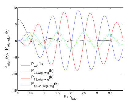
In Fig. 13, which shows the results for numerical integration of the wiggle-wiggle interactions, the $y$-axis has been normalized to be a dimensionless quantity that is independent of the powerlaw and epoch of interest, i.e.,

$$P_{\rm{wig},n}(k)\equiv\frac{P_{\rm{wig}}(k)}{r_{\rm{bao}}^{3}}\left(\frac{r_{\rm{bao}}}{r_{0}}\right)^{n+3}$$

$$P_{\rm{wig}\textrm{-}\rm{wig},n}(k)\equiv\frac{P_{\rm{wig}\textrm{-}\rm{wig}}(k)}{r_{\rm{bao}}^{3}}\left(\frac{r_{\rm{bao}}}{r_{0}}\right)^{2(n+3)}.$$

Clearly there is a great deal of destructive interference between $P_{13,\rm{wig}\textrm{-}\rm{wig}}(k)$ and $P_{22,\rm{wig}\textrm{-}\rm{wig}}(k)$ in Fig. 13. The sum of these terms, $P_{13+22,\rm{wig}\textrm{-}\rm{wig}}(k)$, which is of course much lower in amplitude than either $P_{13,\rm{wig}\textrm{-}\rm{wig}}(k)$ or $P_{22,\rm{wig}\textrm{-}\rm{wig}}(k)$, seems to oscillate at about a half-period out of phase with $P_{\rm{wig}}(k)$ as mentioned earlier. To highlight this we overplot with a green-dashed line a function proportional to $-\cos(kr_{\rm{bao}})$, which qualitatively follows the oscillations in $P_{13+22,\rm{wig}\textrm{-}\rm{wig}}(k)$ rather well. Since the $P_{22,\rm{wig}\textrm{-}\rm{wig}}(k)$ term seems to oscillate as $\sin(kr_{\rm{bao}}~{}-~{}\varphi)$ where $\varphi$ is small and positive, when added to $P_{13,\rm{wig}\textrm{-}\rm{wig}}(k)$, which oscillates as $-\sin(kr_{\rm{bao}})$ and with a similar envelope, these waves interfere as

$$\begin{array}[]{l l}\displaystyle-\sin(kr_{\rm{bao}})&+\;\;\sin(kr_{\rm{bao}}-\varphi)\\ &=\sin(kr_{\rm{bao}})(-1+\cos\varphi)-\sin\varphi\cos(kr_{\rm{bao}})\\ &\approx-\sin\varphi\,\cos(kr_{\rm{bao}}).\\ \end{array}$$ (33)

The green-dashed line, more specifically, shows this $-\cos(kr_{\rm{bao}})$ term multiplied by the analytically-derived envelope for $P_{13,\rm{wig}\textrm{-}\rm{wig}}(k)$ (i.e. Eq. 32 with appropriate constants and factors of $k$ and including a factor of $\exp(-k^{2}\sigma_{\rm{bao}}^{2}/2)$ from $P_{\rm{pow}}(k)$) and divided by a factor of four (i.e. $\sin\varphi\approx 1/4$) to approximately match the amplitude of $P_{13+22,\rm{wig}\textrm{-}\rm{wig}}(k)$. This model is only approximate – for example, there seems to be some weak $k$-dependence of the phase $\varphi$ in $P_{22,\rm{wig}\textrm{-}\rm{wig}}(k)$ – but, qualitatively, something like this phenomenological description must be going on.

This raises the question of whether, in SPT, the shift in the BAO scale comes primarily from the phase lag in the powerlaw-wiggle interactions or from $P_{13+22,\rm{wig}\textrm{-}\rm{wig}}(k)$. The answer, at least for $n=-1.5$ where the BAO scale moves significantly, is that the shift is similar in magnitude from both terms, and that both “push” the BAO scale in the same direction. Qualitatively, the same can be said for the $n=-1$ case, but the phase lag in the powerlaw-wiggle interactions is smaller and the $(r_{0}/r_{\rm{bao}})^{(n+3)}$-suppressed amplitude of wiggle-wiggle interactions is smaller still, so much less of a shift is expected. And in the $n=-0.5$ case there does not seem to be a phase lag in the powerlaw-wiggle interactions, while the wiggle-wiggle interactions are even more attenuated.

Figure 14: The results from fourier transforming the power spectrum predictions of “coupling strength” RGPT (Fig. 11) into correlation functions (dot dashed lines), compared with the results from simulations (points). The fourier transform was performed with a small amount of damping in order to suppress noise and the influence of the power spectrum for $k\gg k_{\rm{NL}}$, well beyond the regime where $P(k)$ predictions are expected to be reliable.

V.7 PT Results in Real Space

Returning to the “coupling strength” RGPT scheme, which is closely related to SPT, we show the results from integrating the $P(k)$ predictions from this scheme into two-point correlation functions in Fig. 14. Note that some of the outputs for the $n=-0.5$ case are omitted for clarity. At each output we apply a minimal damping to the power spectra to suppress noise and the influence of $P(k)$ for $k\gg k_{\rm{NL}}$ in the final result. Some PT schemes naturally include exponential damping in the predicted $P_{\rm{QL}}(k)$ (e.g. Matsubara, 2008), which is advantageous for computing $\xi(r)$ from PT. “Coupling strength” RGPT (and SPT) do not naturally include these factors, so the results for $\xi(r)$ may not be as clean-looking as other schemes, even though the $P(k)$ predictions may be quite reasonable. In SPT, for example, the $P(k)$ predictions for $k\gtrsim k_{\rm{NL}}$ with our setups are often large and inaccurate or predict $P(k)<0$ at some $k$. Therefore we do not show $\xi(r)$ predictions from SPT, which offer little insight in judging the accuracy of the scheme or in confirming the picture of how the BAO feature evolves as sketched out in the previous two sections.

With that disclaimer, the “coupling strength” RGPT predictions do a good job of rendering the evolution of the BAO feature in configuration space (Fig. 14). In all cases the broadening and attenuation of the bump are qualitatively accounted for, including the $n=-0.5$ case that was problematic in SPT; the success of the scheme in this case may even help explain why the area of the bump is not as precisely conserved as in the other setups (Fig. 5). And although it is difficult to see the trend (inferring $\xi(r)$ from $P(k)$ over a finite $k$ range, as described above, causes oscillations even when $P(k)$ is predicted perfectly), in the $n=-1.5$ case the scheme does seem to accurately predict the shift in the BAO peak. With the close correspondence between “coupling strength” RGPT and SPT, broadly speaking we interpret the success of “coupling strength” RGPT in Figs. 11 and 14 and the typically sensible results for SPT discussed in the previous two sections to imply that perturbation theory can accurately capture the non-linear evolution of the BAO feature with our class of initial conditions.

VI Discussion and comparison with $\Lambda$CDM

VI.1 $\Lambda$CDM-like Simulations

Figure 15: Left panel: The matter two-point correlation function results from four simulations using a canonical $\Lambda$CDM linear-theory power spectrum but evolving the initial conditions using $\Omega_{m}=1,\,\Omega_{\Lambda}=0$. The correlation function is shown at different epochs (points with error bars; solid when $\xi(r)>0$, circles when $\xi(r)<0$) with the linear theory correlation function overplotted (solid colored lines). The vertical dotted line shows the initial mean interparticle spacing. Center panel: The correlation function near the BAO scale. Vertical dotted lines show the expected shift from Seo et al. (2010) colored according to epoch. Also shown is the smooth $\xi_{\rm{nw}}(r)$ (black dot-dashed line) derived by fourier transforming $P_{\rm{nw}}(k)$ from Eisenstein and Hu (1998). Right panel: The result of subtracting $\xi_{\rm{nw}}(r)$ from the $\xi(r)$ measurements.

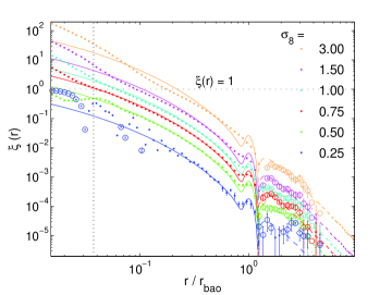
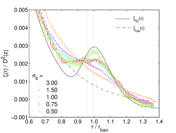
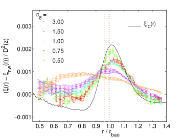
Having described and explained the non-linear evolution of the BAO-feature with our powerlaw setup in some detail, it is worth discussing the relevance of these results to the canonical $\Lambda$CDM cosmology. We approach this task first by simply assessing the resemblance of our results to $\Lambda$CDM. To aid in this comparison we performed a set of four simulations with an initial $\Lambda$CDM spectrum ($\Omega_{m}=0.226,\,\Omega_{\Lambda}=0.774$) as in Fig. 2 but evolved with $\Omega_{m}=1,\,\Omega_{\Lambda}=0$ so that $\sigma_{8}$ and $r_{0}/r_{\rm{bao}}$ in this case can avoid the freeze out limit and reach values comparable to the powerlaw setup. The $\Lambda$CDM-like simulations presented here were performed with essentially identical parameters as the earlier fiducial simulations in terms of box size, force resolution and number of particles. We show the primary $\xi(r)$ results in Fig. 15; the $r_{0}/r_{\rm{bao}}$ values for each output is shown in Table 2.

Table 2: $\Lambda$CDM outputs

	$r_{0}/r_{\rm{bao}}$	$\sigma_{8}$
	0.003	0.25
	0.019	0.5
	0.040	0.75
	0.062	1.0
	0.106	1.5
	0.218	3.0

Fig. 15 is fairly unremarkable except that it shows the non-linear evolution of the correlation function in $\Lambda$CDM well past $z=0$ and beyond the freeze out limit ($\sigma_{8}\sim 1.3$). As in Fig. 1, the overall amplitude of the BAO feature at fixed $r_{0}/r_{\rm{bao}}$ is more similar to the $n=-0.5$ case than to the cases with more large scale power. The models for the non-linear shift from Seo et al. (2010), shown with vertical dotted lines in the center and right panels of Fig. 1, predict shifts of $3-4$ % when extrapolated to the final output. The center panel also shows the smooth $\xi_{\rm{nw}}(r)$ correlation function, computed from a fourier transform of $P_{\rm{nw}}(k)$ from Eisenstein and Hu (1998), and in the right panel $\xi_{\rm{nw}}(r)$ is subtracted from the simulation data. In the center panel the combination of strong damping of the BAO feature and noise in the $\xi(r)$ measurement make any shift non-discernible. In the right panel the result of subtracting out $\xi_{\rm{nw}}(r)$ does visually resemble an attenuating gaussian (much more than $\xi(r)/\xi_{\rm{nw}}(r)$, which is not shown), but it is unclear whether the apparent drift of the BAO peak towards smaller scales, especially by the last output, is truly from the non-linear shift or whether the effect is simply from the changing broadband shape of $\xi(r)$. A plot of $(\xi(r)-\xi_{\rm{pow}}(r))/D^{2}(z)$ versus $r$ from any of our fiducial simulations would show a similar trend.

VI.2 Perturbation Theory and Modeling

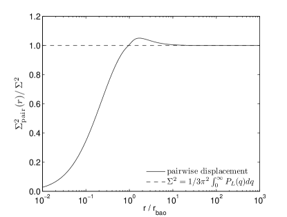
In§ V.2 we showed that a phenomenological approach matched the results from our fiducial simulations rather well. Eq. 22 bears a close resemblance to the damped-exponential models often used in the literature (e.g. Eisenstein et al., 2007; Seo et al., 2008), and we emphasize our conclusion that the broadening (damping) of the bump (wiggles) depends on the pairwise dispersion, $\Sigma_{\rm{pair}}^{2}$, rather than the rms displacement, $\Sigma^{2}$, which is sensitive to bulk motions. In Fig. 16, we compare $\Sigma_{\rm{pair}}^{2}/\Sigma^{2}$ on a wide range of scales for a $\Lambda$CDM spectrum (Fig. 2). Although we expect the two formulae to converge to the same result as $r\rightarrow\infty$, it is nevertheless surprising that $\Sigma_{\rm{pair}}^{2}(r_{\rm{bao}})$ differs by less than 2% from the $\Sigma^{2}$ displacement. In the literature some groups use Eq. 2 to predict the damping, while for others $\Sigma^{2}$ is a free parameter that is fit to simulations (e.g. Seo et al., 2008). In our view, like that of Eisenstein et al. (2007), it is $\Sigma_{\rm{pair}}^{2}(r_{\rm{bao}})$ that matters physically, and the success of models based on Eq. 2 is a lucky coincidence that holds in $\Lambda$CDM-like models but can fail, by an infinite factor, for powerlaw models.

Figure 16: The rms pairwise displacement (Eq. 11; solid) at different scales using $\Lambda$CDM initial conditions divided by the commonly used rms displacement formula (Eq. 2; dashed), which includes the contribution from bulk motions. Both quantities scale as the linear growth function squared, so the result shown is independent of epoch.

Another widely-used phenomenological approach assumes a model for $P_{\rm{NL}}(k)$ motivated by Renormalized Perturbation Theory (RPT; Crocce and Scoccimarro, 2006). In these models the non-linear shift comes directly from including $P_{22}(k)$ in the phenomenological form, or, in real space, from modeling the shift with the closely-related $\xi_{\rm{mc}}(r)$ ansatz and calibrating the amplitude of this term to N-body results (e.g. Sánchez et al. (2008); Montesano et al. (2010); Crocce et al. (2011)). Using our setup and a natural value for the amplitude of this term, in § III.4 we showed that this approach adequately captures the shift in real space for the first output of the $n=-1.5$ case (when $\sigma_{8}=0.5$). By the second output (corresponding to $\sigma_{8}=1$), however, it fails, and although not rigorously justified by the derivation of the term, we argue that the formula would more accurately predict the shift if the broadening of the bump could be incorporated into $\xi_{\rm{mc}}(r)$. This may have been previously unnoticed because the shift in $\Lambda$CDM when $\sigma_{8}\sim 1$ is smaller than the shift in the $n=-1.5$ case, and the amplitude of the bump, i.e., $\xi(r_{\rm{bao}})$, is significantly smaller in $\Lambda$CDM than in the $n=-1.5$ setup.

Finally, the success of the “coupling strength” RGPT method (McDonald, 2007) in matching our simulation results, both in fourier space and in real space, may certainly be informative to ongoing efforts to model the BAO evolution with ab initio predictions from PT. Carlson et al. (2009) show that this scheme also does a reasonable job in predicting the non-linear power spectra of $\Lambda$CDM and cCDM cosmologies. Except for SPT Makino et al. (1992) we ignored other PT schemes, but in principle the predictions from many other PT schemes could be compared to our simulation results and useful insights gained from the kind of comparisons presented in § V.3. This would no doubt be useful for BAO studies, and, more broadly, Valageas and Nishimichi (2011) find that the largest deficiency of the halo model is in capturing the transition from the 1-halo to 2-halo term, precisely the scales where the perturbation theory predictions are most important.

VII Summary

Motivated by the importance of accurate modeling of the BAO feature in large scale structure for interpreting the results of future dark energy experiments, we have used N-body simulations to investigate the evolution of a BAO-like feature in a simpler, alternative setting, where it modulates an underlying powerlaw initial power spectrum in an $\Omega_{m}=1$ universe. Specifically, our initial conditions have the correlation function defined by Eq. 1, with a gaussian multiplicative bump centered at scale $r_{\rm{bao}}$ and the amplitude $A_{\rm{bump}}$ and width $\sigma_{\rm{bao}}$ chosen in approximate agreement with $\Lambda$CDM expectations. The corresponding initial power spectrum follows Eq. 10 to an excellent approximation. For given values of $A_{\rm{bump}}$, $\sigma_{\rm{bao}}$, and the powerlaw spectral index $n$, non-linear matter clustering statistics (including the correlation function and power spectrum) should depend only on the ratio $r_{0}/r_{\rm{bao}}$, where $r_{0}$ is the correlation length defined by $\xi(r_{0})=1$. We evolve our simulations to values of $r_{0}/r_{\rm{bao}}$ much higher than traditional $\Lambda$CDM models, with final outputs corresponding to $\sigma_{8}=4.0\,(n=-1.5)$, $6.0\,(n=-1)$, and $12.0\,(n=-0.5)$ if we define a physical scale by setting $r_{\rm{bao}}=100h^{-1}$Mpc. Our standard simulations have box side $L_{\rm{box}}/r_{\rm{bao}}=20$ and $512^{3}$ particles. We use our simulations to develop physical intuition for BAO evolution and to test analytic descriptions in a regime far from that where they have been tested previously. In this respect, the spirit of our exercise is similar to the cCDM investigation of Carlson et al. (2009) and Padmanabhan and White (2009).

Consistent with $\Lambda$CDM studies, we find that the strongest effect of non-linear evolution on the BAO feature in $\xi(r)$ is to flatten and broaden the bump, with $A_{\rm{bump}}$ decreasing and $\sigma_{\rm{bao}}$ increasing. To a good approximation, failing only at late times in the $n=-0.5$ model, the area of the gaussian bump, proportional to $A_{\rm{bump}}\times\sigma_{\rm{bao}}$, remains constant, which suggests that pairs are “diffusing” out of the shell corresponding to the initial BAO feature (see the physical description of Eisenstein et al. (2007)). The evolution of the bump width is well described by a model in which the non-linear $\sigma_{\rm{bao}}$ is the quadrature sum of the initial width and a length proportional to $\Sigma_{\rm{pair}}$, the rms relative displacement (computed from linear theory) of pairs separated by $r=r_{\rm{bao}}$. The constant of proportionality varies with $n$, but the same constant that describes our standard $n=-1$ model also describes the faster evolution of an $n=-1$ model with a “skinny” initial bump, supporting the validity of the diffusion interpretation. For $n=-1.5$ (where the relevant integral converges without a small scale UV cutoff) the diffusion constant computed ab initio describes the bump evolution accurately. We emphasize that it is $\Sigma_{\rm{pair}}$ rather than the rms absolute displacement $\Sigma$ that is relevant to analytic descriptions of our models. The latter quantity has an infrared divergence for $n\leq-1$, but this divergence corresponds to bulk translations induced by very large scale modes, which cannot affect the BAO peak itself. We think that the appearance of $\Sigma$ rather than $\Sigma_{\rm{pair}}$ in many analytic models of BAO evolution is at best an approximation restricted to CDM-like models with a turnover in $P(k)$; by coincidence, $\Sigma\approx\Sigma_{\rm{pair}}(r_{\rm{bao}})$ for $\Lambda$CDM.

The location of the BAO peak, defined by the scale $r_{\rm{peak}}$ of a gaussian fit to the non-linear $\xi(r)$ divided by the linear theory powerlaw, stays constant within the statistical precision of our measurements for the $n=-0.5$ and $n=-1$ models, even when these are evolved to a highly non-linear stage where the bump amplitude has dropped by a factor of $\sim 4-10$ from its initial value. For $n=-1.5$, on the other hand, the peak location shifts to smaller $r$, an effect that is already noticeable at the first output ($r_{0}/r_{\rm{bao}}=0.024$, equivalent to $\sigma_{8}=0.5$) and that grows to a 30% drop by $r_{0}/r_{\rm{bao}}=0.386$ (equivalent to $\sigma_{8}=4.0$). The analytic models of Smith et al. (2008) and Crocce and Scoccimarro (2008) accurately predict that shifts should be much larger for $n=-1.5$ than for $n=-0.5$ and $n=-1$, and the Smith et al. (2008) model accurately describes the evolution of the peak location for $n=-1.5$. However, both models predict non-linear shifts in the $n=-0.5$ and $n=-1$ cases that are inconsistent with our simulation results at late times.

We carried out a number of additional numerical tests varying either numerical parameters or the physical model. Our fiducial simulations have $L_{\rm{box}}/r_{\rm{bao}}=20$ and an initial mean interparticle spacing smaller than $r_{\rm{bao}}$ by a factor of $r_{\rm{bao}}/n_{p}^{-1/3}=25$. We found consistent results in simulations with $L_{\rm{box}}/r_{\rm{bao}}=10$ and $r_{\rm{bao}}/n_{p}^{-1/3}=50$, indicating that a box size ten times the BAO scale is acceptable. We found marginal discrepancies for $256^{3}$ simulations with $r_{\rm{bao}}/n_{p}^{-1/3}=12.5$. Success of the box size test and other internal consistency tests is achieved only because we include the integral constraint corrections described in Appendix B, which make a noticeable difference for $n=-1$ and an important difference for $n=-1.5$. In other tests, we show that BAO evolution is nearly identical in an $\Omega_{m}=1$ model and a model with $\Omega_{m}=0.3$, $\Omega_{\Lambda}=0.7$ (and the same initial conditions) provided they are evaluated at the same value of $r_{0}/r_{\rm{bao}}$ (or, equivalently, the same value of the linear growth function).

For more thorough tests of analytic models, we turned to a fourier space description using the non-linear matter power spectrum. A “phenomenological” model in which we combine numerical results for the non-linear power spectrum of a pure powerlaw model (Appendix A and references therein) with our gaussian fits to the evolution of the BAO bump in $\xi(r)$ gives a remarkably accurate description of the full non-linear outputs of the $n=-1$ and $n=-1.5$ models. This model assumes no shift of the $\xi(r)$ peak location for $n=-0.5$ and $n=-1$ and $r_{\rm{peak}}/r_{\rm{bao}}=1-1.08(r_{0}/r_{\rm{bao}})^{1.5}$ for $n=-1.5$. The success of this model suggests that the BAO bump has little effect on the non-linear evolution of the underlying “smooth” power spectrum. At least for $r_{0}/r_{\rm{bao}}<0.2$, we expect that this model is a more accurate description than our numerical $P(k)$ measurements themselves, since it draws on self-similar scaling results from pure powerlaw spectra that have wider dynamic range than our simulations.

We compared our results to predictions of two ab initio analytic approaches, “standard” 1-loop perturbation theory (SPT; e.g. Vishniac (1983); Makino et al. (1992)) and the “coupling strength” RGPT scheme of McDonald (2007). This scheme provides a quite accurate description of the low-$k$ evolution in all cases, including $n=-1.5$ where the peak location shifts significantly, and it produces good but not perfect agreement with the evolution of the $\xi(r)$ bump in configuration space. For SPT, we break up the terms into distinct “interactions” between the powerlaw and “wiggle” components of the linear power spectrum, both to obtain physical insight and to allow us to define a more accurate “SPT+” scheme that uses numerical results for pure powerlaw evolution and perturbation theory to describe the interaction terms that involve the “wiggle” spectrum. SPT alone gives a reasonable description of the early $P(k)$ outputs for $n=-1.5$, but on the whole “coupling strength” RGPT is substantially more accurate and has a wider range of validity.

The high statistical precision achievable with future BAO surveys — with $\sim 0.2\%$ cosmic variance distance scale errors for $z\geq 1$ and redshift bins $\Delta z\approx 0.2$ (Seo and Eisenstein, 2007) — puts stringent demands on theoretical models. Exploiting the power of these surveys will require large numerical simulations supplemented by the physical insight and modeling flexibility afforded by analytic methods. The simulation results presented here offer valuable “stress tests” of numerical and analytic approaches in regimes beyond those where they are usually applied, and they allow isolation of distinct physical effects. Two natural directions that we plan to explore in future work are the clustering of biased tracers — in particular the massive halos expected to host luminous galaxies — and the impact of redshift-space distortions on BAO measurement from galaxy clustering. We will also investigate the impact of the initial conditions algorithms, comparing the scheme advocated by Sirko (2005) for simulation ensembles to the traditional scheme of mean density boxes used here. The combination of future BAO surveys and improved theoretical models will lead, ultimately, to new insights on the energy and matter contents of the cosmos.

Appendix A Results from Pure Powerlaw Simulations

Having performed pure powerlaw simulations for the sake of better understanding the non-linear power spectra of our fiducial simulations, we give fitting functions for the $n=-0.5,-1$ and $-1.5$ powerlaws using $512^{3}$-particle Gadget2 simulations, which were set up similarly to the fiducial simulations as outlined in § II. The interested reader can consult the excellent paper by Widrow et al. (2009) to find fitting functions for other powerlaws.

Fig. 17 shows our primary powerlaw results compared against other fitting functions in the literature, either specific to each powerlaw or universal fitting functions designed to match a variety of powerlaws and cosmologies. Our simulations do not extend to impressively large values of $k/k_{\rm{NL}}$ compared to Widrow et al. (2009), in part because of how long we chose to evolve the simulations and in part because we chose, conservatively, to only show $k$-values up to one fourth the particle nyquist wavenumber, i.e., half the rule of thumb recommended by Heitmann et al. (2010). However, we run a number of realizations of each powerlaw (six realizations for $n=-0.5$, four for $n=-1$, and ten for $n=-1.5$), which is a few to many more than in previous studies. As a result the error bars in Fig. 17, which show the measured errors on the mean from all realizations in each case, can be quite constraining.

Figure 17: Results from pure powerlaw simulations (colored points with error bars) compared to various fitting functions in the literature (black dotted, dash-dotted or dashed lines). Also shown is our improved fit in thick black lines (Eqs. 34 & 35) and, for $n=-1.5$, the analytically derived SPT prediction from Appendix B of Scoccimarro and Frieman (1996) is shown with a thick black dashed line. For the Smith et al. (2003) functions in the $n=-1$ and $n=-1.5$ panels, we use modified formulas that correct typographical errors in the original paper (see eq. 36 and following text).

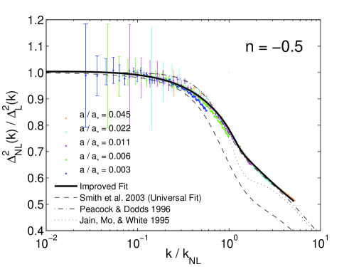
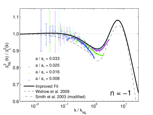
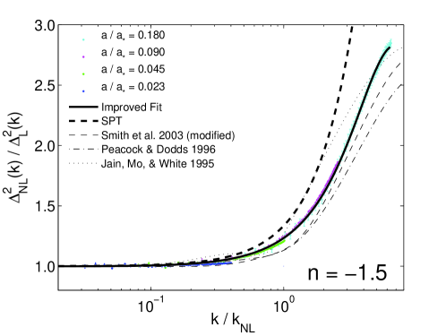
Since there is always a concern that the numerical results will be invalidated when the clustering power on the scale of the box becomes large, following the convention of Widrow et al. (2009) we show the value of $a/a_{*}=(k_{\rm{B}}/k_{\rm{NL}})^{(n+3)/2}$ for each output in all three panels as an indicator for how close the non-linear scale has come to the scale of the box. As stated previously, even our simulations with the most large scale clustering ($n=-1.5$) fall comfortably below the threshold where the loss of clustering power from beyond the box scale might be a concern. More quantitatively, in Fig. 17, $a/a_{*}$ is typically $\ll 1$, and in the $n=-1.5$ case the last output only reaches $a/a_{*}=0.18$. Importantly, the later outputs seem to show the self-similar scaling required by the scale-free nature of the initial conditions, the results falling along the same curve when plotted against $k/k_{\rm{NL}}$ and divided by $\Delta_{L}^{2}(k)$. For the earlier outputs this scaling seems not to have set in yet in some cases, a fact revealed by the self-similar test. Therefore we define the non-linear fitting functions as much as possible to the later outputs which are least affected by the clustering signature of the initial grid.

We present our non-linear fitting functions as a generalization of the functional form in Widrow et al. (2009):

$$\Delta_{\rm{NL}}^{2}(k)=\Delta_{\rm{L}}^{2}(k)f_{n}(k/k_{\rm{NL}}),$$ (34)

$$f_{n}(x)=\left(\frac{1+Ax+Bx^{\alpha}+Ex^{\epsilon}}{1+Cx^{\gamma}+Dx^{\delta}}\right)^{\beta}.$$ (35)

Table 3: Best-fit Parameters for the Non-linear Fitting Function

$$\begin{array}[]{ccccccccccc}n&A&B&C&D&E&\alpha&\beta&\gamma&\delta&\epsilon\\ -0.5&-0.1309&0.1131&0.1296&-0.02472&0.0&8.599&2.066&8.714&0.4565&0.0\\ -1&-0.4722&0.3542&0.04449&-0.2020&-0.08956&1.358&1.447&1.911&0.3963&0.2564\\ -1.5&-0.0792&0.1704&0.008748&0.0&0.0&1.225&2.672&2.1306&0.0&0.0\end{array}$$

Our $n=-1$ results primarily drive the necessity of making this generalization. The $n=-1.5$ results seem reasonably well represented with the Widrow formula, so we set $E=D=\epsilon=\delta=0$ in that case, while in the $n=-0.5$ case we set $E=\epsilon=0$, which still allows sufficient degrees of freedom to adequately describe the simulation results. The fitting formula above should be accurate to $k/k_{\rm{NL}}\sim 5$ for $n=-0.5$, $k/k_{\rm{NL}}\sim 100$ for $n=-1$ (larger because the fit was forced to closely match the results of Widrow et al. (2009) at high $k$), and $k/k_{\rm{NL}}\sim 6.5$ for $n=-1.5$.

A.1 Specific Comments on n = -0.5, -1, & -1.5

To our knowledge the most recent work to explicitly show the non-linear evolution of a pure $n=-0.5$ spectrum from simulations is Jain et al. (1995), whose universal fitting function we plot alongside our results in Fig. 17. The universal fitting functions of Peacock and Dodds (1996) and Smith et al. (2003) are capable of making predictions for $n=-0.5$, but their fitting functions were trained only on $n=0$ and $n=-1$ simulations to set the scaling in this regime. With this caveat the remarkable agreement of the prediction of Peacock and Dodds (1996) and our $n=-0.5$ results seems somewhat fortuitous and the disagreement with the Smith et al. (2003) prediction seems not so surprising.

The discrepancy between our $n=-1$ simulation results and the Widrow fitting function is entirely explainable by the sparseness of their measurements in the quasi-linear regime and is not indicative of any kind of problem with either their or our simulations. At larger $k/k_{\rm{NL}}$ both results overlap nicely, and we define our fitting function to closely match theirs for $k/k_{\rm{NL}}\gtrsim 3$. Also plotted alongside the $n=-1$ simulation results is a fitting function specific to $n=-1$ from Appendix B of Smith et al. (2003). There is a typo in their fitting formula (their Eq. B1), which should read

$$f_{EdS}(y)=y\left[\frac{1+y/a+(y/b)^{2}+(y/c)^{\alpha-1}}{(1+(y/d)^{(\alpha-\beta)\gamma})^{1/\gamma}}\right]$$ (36)

(R. Smith private communication). The corrected formula for $n=-1$ is shown in the middle panel of Fig. 17, and although at $k\sim k_{\rm{NL}}$ it deviates strongly from either fitting function, at lower $k$ it matches our results reasonably well.

Appendix B of Smith et al. (2003) also includes a set of constants tuned specifically for their $n=-1.5$ results, but there is a typo in their table in the reported value of $\alpha$. From quantitative comparison to their Fig. 11 (especially at large $k/k_{\rm{NL}}$), the correct value seems to be $\alpha\approx 7$, rather than $\alpha=0.707$ as reported. We show this result alongside our other results for $n=-1.5$ in the right panel of Fig. 17. Since both Peacock and Dodds (1996) and Jain et al. (1995) include $n=-1.5$ simulations in their universal fits, we also show the predictions of their fitting functions. Finally, we plot the expectations from SPT for $n=-1.5$ in the limit that the UV cutoff goes to infinity, as in Appendix B of Scoccimarro and Frieman (1996). In our fiducial simulations this is the formula used to predict the evolution of the powerlaw in the SPT model shown in Fig. 11. The SPT+ models in Fig. 11 instead use the non-linear fitting functions just described to model the evolution of the $n=-0.5$ and $n=-1$ powerlaws.

Appendix B Integral-Constraint Corrections to the Measured Matter Autocorrelation Function

When estimating the correlation function in our simulations, we divide the average number of neighbors found around particles in the separation range $r\rightarrow r+dr$ by the number expected for an unclustered distribution of number density $N/V$:

$$\hat{\xi}(r)={\langle N_{\rm nbr}(r\rightarrow r+dr)\rangle\over 4\pi r^{2}\,dr\times N/V}-1~{},$$ (37)

where $V$ is the simulation box volume, $N$ is the total number of particles, and we use $\hat{\xi}(r)$ to distinguish this estimated correlation function from the true correlation function $\xi_{\rm true}(r)$ of the underlying cosmological model. This procedure is subject to a well known “integral constraint” bias (described by, e.g., (Peebles, 1980, §47)), which arises because the simulation volume itself is forced to have the cosmological mean density. The fact that the total number of particle pairs in the box is $N(N-1)/2\approx(1/2)N^{2}$ imposes the requirement

$$\int_{V_{\rm{box}}}d^{3}r\,\hat{\xi}(r)\approx\int_{0}^{R_{S}=L_{\rm{box}}/1.61}4\pi r^{2}\,dr\,\hat{\xi}(r)=0~{},$$ (38)

where we have approximated the integral over the box volume as the integral over a sphere of volume $(4\pi/3)R_{S}^{3}=V=L_{\rm{box}}^{3}$. For large volume $\Lambda$CDM simulations, the bias in $\hat{\xi}(r)$ is usually a small effect because the true correlation function goes rapidly to zero, then becomes negative at large $r$, making equation (38) easy to satisfy. However, for powerlaw models with negative $n$, the slow decay of the correlation function makes the integral constraint bias more important.

We account for the integral constraint by assuming that it produces a scale-independent additive bias, so that the mean value of $\hat{\xi}(r)$ averaged over an ensemble of simulations would be

$$\hat{\xi}(r)=\xi_{\rm true}(r)+\xi_{\rm bias}~{}.$$ (39)

For our powerlaw models, Eq. (38) then implies

$$\int_{0}^{R_{S}}4\pi r^{2}\,dr\,\left[\xi_{\rm true}(r)+\xi_{\rm bias}\right]=0$$ (40)

and thus

$$\xi_{\rm bias}=-\,{3\over 4\pi R_{S}^{3}}\int_{0}^{R_{S}}4\pi r^{2}\,dr\,\xi_{\rm true}(r)={3\over n}\left({r_{0}\over R_{S}}\right)^{n+3}~{},$$ (41)

where we have used the linear theory $\xi_{L}(r)=(r/r_{0})^{-(n+3)}$ for $\xi_{\rm true}(r)$. More elegantly, this bias is simply the volume-averaged correlation function, $\xi_{\rm{bias}}=-\bar{\xi}_{L}(R_{s})$, which agrees with the conclusions of (Bernardeau et al., 2002, §6.4.2), who derived this term using the sophisticated error analysis in Landy and Szalay (1993).

In all our figures we plot the corrected correlation function

$$\xi(r)=\hat{\xi}(r)+\bar{\xi}_{L}(R_{S})~{}.$$ (42)

At large $r$, the fractional correction is

$${\xi(r)-\hat{\xi}(r)\over\xi_{L}(r)}={3\over-n}\left(1.61r\over L_{\rm{box}}\right)^{n+3}~{}.$$ (43)

Since $r$ is always less than $L_{\rm{box}}/1.61$, this correction is fractionally larger for more negative $n$ and, at fixed $n$, the effect is most important for $r$ approaching the box scale as previously mentioned. In practice, we find that the integral constraint makes little quantitative difference to the appearance of, e.g., Figs. 3 & 8 for $n=-0.5$, a noticeable difference for $n=-1$, and an important difference for $n=-1.5$. In particular, the box size convergence tests in Figure 8 succeed for $n=-1.5$ only because we include the integral constraint correction.

References

- McDonald (2007) P. McDonald, PRD 75, 043514 (2007).
- Eisenstein et al. (2005) D. J. Eisenstein, I. Zehavi, D. W. Hogg, R. Scoccimarro, M. R. Blanton, R. C. Nichol, R. Scranton, H. Seo, M. Tegmark, Z. Zheng, et al., ApJ 633, 560 (2005).
- Cole et al. (2005) S. Cole, W. J. Percival, J. A. Peacock, P. Norberg, C. M. Baugh, C. S. Frenk, I. Baldry, J. Bland-Hawthorn, T. Bridges, R. Cannon, et al., MNRAS 362, 505 (2005).
- Peebles and Yu (1970) P. J. E. Peebles and J. T. Yu, ApJ 162, 815 (1970).
- Eisenstein et al. (1998) D. J. Eisenstein, W. Hu, and M. Tegmark, ApJL 504, L57+ (1998).
- Blake and Glazebrook (2003) C. Blake and K. Glazebrook, ApJ 594, 665 (2003).
- Seo and Eisenstein (2003) H. Seo and D. J. Eisenstein, ApJ 598, 720 (2003).
- Percival et al. (2010) W. J. Percival, B. A. Reid, D. J. Eisenstein, N. A. Bahcall, T. Budavari, J. A. Frieman, M. Fukugita, J. E. Gunn, Ž. Ivezić, G. R. Knapp, et al., MNRAS 401, 2148 (2010).
- Kazin et al. (2010) E. A. Kazin, M. R. Blanton, R. Scoccimarro, C. K. McBride, A. A. Berlind, N. A. Bahcall, J. Brinkmann, P. Czarapata, J. A. Frieman, S. M. Kent, et al., ApJ 710, 1444 (2010).
- Drinkwater et al. (2010) M. J. Drinkwater, R. J. Jurek, C. Blake, D. Woods, K. A. Pimbblet, K. Glazebrook, R. Sharp, M. B. Pracy, S. Brough, M. Colless, et al., MNRAS 401, 1429 (2010).
- Blake et al. (2011) C. Blake, T. Davis, G. Poole, D. Parkinson, S. Brough, M. Colless, C. Contreras, W. Couch, S. Croom, M. J. Drinkwater, et al., eprint arXiv:1105.2862.
- Hill et al. (2008) G. J. Hill, K. Gebhardt, E. Komatsu, N. Drory, P. J. MacQueen, J. Adams, G. A. Blanc, R. Koehler, M. Rafal, M. M. Roth, et al., in Astronomical Society of the Pacific Conference Series, edited by T. Kodama, T. Yamada, & K. Aoki (2008), vol. 399, p. 115.
- Schlegel et al. (2009a) D. Schlegel, M. White, and D. Eisenstein, eprint arXiv:0902.4680.
- Kaiser et al. (2002) N. Kaiser, H. Aussel, B. E. Burke, H. Boesgaard, K. Chambers, M. R. Chun, J. N. Heasley, K. Hodapp, B. Hunt, R. Jedicke, et al., in Society of Photo-Optical Instrumentation Engineers (SPIE) Conference Series, edited by J. A. Tyson & S. Wolff (2002), vol. 4836, pp. 154–164.
- The Dark Energy Survey Collaboration (2005) The Dark Energy Survey Collaboration, eprint arXiv:astro-ph/0510346.
- LSST Science Collaboration (2009) LSST Science Collaboration, eprint arXiv:0912.0201.
- Schlegel et al. (2009b) D. J. Schlegel, C. Bebek, H. Heetderks, S. Ho, M. Lampton, M. Levi, N. Mostek, N. Padmanabhan, S. Perlmutter, N. Roe, et al., eprint arXiv:0904.0468.
- Blanford and the Committee for a Decadal Survey of Astronomy and Astrophysics (2010) R. D. Blanford and the Committee for a Decadal Survey of Astronomy and Astrophysics, New Worlds, New Horizons in Astronomy and Astrophysics (The National Academies Press, Washington, D.C, 2010).
- Laureijs et al. (2009) R. Laureijs et al., eprint arXiv:0912.0914.
- Carlson et al. (2009) J. Carlson, M. White, and N. Padmanabhan, PRD 80, 043531 (2009).
- Padmanabhan and White (2009) N. Padmanabhan and M. White, PRD 80, 063508 (2009).
- Eisenstein et al. (2007) D. J. Eisenstein, H. Seo, and M. White, ApJ 664, 660 (2007).
- Seo et al. (2008) H. Seo, E. R. Siegel, D. J. Eisenstein, and M. White, ApJ 686, 13 (2008).
- Seo et al. (2010) H. Seo, J. Eckel, D. J. Eisenstein, K. Mehta, M. Metchnik, N. Padmanabhan, P. Pinto, R. Takahashi, M. White, and X. Xu, ApJ 720, 1650 (2010).
- Smith et al. (2008) R. E. Smith, R. Scoccimarro, and R. K. Sheth, PRD 77, 043525 (2008).
- Takahashi et al. (2009) R. Takahashi, N. Yoshida, M. Takada, T. Matsubara, N. Sugiyama, I. Kayo, A. J. Nishizawa, T. Nishimichi, S. Saito, and A. Taruya, ApJ 700, 479 (2009).
- Crocce and Scoccimarro (2008) M. Crocce and R. Scoccimarro, PRD 77, 023533 (2008).
- Montesano et al. (2010) F. Montesano, A. G. Sánchez, and S. Phleps, MNRAS pp. 1223–+ (2010).
- Sánchez et al. (2008) A. G. Sánchez, C. M. Baugh, and R. Angulo, MNRAS 390, 1470 (2008).
- Efstathiou et al. (1988) G. Efstathiou, C. S. Frenk, S. D. M. White, and M. Davis, MNRAS 235, 715 (1988).
- Bertschinger and Gelb (1991) E. Bertschinger and J. M. Gelb, Computers in Physics 5, 164 (1991).
- Makino et al. (1992) N. Makino, M. Sasaki, and Y. Suto, PRD 46, 585 (1992).
- Lacey and Cole (1994) C. Lacey and S. Cole, MNRAS 271, 676 (1994).
- Colombi et al. (1996) S. Colombi, F. R. Bouchet, and L. Hernquist, ApJ 465, 14 (1996).
- Jain et al. (1995) B. Jain, H. J. Mo, and S. D. M. White, MNRAS 276, L25 (1995).
- Smith et al. (2003) R. E. Smith, J. A. Peacock, A. Jenkins, S. D. M. White, C. S. Frenk, F. R. Pearce, P. A. Thomas, G. Efstathiou, and H. M. P. Couchman, MNRAS 341, 1311 (2003).
- Widrow et al. (2009) L. M. Widrow, P. J. Elahi, R. J. Thacker, M. Richardson, and E. Scannapieco, MNRAS 397, 1275 (2009).
- Peebles (1980) P. J. E. Peebles, The large-scale structure of the universe (Princeton University Press, Princeton, 1980).
- Crocce et al. (2006) M. Crocce, S. Pueblas, and R. Scoccimarro, MNRAS 373, 369 (2006).
- Zel’Dovich (1970) Y. B. Zel’Dovich, A&A 5, 84 (1970).
- Lewis et al. (2000) A. Lewis, A. Challinor, and A. Lasenby, ApJ 538, 473 (2000).
- Komatsu et al. (2011) E. Komatsu, K. M. Smith, J. Dunkley, C. L. Bennett, B. Gold, G. Hinshaw, N. Jarosik, D. Larson, M. R. Nolta, L. Page, et al., ApJS 192, 18 (2011).
- Springel (2005) V. Springel, MNRAS 364, 1105 (2005).
- Barnes and Hut (1986) J. Barnes and P. Hut, Nature 324, 446 (1986).
- Crocce et al. (2011) M. Crocce, A. Cabré, and E. Gaztañaga, MNRAS 414, 329 (2011).
- Cohn (2006) J. D. Cohn, Nature 11, 226 (2006).
- Gurbatov et al. (1989) S. N. Gurbatov, A. I. Saichev, and S. F. Shandarin, MNRAS 236, 385 (1989).
- Weinberg and Gunn (1990) D. H. Weinberg and J. E. Gunn, MNRAS 247, 260 (1990).
- Zheng et al. (2002) Z. Zheng, J. L. Tinker, D. H. Weinberg, and A. A. Berlind, ApJ 575, 617 (2002).
- Nusser and Colberg (1998) A. Nusser and J. M. Colberg, MNRAS 294, 457 (1998).
- Hockney and Eastwood (1981) R. W. Hockney and J. W. Eastwood, Computer Simulation Using Particles (McGraw-Hill, New York, 1981).
- Heitmann et al. (2010) K. Heitmann, M. White, C. Wagner, S. Habib, and D. Higdon, ApJ 715, 104 (2010).
- Jing (2005) Y. P. Jing, ApJ 620, 559 (2005).
- Colombi et al. (2009) S. Colombi, A. Jaffe, D. Novikov, and C. Pichon, MNRAS 393, 511 (2009).
- Scoccimarro and Frieman (1996) R. Scoccimarro and J. A. Frieman, ApJ 473, 620 (1996).
- Scoccimarro (1997) R. Scoccimarro, ApJ 487, 1 (1997).
- Davis and Peebles (1977) M. Davis and P. J. E. Peebles, ApJS 34, 425 (1977).
- Vishniac (1983) E. T. Vishniac, MNRAS 203, 345 (1983).
- Matsubara (2008) T. Matsubara, PRD 77, 063530 (2008).
- Eisenstein and Hu (1998) D. J. Eisenstein and W. Hu, ApJ 496, 605 (1998).
- Crocce and Scoccimarro (2006) M. Crocce and R. Scoccimarro, PRD 73, 063519 (2006).
- Valageas and Nishimichi (2011) P. Valageas and T. Nishimichi, A&A 527, A87+ (2011).
- Ma (2007) Z. Ma, ApJ 665, 887 (2007).
- Seo and Eisenstein (2007) H. Seo and D. J. Eisenstein, ApJ 665, 14 (2007).
- Sirko (2005) E. Sirko, ApJ 634, 728 (2005).
- Peacock and Dodds (1996) J. A. Peacock and S. J. Dodds, MNRAS 280, L19 (1996).
- Bernardeau et al. (2002) F. Bernardeau, S. Colombi, E. Gaztañaga, and R. Scoccimarro, Phys. Rep. 367, 1 (2002).
- Landy and Szalay (1993) S. D. Landy and A. S. Szalay, ApJ 412, 64 (1993).