Fast generation of ensembles of
cosmological -body simulations
via mode-resampling
Abstract
We present an algorithm for quickly generating multiple realizations of -body simulations to be used, for example, for cosmological parameter estimation from surveys of large-scale structure. Our algorithm uses a new method to resample the large-scale (Gaussian-distributed) Fourier modes in a periodic -body simulation box in a manner that properly accounts for the nonlinear mode-coupling between large and small scales. We find that our method for adding new large-scale mode realizations recovers the nonlinear power spectrum to sub-percent accuracy on scales larger than about half the Nyquist frequency of the simulation box. Using 20 -body simulations, we obtain a power spectrum covariance matrix estimate that matches the estimator in Takahashi et al. (2009) (from 5000 simulations) with % errors in all matrix elements. Comparing the rates of convergence, we determine that our algorithm requires times fewer simulations to achieve a given error tolerance in estimates of the power spectrum covariance matrix. The degree of success of our algorithm indicates that we understand the main physical processes that give rise to the correlations in the matter power spectrum. Namely, the large-scale Fourier modes modulate both the degree of structure growth through the variation in the effective local matter density and also the spatial frequency of small-scale perturbations through large-scale displacements. We expect our algorithm to be useful for noise modeling when constraining cosmological parameters from weak lensing (cosmic shear) and galaxy surveys, rescaling summary statistics of -body simulations for new cosmological parameter values, and any applications where the influence of Fourier modes larger than the simulation size must be accounted for.
Subject headings:
methods: -body simulations – cosmology: cosmological parameters – cosmology: large-scale structure of the universe1. Introduction
The matter power spectrum is a sensitive probe of cosmological models. Observations of galaxy clustering, weak gravitational lensing, and the Lyman- forest are all tracers of the matter power spectrum and have to-date provided key constraints on the initial conditions of the universe as well as on the growth and expansion history. Many future surveys will rely on tracers of the matter power spectrum to constrain models for dark energy, dark matter, and massive neutrinos. However, due to nonlinear gravitational evolution of the matter distribution, both the mean matter power spectrum as well as its variance and correlations between bands in wavenumber are difficult to predict without expensive numerical simulations.
Considerable work has been done to predict the mean nonlinear matter power spectra to the precision necessary for near-term surveys (e.g., Smith et al., 2003; Lawrence et al., 2010). In order to use observations of the matter power spectrum to constrain cosmological parameters it is necessary to know the error distribution for the power spectrum estimates in addition to the mean spectrum predicted by the cosmological model. It is by now well established that nonlinear gravitational evolution creates a complicated error distribution for the power spectrum with signficantly increased small-scale variance and correlations between all band powers when compared with the Gaussian case (Scoccimarro et al., 1999; Meiksin & White, 1999; Hamilton et al., 2006; Neyrinck et al., 2006; Neyrinck & Szapudi, 2007; Takahashi et al., 2009). The differences between the Gaussian error and nonlinear error models for the matter power spectrum are quite significant for parameter estimation from galaxy surveys (Hamilton et al., 2006; Neyrinck & Szapudi, 2007), but uncertainty in the nonlinear galaxy bias with respect to the dark matter may dominate the inferred parameter constraints in the near future. Weak lensing surveys probe the matter distribution directly and are thus insensitive to biasing. The line-of-sight projection in weak lensing reduces the nonlinear contribution to the power spectrum covariance, but it is still a significant consideration for parameter estimation (Semboloni et al., 2007; Takada & Jain, 2009; Sato et al., 2009).
Standard estimators of the matter power spectrum covariance matrix in a given model require a large ensemble of statistically independent realizations of the matter density over volumes at least as large as the survey being analyzed. Meiksin & White (1999) found that at least several hundred realizations are necessary to estimate the covariance over an interesting dynamical range and Takahashi et al. (2009) have used 5000 simulations to obtain a low-noise estimator for a Gpc3 volume. Hamilton et al. (2006) attempted to estimate the covariance matrix by sub-sampling a single simulation volume, but found that the window functions they applied to define different pseudo-independent subvolumes significantly altered the covariance. That is, the Fourier transform of a windowed density field has Fourier modes that are linear combinations of the modes in the -body simulation volume with periodic boundary conditions. The modes of the windowed density then have different covariance than the modes in the periodic box, which is particularly enhanced by the correlations between the largest and smallest scales (Rimes & Hamilton, 2006). In a similar line of inquiry, Norberg et al. (2009) showed that jacknife estimates of the covariance matrix from simulated survey regions systematically underpredict the true nonlinear covariance matrix. Finally, if some information is known about the structure of the power spectrum covariance, then the “shrinkage estimator” of Pope & Szapudi (2008) gives a way to reduce both the bias and noise in covariance estimates from a fixed number of density realizations. However, in our experience the “shrinkage estimators” as formulated in Pope & Szapudi (2008) rely quite heavily on the prior information one is able to supply.
In this paper we describe a method to obtain multiple realizations of the matter density from a single -body simulation by resampling those Fourier modes (in a periodic box) that can be approximated as Gaussian distributed with zero correlations between Fourier modes. While we anticipate this algorithm could be useful for a number of applications (such as adding power larger than the simulation volume as in Cole, 1997), in this paper we focus on the minimum number of simulations needed to estimate the matter power spectrum covariance matrix. As a benchmark for our study we use the results of Takahashi et al. (2009), who used 5000 -body simulations to estimate the covariance matrix in a 1 (Gpc)3 simulation volume. While we focus here on the 3-D matter power spectrum, one final goal will be to efficiently estimate the weak lensing power spectrum covariance for upcoming cosmic shear surveys. An example of this using a brute-force approach is given in Sato et al. (2009).
The structure of this paper is as follows. In Section 2 we describe our method for resampling large-scale modes in a periodic -body simulation and the necessary adjustments to the remaining small-scale modes. We give an approximate algorithm requiring only a single snapshot, but limited to simulations of at least several Gpc on a side, in Section 2.1.2. We describe our full algorithm for arbitrary simulation sizes (as long as the large-scale modes are Gaussian distributed) in Section 2.1.3. In Section 3 we present validation tests for adding new large-scale mode realizations. We describe how our resampling algorithm can be useful for power spectrum covariance matrix estimation in Section 3.2.3. We discuss several future directions and applications for this work in Section 4. Where numerical results are given, unless otherwise stated, we assume the same cosmology as Takahashi et al. (2009) with , , , , , and .
2. Resampling large-scale power
Our goal is to isolate and resample those Fourier modes in a single periodic -body simulation that can be accurately approximated as Gaussian distributed. We assume that the Fourier modes of the initial conditions for the simulation are generated from a random realization of a complex Gaussian field on a grid from a specified power spectrum (i.e. the real and imaginary parts of the Fourier modes are each drawn from independent Gaussian distributions such that the amplitude of the modes is equal to the square root of the power spectrum). As the simulation is evolved, gravitational interactions between the particles tracing the matter density field cause the phases of the Fourier modes to become correlated and the distribution of Fourier mode amplitudes to become skewed towards larger values. The growth rate of correlations and departure from Gaussianity are functions of wavenumber as gravitational collapse proceeds most rapidly on small-scales.
So, we first need to separate the Fourier modes into “large-scales” defined to be Gaussian distributed, and “small-scales” that we will define to be all the remaining Fourier modes in the simulation. Because it worked for our purposes we crudely separate large and small scale modes by defining all modes with wavenumber amplitude less than some value as Gaussian distributed. In practice we defined so that the r.m.s. mass overdensity smoothed in top-hat spheres of radius was less than 0.2 (similar to Cole, 1997). This is based on the idea that larger mass overdensity fluctuations indicate more nonlinear growth leading to larger departures from Gaussianity.
Having defined those Fourier modes that we will model as Gaussian, we next resample them by generating new realizations of the initial conditions that have nonzero Fourier modes only for and extrapolating the amplitudes of the modes to the desired redshift using linear theory.
To obtain a new realization of the density field that approximates what we would have obtained had we run a simulation with the new large-scale modes in the initial conditions of the simulation, we have to adjust the small-scale modes in some way to account for the phase correlations that would have emerged between the large and small scales.
2.1. Resampling algorithm
In this Section we imagine that we know the particle positions in a simulation that has no large-scale power (where “large-scale” denotes Fourier modes with ) and we seek an algorithm to add new large-scale modes. We will denote the simulation without large-scale power as a “small-modes” simulation and the simulation with all Fourier modes nonzero as an “all-modes” simulation.
2.1.1 Physical picture
Altering the amplitudes and phases of the large-scale modes of the mass density in a cosmological volume has two dominant effects,
-
1.
sub-volumes are expanded or compressed,
-
2.
sub-volumes gravitationally evolve with an effective matter background density that is enhanced or diminished,
depending on where the large-scale modes become more or less overdense, respectively (Frenk et al., 1988; Little et al., 1991; Tormen & Bertschinger, 1996; Cole, 1997; Angulo & White, 2010). We follow Cole (1997) to model both of these effects. To model the expansion and compression of sub-volumes, we perturb the particle positions using the Zel’dovich displacements (Zel’dovich, 1970) calculated from the large-scale modes, ,
| (1) |
The expansion and compression of sub-volumes is analogous to the frequency modulation of a radio wave. The large-scale modes to be added are a new signal that modulates the sizes of sub-volumes in the matter density field; expressed to first order by the Zel’dovich displacements in equation (1).
Compressed (expanded) regions also evolve with an increased (decreased) effective matter density, altering the growth rate of structure. Because the growth rate increases monotonically with time, we model the changing effective local matter density by finding new times at which the linear growth rate matches the growth rate in a universe with matter density (with kept fixed). The perturbed scale factors are then defined by the relation,
| (2) |
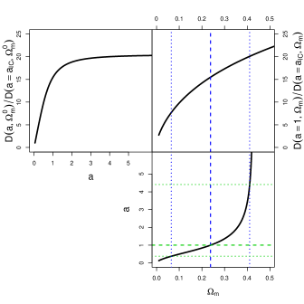
where is the linear growth function. In practice, we solve equation (2) numerically to get as demonstrated in Figure 1.
2.1.2 Approximate method for a single snapshot
Combining the two effects of expansion/compression and time-perturbations, the model for adding large-scale fluctuations to the mass density field is,
| (3) |
where is the mass over-density that would be measured in the all-modes simulation, is the mass over-density measured in the small-modes simulation, has zero power for , is defined by equation (2), and . Note that for this definition of the Zel’dovich displacements are added to the particle positions prior to application of the time-perturbation (i.e., at the positions at time , not at ). We will discuss this choice below.
When (which requires ) the first order correction to in should be sufficient for adding to the density field. Expanding both sides of equation (2) to first order in and ,
| (4) | ||||
Solving for gives,
| (5) |
which shows that the perturbed scale factor is roughly proportional to the large-scale density perturbations being added. Using equation (5) in the Taylor expansion of equation (3) gives,
| (6) |
This suggests that the addition of large-scale modes can be quickly computed given an estimate of the nonlinear growth rate of the small-modes simulation. With a single snapshot, the growth rate can be estimated from the continuity equation111Note that for simulation volumes Gpc on a side relativistic corrections to the continuity equation could be important. These arise from the way that the large scale potential perturbations modify the geodesic equations.,
| (7) |
and, using equation (3),
| (8) |
So, given particle positions and velocities at scale factor for a simulation that has no large-scale modes, equation (6) provides a method to add new large-scale mode realizations when the large-scale density perturbations are small.
According to equation (5) the range of is proportional to the range of . Because is Gaussian distributed by construction, we can determine the range of from its variance,
| (9) |
where is the fundamental frequency of the simulation box, is the theoretical dimensionless matter power spectrum, and is the Fourier transform of a spherical top-hat window of radius . The scale is roughly given by either the pixel scale of the gridded density field or the mean inter-particle spacing, whichever is larger. For the simulations we use below, , Mpc, and, with 2563 particles, . Evaluating equation (9) gives which is still less than as we required when choosing . But, as shown in Figure 1, the variations in greater than about lead to making equation (6) insufficiently accurate. In our test simulations actually varies over , giving a range of perturbed scale factor (shown by the dotted lines in Figure 1).
In Figure 2 we show the maximum value of as a function of the simulation box size while keeping fixed at 8 and, as in the preceding paragraph, assuming maximal variations in of .

For , as in the recently completed MXXL simulation222The MXXL simulation (Angulo et al. in preparation) was run by the Virgo Consortium (http://www.virgo.dur.ac.uk) in the spring of 2011. It is 3 Gpc on a side with particles with mass ., the variation in is less than 0.2 and the approximate formula in equation (6) could be sufficient for adding the large-scale modes to the small-modes simulation. To further assess the validity of equation (6), we show a histogram of the values of the third term in equation (6), normalized by , on a 5123 grid in our 1 Gpc small-modes simulation in Figure 3.
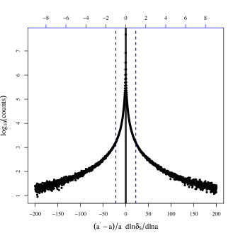
The distribution of grid cell values is strongly peaked around zero, but has wide tails extending to values of several hundred. This again illustrates that equation (6) is a bad approximation for a (1 Gpc)3 volume. However, if we scale the bin values on the lower horizontal axis by the ratio of the maximum perturbed scale factor in a (3 Gpc)3 simulation to the maximum in our simulation, we get the axis on the top of Figure 3. For a (3 Gpc)3 simulation 92% of the grid cells of the third term in equation (6) have values less than one. So, equation (6) may be a good enough approximation for adding large-scale modes to the MXXL or other simulations with similarly large volumes.
2.1.3 Full recipe
For box sizes smaller than several Gpc on a side, we need an algorithm that accurately implements the growth matching condition of equation (2) to compute the density in equation (3). For computational expediency and for later comparison with Takahashi et al. (2009), we have limited our test simulations to . Therefore, we have not tested the accuracy of equation (6). Instead, because our test simulation parameters yield , we apply the model of equation (3) by adjusting the positions of each particle in the simulation. If is the position of the th particle at scale-factor in the small-modes simulation, the model from equation (3) with modes added to the simulation can be rewritten for each particle position as,
| (10) |
where is the scale factor of the target time where the full density field (with new large-scale modes) is desired. That is, we first apply the same Zel’dovich displacement to the particle positions in all the snapshots (evaluated at the unperturbed positions in each snapshot). Then, we interpolate between these modified snapshots to find the particle position at perturbed time . To find the particle positions at all values of we must save simulation snapshots at times covering the range of values and spaced sufficiently closely in so that the interpolation of positions is accurate. This requires running the simulation far into the future ( for our test simulations) and saving ’s of snapshots, which creates both an extra computational and also a disk storage burden over the approximation in equation (6).
The steps of our full algorithm for adding large-scale modes to the small-scale density are then:
-
1.
Choose a threshold scale defining the boundary between large and small scale modes and a target time where the resampled density is desired.
-
2.
Calculate the range of perturbed scale factor defined by equation (2) about where the simulation snapshots will be required.
-
3.
Run an -body simulation in a periodic volume with nonzero Fourier modes in the initial conditions only for and save snapshots over the required range of that are spaced sufficiently close together to allow for accurate interpolation of particle positions.
-
4.
Calculate a new realization of large-scale modes on a grid.
-
5.
Calculate the Zel’dovich displacements defined in equation (1) from .
-
6.
Apply the Zel’dovich displacements to each snapshot of the small-modes -body simulation.
-
7.
Move each particle in the small=modes simulation to its location at time as defined by equation 2, interpolating between snapshots when necessary.
The resulting particle positions give a close approximation to the particle positions that would be obtained by running an -body simulation with the Fourier modes in present in the initial conditions (with the amplitudes suitably scaled according to the linear growth function).
The two operations of adding Zel’dovich displacements and perturbing the time where the particle positions are evaluated do not commute when the density field has evolved nonlinearly from the initial conditions. To decide on how to order these operations we imagine an approximation to an -body simulation where the initial conditions are first evolved by adding Zel’dovich displacements to the particles and then the density is scaled by the linear growth function. Reversing these operations, with the Zel’dovich move applied last, would be less analogous to the way the particle positions actually evolve in a simulation. In this latter scenario, the particles would first gravitationally collapse at rates determined by the local mean matter density and then at late times would undergo displacements to expand or compress regions in over- or overdense volumes. There is nothing physical about this ordering of operations. We have confirmed with our test simulations that the mode resampling does not work well unless the Zel’dovich move is the first step of the mode-resampling algorithm.
2.2. Algorithm implementation
The algorithm in Section 2.1 describes how to add large-scale Fourier modes to a simulation that had zero large-scale power in the initial conditions. Ideally we would like to first remove the existing large scale modes from a previously run simulation and then apply the algorithm in Section 2. We will discuss why this is challenging in Section 2.3, but first we describe details of the implementation of the mode addition algorithm.
To generate a simulation without large-scale power (what we call a “small-modes” simulation), we generated Gaussian Fourier mode realizations on a grid only for those modes, set all modes with to zero, and then performed the reverse Fourier transform to get the initial density field that is used for the first particle displacement step. We then evolve the simulation normally, but saving 43 snapshots equally spaced in over the range so the particle positions at perturbed times can be accurately determined by interpolating between snapshots. For testing purposes we ran another simulation using the same initial conditions, but before the large-scale modes were set to zero (called an “all-modes” simulation). The particle positions at in the all-modes simulation give our benchmark for testing the reconstruction of the density field when the large-scale modes that were deleted from the initial conditions are added back into the small-modes simulation at . Note that all the phases in the initial conditions were identical for both the all-modes and small-modes simulations. Unless otherwise specified, all our simulations were in box on a side with particles and were evolved using a lean version of the Gadget-2 code (Springel et al., 2001; Springel, 2005) from Gaussian initial conditions at redshfit 20.
Because gravitational evolution couples small-scale Fourier modes to the largest modes in the simulation box, the nonlinear perturbation growth rate in the small-modes simulation (i.e., with large-scale modes missing) is smaller than that in the all-modes simulation, as illustrated with the power spectrum comparison in Figure 4.
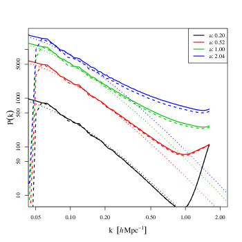
The solid lines show the power spectra of select snapshots in the all-modes simulation while the dashed lines show power spectra of the small-modes simulation at the same times (recall that the power spectra are equal in the initial conditions). At late times, the all-modes power spectrum has a significantly larger amplitude on small scales than the small-modes power spectrum. A first test of our mode-addition algorithm will be to correct for this deficit of nonlinear power.
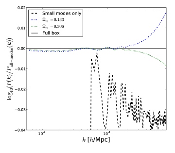
In order for the growth-matching condition in equation (2) to provide a useful means for correcting for missing large-scale power, the errors in matching the growth rate by perturbing the matter density must be much smaller than the change in the growth rate due to the ommission of large-scale power. We tested this condition explicitly by running two simulations with different values of and we plot their power spectra at matched linear growth in Figure 5. The power spectra in the two cosmologies match to % for wavenumbers Mpc, which is much less variation than between the all-modes and small-modes power spectra. This is why matching the linear growth is a good way to mimic the change in the local matter density.
We note that Zheng et al. (2002) have performed similar tests and showed that when the linear theory power spectrum is fixed (as we have assumed), several clustering statistics besides just the nonlinear power spectrum can be easily related between models with different and .
Next, we tested the various steps of the mode addition algorithm from Section 2.1 by matching the particle positions between the all-modes and the small-modes simulations by adding the large-scale modes from the all-modes initial conditions back into the small-modes simulation at (after scaling the large-scale modes by the linear growth function). Figure 6 illustrates our comparison for a section of the simulation volume. The black points show the particle positions in the all-modes simulation while red shows the positions in the small-modes simulation. It is readily apparent to the eye that both the time-perturbation and Zel’dovich moves are necessary to obtain a good match to the particle positions in the all-modes simulation.
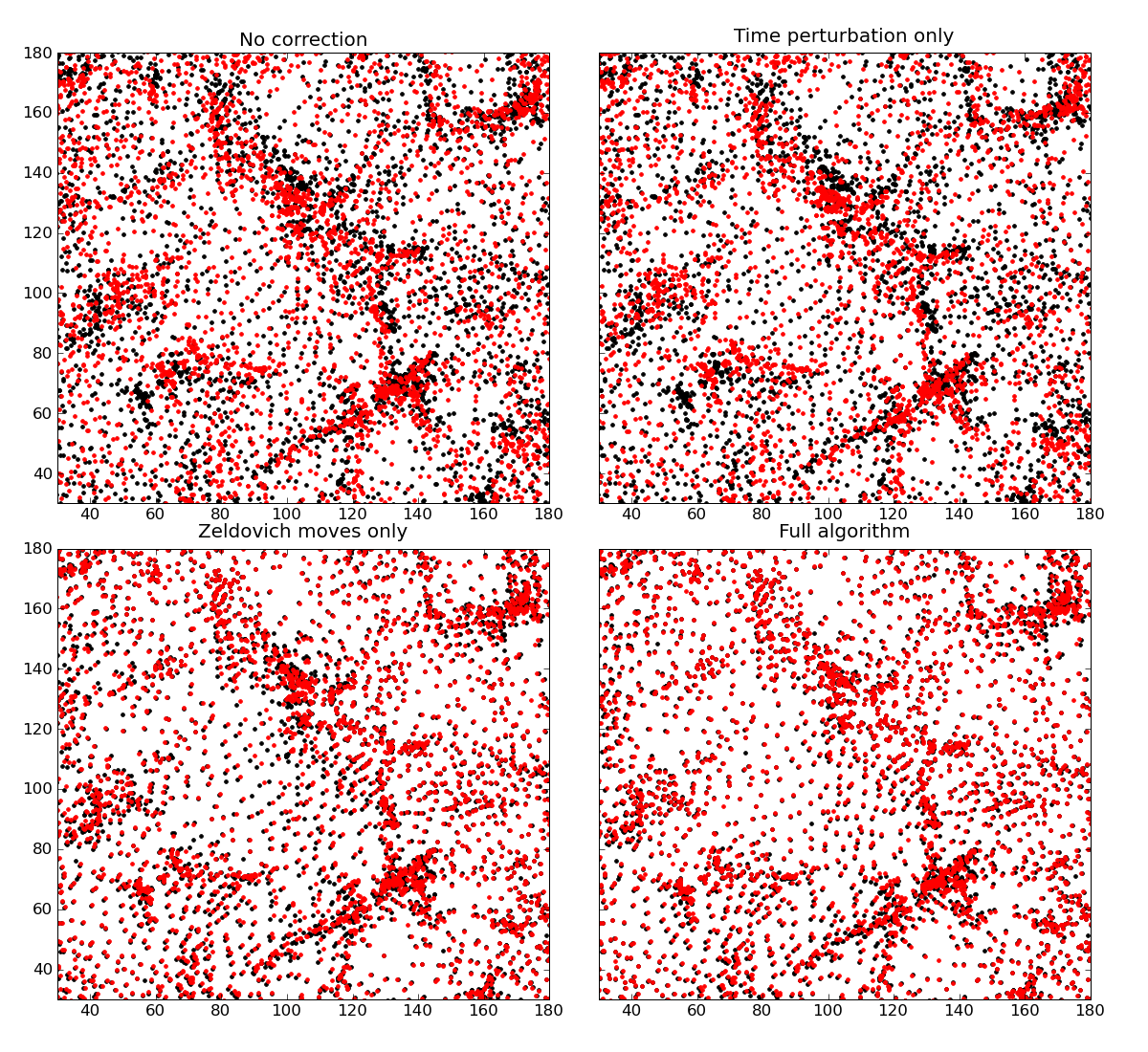
The Zel’dovich move alone does a better job matching the particle positions in the largest over-densities than the time-perturbation alone, but leaves significant position offsets compared to the final algorithm combining both perturbations.
2.3. Subtracting large-scale power
The algorithm we have demonstrated requires that an -body simulation be run with initial conditions that have the large-scale Fourier mode amplitudes set to zero and with a relatively large number of late time snapshots saved that can be used for interpolating particle positions. Ideally, we would like to have an algorithm that can be applied to existing -body simulations. Such an algorithm would first require a method for subtracting the large-scale modes already present in the simulation. Our procedure for adding large-scale modes should work in reverse, but with the new growth-matching condition,
| (11) |
We arrive at this condition by modeling regions where is overdense (overdense) as regions that have evolved without large-scale power but with a larger (smaller) local value of . We then find the time where a simulation with density and no large-scale power would have the same linear growth as the original simulation with density at time . However, removing the effect of large-scale under-densities can require evolving those overdense regions far into the future to match the growth on the right-hand side of equation (11). For CDM, the local linear growth in large under-densities can freeze and will never match the right-hand side in equation (11) even if evolved infinitely into the future. The growth matching condition in equation (11) and the problem with under-densities is illustrated in Figure 7.
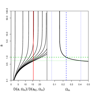
For our fiducial cosmology, , and all regions in that have density smaller than the mean density minus will be impossible to correct using the growth matching condition of equation (11). In the bottom panel of Figure 2 we show the maximum derived from equation (11) as a function of simulation box size assuming and that the maximum variations in are . For cubic simulation boxes with sides less than there is no solution for . For larger box sizes the maximum quickly decreases from to very close to one. So for simulation box sizes of several Gpc, removing large-scale modes may be feasible with minimal extra computational effort. However, again for computational expediency, we have limited our considerations in this paper to our Gpc simulations and therefore do not consider the removal of large-scale modes further.
3. Validation tests
We present further tests in this section to assess the accuracy of our method for introducing large-scale modes in -body simulations. We are primarily interested in the matter power spectrum and power spectrum covariance matrix and investigate estimators for these in turn.
3.1. Recovering the nonlinear power spectrum
In Figure 8 we demonstrate the reconstruction of the nonlinear power spectrum from the small-modes simulation. Using the all-modes simulation as our benchmark, we used the Fourier modes from the all-modes initial conditions with to determine the Zel’dovich moves and perturbed times for adjusting the small-modes simulation (so if our algorithm worked perfectly the power spectra should be perfectly matched). In addition to the CDM simulations described in Section 2.2, we ran analogous all-modes and small-modes simulations for an SCDM cosmology (i.e., with ). Because the SCDM model has no dark energy, the linear growth rate is completely determined by the matter density, and our growth matching condition in equation (2) should be an especially good approximation for the effect of large-scale Fourier modes on the gravitational growth rate.
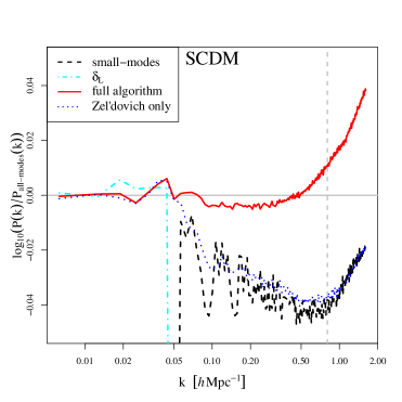
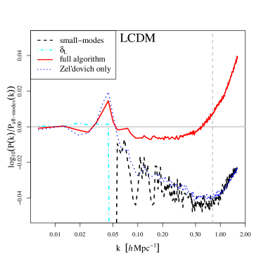
Figure 8 shows that the fractional errors in the reconstructed power spectra are indeed slightly smaller for the SCDM simulation, but the errors are much less than 1% for both cosmologies. Due in part to the cloud-in-cell deconvolution (which over-corrects the power on small scales), the fractional errors begin to increase significantly at about .
Note that the Zel’dovich correction alone, shown by dotted blue lines in Figure 8, does a very poor job of correcting the small-scale power spectrum for the added large-scale modes. This seems to be in contrast to the lower left panel of Figure 6 where the Zel’dovich correction alone appears to correct the particle positions rather well. We now see that the eye notices the agreement of large-scale structures more easily than the disagreement of small-scale structures in the dot plots of Figure 6.
3.2. Power spectrum covariance matrix
The gravitational growth of perturbations increases the small-scale power spectrum variance and induces significant correlations between power spectrum bands (Scoccimarro et al., 1999; Meiksin & White, 1999). In this Section we test how well our mode addition algorithm can reproduce these effects.
By perturbing a single small-modes simulation with independent Gaussian realizations of the large-scale modes, we can generate many realizations of the density field. These are not independent realizations because the small-scale modes are initially the same for each resampling. We use the covariance matrix estimated in Takahashi et al. (2009) from 5000 -body simulations to test our sample covariance estimates from simulations with resampled large-scale modes.
3.2.1 Sample covariance matrix estimator
First we define the estimator for the covariance matrix that we use for our comparisons.
Let denote the amplitude at grid point of the Discret Fourier Transform (DFT) of the density field from an -body simulation measured on a 3D uniform periodic grid. Then, the standard estimator for the power spectrum of the mode amplitudes is obtained by averaging over a spherical shell of constant radius ,
| (12) |
where is the number of modes that fit in the shell. We follow Takahashi et al. (2009) and set this shell thickness to . If we generate realizations of the density field (e.g. by running identical -body simulations except with different random number seeds to generate the initial conditions), the mean power spectrum estimator for all the realizations is:
| (13) |
The estimator for the covariance of the power spectrum from all the realizations is then:
| (14) |
Meiksin & White (1999), Norberg et al. (2009), and Takahashi et al. (2009) found that at least several hundred realizations of the matter density field are required to accurately estimate the sample covariance matrix. This means that hundreds (or thousands in some cases) of -body simulations must be run with different random number seeds in order to obtain a power spectrum covariance matrix estimate that is sufficiently accurate for cosmological parameter estimation.
3.2.2 Multiple power spectra from a single simulation box
Because running hundreds or thousands of -body simulations is often prohibitively expensive, previous studies have attempted to estimate the power spectrum covariance from a single -body simulation by applying window functions to the gridded density field to sub-sample the simulation volume. Hamilton et al. (2006) found that because the windows are convolved with the Fourier modes of the periodic simulation box, the resulting power spectrum covariance matrix estimates are significantly biased with respect to the result obtained from an ensemble of periodic simulations. Furthermore this bias cannot be simply accounted for by deconvolving the window functions from the power spectrum estimates, but is a result of higher order connected correlations entering the covariance matrix estimator, which Hamilton et al. (2006) call “beat-coupling.”
Although direct sub-sampling of the simulation volume has been shown not to reproduce the covariance from an ensemble of simulations, the idea that different regions of a large simulation volume provide statistically independent information about the small-scale covariance is sound if we accept the ergodic hypothesis and assume our simulation is big enough. To avoid the convolution in Fourier space imposed by the configuration-space windows of Hamilton et al. (2006), we attempted to sub-sample the Fourier modes that enter the shell-averaged power spectrum estimator in equation (13). For shells with large wavenumbers there are thousands of modes used to estimate the power spectrum. The nonlinear power spectrum covariance depends on the connected four-point correlations of the Fourier modes, but with thousands of modes on a uniform grid there must be many redundant four-point configurations that could yield independent samples of the (shell-averaged) power spectrum covariance (after appropriate scaling by the number of modes used to estimate the mean power spectrum).
The enumeration and counting of the four-point configurations in each shell is complicated, so we instead divided the surface of each wavenumber shell into uniform area HEALPix(Górski et al., 2005) pixels and then selected only one wavevector within each pixel to obtain a power spectrum estimate. For a given number of pixels covering the spherical shell, the minimum multiplicity of wavevectors in a pixel determines the number of pseudo-independent power spectrum estimates we can derive with this method. That is, if all pixels have at least wavevectors within their boundaries, then we can generate at most pseudo-independent realizations of the power spectrum estimates. We defined smaller (and therefore more) pixels for shells of increasing wavevector magnitude. This ensured that the multiplicity of each pixel was greater than one for a wide range in wavevector magnitudes.
We applied this sub-sampling to a small-modes simulation with 500 large-scale mode resamplings. The resulting power spectrum estimates and correlation coefficients of the estimated power spectrum covariance are shown in Figure 9.
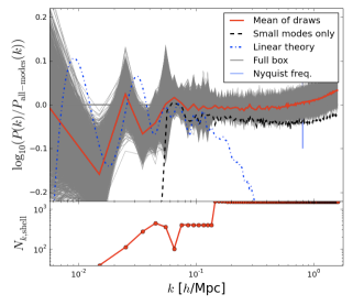
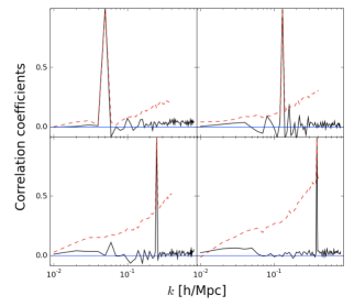
While the mean power spectrum is successfully recovered with this algorithm, the power spectrum covariance estimator has nearly zero off-diagonal terms, in stark contrast to the result from Takahashi et al. (2009) (shown in red, dashed lines) for wavenumbers Mpc-1. One explanation for this could be that our method of sub-sampling modes in the wavevector shells is not actually selecting representative samples of all the four-point configurations in each shell, which would be fixed by a more precise sub-sampling procedure.
Because pursuing this algorithm further would significantly increase the computational complexity while limiting the range of applications, we instead turned to using multiple small-modes simulations with large-scale mode resampling to further explore the covariance matrix estimates as described in the next Section.
3.2.3 Covariance matrix estimates from mode-resampling
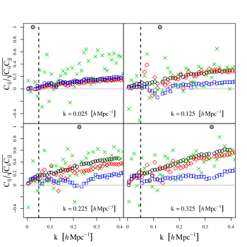
The power spectrum variance and correlation coefficients estimated from 500 resamplings of the large-scale modes in a single small-modes simulation are shown by the blue squares in Figure 10. Note that we use the same binning in wavenumber in all the cases shown as Takahashi et al. (2009) in order to make an accurate comparison.
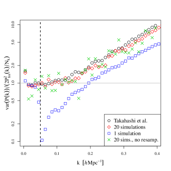
While the small-scale variance estimate is boosted beyond the Gaussian prediction, it is systematically biased low relative to the results of Takahashi et al. (2009). At intermediate wavenumbers just larger than , the estimated variance is only of the true value. This is not too surprising because it is at these scales where our algorithm for adding large-scale modes is expected to be most inaccurate. This is because our approximation that longer wavelength modes simply change the effective local matter density must be wrong when the longer-wavelengths are nearly equal to the smaller wavelengths to be perturbed. The modes just larger and smaller than may both contribute to coherent structures in the mass density distribution so that resampling only some of the Fourier modes in these structures would severely underestimate the true variance on these scales. Also, we should note that the modes with wavenumbers just smaller than are likely not strictly Gaussian distributed in the all-modes simulation, so that their true distribution and coupling to small modes is not properly represented.
The right panel in Figure 10 shows four rows of the matrix of estimated correlation coefficients of the power spectrum. It is significant that the mode resampling generates nonzero correlation coefficients between the large and small scales (blue crosses – lower panels especially), which are identically zero in the unperturbed small-modes simulation. However, the correlation coefficients are again biased low by multiplicative factors of two or more.
We have checked that the biases in the estimated power spectrum variance and correlation coefficients do not change when using more than 500 large-scale mode realizations. Instead we speculate that this bias is real and indicates that (at least for fixed ) the mode resampling algorithm generates realizations of the matter density from only a subset of the full nonlinear density probability distribution. This makes sense intuitively if we realize that the mode resampling as implemented here can never generate a new set of halos in the simulation box, but only moves and merges or de-merges the halos already present in the small-modes simulation. Several previous investigations have shown that the phase correlations in the Fourier modes of the density field in a dark matter simulation are dominated by the masses and positions of the most massive halos (Watts et al., 2003; Neyrinck & Szapudi, 2007). It makes sense then that the power spectrum variance on small-scales would also be quite sensitive to the particular realization of the most massive halos. However, with a larger simulation volume the covariance estimates might be less dependent on the particular realization of the massive halos because many different halo configurations would be present.
If our mode resampling algorithm is simply sampling a subset of the density probability distribution, then the bias in the power spectrum variance and correlation coefficients should decrease if we use more than one simulation. To check this hypothesis we ran 19 more small-modes simulations (for 20 total) with different random number seeds in the initial conditions and added 500 resamplings of the large-scale modes to each simulation (for a total of 10000 realizations of the density field). The sample covariance estimates improve considerably as shown by the red diamonds in Figure 10. The biases in both the variance and the correlation coefficients are much smaller over all scales. In addition, the extremely low dip in the variance estimates at intermediate scales when using only one simulation has disappeared entirely with 20 simulations.
Finally, we show an estimate of the covariance matrix using 20 simulations without any resampling of large-scale modes with the green crosses in Figure 10. With such a small number of simulations the statistical noise dominates in the estimator. Comparing with the estimator with 500 resamplings of each of the -body simulations shows how much our mode-addition algorithm reduces the statistical errors.
3.2.4 Convergence rate of covariance estimates
Although with 20 small-modes simulations the bias in the power spectrum covariance estimate is much smaller than with only one simulation, a small bias is still noticeable in Figure 10. In Figure 11 we attempt to quantify the improvement in the covariance matrix estimates as more small-simulations are added by plotting the r.m.s. dispersion in elements of the power spectrum variance relative to the result from Takahashi et al. (2009).
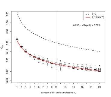
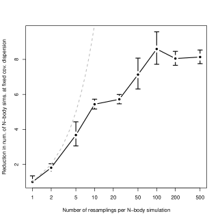
We show the distribution in the variance estimates for wavenumber bins with centers in with the boxes in the left panel of Figure 11. The horizontal lines in the centers of the boxes denote the median of the variance estimates and the box top and bottom denote the first and third quartiles. We have selected only high- modes to plot in Figure 11 because the variance estimate in this range has a roughly constant bias as seen in Figure 10 and we are primarily interested in the accuracy of the covariance estimates on small scales where the deviation from the Gaussian model is most severe. We show how the normalization of the fit to the covariance dispersion changes with the number of mode resamplings per -body simulation in the right panel of Figure 11. The reduction in the number of -body simulations needed to give a certain error in the estimate covariance flattens around 100 resamplings per simulation.
Takahashi et al. (2009) performed a similar analysis and found that the dispersion in their sample variance estimators was well fit by , where is the number of -body simulations (or realizations) used to compute the estimator (shown as the dashed black line in Figure 11). We find a nonlinear least squares fit to our variance estimates of , which is shown by the solid red line in Figure 11. From this we conclude that the sample variance estimator using resampled large-scale modes can achieve similar accuracy as the standard sample variance estimator but with times fewer -body simulations. However, it is difficult to extrapolate this convergence rate far beyond the 20 simulations we have actually performed because small changes in our choice of wavenumber bins or in our least-squares fit can cause large extrapolation errors.
4. Discussion and Conclusions
We have demonstrated an algorithm to resample the large-scale Fourier modes of the density in an -body simulation that successfully reproduces the nonlinear power spectrum and significantly reduces the number of simulations required to estimate the power spectrum covariance matrix. We expect our algorithm to aid the calculation of uncertainties for observational probes of the matter power spectrum such as weak lensing and galaxy clustering. Because we can quickly provide multiple realizations of the density field, it is possible to estimate uncertainties after applying appropriate survey windows to the density, which can have significant impacts on the estimated power spectrum covariances. This could be a distinct advantage over approaches that either precompute the power spectrum covariance without considering the survey window (Semboloni et al., 2007; Takahashi et al., 2009; Sato et al., 2009), or use approximate or analytic methods that may not include the survey windows correctly (e.g. Crocce et al., 2010). We have no reason to believe the extension to redshift space will pose any particular challenges. However, note that we have not yet tested the perturbation of the particle velocities so our results are limited to real-space statistics for now.
Our algorithm uses both Zel’dovich displacements as well as time-perturbations to match the effective local linear growth in over- or overdense regions. It is intriguing that neither of these operations alone is sufficient to reconstruct even the nonlinear power spectrum. Evaluating the time-perturbation at the particle positions prior to the Zel’dovich move gives a bad result, indicating that the early-time movement of the particles is significant in determining the later growth of structures. Any extensions of our algorithm will likely have to consider both of these components carefully.
Because applying the time-perturbation to remove large-scale modes from an existing simulation generally requires many simulation snapshots far into the future, we found it onerous (or even impossible if resampling too many modes in a box that is too small) to use existing simulations for mode-resampling. However, if the simulation volume is at least several Gpc on a side, then according to Figure 7 it may be possible to subtract a limited number of large-scale modes with a feasible amount of computation. For simulations volumes smaller than many Gpc on a side, we advocate running a new simulation with large-scale modes removed in the initial conditions, which can then have new large-scale modes added directly in later snapshots using our algorithm. Note that even for adding new large-scale modes the time-perturbation requires many snapshots closely spaced in scale factor both in the past and future of the desired time (but the simulation does not have to be run as far into the future as is needed for removing large-scale modes). This means that application of our algorithm for, e.g. parameter estimation from a galaxy survey, will require special-purpose -body simulations that will save significant computation time for the error analysis.
Our algorithm has other applications such as including scaling of halo masses and concentrations so that mock galaxy catalogues could be constructed from each of the resampled density fields. In our view, this is the only viable method to obtain robust uncertainties for estimating cosmological parameters from galaxy clustering and BAOs. Our algorithm may even provide a feasible method to go beyond the work of Sefusatti et al. (2006) for estimating the covariance of higher-order correlations. For parameter estimation with weak lensing, our resampled density fields could be directly input to existing ray-tracing pipelines. However, one would need resampled densities for each of the lens planes (which could extend to for upcoming survey requirements). This would require saving even more closely spaced snapshots of the small-modes simulation(s).
The sample covariance matrix estimated from a large number of resamplings of a single simulation has nonzero correlations between large and small scales that are introduced by our mode addition algorithm. But, the covariance elements are biased low relative to the benchmark result from Takahashi et al. (2009), which used 5000 -body simulations. A possible explanation for this bias is that our method of resampling large-scale modes samples only a subset of the full probability distribution for the nonlinear density field. We have shown that the bias decreases monotonically as a function of the number of -body simulations used to estimate the covariance, which is consistent with this explanation. If our mode-resampling algorithm were perfect at adding large-scale fluctuations, the bias in the covariance that we find would indicate that the distribution of the small-scale nonlinear density field is not entirely determined by the coupling with large-scale modes. Rather, the phases of the small-scale Fourier modes in the initial conditions would be important as well, which contradicts the conclusion of Little et al. (1991) who found little impact on the final nonlinear density when the small-scale phases were randomized in the initial conditions. This could be because the eye notices mostly the large-scale structures in a dotplot of the particle positions but there can be significant small-scale deviations that are less noticeable (as shown by the “Zel’dovich only” lines in Figure 8 versus the “Zel’dovich only” lower left panel of Figure 6).
One area for future investigation is to study the dependence of the bias in the power spectrum sample covariance (or other measures of the distribution of the nonlinear density) with . This would quantify the relative importance of different large-scale modes on the nonlinear density distribution. This could be a promising way to better understand the “loss” of information about cosmology in the matter power spectrum on translinear scales (Rimes & Hamilton, 2006; Neyrinck et al., 2006; Neyrinck & Szapudi, 2007). One could also quantify on which scales (if any) the density in a large simulation becomes ergodic (so that the distribution of the density in sub-volumes of the simulation is equivalent to the distribution of the density field in an ensemble of large simulations). The fact that our small-scale covariance estimates have such a large bias for Mpc (and in a single simulation) suggests that assuming ergodicity on these scales is a fallacy when defining estimators of, at least some, summary statistics of the density.
Another application of our algorithm could be for tiling smaller simulation volumes to obtain the (properly correlated) density field in volumes that are too large to simulate, as originally proposed by Cole (1997). This would probably be most effective if we run several of our “small-modes” simulations and then tile them together by resampling the modes both larger and smaller than the fundamental frequency of the simulation volume. A related application is re-running resimulation studies (that take a sub-volume of high-resolution -body simulation and add additional physics) with different large-scale mode realizations. This could be a relatively fast way to obtain different realizations of the resimulations with only one high-resolution -body simulation at hand.
Finally, we hope to apply our algorithm for obtaining estimates of both the mean power spectrum and its covariance as needed in simulation emulator frameworks (Heitmann et al., 2009; Schneider et al., 2011). Because we can estimate the power spectrum covariance with an easily achievable number of simulations, it will now be feasible to build an emulator for the cosmological-parameter dependence of the covariance (Schneider et al., 2008). Note that this paper is complementary to Angulo & White (2010) who described how to rescale the outputs of a single -body simulation to mimic the outputs with a different cosmology, but who did not consider the time-perturbations we use here. In combination, our algorithm and that of Angulo & White (2010) may serve to drastically reduce the number of simulations needed to construct simulation emulators for cosmological analysis.
Acknowledgments
We thank Adrian Jenkins for extensive technical advice on Gadget-2 and setup of initial conditions, David Weinberg for pointing us to his earlier related work, Alex Szalay for explanations of the growth of correlations in the Fourier phases of the density field, Yanchuan Cai for advice on applying perturbation theory to (an ultimately failed attempt to) add large-scale modes to our simulations and Mark Neyrinck, Bhuvnesh Jain, and Ravi Sheth for useful conversations. SMC acknowledges the support of a Leverhulme Research Fellowship. Some of the calculations for this paper were performed on the ICC Cosmology Machine, which is part of the DiRAC Facility jointly funded by STFC, the Large Facilities Capital Fund of BIS, and Durham University. This work performed under the auspices of the U.S. Department of Energy by Lawrence Livermore National Laboratory under Contract DE-AC52-07NA27344.
References
- Angulo & White (2010) Angulo, R. E. & White, S. D. M. 2010, MNRAS, 405, 143
- Cole (1997) Cole, S. 1997, MNRAS, 286, 38
- Crocce et al. (2010) Crocce, M., Cabre, A., & Gaztañaga, E. 2010, ArXiv e-prints
- Frenk et al. (1988) Frenk, C. S., White, S. D. M., Davis, M., & Efstathiou, G. 1988, ApJ, 327, 507
- Górski et al. (2005) Górski, K. M., Hivon, E., Banday, A. J., Wandelt, B. D., Hansen, F. K., Reinecke, M., & Bartelmann, M. 2005, ApJ, 622, 759
- Hamilton et al. (2006) Hamilton, A. J. S., Rimes, C. D., & Scoccimarro, R. 2006, MNRAS, 371, 1188
- Heitmann et al. (2009) Heitmann, K., Higdon, D., White, M., Habib, S., Williams, B. J., Lawrence, E., & Wagner, C. 2009, ApJ, 705, 156
- Lawrence et al. (2010) Lawrence, E., Heitmann, K., White, M., Higdon, D., Wagner, C., Habib, S., & Williams, B. 2010, ApJ, 713, 1322
- Little et al. (1991) Little, B., Weinberg, D. H., & Park, C. 1991, MNRAS, 253, 295
- Meiksin & White (1999) Meiksin, A. & White, M. 1999, MNRAS, 308, 1179
- Neyrinck & Szapudi (2007) Neyrinck, M. C. & Szapudi, I. 2007, MNRAS, 375, L51
- Neyrinck et al. (2006) Neyrinck, M. C., Szapudi, I., & Rimes, C. D. 2006, MNRAS, 370, L66
- Norberg et al. (2009) Norberg, P., Baugh, C. M., Gaztañaga, E., & Croton, D. J. 2009, MNRAS, 396, 19
- Pope & Szapudi (2008) Pope, A. C. & Szapudi, I. 2008, MNRAS, 389, 766
- Rimes & Hamilton (2006) Rimes, C. D. & Hamilton, A. J. S. 2006, MNRAS, 371, 1205
- Sato et al. (2009) Sato, M., Hamana, T., Takahashi, R., Takada, M., Yoshida, N., Matsubara, T., & Sugiyama, N. 2009, ApJ, 701, 945
- Schneider et al. (2011) Schneider, M. D., Holm, Ó., & Knox, L. 2011, ApJ, 728, 137
- Schneider et al. (2008) Schneider, M. D., Knox, L., Habib, S., Heitmann, K., Higdon, D., & Nakhleh, C. 2008, Phys. Rev. D, 78, 063529
- Scoccimarro et al. (1999) Scoccimarro, R., Zaldarriaga, M., & Hui, L. 1999, ApJ, 527, 1
- Sefusatti et al. (2006) Sefusatti, E., Crocce, M., Pueblas, S., & Scoccimarro, R. 2006, Phys. Rev. D, 74, 023522
- Semboloni et al. (2007) Semboloni, E., van Waerbeke, L., Heymans, C., Hamana, T., Colombi, S., White, M., & Mellier, Y. 2007, MNRAS, 375, L6
- Smith et al. (2003) Smith, R. E., Peacock, J. A., Jenkins, A., White, S. D. M., Frenk, C. S., Pearce, F. R., Thomas, P. A., Efstathiou, G., & Couchman, H. M. P. 2003, MNRAS, 341, 1311
- Springel (2005) Springel, V. 2005, MNRAS, 364, 1105
- Springel et al. (2001) Springel, V., Yoshida, N., & White, S. D. M. 2001, New Astronomy, 6, 79
- Takada & Jain (2009) Takada, M. & Jain, B. 2009, MNRAS, 395, 2065
- Takahashi et al. (2009) Takahashi, R., Yoshida, N., Takada, M., Matsubara, T., Sugiyama, N., Kayo, I., Nishizawa, A. J., Nishimichi, T., Saito, S., & Taruya, A. 2009, ApJ, 700, 479
- Tormen & Bertschinger (1996) Tormen, G. & Bertschinger, E. 1996, ApJ, 472, 14
- Watts et al. (2003) Watts, P., Coles, P., & Melott, A. 2003, ApJ, 589, L61
- Zel’dovich (1970) Zel’dovich, Y. B. 1970, A&A, 5, 84
- Zheng et al. (2002) Zheng, Z., Tinker, J. L., Weinberg, D. H., & Berlind, A. A. 2002, ApJ, 575, 617