The Cosmic Linear Anisotropy Solving System
(CLASS) III: Comparision with CAMB for $\Lambda$CDM

Abstract:

By confronting the two independent Boltzmann codes CLASS and CAMB, we establish that for concordance cosmology and for a given recombination history, lensed CMB and matter power spectra can be computed by current codes with an accuracy of 0.01%. We list a few tiny changes in CAMB which are necessary in order to reach such a level. Using the common limit of the two codes as a set of reference spectra, we derive precision settings corresponding to fixed levels of error in the computation of a CMB likelihood. We find that for a given precision level, CLASS is about 2.5 times faster than CAMB for computing the lensed CMB spectra of a $\Lambda$CDM model. The nature of the main improvements in CLASS (which may each contribute to these performances) is discussed in companion papers.

1 Introduction

In a few companion papers [1, 2], we expose the main motivations for developing and releasing a new Boltzmann code, the Cosmic Linear Anisotropy Solving System (CLASS). Our targets are (i) friendliness and flexibility, (ii) a full control of errors, (iii) computational speed, (iv) to get an opportunity to test the accuracy of other codes with an independent one. In this paper, we will focus on the last three aspects. Since CAMB [3] is the only public code which has been regularly maintained over the past few years (including important updates on the recombination side), and since it is completely independent from CLASS (see however the disclaimer below about recombination), we only compare here CLASS with CAMB (last available version of January 2011). For a recent comparison between CAMB and CMBFAST [4], which are not completely independent, we refer the reader to ref. [5]. Precision tests for CMBEASY were presented in [6], and for other codes in [7]; however, these last two papers are now out-dated: since 2003, significant progresses were made on the side of recombination, lensing calculation, etc.; besides, in these previous papers, the accuracy of the codes was pushed to a much smaller level than in [5] and in the present work. The authors of [7] showed that the unlensed CMB spectra of several codes agree almost to the 0.1% level. This observation was crucial for interpreting WMAP data, but for Planck and post-Planck data (CMB, cosmic shear surveys, etc.) we would like to push the comparison further, in order to derive reference settings in which the theoretical error is proved to be much smaller than the observational error.

Hence, the first goal in this paper is to check the agreement between CLASS and CAMB , and to identify possible systematic errors induced by one or both of them. This investigation is presented in section 2. The discrepancy which will remain after tracking all possible sources of inaccuracy will give an estimate of the absolute precision of current Boltzmann codes. Up to this level of accuracy, the spectra produced by any of the codes can be treated as reference spectra. The most robust way to estimate the accuracy of CLASS or CAMB for a given set of precision parameters is to compare the output spectra with these reference spectra. In section 3, we will use this method for establishing a few sets of well-calibrated precision parameter sets. Finally, in section 4, we will compare the speed of the two codes for a fixed level of accuracy.

For concision, we restrict this work to the consideration of minimal $\Lambda$CDM models, and to the calculation of the CMB spectra and matter power spectrum $P(k)$ for scalar modes with adiabatic initial conditions. Within the small range of $\Lambda$CDM parameters allowed by current cosmological data, there is no reason for which the precision of the code would vary significantly with the cosmological parameters: hence, we can base our entire comparison on just one set of cosmological parameters close to the best-fit concordance model. The CLASS vs. CAMB comparison for isocurvature modes, tensors or extended cosmologies (e.g. with spatial curvature or massive neutrinos) is left for future specialised communications (the case of massive neutrinos and non-cold dark matter relics is already discussed in a companion paper [8]).

In our estimate of the speed of the code, we will focus only on the running time needed on one CPU for computing the CMB spectra in a $\Lambda$CDM model. Any other comparison (including the matter power spectrum, massive neutrinos, parallel runs, etc.) is likely to be even more in the favor of CLASS, thanks to its extended approximation schemes dealing with simplified equations during matter domination [2], with fluid approximations for non-cold relics [8], with its advanced stiff integrator [2], with its large amount of parallelised loops, etc.

Of course, the physical equations integrated in CLASS and CAMB in absence of any approximation scheme are the same, and CLASS uses the exact “line-of-sight integral method” proposed by Seljak & Zaldarriaga [4] and implemented in CMBFAST , CAMB and CMBEASY . CLASS and CAMB are still independent from each other in the sense that everything in CLASS apart from the recombination module has been written from scratch in another language, using different overall architecture, numerical algorithms, discretisation schemes, approximations, etc. Apart from the exact physical equations, the only common block is the module RECFAST [9] (currently at version 1.5 [10]) which computes the recombination history for a given set of cosmological parameters. In CLASS, the Fortran version of RECFAST v1.5 has been translated into C; it has then been slightly modified by introducing smoothing functions in order to avoid discontinuities in the derivatives of thermodynamical variables (this turns out to be useful, see the related discussion in section 2.1); but apart from smoother transitions between various approximation schemes, the equations of RECFAST are unchanged.

Simulating recombination is a tough problem which has its own level of uncertainty. Experts agree that RECFAST v.1.5 is accurate enough for analysing Planck data, but it is clear that in this paper, we will push the precision of the two Boltzmann codes at a level comparable or even larger than the expected precision of RECFAST. As long as CLASS and CAMB use the same recombination code, it is possible to compare them up to arbitrarily high level. But it should be clearly understood that the goal of this paper is to estimate the accuracy of CLASS and CAMB for a given recombination history. For concision, we will not write such a disclaimer in all relevant places in the text. Estimating the propagation of uncertainties from recombination to the CMB spectra is an independent task, actually requiring negligible errors from the Boltzmann code itself. In order to extract cosmological parameters from highly accurate data (like that from Planck or from future cosmic shear surveys), cosmologists need to be sure that neither recombination nor Boltzmann codes can introduce significant errors. The present work is only addressing the Boltzmann side.

2 Agreement with CAMB 

All along this work, we fix the $\Lambda$CDM cosmological parameters to typical $\Lambda$CDM values, and vary the precision parameters of CAMB and CLASS. We first need to check that each code tends towards stable results when the precision increases, and that the limits from the two codes agree with each other. If this turns out to be the case, we will conclude that the codes are not plagued by bugs or numerical issues, and we will be able to interpret the obtained spectra as “reference spectra”. Such a conclusion is correct provided that the two codes do not contain the same mistake, which would be very unlikely since they are independent (in the sense discussed in the introduction).

We start by tuning each CLASS precision parameter one by one, up to a level at which the CMB spectra (unlensed/lensed temperature and E-polarisation, plus lensing potential spectrum) remain stable at the $0.01\%$ level in the range $2-3000$ (settings called [CLASS:01]). The corresponding precision parameter values can be found in the input file cl_ref.pre of the public distribution of the code (as explained in [1], CLASS can be ran with two input files, one for cosmological parameters, and one for precision parameters: for instance, ./class my_model.ini cl_ref.pre).

2.1 Scalar unlensed CMB spectra

Next, we run CAMB with the following precision parameters (settings called [CAMB:01]):

l_max_scalar	=	3000
k_eta_max_scalar	=	12000
accurate_polarization	=	T
accurate_reionization	=	T
do_late_rad_truncation	=	F
accuracy_boost	=	3
l_accuracy_boost	=	3
l_sample_boost	=	3

Note that setting all accuracy boost parameters to three is often used in projects requiring high precision. Above, the parameter k_eta_max_scalar is set to four times l_max_scalar, while the default recommendation is just two times. Hence, we expect these settings to be very accurate.

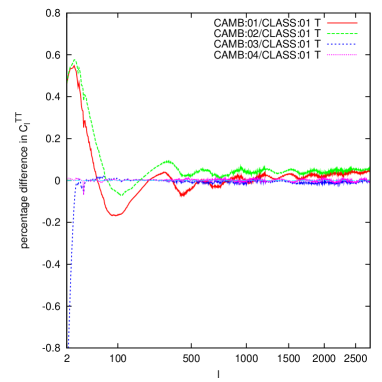
We find nevertheless a small discrepancy in the unlensed temperature multipoles $C_{l}^{TT}$’s, of the order of 0.7% at small $l$, and 0.1% at large $l$ (see figure 1, left plot, curve labelled CAMB:01/CLASS:01 T). At this point, further increasing CAMB’s “accuracy boost” parameters does not affect the results anymore. Note that these parameters control most precision parameters in CAMB, but not all of them: several quantities are fixed by hand inside each CAMB module. We tried to identify these quantities, to vary them one by one, and to check whether they have a sizable impact. This turns out to be the case for at least two numbers controlling:

1. the sampling of Bessel functions. CAMB samples spherical Bessel functions $j_{l}(x)$ with four different linear steps in four intervals in $x$. For values $x>25$, $\Delta x$ is set to one. We reduced this value to 0.2 (settings called [CAMB:02]) and found that the $C_{l}$’s are affected by approximately 0.1% (see figure 1, left plot, curve labelled CAMB:02/CLASS:01 T).

2. the sampling of the free electron fraction $x_{e}(\tau)$ along conformal time $\tau$, in view of computing the visibility function $g(\tau)$.

This second issue deserves more explanations. In CAMB, thermodynamical quantities are computed in the following way:

• the RECFAST module (version 1.5) computes the free electron fraction and baryons sound speed ($x_{e}(\tau)$, $c_{b}^{2}(\tau)$) by integrating the Boltzmann equations describing helium and hydrogen recombination over Nz linear steps in redshift space, between $z=z_{\text{max}}$ and $z=0$. By default, $z_{\text{max}}$ = Nz = 10’000, so the integration step is $\Delta z=1$.

• the functions $x_{e}(\tau)$ is corrected to account for reionisation (but the function $c_{b}^{2}(\tau)$ is not, as we shall see in subsection 2.3).

• CAMB’s “ThermoData” module computes derived (and integrated) quantities like the opacity $\kappa^{\prime}$, the column density $e^{-\kappa}$, the visibility function $g=\kappa^{\prime}\exp[-\kappa]$ and its time-derivatives. This last step is performed using another linear sampling of these functions: the number of points between $z_{\text{max}}$ and $0$ is then fixed by the integer nthermo. By default, nthermo = Nz = 10’000, so that the RECFAST and ThermoData modules use the same sampling.

In CLASS, the step (a) is identical to CAMB. The step (b) is also roughly similar, except for the choice of $z$ sampling near the reionisation epoch (found automatically for a given reionisation function), and the fact that we ensure that $x_{e}(\tau)$ remains exactly continuous and derivable at any time. The baryon sound speed is only computed after this step. Finally, for the (c) step, CLASS always uses the $z$ sampling defined at steps (a) and (b).

By inspecting the thermodynamical quantities as a function of redshift, we find that CAMB and CLASS agree very well as far as the free electron fraction and opacity are concerned, while there are small offsets in integrated and derived quantities like $e^{-\kappa}$ and $g$. This signals some inaccuracy in the numerical integration, derivation or interpolation routines used in at least one of the two codes.

In order to check for the convergence of CAMB’s thermodynamical variables, we would like in principle to increase the values of Nz and nthermo. In practise, increasing Nz is not possible due to the little discontinuities in the $x_{e}(\tau)$ and $x_{e}^{\prime}(\tau)$ functions returned by the raw version of RECFAST v1.5: as soon as the step decreases, spurious oscillations appear in all derived quantities, and the final results diverge. However, it is possible to keep Nz fixed and to increase nthermo, in order to check that the integration/derivation of the function $x_{e}(\tau)$ returned by RECFAST is accurate enough. We find that pushing nthermo in the range 80’000-100’000 leads to stable results, which are significantly different from those with the default setting nthermo=10’000. Moreover, the new results are in excellent agreement with the high-precision limit from CLASS. Note that increasing nthermo but not Nz has the inconvenient effect of introducing little oscillations due to spline interpolation, but they seem harmless for nthermo $\sim$ 100’000, since the spectrum does converge towards the one of CLASS.

This suggest that in CAMB, nthermo should always be kept of the order of 100’000 in order to gain one order of magnitude in precision (from the 0.1% to the 0.01% level). At this step, there is still a loophole in our reasoning. It might be the case that the two codes agree by coincidence when nthermo=100’000. Since we could not push Nz above 10’000 and nthermo above 100’000, we have not proved that the final result is fully converged with the settings Nz = 10’000, nthermo=100’000.

Fortunately, this question can be addressed. Here comes into play the fact that the RECFAST implementation in CLASS has a small difference with respect to the one in CAMB and the original one: it includes smoothing functions in the system of differential equations, which ensure that $x_{e}(\tau)$ is everywhere continuous and twice derivable. These smoothing function do not affect $x_{e}(\tau)$ in a detectable way. One can check it by changing the details (width and shape) of the smoothing functions: this impacts the final results at a level much below the 0.01% level. Hence, the fact that CLASS contains such smoothing functions is not a possible explanation for the small discrepancy discussed in the previous paragraphs.

If the impact of these smoothing functions is negligible, why did we introduce them at all? The reason is purely numerical. CLASS has a unique parameter recfast_Nz which plays the role of both Nz and nthermo in CAMB. When we increase this parameter, we increase the precision of the thermodynamics module without getting spurious features, thanks to the smoothing functions. In other words, the smoothing does not affect physical assumptions, but allows to test convergence. When we increase recfast_Nz much above 100’000 in CLASS, the output spectrum remains very stable (it varies by much less than 0.01%). This is indeed a proof that CLASS with recfast_Nz=100’000, or CAMB with Nz=10’000 and nthermo=100’000 are both fully converged from the point of view of thermodynamical quantities, at least at the 0.01% level.

The residual difference between CAMB with nthermo increased to 100’000 (setting [CAMB:03]) and CLASS (settings [CLASS:01]) is shown in figure 1, left plot, blue curve. The difference is now sensitive to an additional increase in CAMB’s “accuracy boost” parameters up to

accuracy_boost	=	12
l_accuracy_boost	=	4
l_sample_boost	=	3

(settings [CAMB:04]). The results from [CAMB:04] and [CLASS:01 T] agree at a rather spectacular level of $0.01\%$ for $C_{l}^{TT}$ in the range $2-2000$. The only exception is the multipole $l=18$, for which the codes agree only at the $0.07\%$ level. This detail is in any case completly irrelevant for practical purposes. Note that CAMB’s parameter do_late_rad_truncation can be indifferently set to T or F without affecting our conclusions: it governs an approximation which affects only the evolution of small scale perturbations after recombination, and do not impact significantly CMB observables.

For the same settings, the agreement between the polarisation spectra $C_{l}^{EE}$’s is roughly as good as for temperature: the spectra differ at most by $0.02\%$ in the range $40-3000$, or $0.04\%$ in the range $3-40$ ($0.14\%$ for $l=2$). The comparison between [CAMB:04] and [CLASS:01] results for TT and EE is shown on the right plot in Figure 1.

Figure 1: (Left) percentage difference between CAMB and CLASS unlensed temperature anisotropy spectra $C_{l}^{TT}$, for different precision settings for CAMB, explained in the text. (Right) best agreement reached in this work between CAMB and CLASS, for unlensed temperature and E-polarisation $C_{l}$’s.

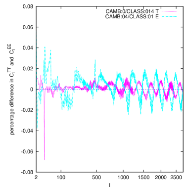
The agreement between the two codes could probably be pushed even further. We strongly suspect that the dominant source of error remains in the sector of thermodynamical quantities, especially for CAMB. Even without changing any physical assumption about recombination, the numerical accuracy could be increased by dealing with issues of sampling, discontinuities, derivation algorithms, etc. We did not pursue along this direction, which is somewhat involved and probably not justified, since $0.01\%$ or $0.02\%$ errors in the $C_{l}$’s are far below the sensitivity of realistic experiments (we will see in section 3 that for Planck’s effective chi square, $\chi^{2}\equiv-2\ln{\cal L}$, such errors lead to $\Delta\chi^{2}\sim 0.03$ only).

We conclude that current Boltzmann codes are able to predict the $C_{l}$’s with an accuracy of the order of 0.01% for a fixed recombination history. As mentioned in the introduction, physical uncertainties on recombination, on which Boltzmann codes have no control, are clearly the major source of error in the computation of CMB spectra.

Of course, in order to reach such an accuracy, CAMB and CLASS are both extremely slow (each run would require one or two days for each model on a single processor; of course, we performed these runs in parallel on many cores). The goal of section 3 will be to degrade the precision and to speed up the two codes, with a possibility to control the error by comparing with the reference spectra derived in this section.

2.2 Lensing potential and lensed CMB

The lensing potential multipoles $C_{l}^{\phi\phi}$ converge very slowly as a function of the large-wavenumber cut-off in the integration of transfer functions, parametrised in both codes by a parameter $(k\tau_{0})_{\text{max}}$ ($\tau_{0}$ being the conformal age of the universe). In order to obtain stable results at the 10% level for $C_{l}^{\phi\phi}$ around $l\sim 3000$, one would need to set $(k\tau_{0})_{\text{max}}$ to at least 15000. Reaching such an accuracy at $l=3000$ does not make much sense physically, since for such angular scales the non-linear corrections are expected to be of the order of a factor two. For comparison purposes, we fixed $(k\tau)_{\text{max}}$ to 12000 in both CLASS (settings [CAMB:04]) and CAMB. With this setting, the absolute value of linear $C_{l}^{\phi\phi}$’s around $l=3000$ is not per-cent accurate, but the results from the two codes should in principle agree very well since the cut-off is the same in the two cases. The error made by both codes on high-$l$ $C_{l}^{\phi\phi}$’s is not worrysome, since it does not propagate to the lensed CMB spectra. This is easy to check explicitly: by varying $(k\tau_{0})_{\text{max}}$, we established that the setting $(k\tau_{0})_{\text{max}}=12000$ is indeed sufficient for obtaining stable lensed CMB spectra in the range $l=2-3000$ at the 0.01% level.

In view of computing the lensed $C_{l}$’s up to $l=3000$, we need the $C_{l}^{\phi\phi}$’s up to a higher $l$’s, even if they do not need to be very accurate. In the settings [CAMB:05], we increase l_max_scalar from 3000 to 4000. The settings [CLASS:01] don’t need to be changed, because CLASS automatically increases $l_{\text{max}}$ by an amount delta_l_max when lensed $C_{l}$’s are requested. In the [CLASS:01] settings, delta_l_max is fixed to 1000, so that $l_{\text{max}}$ is also increased to 4000.

CLASS computes the lensed CMB spectra from all-sky correlation functions [12], i.e with the same method as CAMB, but with a different numerical implementation written by S. Prunet, based on quadrature weigths.

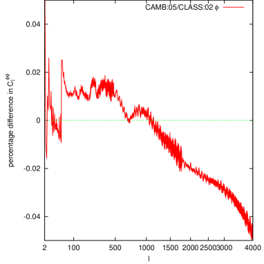
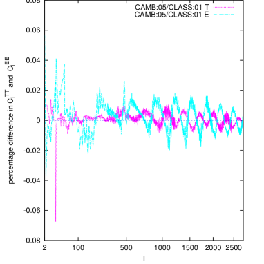
We compare the $C_{l}^{\phi\phi}$ spectra from the [CAMB:05] and [CLASS:01] in figure 2 (Left). The two spectra agree at the level of $0.025\%$ in the range $3-4000$ (and $0.07\%$ for $l=2$): this is (by far) good enough in order to get accurate lensed temperature/polarisation multipoles. Indeed, sticking to the same precision settings, we compare the lensed temperature and polarisation spectra in the range $2-3000$ in figure 2 (Right). Nicely, the agreement remains as good as for the unlensed spectra (by $0.01\%$ for temperature excepted at $l=18$, and by $0.02\%$ for polarisation for $l\geq 40$).

Figure 2: (Left) percentage difference between CAMB and CLASS lensing potential anisotropy spectra $C_{l}^{\phi\phi}$, with the precision settings explained in the text. (Right) percentage difference between CAMB and CLASS lensed temperature anisotropy spectra (temperature TT and polarisation EE).

2.3 Matter power spectrum

In the standard cosmological scenario, the matter power spectrum can be accurately described by linear theory up to about $k\sim 0.1\,h$Mpc^-1. Hence, one could argue that precise computations of the matter power spectrum $P(k)$ for larger wavenumbers are useless. Nevertheless, we want to push the comparison up to much higher values, because the small-scale linear power spectrum is often used as an input for different methods estimating the non-linear spectrum: fitting formulas like HALOFIT [11], codes generating initial conditions for N-body simulations, algorithms computing renormalised perturbations, etc. In this paper we focus on the matter power spectrum in the range $10^{-4}h\,$Mpc${}^{-1}<k<50\,h\,$Mpc^-1.

The settings described in the previous subsections are sufficient in order to get accurate predictions in the range from $10^{-4}$ to $1h\,$Mpc^-1. Beyond that, it is necessary to increase the number of Legendre multipoles for massless neutrino perturbations, $l_{\nu\text{max}}$, in order to follow accurately neutrino free-streaming during radiation domination (when their backreaction on metric perturbations cannot be neglected). In CLASS, $l_{\nu\text{max}}$ can be kept not too large thanks to the Ultra-relativistic Fluid Approximation (UFA) described in ref. [2]. The precision parameter file pk_ref.pre released with CLASS has $l_{\nu\text{max}}$=150. Together with other settings, this is found to be sufficient for $P(k)$ to converge at the $10^{-5}$ level, up to at least $k_{\text{max}}=50\,h\,$Mpc^-1. We refer to CLASS runs with the accuracy file pk_ref.pre as [CLASS:02].

We compared the resulting $P(k)$ with that derived from CAMB with the following settings, that we call [CAMB:06]:

transfer_high_precision	=	T
accuracy_boost	=	3
l_accuracy_boost	=	3
do_late_rad_truncation	=	T

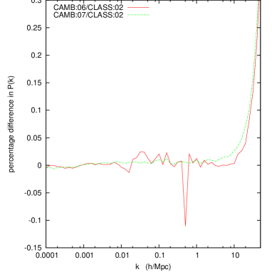
Other relevant parameters have been set to the same values as in the previous [CAMB:05] settings (including nthermo=100’000). The result of the comparison, shown in fig. 3 (Left), exhibits a few features at the level of 0.1%, plus a very sharp raise above $1h\,$Mpc^-1. We tried to turn off CAMB’s do_late_rad_truncation approximation and to increase accuracy boost parameters until the matter power spectrum converges up to the $10^{-5}$ level. This occurs for the settings

transfer_high_precision	=	T
accuracy_boost	=	5
l_accuracy_boost	=	8
do_late_rad_tr-unction	=	F

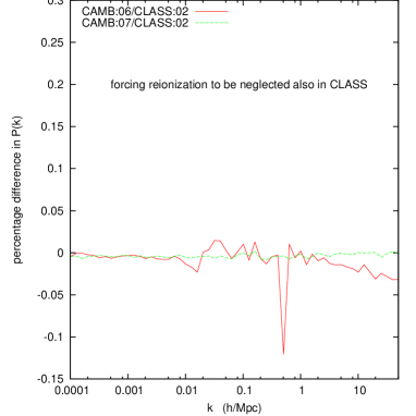
that we call [CAMB:07]. The large value of the l_accuracy_boost parameter reflects the need to increase $l_{\nu\text{max}}$, especially in absence of an UFA approximation. At this point, the two matter power spectra agree up to the 0.01% level up to $1h\,$Mpc^-1, but the sharp raise persists in the large-$k$ limit. A careful inspection shows that this effect comes entirely from the fact that CAMB neglects the impact of reionisation on the baryon sound speed $c_{s}^{2}(z)$, while CLASS sticks to the equations from [13] which assume thermal equilibrium between baryons and electrons. Indeed, CAMB infers the baryon sound speed from the free electron fraction immediately after calling RECFAST , while CLASS uses the free electron fraction already corrected by the effect of reionisation. Hence, at low redshift, $c_{s}^{2}$ is one order of magnitude larger in CLASS; the Jeans instability of baryons is then responsible for a cut-off in the matter power spectrum not far from $k\sim 10h\,$Mpc^-1. We checked in fig. 3 (Right) that if we run CLASS with the same cosmological parameters but reionisation switched off, the results of [CAMB:07] and [CLASS:02] agree at the 0.01% level at least till $k=50h\,$Mpc^-1.

Of course, in the non-linear power spectrum and near the wavenumber $k\sim 50h\,$Mpc^-1, the cut-off is erased by the transfer of large-scale to small-scale power. So, in practice, this difference between the two codes (which both oversimplify the baryon evolution during reionisation in different ways) is not a problem.

Figure 3: (Left) percentage difference between CAMB and CLASS matter power spectrum $P(k)$, with the precision settings explained in the text. (Right) same if we force CLASS to neglect the impact of reionisation on the baryon sound speed, like CAMB does.

3 Precision settings

The settings [CLASS:01] and [CLASS:02] can be used to produce reference spectra, and then to calibrate different degraded precision settings, adapted to the user’s goal. In the distribution of CLASS v1.0, these settings correspond to the precision files cl_ref.pre and pk_ref.pre. We recall that the first one is sufficient for getting 0.01% accurate $C_{l}^{TT}$’s and $P(k)$’s in the range $2\leq l\leq 3000$ and $k\leq 1h\,$Mpc^-1 (for $C_{l}^{EE}$ the error is twice larger). The second settings is only necessary for maintaining such an accuracy on the linear $P(k)$ till $k\leq 50h\,$Mpc^-1.

Under many circumstances, a Boltzmann code user wants to be sure that the error made on the $C_{l}$’s is smaller than some level (e.g., than the level of the new physical effect that he/she wants to study). For this purpose, we derived three settings achieving respectively 0.1%, 0.2% or 0.3% accuracy on the $C_{l}$’s up to $l=3000$: they are contained in the precision files cl_permille.pre, cl_2permille.pre, cl_3permille.pre distributed together with the code. For each of these settings, the precision on the matter power spectrum for $k\leq 1h\,$Mpc^-1 is even better than that on the $C_{l}$’s.

However, for parameter extraction and large Monte-Carlo runs, these settings are not optimal: they do not minimise the computing time for a given data sensitivity. In principle, for each new data set, one could derive optimal precision settings for CLASS. The way to proceed is to compute some reference spectra using e.g. the cl_ref.pre file, and then to degrade the precision while keeping the likelihood of the output spectra below a given level (given instrumental noise and taking the fiducial spectra to be the reference ones).

Here, we illustrate this approach by using a simplified Planck likelihood. In the future, it will be easy to derive e.g. “Planck+SDSS” or “Core+Euclid” precision files. This task is made easier if one assumes that each accuracy parameter degrades the precision independently of the others, i.e. that no complicated combinations of the accuracy parameters can make the code faster for a fixed precision. Under this very plausible assumption, deriving precision settings is trivial, even for somebody who is not expert in the code: one should consider the accuracy parameters one after each other, loop over several values of these parameters, compute the $\Delta\chi^{2}$ relative to the reference spectrum, and take the largest possible value of each accuracy parameter compatible with a given order of magnitude for $\Delta\chi^{2}$ (here $\chi^{2}$ is defined to be $-2\ln{\cal L}$, and ${\cal L}$ is the likelihood of a combination of experiments). The role of each precision parameter is summarised in the comments of the CLASS file ${\tt include/common.h}$, where all precision parameters are declared within a structure called precision.

For illustration, we assume here a simplistic Planck likelihood based on three channels, with a gaussian isotropic noise and a fraction of the sky $f_{\text{sky}}=0.8$. Details on this likelihood can be found e.g. in [14]. The instrumental noise from Planck increases exponentially above $l=2500$, but throughout this comparison exercise we compute the $\chi^{2}$ up to 3000, even if the last mutipoles do not contribute much. In order to obtain some $C_{l}$’s at $l=3000$, we must keep ${\tt l\_max\_scalar}$ higher than 3250 in CAMB .

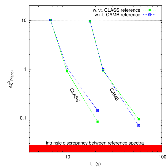
We first checked that the CLASS and CAMB reference CMB spectra presented in the previous section differ by $\Delta\chi^{2}=0.027$: we conclude that given the current accuracy of Boltzmann codes, the effective $\chi^{2}$ obtained with Planck will only be accurate up to 0.03. Fortunately, this precision is by far sufficient for extracting cosmological parameters in a robust way, without introducing any sizeable “Boltzmann code bias”.

We then degrade the precision of the two codes as much as possible in order to keep the error below $\Delta\chi^{2}\sim 0.1$, 1 or 10. During this step, we compute the $\Delta\chi^{2}$ relative to the CLASS reference spectra, but it would be equivalent to define it with respect to the CAMB one. Let us stress that we are not claiming here that one of the above settings should be effectively used when fitting Planck data. The only way to check which precision setting is sufficient is to perform a full parameter extraction from the data with different settings, and keep the loosest/fastest settings such that no bias on the observed parameters is observed. A difference $\Delta\chi^{2}\sim 1$ sounds very large at first sight, but it is probably small enough for an accurate parameter extraction. This issue will be studied more in details in future work. Here, we only regard the $\Delta\chi^{2}$’s as a measure of accuracy. Note that $\Delta\chi^{2}\sim 1$ roughly corresponds to 0.1-0.2% accuracy on the $C_{l}$’s, except on very large and very small angular scales.

The resulting settings for CLASS are stored in precision files chi2pl0.1.pre, chi2pl1.pre, chi2pl10.pre, distributed together with the code. For CAMB, we found the optimal settings summarised in Table 1. Note that for a fair comparison, we kept the parameter ${\tt nthermo}$ of modules.f90 fixed to $100^{\prime}000$ (see section 2.1) at least in the highest accuracy settings: this lowers the $\Delta\chi^{2}$ by about 0.02 without affecting the velocity of the code. For $\Delta\chi^{2}\geq 1$, it is sufficient to keep CAMB’s default values of the Bessel function sampling, but for $\Delta\chi^{2}=0.1$ we were forced to open the file bessels.f90 and to lower $\Delta x$ for $x>25$ down to 0.8. Note that when we keep all default accuracy settings in CAMB  (summarised in the last column of Table 1) we find $\Delta\chi^{2}=368$ (the increase from $\Delta\chi^{2}=10$ to 368 is only caused by lowering accuracy_boost from 1.5 to 1, and l_sample_boost from 1.2 to 1).

	reference	$\Delta\chi^{2}\sim 0.1$	$\Delta\chi^{2}\sim 1$	$\Delta\chi^{2}\sim 10$	default
l_max_scalar	4000	3300	3300	3300	3300
k_eta_max_scalar	12000	6600	4500	3500	3500
accurate_BB	T	F	F	F	F
accurate_polarization	T	F	F	F	F
accurate_reionization	T	T	T	F	F
do_late_rad_truncation	F	T	T	T	T
accuracy_boost	12.0	3.0	2.0	1.5	1.0
l_accuracy_boost	4.0	2.0	1.5	1.2	1.0
l_sample_boost	3.0	1.5	1.0	1.0	1.0
nthermo in modules.f90	100’000	100’000	100’000	10’000	10’000
$\Delta x$ for $x>25$ in bessels.f90	0.2	0.8	1.0	1.0	1.0

Table 1: CAMB accuracy setting in the reference model, and for levels of precisions explained in the text.

4 Compared performances

Figure 4: Precision versus running time for CAMB and CLASS, for different accuracy setting targeted at $\Delta\chi^{2}\sim 0.1$, 1 or 10, where $\chi^{2}=-2\ln{\cal L}$ is the effective $\chi^{2}$ of a simplistic Planck likelihood ${\cal L}$ (including temperature and polarisation). This $\Delta\chi^{2}$ is evaluated by comparing either with the CLASS reference spectra (solid squares) or the CAMB ones (empty squares). The CAMB curves are roughly shifted by a factor 2.5 along the time axis with respect to the CLASS ones.

Having calibrated the precision of CLASS and CAMB, we can finally compare their preformances in terms of execution time. The result may depend slightly on several hardware and software issues. Of course, we always performed our runs on the same computer. Both codes are parallelised (CLASS has many parallel zones in the perturbation, bessel, transfer, spectra and lensing modules), but the comparison is more robust if we limit the execution of both codes to a single CPU. The performances could be affected by different choices of compilers and optimisation flags. For both codes we use a gnu compiler (gfortran for CAMB, gcc for CLASS) with the flag -O4. Different choices are unlikely to change our conclusions by a significant amount.

In figure 4 and for the precision settings found in the previous section, we plot the code’s precision (quantified by $\Delta\chi^{2}$) as a function of its execution time. The horizontal axis is the running time in seconds on our processor; using a different computer, this axis would just be renormalised by some number. The intrinsic limitation of the codes is given by the line $\Delta\chi^{2}=0.027$ (since this corresponds to the discrepancy between the reference spectra from CLASS and CAMB). For each of the codes, the squares mark $(t,\Delta\chi^{2})$ for each of the three optimal precision settings found in the previous section; filled squares correspond to a $\Delta\chi^{2}$ computed with respect to the CLASS reference spectra, and empty squares to that with respect to the CAMB reference spectra. For a given $\Delta\chi^{2}$, CLASS is always $\sim 2.5$ faster.

We did not push the exercise further. We could have included a matter power spectrum likelihood. We believe that the results would not change considerably, because computing an accurate $P(k)$ up to the non-linearity scale ($k\sim 0.1$ or 0.2 $h$Mpc^-1) requires a marginal increase in computation time with respect to computing the lensed CMB (at least, this is true for $\Lambda$CDM models). Would there be a significant change in the speed ratio, it could only be in favor of CLASS, because the approximation scheme RSA discussed in [2] allows to speed up considerably the integration during matter/$\Lambda$ domination without affecting the precision of the $P(k)$, while the comparable approximation in CAMB (controlled by do_late_rad_truncation) affects slightly the baryon evolution during reionisation [2] and alters the final $P(k)$ (in section 2.3, we were forced to keep this approximation turned off for getting accurate $P(k)$’s).

For extended cosmological scenarios (including e.g. tensors, spatial curvature, etc.), the comparison of CLASS and CAMB performances will be presented in future communications. For models with massive neutrinos or other non-cold dark matter relics, CLASS includes some very fast approximation schemes which performances are discussed in [8].

5 Conclusions

The main result of this paper is the fact that independent Boltzmann codes agree at a level of precision which had not been investigated before. This definitely proves that current Boltzmann code are by far accurate enough for analysing Planck data, as well as the following generation of CMB and Large Scale Structure experiments. In future cosmological parameter extractions, a small level of theoretical errors will remain, coming from uncertainties on the recombination history, on the details of reionisation, on our ability to model foregrounds, etc. Instead, the error arising from Boltzmann codes is now proved to be fully under control.

The main objective of CLASS is to offer an accurate, friendly and flexible environment for coding extended cosmological models and comparing them with cosmological data. The issue of speed is less important, but the observation that CLASS is faster than the best existing alternatives (by a factor $\sim$2.5 for minimal $\Lambda$CDM) is certainly positive. It is not the purpose of this paper to discuss the reasons for which CLASS is slightly faster than other codes. Since they were written independently, CLASS and CAMB differ by hundreds of details. The most important ones (approximation schemes, integrators, step sizes, etc.) are discussed in companion papers [1, 2]. We believe that they all slightly contribute to the performances of the code.

References

- [1] J. Lesgourgues, [arXiv:1104.2932 [astro-ph.IM]].
- [2] D. Blas, J. Lesgourgues, T. Tram, [arXiv:1104.2933 [astro-ph.CO]].
- [3] A. Lewis, A. Challinor, A. Lasenby, Astrophys. J. 538 (2000) 473-476. [astro-ph/9911177].
- [4] U. Seljak, M. Zaldarriaga, Astrophys. J. 469 (1996) 437-444. [astro-ph/9603033].
- [5] J. Hamann, A. Balbi, J. Lesgourgues, C. Quercellini, JCAP 0904 (2009) 011. [arXiv:0903.0382 [astro-ph.CO]].
- [6] M. Doran, JCAP 0510 (2005) 011. [astro-ph/0302138].
- [7] U. Seljak, N. Sugiyama, M. J. White, 1, M. Zaldarriaga, Phys. Rev. D68 (2003) 083507. [astro-ph/0306052].
- [8] J. Lesgourgues, T. Tram, [arXiv:1104.2935 [astro-ph.CO]].
- [9] S. Seager, D. D. Sasselov, D. Scott, Astrophys. J. 523 (1999) L1-L5. [astro-ph/9909275].
- [10] D. Scott and A. Moss, arXiv:0902.3438 [astro-ph.CO].
- [11] R. E. Smith et al. [ The Virgo Consortium Collaboration ], Mon. Not. Roy. Astron. Soc. 341 (2003) 1311. [astro-ph/0207664].
- [12] A. Challinor, A. Lewis, Phys. Rev. D71 (2005) 103010. [astro-ph/0502425].
- [13] C. P. Ma and E. Bertschinger, Astrophys. J. 455 (1995) 7 [arXiv:astro-ph/9506072].
- [14] L. Perotto, J. Lesgourgues, S. Hannestad, H. Tu, Y. Y. Y. Wong, JCAP 0610 (2006) 013. [astro-ph/0606227].