The Cosmic Linear
Anisotropy Solving System
(CLASS) IV: Efficient implementation of
non-cold relics
Abstract:
We present a new flexible, fast and accurate way to implement massive neutrinos, warm dark matter and any other non-cold dark matter relics in Boltzmann codes. For whatever analytical or numerical form of the phase-space distribution function, the optimal sampling in momentum space compatible with a given level of accuracy is automatically found by comparing quadrature methods. The perturbation integration is made even faster by switching to an approximate viscous fluid description inside the Hubble radius, which differs from previous approximations discussed in the literature. When adding one massive neutrino to the minimal cosmological model, CLASS becomes just 1.5 times slower, instead of about 5 times in other codes (for fixed accuracy requirements). We illustrate the flexibility of our approach by considering a few examples of standard or non-standard neutrinos, as well as warm dark matter models.
1 Introduction
The inclusion of massive, non-cold relics in a Boltzmann code is complicated by the fact that it is necessary to evolve the perturbation of the distribution function on a momentum grid. A grid size of points together with terms in the expansion of the perturbation leads to added equations to the system. In public Boltzmann codes like CMBFAST [1], CAMB [2] and CMBEASY [3], distributions are sampled evenly with fixed step size and maximum momentum, adapted to the case of a Fermi-Dirac shaped distribution function . Moreover, the analytic expression for is hard-coded in many places in those codes, and implicitly assumed e.g. in the mass to density relation, so that exploring other models like neutrinos with chemical potentials and flavour oscillations, neutrinos with non-thermal corrections, extra sterile neutrinos or any kind of warm dark matter candidate requires non-trivial changes to these codes.
Throughout this paper, when discussing CAMB or CLASS, we refer to the versions available at the time of preparing this manuscript, i.e. the January 2011 version of CAMB and v1.1 of CLASS. Note that a handful of improvements on the massive neutrino implementation in CAMB was added to the July 2011 version, some of which were inspired by the current work.
We present here the way in which generic Non-Cold Dark Matter (NCDM) relics are implemented in the new Boltzmann code CLASS111available at http://class-code.net. This paper is based on version v1.1 of the code. (Cosmic Linear Anisotropy Solving System), already presented in a series of companion papers [4, 5, 6]. In order to ensure a complete flexibility, CLASS assumes an arbitrary number of NCDM species, each with an arbitrary distribution function . For each species, this function can be passed by the user under some (arbitrarily complicated) analytic form in a unique place in the code, or in a file in the case of non-trivial scenarios that requires a numerical simulation of the freeze-out process. All other steps (finding a mass-density relation, optimising the momentum sampling and computing the derivative of ) are done automatically in order to ensure maximum flexibility.
In Sec. A of the, we present an automatic quadrature method comparison scheme which allows CLASS to find an optimal momentum sampling, given and some accuracy requirement, and in Sec. 3, we devise a new approximation scheme allowing us to drastically reduce the computational time for wavelengths inside the Hubble radius. Finally, in Sec. 4 and 5, we illustrate these methods with several examples based on standard and non-standard massive neutrinos, and different types of warm dark matter candidates.
2 Massive neutrino perturbations
The formalism describing the evolution of any NCDM species is given by the massive neutrino equations of Ma & Bertschinger [7]. We will follow the notations from this paper closely, with the exceptions
| (1) |
where is the scale factor, and and is the mass and the current temperature of the non-cold relic, in the case of a thermal relic. If the relic is non-thermal, is just a scale of the typical physical momentum of the particles today. Note that the perturbation equations Eq. (4) are still the same as in [7], since they depend only on the ratio which is not affected by this rescaling.
2.1 Perturbations on a grid
We are not interested in the individual momentum components of the perturbation, , but only in the perturbed energy density, pressure, energy flux and shear stress of each NCDM species, which are integrals over [7]:
| (2a) | ||||
| (2b) | ||||
| (2c) | ||||
| (2d) | ||||
In the rest of the article, we will omit all subscripts, and dots will denote derivatives with respect to conformal time, . In Eq. (2) and elsewhere, is the unperturbed phase-space-distribution of the non-cold species.
Note that and are gauge-dependent quantities, while higher momenta are not. The gauge transformation can be derived from the corresponding gauge transformation of the integrated quantities. The relation between in the conformal Newtonian gauge and in the synchronous one reads:
| (3) |
with , where and are the usual scalar metric perturbations in the synchronous gauge. In the rest of this paper, we will work exclusively in the synchronous gauge. The evolution of the ’s are governed by the Boltzmann equation as described in [7], and leads to the following system of equations:
| (4a) | ||||
| (4b) | ||||
| (4c) | ||||
| (4d) | ||||
We can write the homogeneous part of this set of equations as
| (5) |
where is given by
| (6) |
The solution can be written in terms of the matrix exponential,
| (7) | ||||
| (8) |
where has been diagonalised such that and is a diagonal matrix of eigenvalues of A. The largest eigenvalue of (using the complex norm) goes toward for , so the time-dependent phase corresponding to the largest frequency oscillation in the system, is given by
| (9) |
2.2 Quadrature strategy
There is no coupling between the momentum bins, so our only concern is to perform the indefinite integrals numerically with sufficient accuracy while using the fewest possible points. We are interested in the integrals in Eq. (2), which are all on the form
| (10) |
where is the phase space distribution and is some function of . We will assume that is reasonably well described by a polynomial in , which we checked explicitly for the functions in Eq. (2). Under this assumption, we can determine the accuracy of any quadrature rule on by performing the integral
| (11) |
where is a test function. Given a set of different quadrature rules for performing the integral , the idea is to choose the rule which can compute to the required accuracy tol_ncdm using the fewest possible points. The details of our quadrature methods can be found in Sec. A of the appendix.
Note that higher accuracy is needed for integrating background quantities (density, pressure, etc.) than perturbed quantities (the ’s). On the other hand, the code spends a negligible time in the computation of the former, while reducing the number of sampling points for perturbations is crucial for reducing the total computing time. Hence, CLASS calls the quadrature optimisation algorithm twice for each NCDM species, with two different accuracy parameters. The background tolerance is set to a smaller value leading to a finer sampling.
The process of finding the optimal roots and weights is quite involved, but it requires a negligible computing time in CLASS. What really matters is to reduce the number of discrete momenta in the perturbation equations, and this is indeed accomplished thanks to the previous steps (as we shall see in Sec. 5).
3 Sub-Hubble Approximation
3.1 Fluid approximation
Various kinds of approximations for massive neutrino perturbations have been discussed in the past [8, 9, 10]. The approximation discussed here is different and consists in an extension of the Ultra-relativistic Fluid Approximation presented in [5], applying only to the regime in which a given mode has entered the Hubble radius. The idea is that after Hubble crossing, there is an effective decoupling between high multipoles (for which power transfers from smaller ’s to higher ’s, according to the free-streaming limit) and low multipoles (just sourced by metric perturbation). Hence, when exceeds some threshold, we can reduce the maximum number of multipoles from some high down to . We showed in [5] that this Ultra-relativistic Fluid Approximation (UFA) allows simultaneously to save computing time (by reducing the number of equations) and to increase precision (by avoiding artificial reflection of power at some large cut-off value ).
In the case of massive neutrinos, we expect the same arguments to hold in the relativistic regime, while in the non-relativistic limit all multipoles with decay and the species behave more and more like a pressureless fluid. Hence, some kind of fluid approximation is expected to give good results in all cases.
We write the continuity equation and the Euler equation in the usual way. In the synchronous gauge we have
| (12a) | ||||
| (12b) | ||||
Here, is the adiabatic sound speed, and is the effective sound speed squared in the synchronous gauge. The latter can be related to the physical sound speed defined in the gauge comoving with the fluid, that we denote . The above equations can then be written as:
| (13a) | ||||
| (13b) | ||||
Later on, we will close the system by an evolution equation for the shear , but first we will discuss how to calculate the adiabatic sound speed and how to approximate the effective sound speed .
3.2 Sound speeds
The adiabatic sound speed can be expressed as
| (14) |
where the quantity (called the pseudo-pressure inside CLASS) is a higher moment pressure defined by
| (15) |
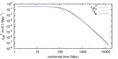
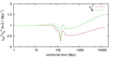
With this formulation, we can compute the adiabatic sound speed in a stable and accurate way, without needing to evaluate the time-derivative of the background pressure . When the ncdm species is no longer relativistic, its pressure perturbation defined in Eq. (2b) is an independent quantity. Since we do not have an evolution equation for , we approximate by . This approximation is sometimes as much as a factor 2 wrong as shown on Fig. 1.
We tried to use an ad hoc fitting formula for to quantify the impact of this approximation, and we found that although there was an improvement at the level of perturbations, the overall error was still at the same level. We conclude, that the error we make from this approximation is at least not dominating the total error of our approximation scheme.
3.3 Evolution equation for the shear
Given an ansatz for , we can derive a formally correct evolution equation for the shear. We follow Ma and Bertschinger, and close the system using their suggested recurrence relation for massive neutrinos222The recurrence relation in the massless limit is better motivated theoretically, since when metric perturbations vanish or satisfy a simple constraint (namely, in the Newtonian gauge). In the massive case, the formal solution involves more complicated oscillating functions with arguments going from in the massless limit to in the massive limit, as can be checked from eq. (9).. The truncation law presented in Ma and Bertschinger is valid for : in this case, all quantities are gauge-invariant. When writing the same ansatz for , we have to face the issue of the gauge dependence of . Asssuming that the truncation law holds for gauge-invariant quantities, one obtains in the synchronous gauge:
| (16) |
Throughout this subsection and the next one, one can recover Newtonian gauge equations by simply taking . We now differentiate equation (2d):
| (17) |
We can compute the right-hand side using Eq. (4c) and replace with its approximate expression from (16). After carrying out integrals over momentum, one gets:
| (18) |
where we have borrowed the notation
| (19) | ||||
| (20) |
from [10]. From the definition it is clear that and in the relativistic limit, and that and become suppressed in the non-relativistic regime compared to and . Our differential equation for differs from its Newtonian gauge counterpart in [10], because we have used the recurrence relation to truncate the hierarchy, while Shoji and Komatsu have used . The evolution equation for the shear can be further simplified by using Eq. (14), leading to:
| (21) |
3.4 Estimating quantities of higher velocity weight
One way to close the system governing the fluid approximation is to replace and by the usual quantities and multiplied by functions depending only on background quantities (in the same way that we already approximated by ). More explicitly, our aim is to write an approximation of the type , where could be any function of time going from one third in the relativistic limit to zero in the non-relativistic one. Since and are not gauge-independent, we should search for a similar approximation holding on their gauge-independent counterpart. In the synchronous gauge, such an approximation would read
| (22) |
However, we will stick to the notations of [8], who introduced a viscosity speed related to our through
| (23) |
With such assumptions, the approximate equation for the shear would read
| (24) |
Since the suppression factor which appears in Eq. (19, 20) compared to Eq. (2c, 2d) is also found in the pressure integral compared to the energy density integral, we may guess that the relative behaviour is similar, i.e. related by . This leads to a guess and which implies . However, the same logic would imply , which we have shown in Fig. 1 is not exactly true.
Let us investigate a bit how to approximate higher momenta quantities like and . If we want to approximate for instance, we may assume some functional form of described by a single (time dependent) parameter. We can make the ansatz , and then use to determine the parameter . We then find
| (25) |
The guess can be seen to be a special case of this approach having . The problem is that the value of best approximating the behavior of and other momenta is not the same in the relativistic and non-relativistic limit. In fact our testing shows that this guess sources too much during the relativistic to non-relativistic transition compared to the exact solution. Instead we got much better results by using , which avoids this excessive sourcing during the transition, while still reducing to in the relativistic limit.
For the ratio , the assumption of a -independent (i.e. ) yields , which provides satisfactory results and is adopted in the schemes described below.
We speculate that by pushing these kinds of considerations further, one could find better approximations for , and . It is also possible that another independent equation could be found, and that it would allow a better determination of .
3.5 Implementation in CLASS
For comparison, we have implemented 3 different Non-Cold Dark Matter Fluid Approximations (NCDMFA) in CLASS which differ only in their respective equation for the shear. In correspondence with the Ultra-relativistic Fluid Approximation discussed in [5], we have named the approximations MB, Hu and CLASS: in the relativistic limit, they reduce to their relativistic counterpart in [5]. In all three approximations we are using Eq. (13a) and (13b) as the first two equations with . The respective equations for the shear read
| (26a) | |||||
| (26b) | |||||
| (26c) | |||||
The second shear equation, named Hu, corresponds exactly to the prescription of Ref. [8] for approximating massive neutrinos. The first shear equation, MB, comes directly from (24) with the values of and motivated in the previous subsection. Finally, in [5], we found that removing the term leads to slightly better results for the matter power spectrum, and can be justified using an analytic approximation to the exact equations. By analogy, we also define in the massive neutrino case a CLASS approximation identical to the MB one except for the omission of this term.

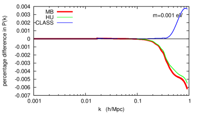

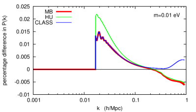
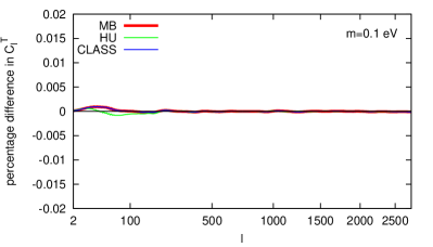
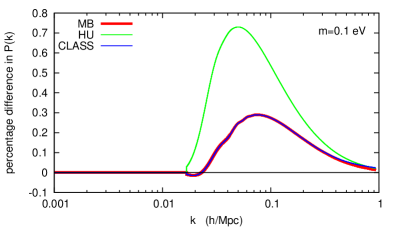
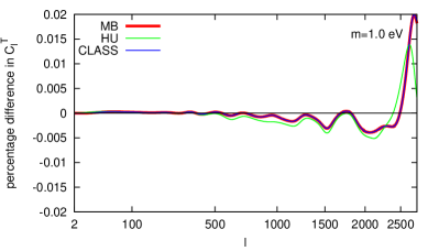
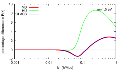
In Fig. 2 we have tested these three fluid approximations in a model with no massless neutrinos and 3 degenerate massive neutrinos. The three approximations work very well as long as the neutrinos are light and become non-relativistic after photon decoupling. Like in the massless case, the CLASS approximation is slightly better for predicting the matter power spectrum on small scales, and we set it to be the default method in the code. When the mass increases, the fluid approximation alters the CMB spectra on small angular scales (), but the error remains tiny (only 0.02% for for three species with ). The effect on the matter power spectrum is stronger: with three 1 eV neutrinos, the is wrong by 1 to 3% for . Hence, we recommend to use the fluid approximation for any value of the mass when computing CMB anisotropies, and only below a total mass of one or two eV’s when computing the matter power spectrum. However, cosmological bounds on neutrino masses strongly disfavour larger values of the total mass. This means that in most projects, CLASS users can safely use the fluid approximation for fitting both CMB and large scale structure data.
4 Standard massive neutrinos
We first illustrate our approach with the simple case of standard massive neutrinos with a Fermi-Dirac distribution. In this case, for each neutrino, the user should provide two numbers in the input file: the mass , and the relative temperature T_ncdm (the ratio of neutrino to the photon temperature). The CLASS input file explanatory.ini recommends to use the value T_ncdm=0.71599, which is “fudged” in order to provide a mass-to-density ratio eV in the non-relativistic limit. This number gives a very good approximation to the actual relic density of active neutrinos, resulting from an accurate study of neutrino decoupling [11]. However, when comparing the CLASS results with those from CAMB, we take T_ncdm=0.7133 in order to recover the mass-to-density ratio assumed in that code. Finally, if no temperature is entered, the code will default to the instantaneous decoupling value of .
4.1 Agreement with CAMB
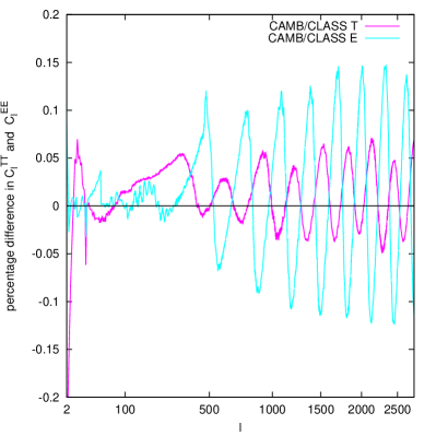
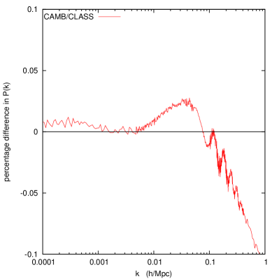
In Fig. 3, we compare the CMB and matter power spectrum from CAMB and CLASS (without the NCDM fluid approximation) for two massless and one massive neutrino with (corresponding to a mass ). We used high accuracy settings for CAMB, described in [6] under the name [CAMB:07]. For CLASS, we used the input file cl_ref.pre, which corresponds to the setting [CLASS:01] in [6] for parameters not related to NCDM; for the latter, cl_ref.pre contains the settings described in the first column of Table 1. For such settings and in absence of massive neutrinos, the two temperature spectra would agree at the 0.01% level in the range ; at the 0.02% level for polarization in the same range; and at the 0.01% level for the matter power spectrum for . With a neutrino mass close to 1 eV, we see in Fig. 3 that the discrepancy is approximately six times larger than in the massless case. However, it remains very small: even with massive neutrinos the two codes agree to better than 0.1% for the CMB and matter power spectra. This is by far sufficient for practical applications.
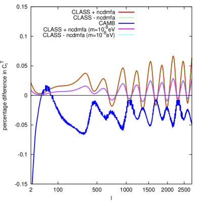
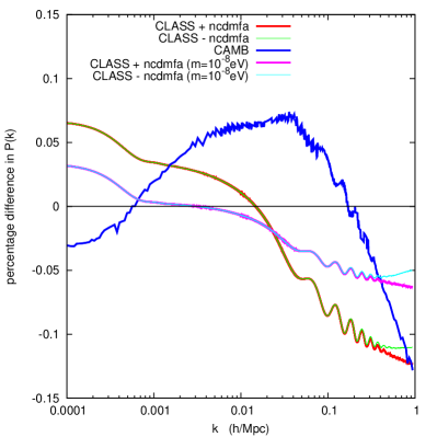
In a perfect implementation of massless and massive neutrinos in Boltzmann codes, we expect that in the relativistic limit (where is the neutrino temperature today) the spectra would tend towards those obtained with three massless species (provided that we are careful enough to keep the same number of relativistic degrees of freedom ). We performed this exercise for both codes, and the results are presented in Fig. 4. It appears that with a small enough mass, CLASS can get arbitrarily close to the fully relativistic case: with a mass of , the difference is at most of 0.03% in the ’s and 0.05% in the . This test is another way to validate the accuracy of our implementation.
4.2 Precision files
We now come to the question of defining degraded accuracy settings for computing the spectra in a fast way, while keeping the accuracy of the results under control. For such an exercise, we need to define a measure a precision. Like in [6], we will use an effective which mimics the sensitivity of a CMB experiment like Planck to temperature and E-polarisation anisotropies.
This is a time consuming exercise, which we have described in details in Sec. B of the appendix. The end result is a set of precision-files which guarantees a certain precision when used, and these files are of course available for download on the CLASS web page333http://class-code.net.
4.3 Performance
The quadrature method reveals to be extremely useful since even with five values of the momenta, we get accurate results leading to 0.2%-0.3% accuracy on the , 0.1% accuracy on the and . Traditional Boltzmann codes employ 14 momenta in order to achieve a comparable precision. In the presence of massive neutrinos, the total execution time of a Boltzmann code is dominated by the integration of the perturbation equations, which depends on the total number of perturbed variables, itself dominated by the number of massive neutrino equations. By reducing the number of momenta from 14 to 5, the quadrature method speeds up the code by more than a factor two. We find that the use of the fluid approximation leads to an additional 25% speed up for standard accuracy settings (like those in the file chi2pl1.pre). In total, for a single massive neutrino, our method speeds up the code by a factor 3. This means that instead of being 4.5 times slower in presence of one massive neutrino, CLASS only becomes 1.5 times slower. We checked these numbers with various masses and accuracy settings.
4.4 Realistic mass schemes
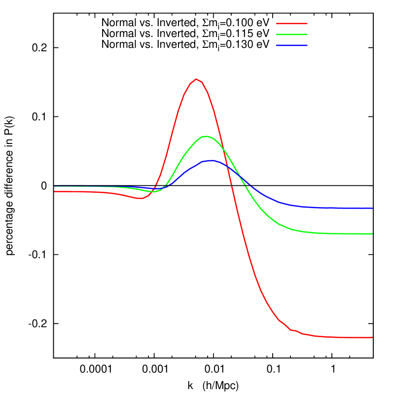
We have proved in this section that CLASS can be employed in any project requiring high-precision computations of cosmological observables in presence of massive neutrinos. It is of course perfectly suited for realistic situations with different neutrino species and masses.
To illustrate this, we display in Figure 5 the ratio of pairs of matter power spectra for models with three massive neutrinos satisfying constraints from atmospheric/solar oscillation experiments [12] (, ). Each pair of models corresponds to one normal hierarchy and one inverted hierarchy scenario, with the same total mass , equal to eV, eV or eV. The first total mass is very close to the minimum allowed value for the inverted hierarchy, eV. For each pair or models with a given :
-
•
on intermediate scales, the bump reflects the difference in the three free-streaming scales involved in the two models.
-
•
in the large limit, the two spectra are offset by 0.03% to 0.22%: it is known that in this limit, the suppression in the power spectrum induced by neutrino free-streaming depends mainly on the total mass (through the famous approximate formula), but also slightly on the mass splitting (in [13], a more accurate formula gives the suppression as a function of both the total mass and number of degenerate massive neutrinos). When increases, the two models are less different from each other (they go towards a common limit, namely the degenerate mass scenario), and the discrepancy is less pronounced.
-
•
in the small limit, the two spectra are nearly identical. The tiny difference, which increases when decreases, is due to the fact that in the inverted hierarchy model, there is a very light neutrino just finishing to complete its non-relativistic transition today. It therefore has a non-negligible pressure, which slightly affects metric perturbations on large wavelengths.
Observing the difference between these two models would be extremely challenging, although 21 cm surveys could reach enough sensitivity [14].
5 Beyond standard massive neutrinos
In this section we will illustrate the power and flexibility of the non-cold Dark Matter implementation in CLASS, by implementing different models which have already been studied elsewhere in the literature.
5.1 Massive neutrinos with large non-thermal corrections
It is plausible that some new physics can introduce non-thermal corrections to an otherwise thermal Fermi-Dirac distribution function. One might think of using CMB and large scale structure data to put bounds on such non-thermal corrections, as was described e.g. in [15]. CLASS is ideally suited for playing with such models. As a test case, we take the following distribution from [15]:
| (27) |
which is the Fermi-Dirac distribution with an added Gaussian peak in the number density. This distribution could presumably be the result of some particle suddenly decaying into neutrinos at a late time.
In practise, we only need to change the expression for in CLASS, which appears in a unique line (in the function background_ncdm_distribution()). All the rest, like density-to-mass relation and computation of the logarithmic derivative, is done automatically by the code. In particular, we do not need to change the accuracy parameters tol_ncdm and tol_ncdm_bg: the momentum sampling algorithm automatically increases the number of momenta by a significant amount, in order to keep the same precision. If this was not the case, the effect of the peak would be underestimated because of under sampling, and the parameter extraction would then likely be biased.
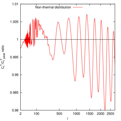
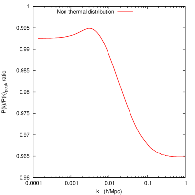
In Fig. 6, we show the CMB and matter power spectra for this model, relative to a standard model with three thermally distributed neutrinos. The two models are chosen to share exactly the same masses and the same initial number of relativistic degrees of freedom . Nevertheless, they do not have the same non-relativistic neutrino density and average neutrino momentum; in particular, non-thermal neutrinos in the decay peak become non-relativistic slightly later. This induces a combination of background and perturbation effects affecting CMB and matter power spectra in a significant way.
5.2 Warm dark matter with thermal-like distribution
There is an infinity of possible warm dark matter models, since the phase-space distribution of warm dark matter depend on the details of its production mechanism. The most widely studied model is that of non-resonantly produced warm dark matter with a rescaled Fermi-Dirac distribution, having the same temperature as that of active neutrinos. This model is implemented in the default CLASS version: when the user enters a temperature, a mass and a density (or ) for the same species, the code knows that the degeneracy parameter in front of the Fermi-Dirac distribution must be rescaled in order to match these three constraints simultaneously. The code will also ensure that the perturbations begin to be integrated when the non-cold species is still relativistic, in order to properly follow the transition to the non-relativistic regime.
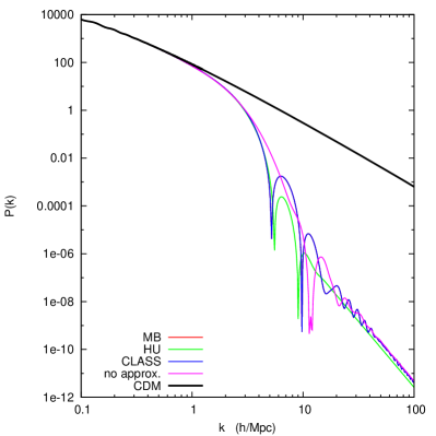
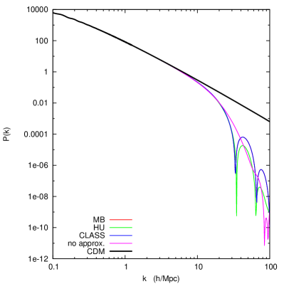
We illustrate this by running a WDM model with a mass of or and a density , with or without the fluid approximation. We compare the results with those of CDM with , in order to show the well-known suppression effect of WDM in the small-scale limit of the matter power spectrum. It appears that the fluid approximation works very well in those cases, unless one wants to resolve the details of the WDM acoustic oscillations on very small scales, first predicted in [16].
5.3 Warm dark matter with non-trivial production mechanism
Non-resonantly produced warm dark matter candidates are severely constrained by Lyman- bounds, but such bounds do not apply to other warm particles which could have been produced through more complicated mechanisms (e.g. resonant production), leading to a non-trivial, model-dependent phase-space distribution function [17]. It is not always easy to find a good analytic approximation for such a distribution; this is anyway not an issue for CLASS, since the code can read tabulated values of from an input file.
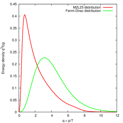
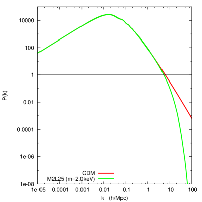
We illustrate this case by taking a particular model for resonantly produced sterile neutrinos, which distribution was computed numerically by [18] (simulating the details of sterile neutrino production and freeze-out), and stored in a file with discrete , values. Again, we only need to specify the name of this file in the CLASS input file, to enter a value for the mass and for the density , and the rest is done automatically by the code (finding the mass-density relation and the correct normalization factor for , defining the new momentum steps, deriving with a good enough accuracy). The assumed and the resulting matter power spectrum when the mass is set to is shown in Fig. 8. By eye, this spectrum seems identical to a thermal-like WDM one, but the cut-off is in fact much smoother due to an excess of low-momentum particles in this model (which behave like a small cold dark matter fraction).
6 Conclusions
A large fraction of the activity in cosmology consists in deriving bounds on particle physics in general, and on the neutrino and dark matter sector in particular. Fitting cosmological data with non-standard neutrinos or other non-cold relics require non-trivial changes in existing public Boltzmann codes. Moreover, running parameter extraction codes including massive neutrinos or more exotic non-cold relics is computationally expensive due to a significant increase in the number of differential equations to be solved numerically for each set of cosmological parameters.
The newly released Cosmic Linear Anisotropy Solving System aims at rendering this task easy and fast. The code provides a very friendly and flexible input file in which users can specify a lot of non-standard properties for the NCDM sector: masses, temperatures, chemical potentials, degeneracy parameters, etc. Moreover, the Fermi-Dirac distribution function is not hard-coded in CLASS; it is just a default choice appearing in one line of the code, which can be very easily modified. Even when a non-thermal distribution does not have a simple analytic expression, the code can be told to read it directly from a file. After reading this function, CLASS performs a series of steps in a fully automatic way: finding the mass-density relation, defining an optimal sampling in momentum space with a sophisticated but fast algorithm, and accurately computing the derivative of , needed in the perturbation equations.
In this paper, we presented the main two improvements related to the NCDM sector in CLASS: an adaptive quadrature sampling algorithm, which is useful both for the purpose of flexibility (the sampling is always adapted to any new distribution function) and speed (the code sticks to a minimum number of momenta, and hence, of perturbation equations); and a fluid approximation switched on inside the Hubble radius. We showed that the latter approximation works very well for realistic active neutrinos (with a total mass smaller than ), and for warm dark matter candidates becoming non-relativistic during radiation domination. In between these two limits, there is a range in which the accuracy of the fluid approximation is not well established, and in which the user may need to keep the approximation off, at the expense of increasing the execution time. However, the range between a few eV and few keV is usually not relevant in most realistic scenarios.
The adaptive quadrature sampling algorithm and the fluid approximation both contribute to a reduction in the total execution time of the code by a factor of three for ordinary neutrinos. This means that when one massive neutrino species is added to the CDM model, CLASS becomes 1.5 times slower instead of 4.5 times slower like other codes. Since the code is already quite fast in the the massless case, we conclude that the global speed up is significant and appreciable when fitting cosmological data.
Acknowledgments
We wish to thank Oleg Ruchayskiy for providing the phase-space distribution of the Warm Dark Matter model, Fig. 8, which gave us an opportunity to test the code in a non-standard scenario. We also wish to thank Emanuele Castorina for many useful discussions on the fluid approximation for neutrinos during his stay at CERN.
Appendix A Optimal momentum sampling
We define a quadrature rule on to be a set of weights and a set of nodes , such that
| (28) |
Note that the distribution function itself has been absorbed into the weights. The optimal quadrature rule will depend on both the distribution and the accuracy requirement tol_ncdm, but the specific method used for obtaining the rule is decoupled from the rest of the code; the output is just two lists of points, and . CLASS tries up to three different methods for obtaining the most optimal quadrature rule, each with its own strength and weaknesses. These are Gauss-Laguerre quadrature, adaptive Gauss-Kronrod quadrature and a combined scheme. We will now discuss each of them.
A.1 Gauss-Laguerre quadrature
Most of the time, the distribution function will be close to a Fermi-Dirac distribution, and the integrand is exponentially decaying with . The Gauss-Laguerre quadrature formula is well suited for exponentially decaying integrands on the interval , so this is an obvious choice. The rule is [19]
| (29) |
where the nodes are the roots of , the Laguerre polynomial of degree and the weights can be calculated from the formula
| (30) |
If we put we obtain the rule
| (31) |
This rule will be very effective when the ratio is well described by a polynomial, but it will converge very slowly if this is not the case.
A.2 Adaptive sampling
When an integrand has structure on scales smaller than the integration interval, an adaptive integration scheme is often the best choice, since it will subdivide the interval until it resolves the structure and reach the required accuracy. We will use the 15 point Gauss-Kronrod quadrature formula as a basis for our adaptive integrator; 7 of the 15 points can be used to obtain a Gauss quadrature estimate of the integral, and the error estimate on the 15 point formula is then [20].
The Gauss-Kronrod formula is defined on the open interval , but it can be rescaled to work on an arbitrary open interval . We transform the indefinite integral into a definite integral by the substitution :
| (32) |
This integral can then be solved by the adaptive integrator. If the tolerance requirement is not met using the first 15 points, the interval is divided in two and the quadrature method is called recursively on each subinterval.
This method is very efficient when the integrand is smooth. For practical purposes, this will be the case unless the phase-space distribution is read from a file with sparse sampling: in this case, the code must interpolate or extrapolate the file values in order to cover the whole momentum range, and the next method may be more efficient.
A.3 Integration over tabulated distributions
If some distribution function is not known analytically, but only on a finitely sampled grid on , we have to interpolate the distribution function within the interval, and we have to extrapolate the behaviour outside the interval. Inside the interval we use a spline interpolation, while we assume close to zero. For the tail, we assume the form . Requiring the function and its first derivative to be continuous at the point leads to the following equations for and :
| (33) | ||||
| (34) |
In the combined scheme we use the 4 point Gauss-Legendre method on the interval , adaptive Gauss-Kronrod quadrature on and the 6 point Gauss-Laguerre rule on the tail 444This version of the rule is obtained by a simple substitution.. This scheme works well when the integrand is interpolated from tabulated points.
A.4 Implementation in CLASS
When CLASS initialises the background structure, it will find optimal momentum samplings for each of the species. More specifically, we start by computing the integral of the distribution function multiplied by the test function at high accuracy, which gives a reference value which can be used for comparison. It also creates a binary tree of refinements, from which we can extract integrals at various levels, where level 1 is the best estimate. We choose the highest possible level which results in an error which is less than the input tolerance, and we extract the nodes and weights from that level.
The code will now search for the lowest number of nodes required for computing the integral with the desired accuracy using Gauss-Laguerre quadrature. The most efficient method, the method using the lowest number of points, is then chosen. For a distribution not departing too much from a Fermi-Dirac one, this will usually be Gauss-Laguerre quadrature.
The scheme suggested here has the benefit, that there is just one tolerance parameter directly related to how well the integral is approximated, independently of the distribution function. However, for this to be exactly true, we require the test function to be a sufficiently realistic representation of for and for the perturbations555The energy behaves like in the relativistic limit and like a constant in the non-relativistic limit, so there is an intermediate range where it is not completely described by a polynomial of finite order. However, we do not think this error is a dominant one.. We have tried different test functions, but in the end we found the polynomial to be adequate. The coefficients were chosen such that
| (35) |
When the phase-space distribution function is passed in the form of a file with tabulated values, the code compares the three previous methods (still with a common tolerance parameter) and keeps the best one, which is usually the third one in the case of a poor sampling of the function, or one of the other two in the opposite case.
Appendix B ncdm accuracy settings
Taking the runs with accuracy settings cl_ref.pre as a reference, we decrease the precision for each parameter while keeping the roughly below a given limit, chosen to be either 0.1 or 1. This exercise was already performed in [6] for all parameters not related to NCDM, leading to the definition of two precision files chi2pl0.1.pre and chi2pl1.pre which are available on the CLASS web site. Here, we only need to set the NCDM precision parameters in these two files to correct values. Our results are listed in Table 1, in the second and third columns. They take advantage of the fluid approximation, and use an extremely small number of momenta (8 or 5 only). We checked that these settings provide the correct order of magnitude for within a wide range of neutrino masses, at least up to 2 eV. This is shown in Table 2 for the two cases chi2pl0.1.pre and chi2pl1.pre, as well as for the case chi2pl1.pre with the fluid approximation removed. Around eV, the error induced by the fluid approximation starts increasing significantly: when exploring this region, the user should either turn off the approximation, or increase the value of the trigger. Given current limits on active neutrino masses, the interesting mass range to explore is below 2 eV, and in most projects, the CLASS users can safely employ the default settings of chi2pl0.1.pre and chi2pl1.pre including the fluid approximation.
These settings are optimised for fitting the CMB spectra only. For the matter power spectra, the files chi2pl0.1.pre and chi2pl1.pre produce an error of the order of a few per cents in the range (for any neutrino mass and with/without the fluid approximation). In order to get accurate matter power spectra, it is better to employ the settings cl_permille.pre, cl_2permille.pre, cl_3permille.pre, which lead to a precision of 0.1%, 0.2% or 0.3% for in the range , even in the presence of neutrino masses. In these files, we fixed the fluid approximation trigger to a rather larger value in order to get a precision of one permille for the matter power spectrum for and eV, or a bit worse for mildly non-linear scales . The power spectrum accuracy with such settings is indicated in Table 3 for various values of the mass.
| cl_ref.pre | chi2pl0.1.pre | chi2pl1.pre | |
| tol_ncdm_bg | |||
| tol_ncdm | |||
| l_max_ncdm | 51 | 16 | 12 |
| fluid approximation | none | ncdmfa_class | ncdmfa_class |
| trigger | – | 30 | 16 |
| number of (back.) | 28 | 11 | 11 |
| number of (pert.) | 28 | 8 | 5 |
| number of neutrino equations | 1428 | 1363 | 653 |
| mass (eV) | chi2pl0.1.pre | chi2pl1.pre | same without approx. |
|---|---|---|---|
| 0.087 | 0.94 | 0.90 | |
| 0.087 | 0.93 | 0.92 | |
| 0.1 | 0.092 | 0.90 | 0.92 |
| 1 | 0.083 | 0.96 | 0.82 |
| 2 | 0.157 | 1.10 | 0.93 |
| mass (eV) | ||
|---|---|---|
| 0.04% | 0.12% | |
| 0.04% | 0.12% | |
| 0.1 | 0.05% | 0.12% |
| 1 | 0.06% | 0.8% |
| 2 | 0.2% | 1.5% |
References
- [1] U. Seljak and M. Zaldarriaga, “A Line of sight integration approach to cosmic microwave background anisotropies,” Astrophys.J. 469 (1996) 437–444, arXiv:astro-ph/9603033 [astro-ph].
- [2] A. Lewis, A. Challinor, and A. Lasenby, “Efficient computation of CMB anisotropies in closed FRW models,” Astrophys.J. 538 (2000) 473–476, arXiv:astro-ph/9911177 [astro-ph].
- [3] M. Doran, “Cmbeasy:: an object oriented code for the cosmic microwave background,” JCAP 0510 (2005) 011, arXiv:astro-ph/0302138 [astro-ph].
- [4] J. Lesgourgues, “The Cosmic Linear Anisotropy Solving System (CLASS) I: Overview,” arXiv:1104.2932 [astro-ph.IM].
- [5] D. Blas, J. Lesgourgues, and T. Tram, “The Cosmic Linear Anisotropy Solving System (CLASS) II: Approximation schemes,” arXiv:1104.2933 [astro-ph.CO].
- [6] J. Lesgourgues, “The Cosmic Linear Anisotropy Solving System (CLASS) III: Comparision with CAMB for LambdaCDM,” arXiv:1104.2934 [astro-ph.CO].
- [7] C.-P. Ma and E. Bertschinger, “Cosmological perturbation theory in the synchronous and conformal Newtonian gauges,” Astrophys.J. 455 (1995) 7–25, arXiv:astro-ph/9506072 [astro-ph].
- [8] W. Hu, “Structure formation with generalized dark matter,” Astrophys.J. 506 (1998) 485–494, arXiv:astro-ph/9801234 [astro-ph].
- [9] A. Lewis and A. Challinor, “Evolution of cosmological dark matter perturbations,” Phys.Rev. D66 (2002) 023531, arXiv:astro-ph/0203507 [astro-ph].
- [10] M. Shoji and E. Komatsu, “Massive Neutrinos in Cosmology: Analytic Solutions and Fluid Approximation,” Phys.Rev. D81 (2010) 123516, arXiv:1003.0942 [astro-ph.CO].
- [11] G. Mangano, G. Miele, S. Pastor, T. Pinto, O. Pisanti, et al., “Relic neutrino decoupling including flavor oscillations,” Nucl.Phys. B729 (2005) 221–234, arXiv:hep-ph/0506164 [hep-ph].
- [12] Particle Data Group Collaboration, K. Nakamura et al., “Review of particle physics,” J.Phys.G G37 (2010) 075021.
- [13] J. Lesgourgues and S. Pastor, “Massive neutrinos and cosmology,” Phys.Rept. 429 (2006) 307–379, arXiv:astro-ph/0603494 [astro-ph].
- [14] J. R. Pritchard and E. Pierpaoli, “Neutrino mass from cosmological 21 cm observations,” Nucl.Phys.Proc.Suppl. 188 (2009) 31–33.
- [15] A. Cuoco, J. Lesgourgues, G. Mangano, and S. Pastor, “Do observations prove that cosmological neutrinos are thermally distributed?,” Phys.Rev. D71 (2005) 123501, arXiv:astro-ph/0502465 [astro-ph].
- [16] D. Boyanovsky and J. Wu, “Small scale aspects of warm dark matter : power spectra and acoustic oscillations,” Phys.Rev. D83 (2011) 043524, arXiv:1008.0992 [astro-ph.CO].
- [17] A. Boyarsky, J. Lesgourgues, O. Ruchayskiy, and M. Viel, “Realistic sterile neutrino dark matter with keV mass does not contradict cosmological bounds,” Phys.Rev.Lett. 102 (2009) 201304, arXiv:0812.3256 [hep-ph].
- [18] M. Laine and M. Shaposhnikov, “Sterile neutrino dark matter as a consequence of nuMSM-induced lepton asymmetry,” JCAP 0806 (2008) 031, arXiv:0804.4543 [hep-ph].
- [19] M. Abramowitz and I. A. Stegun, Handbook of Mathematical Functions with Formulas, Graphs, and Mathematical Tables. Dover Publications, New York, 1964.
- [20] D. Kahaner, C. Moler, and S. Nash, Numerical Methods and Software. Prentice-Hall series in computational mathematics. 1989.