The Cosmic Linear Anisotropy Solving System
(CLASS) II: Approximation schemes
Abstract:
Boltzmann codes are used extensively by several groups for constraining cosmological parameters with Cosmic Microwave Background and Large Scale Structure data. This activity is computationally expensive, since a typical project requires from to Boltzmann code executions. The newly released code CLASS (Cosmic Linear Anisotropy Solving System) incorporates improved approximation schemes leading to a simultaneous gain in speed and precision. We describe here the three approximations used by CLASS for basic CDM models, namely: a baryon-photon tight-coupling approximation which can be set to first order, second order or to a compromise between the two; an ultra-relativistic fluid approximation which had not been implemented in public distributions before; and finally a radiation streaming approximation taking reionisation into account.
1 Introduction
Boltzmann codes have experienced considerable improvements in terms of precision and speed with respect to the pioneering COSMICS package [1]. In each new public code (CMBFAST [2], CAMB [3], CMBEASY [4]), several sophisticated optimisation methods and approximation schemes have been introduced. Efforts on this side keeps being justified for two reasons. On the one hand, we need to fit data with higher and higher precision. For instance, the analysis of Planck data requires much more accurate theoretical predictions than for WMAP [5]. On the other hand, a growing number of cosmologists are interested in fitting cosmological data with several extensions of the minimal cosmological model, in order to probe new physics. This requires running parameter extraction algorithms on computer clusters, often involving or Boltzmann code executions (for each new model or new combination of data sets). Hence, any way to speed up Boltzmann codes without loosing precision is useful.
In front of such needs, a new code, the Cosmic Linear Anisotropy Solving System (CLASS) [6], has just been released111available at http://class-code.net. The goal of this project is not just to improve speed and precision, but also to provide a flexible and user-friendly code that can be easily generalized to non-minimal cosmological models. In this paper, we do not discuss flexibility issues and only concentrate on the improved approximation schemes used by CLASS, in the strict context of minimal CDM cosmology. Extensions requiring extra approximations may be introduced and discussed case by case in the future. In a companion paper [7], we already discuss the approximation specific to massive neutrinos and non-cold dark matter relics. A comparison between the power spectra obtained by CAMB and CLASS for the minimal CDM model, as well as estimates of the relative speed of the two codes, is presented in [8].
The next three sections describe: a baryon-photon tight-coupling approximation which can be set to first order, second order or to a compromise between the two (Sec. 2); an ultra-relativistic fluid approximation which had not been implemented in public distributions of Boltzmann codes before (Sec. 3); and a radiation streaming approximation consistently including reionisation (Sec. 4). Appendix A describes the stiff integrator which can be used by CLASS as an alternative to the Runge-Kutta integrator: without this integrator, it would have been essentially impossible to launch test runs with no approximation schemes, to evaluate the error induced by these schemes; moreover, this integrator gives better performances even in the presence of approximations, and is set to be the default integrator in CLASS. We summarize our full approximation landscape in Sec. 5.
Note that throughout this paper, when discussing CAMB and CLASS, we refer to the versions available at the time of preparing this manuscript, i.e. the January 2011 version of CAMB and v1.1 of CLASS.
2 Tight Coupling Approximation (TCA)
Before recombination, when the opacity is very large, the equations governing the tightly coupled baryon-photon fluid form a stiff system. Indeed, the opacity defines a conformal time scale of interaction considerably smaller than that on which most of the modes actually evolve, namely for super-Hubble scales and for sub-Hubble scales (see Fig. 1). Standard integrators like Runge-Kutta algorithms would be very inefficient in solving such a system. This motivated Peebles & Yu to introduce a simplified system of differential equations valid in the regime of small and (tight coupling approximation or TCA) [9]. The overall idea is that quantities which are vanishingly small in the limit are solved perturbatively in , and these analytical expressions are used in the numerical code solving the remaining differential equations of the system.
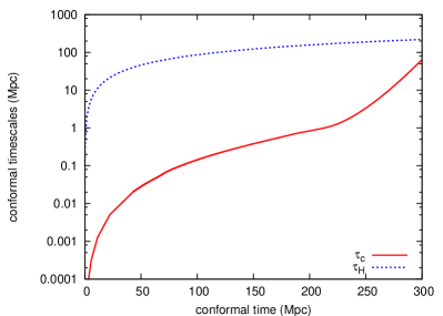
The CLASS user can choose between two integrators for the system of linear perturbations. One of them (ndf15, see Appendix A) is optimised for stiff equations, and shows good performances even in the tight coupling regime. However, by reducing drastically the number of equations to integrate, any TCA scheme leads to a speed up even in presence of such an integrator.
Tight coupling equations have already been derived and improved by many authors after Peebles & Yu’s seminal paper. For instance, the TCA formulas presented in Ma & Bertschinger [10] are derived to first order in (omitting some polarisation terms which contribute to the photon shear at this order). Lewis et al. implemented the full first-order solution in CAMB [3], also relaxing Ma & Bertschinger’s assumption that . Doran implemented some improved formulas in CMBEASY which are valid in the Newtonian gauge, and include a few contributions beyond order one [11].
As we will see below, the first-order TCA formulas provide poor approximations to the baryon-photon differential energy flux and to the photon shear at large times. This is not much of a problem if one switches to the exact222 It should be intended that throughout this section, the word “exact” is intended in the sense “without using the TCA”. Obviously, our equations are never exact since they rely on a number of common and well-justified approximations, e.g.: linear perturbations, pressureless CDM, approximate expression for photon-baryon coupling, baryon pressure neglected in several equations, etc. equations early enough. However, a better scheme would allow to switch off the TCA later, and to save a lot of integration time without loosing precision.
Here, we will derive the full second-order TCA formulas in the synchronous gauge. While this work was in preparation, Cyr-Racine and Sigurdson published a paper on exactly the same topic [12]. We will show that the numerical results from our approach coincide with those of [12]. Another recent paper discussing the TCA beyond first order and its implementation in second order cosmological perturbation theory is [14]: this work actually proposes a systematic way to compute high-order corrections in a given model and at any order333 As pointed out by the author of [14], this method can be implemented numerically provided that the code computing the evolution of thermodynamical variables outputs fully continuous and derivable functions of time, which is precisely the case with the CLASS version of RECFAST..
2.1 Full equations
In the following we will adopt the notation of Ma & Bertschinger [10]. The baryon perturbations will be characterized by the energy density contrast and the divergence of the fluid energy flux . These quantities satisfy the equations444We will work in Fourier space and stick to the synchronous gauge in conformal time, which we will denote by . We use the prime to denote derivative with respect to conformal time.
| (1a) | |||
| (1b) | |||
with , where is the scale factor, and we have defined and . The quantity represents the divergence of the energy flux of the photons () in the frame comoving with the baryons. Its time-derivative is often referred to as the “baryon-photon slip”. The fields and represent the metric perturbations. As explained in [10], the baryon pressure perturbation can be safely neglected in the continuity equation, but its Laplacian should be kept in the Euler equation (giving raise to the term ) since it affects the evolution of very small wavelengths, smaller than the baryon Jeans length. In [10] and many other references, the baryon sound speed is identified to the adiabatic sound speed
| (2) |
where the evolution of the proton temperature is given by
| (3) |
and is the mean molecular weight. This approximation has been proved to be inaccurate in refs. [15, 16], but the difference is only important for computing the matter power spectrum for Mpc-1. The current version of CLASS (v1.1) and CAMB (from January 2011) still relies on the approximation, while future versions of both codes are likely to switch to the actual sound speed calculation, as in the CAMB_source555http://camb.info/sources/ code. This issue is irrelevant for the results of this paper, which do not involve very large wavelengths. All numerical results below have been obtained using instead of , but our formulas can adequately describe the large range, provided that a correct sound speed calculation is performed.
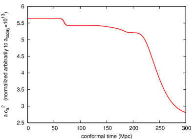
Like the adiabatic sound speed, the actual baryon sound speed is expected to decrease approximately as , except during helium and hydrogen recombination (see Fig. 1).
The characterization of the photon distribution requires the determination of its different multipoles , , and for . These satisfy the recursive Boltzmann equations (Eqs. (63) in [10]):
| (4a) | |||
| (4b) | |||
| (4c) | |||
| (4d) | |||
| (4e) | |||
where we remind the reader that . Finally, the previous hierarchical equations are truncated at some following equation (65) in [10],
| (5) |
2.2 TCA equations
From Eqs. (1) and (4) one sees that the different time scales in the problem are , and the time scale of cosmological evolution . As we will show explicitly in the next section, it is possible to find a solution (, ) for the baryon-photon slip and the photon shear in terms of , , and , which is valid to any desired order in the small parameter . The knowledge of this solution helps to reduce the full system of equations (1) and (4) to just four of them for the low multipoles of the distributions. More concretely, one may use Eq. (1a) for , and Eq. (4a) to determine ; the energy fluxes are characterized by the linear combination of Eqs. (1b) and (4b) in which the coupling term vanishes:
| (6) |
and finally . As desired, this scheme allows us to get rid of any coefficient666The scale appears now as a small perturbation. in . For practical reasons it is customary to combine linearly the last two equations in order to eliminate and get an expression for only; then can be found from equation (6). In summary, once and are known the goal is to solve the closed system formed by the four equations (1a), (4a), and
| (7a) | |||||
| (7b) | |||||
2.3 Perturbative expansion
The aim of this section is to find expressions for and valid at the order in (the zero order is trivial: both species behave as a single perfect fluid, so that and all multipoles of the photons beyond and vanish; the first order can be found in [10]). We first multiply equations (4b) and (1b) by :
| (8a) | |||||
| (8b) | |||||
To obtain a differential equation for we can combine the above two equations into
| (9) |
This equation involves the photon shear, given by the following equation (see (4c)):
| (10) |
Until now, all these equations are exact. In the limit of interest, both of them can be schematically written as777This is immediate for (9). For (10) if follows from (4), and we will explicitly verify it shortly.
| (11) |
where is a small parameter. In our case, can be chosen to be , the opacity at an arbitrary time around which the expansion is performed888In fact, the small dimensionless parameters will be and , with evaluated around the same time as .. The perturbative solution is given by
| (12) |
Notice that for functions and with smooth time variations on the scale , the previous is a perfectly well defined solution. Finally, the most general solution is found by adding to the previous particular solutions the solution of the homogeneous equation
| (13) |
Note that in our case is always positive, which is enough to make this part of the solution suppressed very fast. Hence, the relevant solution is given by Eq. (12), which, after absorbing the small parameter in the function , reads:
| (14) |
In terms of these functions, the powers of and its derivatives represent the different orders of the approximation.
2.4 Second-order approximation
Using the previous expansion in Eq. (9), the baryon-photon relative velocity reads at order two:
| (15) |
with
| (16) |
We still need to differentiate this equation in order to get a similar approximation for the slip:
| (17) |
There are several ways to organise and simplify the final result. In order to write the first-order term in the same form as in the rest of the literature, we need to express in a very peculiar way:
Here we defined : this quantity would vanish if the approximation were valid at all times. In the second line, we used Eq. (1b), while in the third line we used (4b): so these expressions for are all exact.
The first-order approximation for is obtained by replacing the first occurrence of in Eq. (17) with the last expression of (2.4), in which we neglect the terms and which represent contributions of higher order. The final result is:
| (19) |
Note that in the previous expression we used the exact relation .
For the second-order expression for the slip, we go back to Eq. (17). We replace the first occurrence of by the full expression (2.4), assuming that and have been replaced by their first-order approximation. Finally, we replace , and in the last three terms by their zeroth-order approximation. The final result can be written in a compact form:
| (20) | |||||
This formula requires an expression for the shear valid at order one. However, to solve equations (1b, 4b) consistently to second order, we need the expression for the shear at the corresponding order. This can be achieved using (10). To solve this equation let us first note that the polarisation multipoles obey (cf. (4))
| (21) |
from which we see that, at first order in , . Thus, it is consistent to consider these multipoles as , and write the second order solution to (10) following (14) as
| (22) |
where we used the fact that . Indeed, the high photon multipoles obey at leading order (cf. (4d))
The final step involves an evaluation of (21). Again, from (4), one finds that
This allows us to find the perturbative solution to (21)
| (23) |
From the previous expression and (22) we find
| (24) |
which implies
| (25) |
Finally, the shear at second order is found from (22) to be
| (26) |
The last missing items are the zero-order expressions for , and appearing in equation (20). Noticing that equation (7a) implies
we can write these last terms as
| (28a) | |||||
| (28b) | |||||
| (28c) | |||||
The derivation given in [12] follows different steps, but since it is still a second-order TCA, the results should be identical under the approximation used in [12], at least up to terms of order three or higher. For the shear, our expressions are indeed exactly identical. For the slip, there are so many ways to write the result and so many terms involved that the comparison is not trivial. However, by coding the two formulas in CLASS and comparing the evolution of in the two cases, we found that the two expressions agree very well, since numerically the difference appears to be at most of order .
2.5 Implementation of various schemes in CLASS
We implemented various TCA schemes in CLASS, which can be chosen by setting the flag tight_coupling_approximation to different values. We always start integrating the wavenumbers very deep inside the tightly-coupled regime. Hence, in contrast to [12], we do not need to include terms in in the initial conditions. We always use the set of equations (1a), (4a), (7a), (7b) with different expressions for the slip and the shear :
- 1.
- 2.
- 3.
-
4.
second-order expressions from [12] when the flag is set to second_order_CRS.
- 5.
-
6.
finally, second-order expression for the shear, but a reduced expression for the slip, involving only the leading order-two terms:
(29) This option is taken when the flag is set to compromise_CLASS, and is chosen to be the default option in CLASS. Notice that the last scheme does not have a term , which is advantageous from the computational point of view999In order to compute one should use one more Einstein equation that in the standard case, and compute the component of the stress-energy tensor, i.e. the pressure perturbation for all species..
To justify the compromise scheme, notice that it encapsulates the leading order in (28) for subhorizon modes (note that has an extra momentum dependence with respect to the other perturbations, and each time derivative adds one more power of in this regime). Thus, from Eq. (20) we learn that Eq. (29) implements the leading second order correction for the modes with a big comoving momentum. It is precisely for these modes that the first order approximation fails first, which explains the success of the compromise scheme. To check that the approximation is indeed correct, we implemented this scheme for several modes assuming CDM. As illustrated in the next subsection, this scheme is nearly as good as the full second-order one, being at the same time much more compact and requiring many less floating point operations.
2.6 Comparison at the level of perturbations
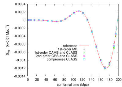
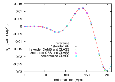
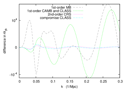
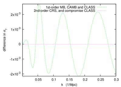
In Fig. 2, we compare these different approximations for a fixed wave number (chosen to be ), and in Fig. 3 for a fixed conformal time (chosen to be the time when the TCA is switched off in the previous example).
Scrutinising first the various first-order schemes, we see a significant difference at late time between the first two (MB and CAMB), showing that is a bad approximation. However, there is no sizable difference between the second one (CAMB) and the third one (CLASS) in which the approximation is relaxed. We reach the same conclusion when comparing second-order schemes with or without the same approximation. This is not a surprise, since we are only considering scales larger than the baryonic Jeans length at any time. When studying very small wavelengths, the CLASS user is free to choose one of the TCA schemes where the full evolution of is automatically taken into account (namely, first_order_CLASS or second_order_CLASS), but as mentioned before, in this limit, an accurate sound speed computation should also be implemented in order to relax the approximation.
Figs. 2 and 3 show that all first-order schemes provide poor approximations for the slip and the shear near the end of the tightly coupled regime, and hence, inaccurate initial conditions at the time at which the full equations are turned on. As expected, second-order schemes work much better. We find a very good agreement between second_order_CRS and second_order_CLASS: this validates both the results of [12] and our results. The residual difference is likely due to the fact that our two independent derivations lead to expressions in which some higher-order terms (of order ) appear in different ways.
These two schemes also agree to a very good extent with compromise_CLASS, which is much more straightforward to code, and computes the baryon-photon slip with approximately ten times less operations. In particular, with this scheme, the code does not even need to compute the quantities , and , which are not so obvious to obtain with few operations and good accuracy. Hence, this method is set to be the default TCA in CLASS.
2.7 Comparison at the level of temperature/polarisation spectra
First, let us specify which precision parameters in CLASS govern the evolution of perturbations in the early universe and the TCA switching time:
-
•
two parameters define the time at which initial conditions are imposed during the tightly-coupled stage. Each wave-number starts being integrated (with one of the TCA schemes) as soon as one of the two conditions
or
is fulfilled. The second condition means that at initial time, wavelengths should be sufficiently far outside the Hubble scale; the first condition, which over-seeds the second one for the smallest wave numbers, means that the initial time should not be too close to recombination.
-
•
two parameters define the time at which the TCA is turned off for each wave number. This happens when one of the two conditions
or
is fulfilled. CLASS imposes that the TCA switching time should always be chosen after the initial time, which means that the four parameters above should satisfy simple inequalities.
-
•
one parameter defines the time (common to all wave numbers) at which the source functions (leading to the computation of temperature and polarisation ’s) start being sampled and stored. This happens when the condition
is satisfied. This time can eventually be chosen during the tight-coupling regime for the smallest wave numbers.
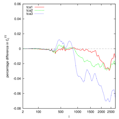
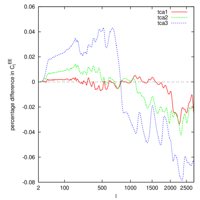
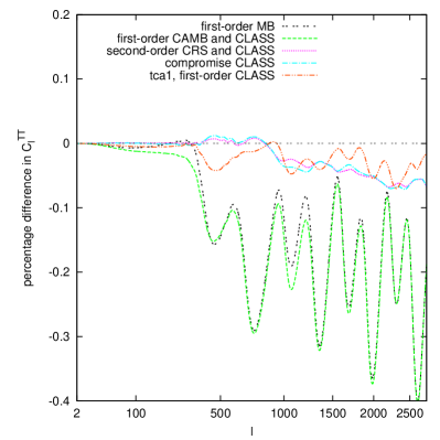
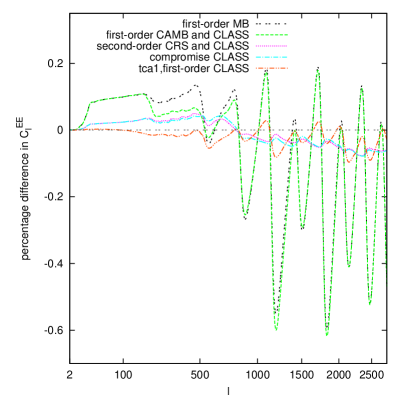
In order to show the impact of these parameters, we take the set of precision parameters defined in the file cl_permille.pre of the CLASS public distribution, which corresponds to an accuracy of at least 0.1% on each temperature and polarisation , and uses the compromise_CLASS scheme. We then vary the two trigger parameters mentioned above, as described in Table 1. The first setting, called no-tca, corresponds to switching off the tight coupling approximation immediately after setting the initial conditions, so that no TCA is ever used. This leads to reference temperature/polarisation spectra with respect to which all the other results of this section are compared. The settings called tca1, tca2 and tca3 introduce from 0.02% to 0.08% of error with respect to the no-tca case, as illustrated in Fig. 4.
In Fig. 5, we stick to the precision setting tca3 and compare the different TCA schemes. The first_order_CAMB and first_order_CLASS results are indistighuishable, confirming the fact that the approximation is sufficient in practice. Our second-order results and those derived from [12] are also in perfect agreement. As expected, the results from the compromise_CLASS scheme are essentially as good as the full second-order results, while the first-order results are roughly ten times less accurate. We also show on this plot the error produced by the first_order_CLASS scheme with tca1 precision settings, which is similar to that produced by the compromise_CLASS scheme with tca3 precision settings. Hence, in order to estimate the usefulness of going beyond the first order TCA, we can compare the performances of the code in these two cases.
In Table 2, we compare running times in the no-tca case and in the previous two cases, using either the Runge-Kutta or ndf15 integrator. The timings displayed here correspond to the number of seconds spent by our computer in the perturbation module of CLASS, in a non-parallel execution. The ndf15 integrator is always better, by a huge amount in the no-tca case, or by 20 to 30% in the other cases. Being unaffected by the issue of integrating a stiff system, the ndf15 integrator is not very sensitive to the choice of TCA scheme, with only a 3% speed up when using the compromise scheme instead of first-order schemes. The Runge-Kutta integrator is more sensitive, with a 9% speed-up for the compromise scheme.
We conclude that CLASS benefits much more from the implementation of our stiff integrator than from going beyond the first-order TCA. For some particular models, the user may wish to stick to the Runge-Kutta integrator, in which case the compromise_CLASS scheme leads to a sizable speed up.
| no-tca | tca1 | tca2 | tca3 | |
|---|---|---|---|---|
| tight_coupling_trigger_tau_c_over_tau_h | ||||
| tight_coupling_trigger_tau_c_over_tau_k |
| precision | no-tca | tca1 | tca3 |
|---|---|---|---|
| TCA scheme | (irrelevant) | first_order_class | compromise_class |
| rk | 1069s | 19.4s | 17.8s |
| ndf15 | 16s | 14.9s | 14.6s |
3 Ultra-relativistic Fluid Approximation (UFA)
All massless neutrinos and ultra-relativistic relics can be treated as a single species, labeled as “ur” in CLASS. The code assumes that these species are fully decoupled. Hence, they just free-stream within a given gravitational potential, and can be followed with the collisionless Boltzmann equation expanded in harmonic space and integrated over momentum [10]. The solution can be formally written as the sum of spherical Bessel functions (exhibiting damped oscillations for ), plus a particular solution of the inhomogeneous equations sourced by metric fluctuations. The fact that one part of the solution has an analytical expression cannot be directly implemented in the code, because the total perturbations , and back-react on the metric perturbations through Einstein equations, and affect the source terms in the Boltzmann equation. We will use this decomposition only as a guideline for deriving accurate approximation schemes.
3.1 Truncation of the Boltzmann hierarchy
Since the ur species couple only gravitationally to other species, we are only interested in tracking , and . Higher multipoles must still be included since they couple with the lower ones, but in all efficient Boltzmann codes, the hierarchy is truncated at some low multipole value . CMBFAST, CAMB, CMBEASY and CLASS all use the truncation scheme proposed in Ma & Bertschinger (Eq. (51) of [10]) which is designed to minimize artificial reflection of power from back to lower multipoles. Still, this truncation is not perfect, and a significant amount of unphysical reflection cannot be avoided for times beyond . This implies that in order to compute an accurate CMB spectrum, should be at least of the order of 30. The computation of the matter power spectrum on small scales, up to some wavenumber , is more problematic: one should further increase proportionally to in order to get converging results.
3.2 Sub-Hubble fluid approximation
The Ultra-relativistic Fluid Approximation (UFA) implemented in CLASS is based on the idea that for a given wavenumber, should not necessarily be fixed throughout the whole time evolution. The code considers two regimes: wavelengths larger or comparable to the Hubble radius, and wavelengths much smaller than the Hubble radius. The transition between the two regime occurs for each when the product (equal to and coinciding with during radiation domination) reaches some threshold value that we call here . Typically, is chosen in the range from to , depending on the required precision. The full name of this parameter in the code is ur_fluid_trigger_tau_over_tau_k. In the first regime , the Boltzmann hierarchy can be truncated at some which can be chosen to be rather small: it is enough to take to , since multipoles with are negligible (according to the spherical Bessel function approximation). In the second regime , the code still follows the three variables , and , which are sourced by metric perturbations. But multipoles in the range are suppressed, leading to an effective decoupling between the first three multipoles and the highest ones. Hence it is natural to lower down to two in this regime. Ultra-relativistic neutrinos are then described by a reduced system of equations for , and , i.e. by fluid equations (of course, this fluid is not assumed to be perfect, since it has anisotropic pressure). In summary, the UFA approximation consists in lowering from a value close to down to deep inside the Hubble radius, at the time when . Such a scheme offers many advantages:
-
1.
When computing the matter power spectrum, the number of ur equations to integrate before the approximation is switched on does not need to be scaled linearly with the highest wave number .
-
2.
The number of ur equations reduces to in the whole region of space fulfilling the condition ; this is precisely the region in which the computation would be time-consuming, since ur perturbations oscillate inside the Hubble radius.
-
3.
The UFA completely avoids the issue of power reflecting at some large , which would otherwise affect the evolution of low multipoles periodically due to some spurious wave travelling back and forth between and . (This behaviour is clearly seen in Fig. 6).
The fluid approximation could in principle be used until present time, but the code allows a more aggressive approximation, the Radiation Streaming Approximation, to take over from the UFA after photon decoupling. This new approximation is discussed in the next section. Hence, the UFA is essentially a way to save computing time during radiation domination and at the beginning of matter domination.
3.3 Fluid equations
We need to find a closed system for the evolution of , and , valid deep inside the Hubble radius. The full system of equations in the synchronous gauge (Eq. (49) in [10]) reads:
| (30a) | |||
| (30b) | |||
| (30c) | |||
| (30d) | |||
In Appendix B, we use the formal solution of these equations in order to derive an exact integral relation between , , and metric perturbations. We then find an approximate but more practical form of this relation valid inside the Hubble radius, at leading order in an expansion in metric perturbation derivatives (, ) and in powers of :
| (31) |
Since metric perturbation only evolve over a Hubble time scale inside the Hubble radius, we expect this expansion to converge, and we will see below that the above relation is indeed accurate enough for our purpose. In the default version of CLASS, this equation is used for closing the system of equations when the UFA is switched on. This method corresponds to the setting ufa_method = ufa_class in the code’s precision parameter structure.
3.4 Alternative schemes
Some nearly equivalent schemes can be justified in slightly different ways. Truncating the Boltzmann equations at with the usual truncation scheme of Ma & Bertschinger gives:
| (32) |
This truncation scheme is based entirely on the assumption that . So, the reason for the difference between eq. (31) and (32) is that (31) is based on the full formal solution, including the leading order contribution to the part sourced by the metric, while (32) is based only on the solution of the homogeneous equation. Equation (32) is used when the user switches to ufa_method = ufa_mb, and amounts to adding an extra term in .
Finally, in a more general context, Hu [13] introduced a set of equations modeling a cosmological viscous fluid, and suggested that this fluid could approximate the evolution of free-streaming neutrinos with the parameter choice . In this limit, Hu’s fluid equations are identical to our UFA equations except for the shear derivative:
| (33) |
The coefficient reduces to deep inside the radiation dominated regime, but becomes different around the time of equality. This equation is used when the user switches to ufa_method = ufa_hu. Below we will compare the performances of equations (31, 32, 33) and show that the first one is slightly more precise (as expected from the rigorous mathematical proof of Appendix B).
Finally, when the user selects ufa_method = ufa_none, no UFA scheme is employed, and the truncation multipole remains the same throughout the evolution.
3.5 Comparison at the level of perturbations
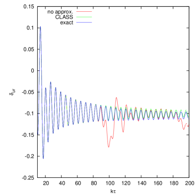
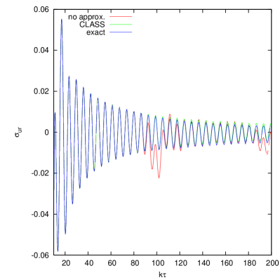
In Fig. 6, we compare the evolution of and for a given mode, obtained either by solving the full Boltzmann equation up to a very high , or with with/without the default UFA. In absence of approximation, one can see some spurious evolution appearing periodically (here, around and ): this corresponds to the propagation of an unphysical wave between the multipole boundaries and . Using the default UFA scheme ufa_class, we reproduce accurately the phase, the amplitude and, to a lesser extent, the zero-point of the oscillations. For the clarity of the figure, we do not show the results from alternative approximation schemes. We checked that the ufa_mb scheme also reproduces the correct phase and amplitude, but introduces a larger error in the zero-point of oscillations. Finally, the ufa_hu scheme reproduces the phase, but not the correct amplitude of the oscillations.
3.6 Comparison at the level of CMB/matter power spectrum
| UFA scheme (fixed and ) | ufa_none | ufa_class |
|---|---|---|
| rk | 29.7s | 27.0s |
| ndf15 | 16.7s | 15.2s |
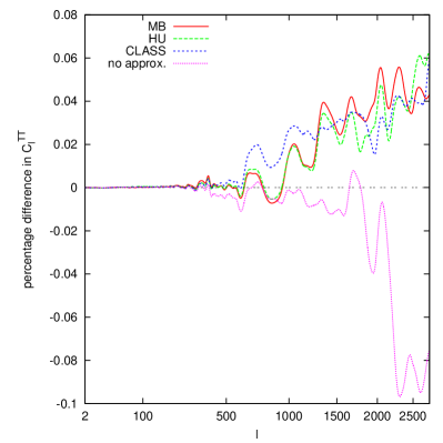
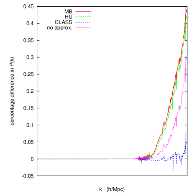
In Fig. 7, we show the impact of the UFA on the CMB and matter power spectrum. We take the precision parameters of the file cl_permille.pre, and play with the values of and , called l_max_ur and ur_fluid_trigger_tau_over_tau_k in the code. We first compute some reference spectra with (to remove any truncation effect), and such a large value of that the UFA is never used. All other results from this section are compared to these spectra. We then fix both and to 18 and vary only the ur_fluid_approximation parameter. We show the error induced by each UFA scheme for the temperature and matter power spectrum in Fig. 7 (results for temperature and polarisation are very similar). The results from the ufa_none case are very unstable and depend a lot on the choice of and ) values. With the present choice, they correspond to a twice larger error in the CMB spectra than in any UFA scheme; for slightly different choices they would also induce a larger error in the matter power spectrum. The three UFA schemes, which do not have such instabilities, are nearly as good as each other for CMB spectra, while for the matter power spectrum the ufa_class scheme is one order of magnitude better. Table 3 shows that the UFA approximation allows for a 10% speed up, while being more accurate for a fixed .
4 Radiation Streaming Approximation (RSA)
After their respective decoupling time, the photons gradually free-stream like neutrinos (except around the time of reionisation at which their coupling to baryons is enhanced). In principle, it would be possible to look for a fluid approximation for photons, like we did for neutrinos in the previous section. However we can go further than that, since during this period the universe is dominated by matter and eventually /Dark Energy: in this case photons and massless neutrinos almost behave like test-particles in an external gravitational field, and we do not need to catch their evolution with high accuracy (which was not the case for the ur species during radiation domination).
Like for massless neutrinos, in all efficient Boltzmann codes, the Boltzmann equation for photons is truncated at some low multipole value using the truncation scheme proposed in Ma & Bertschinger (Eqs. (65) in [10]). If is not large enough, the spurious reflection of power induced by the truncation propagates to the final results, because radiation perturbations still play a small role during the free-streaming regime. More precisely:
-
•
the photon density fluctuation, velocity and shear perturbations appear in Einstein equations;
-
•
the photon density fluctuation and shear appear in the temperature/polarisation source functions;
-
•
the photon velocity appears in the evolution equations of baryons (since the baryon-photon coupling is not negligible during reionisation).
In order to avoid propagating such an error, one can either increase , or find a way to infer the photon density, velocity and shear from some analytic Radiation Streaming Approximation (RSA), in which case the integration of Boltzmann equations can be stopped soon after photon decoupling. Mathematically, this analytic approximation should coincide with the particular non-oscillatory solution of the inhomogeneous Boltzmann equations. Once the damped oscillations accounted for by spherical Bessel functions becomes negligible (i.e. when ), the analytic approximation will coincide with the true solution. Before that time, it will provide a correct approximation to the true quantities averaged over a few oscillations. In summary, the RSA has a double goal: to avoid unphysical oscillations created by the Boltzmann truncation, and to avoid wasting time in integrating the Boltzmann equations over many such oscillations.
The RSA does not need to be accurate at very late time (end of matter domination, /Dark Energy domination), since by then radiation fluctuations are always completely negligible with respect to matter fluctuations. However, it should be reasonably accurate soon after photon decoupling, i.e. during matter domination, when the energy density in radiation, , is smaller than one but not yet much smaller. The advantage of a better approximation is two-fold. First, it can be switched on earlier. Second, before switching on the approximation, we can use a smaller value of , since high multipoles will not have time to grow.
The same treatment can be applied to ultra-relativistic species, which are identical to photons in this regime, except for the fact that they remain collisionless during reionisation. When the RSA is turned on for photons, it is better to follow ultra-relativistic species in the same way as photons, rather than with the fluid formalism described in Sec. 3. The RSA then removes three more differential equations, and cures the fact that the UFA turns out to be inaccurate at late time. Hence, the default version of CLASS treats ultra-relativistic species first with exact equations, then with the UFA (inside the Hubble radius and until photon decoupling), and finally with the RSA (inside the Hubble radius and after photon decoupling).
An expression for the RSA was discussed in the Newtonian gauge by Doran [11]. Soon after, a somewhat simpler RSA (neglecting reionisation) was also introduced in the CAMB code, which uses the synchronous gauge. Here, we will derive an approximation comparable to that of Doran [11], but valid in the synchronous gauge.
4.1 Relativistic relics (massless neutrinos)
We start with the simplest case, that of ultra-relativistic species ur. We combine the first two equations of (30) into
| (34) |
Inside the Hubble scale (i.e. when ) we can assume in first approximation that and neglect the shear in the RSA. Also, since we are looking for a smooth (non-oscillatory) particular solution of this inhomogeneous equation, we can assume that . We conclude that the RSA for is simply
| (35) |
Note that in the synchronous gauge, coincides with , where is the cold dark matter density contrast. Deep inside the matter-dominated regime, , so is linear in , and is a constant. The RSA for is therefore nearly static. Concerning , its value in the RSA is given by the exact energy-conservation equation , namely
| (36) |
In practice, we must extract and from the Einstein equations in the synchronous gauge, that read
| (37a) | |||||
| (37b) | |||||
| (37c) | |||||
Here we do not need the fourth equation sourced by the shear. The difficulty comes from the fact that in order to infer we should compute , and for doing that we need to combine the first and third equation, i.e. we need to know , which depends itself on . Fortunately, we can notice that if we omit in the computation of , we make a tiny error, since during matter domination . Hence, it is good enough to evaluate the first Einstein equation with set to zero. The same is not true for the second equation, since the synchronous gauge is comoving with cdm, so one has by construction. As a result, neglecting in the computation of and leads to a significant inaccuracy in the solution for . Hence, we introduce the following scheme:
-
1.
we compute assuming , and obtain from the first Einstein equation.
-
2.
using the fact that during matter domination , we notice that
(38) and hence to very good approximation
(39) We then infer the following RSA for from Eq. (35) :
(40) This formula is practical since is one of the variables that we integrate over time, and has been inferred in the previous step.
-
3.
We impose the free-streaming solution for (Eq. (36)) and set .
-
4.
We use the remaining Einstein, continuity and Euler equations to evolve the system.
4.2 Photons
For photons, the solution is a bit more complicated since the baryon-photon coupling cannot be neglected during reionisation. We then need to find the particular non-oscillatory solution of (cf. (4))
| (41) |
Once again we will neglect the shear and search for a particular solution slowly varying with time (). In order to deal with the coupling term, we expand the solution in powers of . The zeroth-order solution is exactly similar to that of massless neutrinos, Eqs. (40), (36). The first-order solution should satisfy
| (42) |
in which can be replaced using Eq. (39). This approximation turns out to work out very well, unlike the zeroth-order solution. The velocity is then given by the exact energy-conservation equation
| (43) |
We take the derivative of the previous result for , assuming that is time-independent, and using once more Eq. (39). We obtain:
| (44) |
in which can be replaced using Eq. (39). However the exact expression of depends again on . Like before, we use a perturbative scheme in and replace above by its expression at first-order in .
4.3 Summary of RSA equations
In summary, the RSA consists in neglecting and in the evolution of in the first Einstein equation, which allows us to obtain , and then in imposing
| (45a) | |||||
| (45b) | |||||
| (45c) | |||||
| (45d) | |||||
| (45e) | |||||
| (45f) | |||||
This scheme is set to be the default one in CLASS, as long as the precision variable radiation_streaming_approximation remains set to rsa_MD_with_reio. For comparison, some cruder schemes can be used: if the same variable is set to rsa_MD, the code will use the above expressions at zero order in (i.e, with and ). If it is set to rsa_none, the radiation perturbations are just set to zero.
4.4 Comparison at the level of perturbations
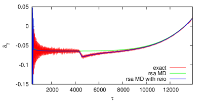
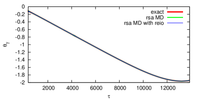
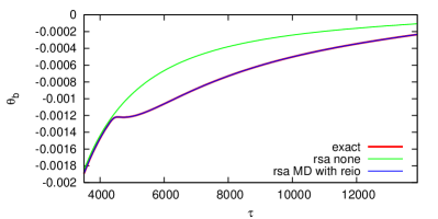
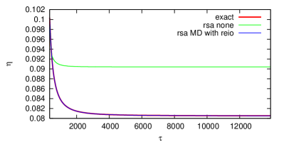
In Fig. 8, we show the evolution of , , and between recombination and present time, for a particular wavenumber Mpc-1. We compare two RSA schemes with the exact evolution obtained by integrating all multipoles at all times. We always keep the UFA approximation of Sec. 3 turned off. We see that immediately after switching on the RSA, our approximation for (and also for , which is not shown) matches accurately the exact evolution averaged over a few oscillations. This would not be the case with several simpler RSA schemes which assume full matter domination and an exact linear growth of . In the models used for the figures, reionisation takes place at and Mpc. It induces a clear feature in and (having impact on ) which is well captured by the terms proportional to in the full rsa_MD_with_reio scheme.
4.5 Comparison at the level of temperature/polarisation spectra
The precision parameters governing the evolution of perturbations in the late universe are:
-
•
two parameters defining the time at which the RSA is switched on. For each wavenumber, we stop evolving photon and ur perturbations when the two conditions
and
are satisfied (i.e., photons are sufficiently decoupled, and the wavelength is sufficiently deep inside the sub-Hubble regime). In principle, it would be possible to switch on the RSA at different times for photons and ur species, but for simplicity we did not consider this option.
-
•
l_max_g, l_max_pol_g and l_max_ur define the number of photon temperature, photon polarisation and ur multipoles which are integrated until the RSA is switched on.
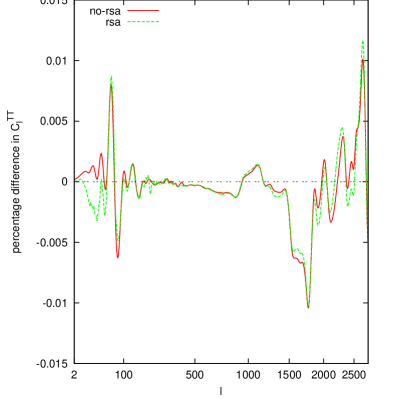
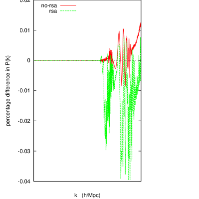
In order to compute some reference spectra to be used throughout this section, we fix the precision parameters according to the file cl_permille.pre, increase l_max_g, l_max_pol_g and l_max_ur to 3000, and choose such large values of the trigger parameters that the UFA and RSA are never employed. We wish to compare these reference spectra with those from runs with/without the RSA, in which l_max_g, l_max_pol_g and l_max_ur are kept fixed to reasonable values. We choose l_max_g and l_max_pol_g to be equal to 18. Since we do not want to use the UFA approximation in this comparison (in order to focus only on the impact of the RSA), we fix l_max_ur to a larger value, namely 50. This setting, called no-rsa in Table 4, leads to a 0.01% error both in the temperature multipoles and in the matter power spectrum for Mpc-1, as shown in Fig. 9. Finally, in the run called rsa, we switch on the default RSA scheme, with the trigger values specified in Table 4. With such settings, the error in the temperature (and also polarisation) multipoles remains as small as without the RSA, while the error in the matter power spectrum grows moderately to 0.04% (see Fig. 9). However, the running time is reduced considerably, as shown in Table 5: with the Runge-Kutta integrator, the RSA leads to a 66% speed up. Note that the ndf15 remains much better than the Runge-Kutta integrator when the RSA is employed (by a factor 2) while it experiences difficulties in following oscillatory solutions in absence of a RSA. However, the combination of our RSA scheme and ndf15 integrator leads to very nice performances (speed-up by a factor 4 with respect to Runge-Kutta without any RSA).
| precision setting: | reference | no-rsa | rsa |
|---|---|---|---|
| l_max_g | 3000 | 18 | 18 |
| l_max_pol_g | 3000 | 18 | 18 |
| l_max_ur | 3000 | 50 | 50 |
| radiation_streaming_trigger_tau_over_tau_k | 100 | ||
| radiation_streaming_trigger_tau_c_over_tau | 2 | ||
| ur_fluid_trigger_tau_over_tau_k |
| Runs with/without a RSA: | no-rsa | rsa |
|---|---|---|
| rk | 55.8s | 33.6s |
| ndf15 | 84.4s | 14.5s |
In CAMB, the RSA is somewhat cruder, since it neglects reionisation and uses an explicit cosmology-dependent relation giving an in terms of , , , and , valid only deep in the matter-dominated regime. We present in a companion paper the comparison between the matter power spectrum computed by CAMB and CLASS. In order to get an accurate with CAMB, one is forced to deactivate the RSA approximation (called late_rad_truncation), precisely for the above reasons. Our scheme does not lead to a significant error on the , and is more model-independent: it involves only metric perturbations and does not need to be modified in the presence of other components playing a role during matter domination (e.g. with warm dark matter or early dark energy).
5 Conclusions
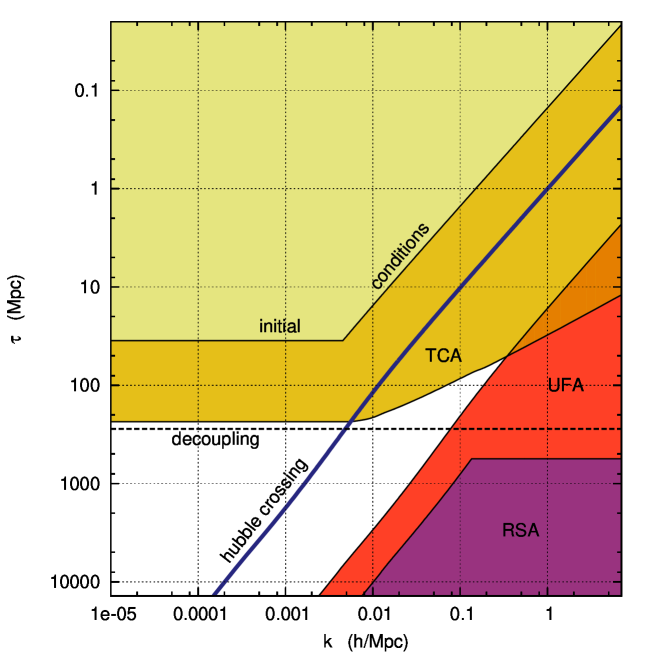
In Fig. 10, we summarise the different approximations used by the code in the plane when computing the ’s up to 3000 and the up to Mpc-1. The figure corresponds to the precision settings of the file cl_3permille.pre. Exact equations are used only in the band corresponding to Hubble crossing for each mode, as well as in the super-Hubble region with non-tightly-coupled photons, in which all quantities evolve very slowly and integration is very fast.
With these approximations, for CDM, the perturbation module only spends a significant time in the region corresponding to Hubble crossing for each mode, and to the sub-Hubble evolution before photon decoupling. At early times, stiff equations are avoided thanks to the Tight-Coupling Approximation. Well-inside the Hubble radius and until photon decoupling, the different modes oscillate and integration is time-consuming: however, the number of equations is kept small (of the order of 30 in total) thanks to the UFA. After photon decoupling, the code only needs to integrate over equations with very smooth solutions, and the time spent by the code in the RSA region is negligible.
Other approximation schemes can be introduced in more general cosmological models. The case of massive neutrinos and non-cold dark matter relics is discussed in a companion paper. More exotic cases may require further approximations which can be introduced and discussed case-by-case (CLASS is coded in such way that introducing a new approximation is as structured, codified and simple as introducing new species [6]). However, the fact that CLASS uses an original stiff integrator means that for several purposes (as for the generalisation of TCA), new approximation schemes are not even strictly necessary.
Acknowledgments
This work was supported in part by the Swiss Science Foundation (D.B.). Running with high-precision settings is only practical on machines with many cores and large memory: we wish to thank M. Shaposhnikov for providing us with a brand new 48-core PC at EPFL, and the Institut d’Astrophysique de Paris for giving us access to the horizon9 machine. Finally, we would like to thank A. Lewis for many useful comments.
References
- [1] E. Bertschinger, arXiv:astro-ph/9506070.
- [2] U. Seljak, M. Zaldarriaga, Astrophys. J. 469 (1996) 437-444. [astro-ph/9603033].
- [3] A. Lewis, A. Challinor, A. Lasenby, Astrophys. J. 538 (2000) 473-476. [astro-ph/9911177].
- [4] M. Doran, JCAP 0510 (2005) 011. [astro-ph/0302138].
- [5] J. Hamann, A. Balbi, J. Lesgourgues, C. Quercellini, JCAP 0904 (2009) 011. [arXiv:0903.0382 [astro-ph.CO]].
- [6] J. Lesgourgues, “The Cosmic Linear Anisotropy Solving System (CLASS) I: Overview,” [arXiv:1104.2932 [astro-ph.IM]].
- [7] J. Lesgourgues, T. Tram, “The Cosmic Linear Anisotropy Solving System (CLASS) IV: efficient implementation of non-cold relics,” [arXiv:1104.2935 [astro-ph.CO]].
- [8] J. Lesgourgues, “The Cosmic Linear Anisotropy Solving System (CLASS) III: Comparison with CAMB for LambdaCDM,” [arXiv:1104.2934 [astro-ph.CO]].
- [9] P. J. E. Peebles and J. T. Yu, Astrophys. J. 162 (1970) 815.
- [10] C. P. Ma and E. Bertschinger, Astrophys. J. 455 (1995) 7 [arXiv:astro-ph/9506072].
- [11] M. Doran, JCAP 0506 (2005) 011. [astro-ph/0503277].
- [12] F. -Y. Cyr-Racine, K. Sigurdson, [arXiv:1012.0569 [astro-ph.CO]].
- [13] W. Hu, Astrophys. J. 506 (1998) 485-494. [astro-ph/9801234].
- [14] C. Pitrou, Phys. Lett. B 698 (2011) 1 [arXiv:1012.0546 [astro-ph.CO]].
- [15] S. Naoz, R. Barkana, Mon. Not. Roy. Astron. Soc. 362 (2005) 1047-1053. [astro-ph/0503196].
- [16] A. Lewis, Phys. Rev. D76 (2007) 063001. [arXiv:0707.2727 [astro-ph]].
- [17] Shampine, Lawrence F. and Reichelt, Mark W. SIAM J. Sci. Comput. vol. 18, 1 (1997)
- [18] Davis, Timothy A. SIAM J. Sci. Comput. vol. 18, 1 (1997) Direct Methods for Sparse Linear Systems
- [19] M. Shoji, E. Komatsu, Phys. Rev. D81 (2010) 123516. [arXiv:1003.0942 [astro-ph.CO]].
- [20] M. Bucher, K. Moodley, N. Turok, Phys. Rev. D62 (2000) 083508. [astro-ph/9904231].
Appendix A Stiff integrator
The standard numerical method for solving Ordinary Differential Equations (ODEs) is to use an adaptive step size Runge-Kutta solver. While this method is fast and accurate in simple cases, it may fail completely (or take a very large number of steps) when the problem is stiff. Stiffness occurs when at least two times scales of evolution in the problem differ substantially. A well known example is the Boltzmann equation in cosmology. If a distribution is kept in equilibrium by the (rapid) interaction with a background species, and we are interested in the evolution of the distribution on cosmological time-scales, a Runge-Kutta solver will oscillate around the equilibrium solution by means of very small time steps related to the time-scale of the interaction.
This problem exists, for instance, in the early universe where baryons and photons are strongly coupled. One solution is to substitute the equilibrium solution into the equations and thereby reducing the system of equations and removing the stiffness: this is the basic principle of the Tight Coupling Approximation (TCA) discussed in Sec. 2. This approximation removes the stiffness of the Boltzmann equation in the vanilla scenario.
However, stiffness may easily be reintroduced by trying to incorporate new physics into the code. The proper TCA approximation should then be derived and implemented in the code, which would require a great deal of familiarity with the code from the user. In CLASS, however, the user can just take advantage of the implemented stiff solver.
The ndf15 algorithm is a variable order (1-5) adaptive step size solver based on the Numerical Differentiation Formulas of order 1 to 5. The step size is adaptive but quasi-constant, meaning that the formulas used are based on a fixed step size. Each time the step size changes, the code will update the backward differences by interpolation to reflect this new step size. The algorithm is described in [17].
Whereas Runge-Kutta methods are explicit, meaning that the next step can be computed directly from the previous step by elementary operations, ndf15 is a fully implicit method. This means that at each time step, we must solve a system of algebraic, possibly non-linear equations, which is accomplished by Newton iteration. This requires a numerical computation of the Jacobian and the solution of systems of linear equations. As it is evident, all this can make each step very expensive, so a number of strategies must be implemented:
-
•
Reusing Jacobians:
The Jacobian usually changes more slowly than the solution itself, so an attempt is made to reuse the Jacobian - it will only be recomputed if Newton iteration is too slow.
-
•
LU decomposition:
The same linear system must be solved repeatedly with different right hand sides, so we should of course store an LU decomposition. Because the system of equations can be large, , we need sparse matrix methods for this.
-
•
Backward Interpolation:
Since the method stores a matrix of backward differences, it is fast to infer the value and the derivatives of the solution at points before the current point by interpolation. We only need the values of some of the components to calculate the source functions, so we do not need to interpolate the rest of them.
When the number of equations is larger than about , it is advantageous to use sparse matrix methods, and if the system is somewhat larger, the difference in execution time can differ by orders of magnitude. Usually sparse matrix methods are developed in order to save both time and memory, but for our purposes only execution time matters. We created a small sparse matrix package for our purpose based on [18]. Some important features of this package are:
-
•
Column Pre-ordering:
The matrices which appear are of the general form where is the identity matrix, is the Jacobian and is some constant. Since the Jacobian is close to being structurally symmetric (if couples to , it will often be the case that couples to ), it is advantageous to use the Approximate Minimum Degree column ordering of the matrix . Using this pre-ordering reduces the number of non-zero elements in the corresponding L and U factors by a factor of a few, which leads to a sizable reduction in the time needed to solve the linear systems.
-
•
LU re-factorisation:
If we have already calculated a LU factorization for some Jacobian, which is structurally identical to the current Jacobian, we can use information saved during the factorisation of the former to factorise the new matrix in a fraction of the time. Specifically, we store the pivot ordering and the reach of all the sparse right hand sides used in forming the LU-decomposition.
-
•
Fast Jacobian Calculation:
If the same pattern of the Jacobian is found repeatedly, we can use this pattern to speed up the calculation. Taking advantage of the sparsity of the Jacobian, we can group the columns together and form the Jacobian using only a fraction of the usual function evaluations, being the number of equations.
The CLASS user can choose to use the Runge Kutta or ndf15 integrator by switching the precision parameter evolver to either rk (=0) or ndf15 (=1, default setting). To illustrate the power of ndf15 in stiff situations, ndf15 was less than 10% slower when the TCA was turned off as early as in the reference run used in Fig. 2. As a comparison, the standard Runge-Kutta integrator was more than 10000 times slower than ndf15 for the same model. This particular run represents an extreme case, but throughout this work we have presented various examples in which the ndf15 performances are very good.
Appendix B Derivation of fluid equations for ultra-relativistic relics
The goal of this Appendix is to establish the validity of the approximate shear derivative equation (31), which allows to treat collisionless species as an imperfect fluid governed by may less equations. In the future, our results could be used for computing higher order terms in (31), or more generally for understanding various properties of the linear perturbations of ultra-relativistic species. A discussion similar in spirit was presented in [19] for massive neutrinos, although the goal of that paper was to introduce a sharp truncation at , while we are searching for a truncation scheme that would take into account the transfer of power to higher ’s.
B.1 Formal solution
Sticking to the notations of Ma & Bertschinger, the perturbations of ultra-relativstic species is described by a function obeying to the collisionless Boltzmann equation
| (46) |
where stands for the gravitational source terms. The most general formal solution can be written as
| (47) |
The initial function depends on the considered gauge and type of initial conditions. For instance, in the synchronous gauge, for the growing ADiabatic (AD), Baryon Isocurvature (BI) and Cold Dark Isocurvature (CDI) modes; has a non-zero monopole term for Neutrino Isocurvature Density (NID) initial conditions; and a non-zero dipole term for Neutrino isocurvature Velocity (NIV). These statements can be checked from ref. [20]. Hence, in all cases, we can write
| (48) |
More fundamentally, the fact that only has monopole and dipole contributions can be justified by the fact that neutrinos were initially in thermal equilibrium, forming a fluid with no anisotropic pressure or higher momenta. By causality, this remains true at any time after decoupling on super-Hubble scales. So, we are sure that the above form of is completely universal. In the synchronous gauge, the source reads
| (49) |
Thanks to a few integration by part, it is possible to absorb the dependence, in order to be able to write this solution in Legendre space. The result is
| (53) | |||||
The last bracket contains the initial value of ( and . The former vanishes for all types of initial conditions excepted NIV; the latter is non-zero for AD, NID and NIV. All initial condition terms in the first and last lines can be grouped and represented by two coefficients and :
| (54) | |||||
| (55) |
with e.g. for adiabatic initial conditions (as can be checked from [20]), being the fractional contribution of ultra-relativistic species to the background density. It is now easy to expand the full solution in Legendre coefficients, using the definition and the fact that plane waves can be expanded in terms of spherical Bessel functions:
| (58) | |||||
The terms in the first line show how initial conditions propagate to later times, by just free-streaming. The other terms show how perturbations adjust themselves to the power injected in the system at any time by metric perturbations.
B.2 Sub-Hubble approximation
Well inside the Hubble radius, the above formal solution can be approximated by a simpler expression. The results of this subsection are never used in our UFA scheme or in CLASS, but we present them for completeness, and also because the approximation performed in the next subsection will follow the same logic.
The second line of the solution contains a convolution between a function which varies smoothly over a Hubble time (at least for ), and a Bessel function with which oscillates over . Bessel functions peak near (in fact this statement is accurate only for very large ; for instance, peaks near and near ). The integral on corresponds to . The goal of this subsection is to find an approximation for this convolution for small values.
As long as , it is difficult to find a low- approximation for the convolution; the result is a function oscillating over a characteristic time . In this regime, the integral brings an extra oscillatory contribution to the term ; this explains while around Hubble crossing, the numerical solution for exhibits irregular oscillatory patterns, with very different peak amplitude between two consecutive periods.
However, when , the integral runs over a large range . For low , this means that the convolution picks up significant contributions only near . Near this value, the slowly-varying argument can be approximated as a constant, to be evaluated around , i.e. in very good approximation near , since . So, we can write:
| (59) |
Finally, still in this limit , the last integral can be approximated by
| (60) |
A more accurate approximation scheme would lead to extra contributions involving time derivatives of the quantity between brackets in (59): for instance, the next order term would be of the type
| (61) |
with being a coefficient of order one. However, since inside the Hubble scale metric perturbations vary over a Hubble time , we can keep only the leading source terms with the highest power of :
| (62) | |||||
| (63) | |||||
| (64) |
In the code, we do not use directly these asymptotic approximations, and try instead to close the system of differential equations with a trunction at order two, like for a viscous fluid.
B.3 Exact truncation formula
First, in order to manipulate more compact equations, we define:
| (65) |
Since and contains a term , we suspect that it obeys approximately to a similar relation. We use equation (58) for computing exactly the difference , which would vanish if only the term was contributing. We use the identities
| (66) |
and . We find
| (67) | |||||
where we defined
| (68) |
This expression simplifies to
| (69) |
This trunction scheme is not pratical in general. However, the goal of the UFA is to find a way to close the system at low not at all times, but only deep inside the Hubble radius.
B.4 Sub-Hubble truncation formula
In the limit , equation (67) can be simplified for two reasons. First, the Bessel function varies over a time scale , so
| (70) |
Hence, in this limit, the last term in the identity (66) can be omitted, which implies that the first term (proportional to ) in eq. (67) is always negligible, even in the presence of isocurvature modes. Second, we can devise an approximation for the convolution, by noticing once more that it involves metric perturbations wich vary smoothly over a Hubble time (at least for ), and the quantity with which oscillates over a period of order .
When , the integral runs over a large range . For low , this means that the convolution picks up significant contributions only near , while in this range . Near , the slowly-varying metric perturbations can be treated as a constant term. So, we can write:
| (71) | |||||
with
| (72) |
Let us estimate the error made in these approximations. Since we are inside the Hubble radius with smoothly varying metric perturbations, and since the integral in eq. (71) is of order , the leading term in eq. (71) is of order . The other terms of order and can be neglected. If instead of considering as a constant we perform a Taylor expansion of this function around , we find that the next order contribution to eq. (71) is of order . Finally, an explicit calculation shows that the approximation performed in (72) amounts in neglecting terms of order with respect to terms of order . In summary, we obtain the following approximate truncation equation:
| (73) | |||||
For , the integral is equal to -1/3, since and . So,
| (74) |
Replacing the ’s by the appropriate momenta, we find:
| (75) |
The last term comes from our approximation for the convolution. Without a full treatement like the one presented here, one would miss this term and obtain the truncation formula called ufa_mb in the code, based on simply assuming . However, with this extra contribution, the two terms in cancel each other, and at leading order we end up with
| (76) |
which is precisely what we call the ufa_class truncation scheme in CLASS.