LAPTH-1236/08
How to constrain inflationary parameter space with minimal priors
Abstract
We update constraints on the Hubble function during inflation, using the most recent cosmic microwave background (CMB) and large scale structure (LSS) data. Our main focus is on a comparison between various commonly used methods of calculating the primordial power spectrum via analytical approximations and the results obtained by integrating the exact equations numerically. In each case, we impose naïve, minimally restrictive priors on the duration of inflation. We find that the choice of priors has an impact on the results: the bounds on inflationary parameters can vary by up to a factor two. Nevertheless, it should be noted that within the region allowed by the minimal prior of the exact method, the accuracy of the approximations is sufficient for current data. We caution however that a careless minimal implementation of the approximative methods allows models for which the assumptions behind the analytical approximations fail, and recommend using the exact numerical method for a self-consistent analysis of cosmological data.
1 Introduction
Cosmic inflation is the simplest and most robust paradigm capable of providing self-consistent initial conditions to the Hot Big Bang scenario [1, 2, 3, 4, 5, 6], as well as a mechanism for the quantum-gravitational generation of primordial scalar (density) perturbations and gravitational waves [7, 8, 9, 10, 11, 12, 13]. The Fourier power spectrum of the former is observed today in the cosmic microwave background (CMB) and the large scale structure (LSS). Vice versa, at present the CMB and the LSS provide the only quantifiable observables which can confirm or falsify inflationary predictions. That is why matching concrete inflationary models to observations has become one of the leading quests in cosmology.
In the standard inflationary picture, the amplitude of perturbations for a given comoving Fourier mode depends crucially on the dynamics of inflation around the time of Hubble exit for this mode. Each Hubble exit time is conveniently parameterised in terms of the number of -folds before inflation ends. The relation between and depends very much on the overall energy scale of inflation. The ensemble of modes observable in the CMB and in the quasi-linear part of the LSS power spectra corresponds to a range called “observable inflation”. The total duration of inflation is a priori unlimited, but the number of -folds between the time at which the presently observable Universe became as large as the Hubble radius and the end of inflation can only vary in the approximate range , that will be called “relevant inflation” throughout this paper.
The literature on inflation constraints is plethoric. For simplicity, a majority of papers are restricted to the case in which inflation is driven by a single scalar field (an inflaton) with a canonical kinetic term, some potential and minimal coupling to Einstein gravity (however, each of these assumptions can be relaxed and has already been studied separately). Traditional works are based on the definition of spectral parameters (amplitude, index, possibly running) for density perturbations and gravitational waves. In a first step, these parameters are fitted to the data; in a second step, one tries to infer the class of inflationary models compatible with derived bounds on spectral parameters.
In the last years, many works have gone beyond this approach, recognising that the introduction of spectral parameters puts already a strong theoretical prior on the models, and is by no means a necessary step. It is more realistic and equally efficient to fit directly to the data the (more fundamental) parameters governing the dynamics of inflation and/or the inflaton potential. Within the main stream (standard single field inflation), recently published analyses fall in two categories which are both interesting and complementary: either one assumes a particular model based on a definite form for the inflaton potential throughout relevant inflation, and derives constraints on the free parameters of this potential (top-down approach); or one employs a generic parameterisation of the potential or another function governing inflationary dynamics, e.g. , and tries to reconstruct this function from the data (bottom-up approach). The second approach aims at avoiding theoretical priors as much as possible, and concentrating on what the data exactly tells us, although no parameterisation can be completely general: sharp features are usually excluded ab initio (obviously, all possible features cannot be accounted for with a reasonable number of free parameters). Even within the bottom-up approach, a distinction can be established between conservative analyses reconstructing only the part of corresponding to observable inflation; and more aggressive analyses in which the potential (or the function ) is extrapolated till the end of inflation, and subject to a prior on the minimum duration of relevant inflation (e.g. ). This more aggressive method should imply varying many more parameters, since in this case the parameterisation should be accurate over 30 to 60 -folds instead of just . The fact of extrapolating is by itself an extra theoretical prior, since cosmological data tell us essentially nothing about the era between observable inflation and Nucleosynthesis: the end of inflation could be subject to multi-field dynamics, experience phase transitions, be split into several non-contiguous short inflationary stages, etc.
Here we address only the most conservative approach, i.e., the reconstruction of the inflationary dynamics during observable inflation, with a minimal number of assumptions. After the publication of WMAP results, this approach was followed in Refs. [14, 15, 16, 17, 18]. It was stressed in [14, 15, 16] and [18] that the quantity primarily constrained by the data is : hence, this function is the one which should be parameterised in some way and fitted to the data. The knowledge of uniquely defines the potential , and Ref. [18] presented the collection of potentials corresponding to the ensemble of functions allowed by current WMAP and SDSS LRG data. The results are still plagued by degeneracies: since the energy scale of inflation is unknown, the data favors a parametric family of inflaton potentials rather than a precise shape within the observable window. However, a lot of improvement is expected from the next generation of CMB experiments, especially the planck satellite. The reconstruction of observable inflation will improve spectacularly if primordial gravitational waves are observed by planck or another experiment, in the form of polarised -modes. This would fix the tensor-over-scalar ratio , and hence the energy scale of inflation. Even without -modes, the Planck data would provide -dependent constraints on the inflation potential of unprecedented precision. In this perspective, it is worth comparing the details and merits of each reconstruction method.
Choosing to concentrate on the reconstruction of during observable inflation does not fix the method entirely, in particular as far as the computation of the primordial spectra is concerned. The authors of [14, 15, 16] employed analytic approximations of two different forms, while those of [18]111Numerical spectrum computations were also employed in various complementary approaches to the problem of constraining inflation, based on definite potentials [19, 20, 21, 22] or on a frequentist analysis with extrapolation of the potential throughout relevant inflation [23]. wrote a module appended to CAMB [24] and CosmoMC [25], which derives the numerical spectra for each new set of inflationary parameters by numerically solving the exact equations. It is interesting to study whether the difference between these methods is relevant given the precision of current and future data. Beyond the issue of perturbations, different methods could also differ through different assumptions concerning the parameterisation of the background evolution, and the exact number of -folds during which this parameterisation is (explicitly or implicitly) assumed to hold and be compatible with accelerated expansion. The goal of this paper is to compare in details these different techniques, and to see how each difference impacts the constraints obtained from current data. Although current inflaton potential reconstructions are still dominated by degeneracies, a careful understanding will be necessary before applying these methods to the highly precise data expected in the next years.
In the next section we will briefly review the theory of inflationary perturbations and discuss the exact approach, as well as two commonly used approximative methods for the calculation of the primordial perturbation spectra. In section 3, we will present the results of an analysis of current data and demonstrate that the bounds using the approximative methods with a naïve prior differ significantly from the constraints inferred with the exact method. We will track down the cause of these differences and compare the accuracy of the approximations in section 4 before we conclude in section 5.
2 Background and perturbations in single field inflation
The observable spectra of density perturbations and gravitational waves are directly related to the evolution of the Hubble parameter as a function of in the neighbourhood of an arbitrary pivot value . The function can in principle be reconstructed from the data without any need to assume an explicit value of . Each defines a unique set through
| (2.1) | |||||
| (2.2) |
whenever 222Such a singularity is never reached as long as is used as the defining quantity and has an analytic expression over the range considered. As mentioned in Ref. [18], can be reached for a field value only if has a non-analytical expression like in the vicinity of . This cannot happen with the parametrisations used in this work (polynomial expressions for either or ). In addition, reaching would imply that the field changes direction with an opposite sign for , which is not compatible with the assumption of a single-valued function . (the prime denotes a derivative with respect to , and we have set ). In Ref. [18], the defining quantity was Taylor-expanded up to the cubic term:
| (2.3) |
which is equivalent to keeping the first three slow-roll parameters
| (2.4) | |||||
| (2.5) | |||||
| (2.6) |
in the Hubble flow hierarchy [26, 27], as in the slow-roll reconstruction approach of Refs. [28, 14, 15, 16]. Note that the universe expansion remains accelerated as long as . For practical purposes, any parameterisation of could be used when fitting the data with a Bayesian MCMC analysis. Besides the issue of priors on inflationary parameters, each parameterisation corresponds to a different ensemble of possible inflationary models. One can wonder how much the final results (i.e., the range of allowed potentials) depends on the parameterisation. In the following analysis we will compare the results obtained by Taylor-expanding either or at the same order, using in both cases the same flat priors on the first slow-roll parameters expressed at the pivot scale .
Once the ensemble of possible inflationary models has been specified, the analysis still depends on the way to calculate the perturbation spectra in single-field inflation, and on a theoretical prior on the duration of inflation. In this section we will give a very brief summary of three different approaches used in Refs. [14, 15, 16, 18]. Keep in mind that throughout this paper, we are working under the assumption of a minimal prior. In other words, we do not impose any lower bounds on the number of -folds of inflation, we only demand that the spectra of a model can be calculated with the respective methods. So, besides possible differences in the accuracy of the resulting spectra, the default implementation of the three methods will also differ in the range of parameter values that would be excluded straight away.
2.1 Exact spectra via mode equation
Given as a function of during inflation, the spectrum of curvature perturbations and gravitational waves can be calculated exactly by integrating the scalar/tensor mode equation (see, e.g,. [29]):
| (2.7) |
with and for scalars, for tensors. The evolution of the background is determined by
| (2.8) |
The are usually taken to be in the Bunch-Davies vacuum when they are well within the horizon, and their evolution needs to be tracked until converges to a constant value, in order to define the observable spectra:
| (2.9) |
In principle, observable inflation could be interrupted for a very short amount of time, resulting in characteristic features in the spectra. In the mainstream approach, this situation is not considered for simplicity. Actually, the numerical module used in Ref. [18] eliminates models violating at any point during the period of time the mode equation is integrated. More precisely, for any wavenumber in the range Mpc-1 needed by CAMB (the pivot scale being fixed at Mpc-1), the module integrates Eq. (2.7) from the time at which and until . If for a given function the product does not grow monotonically by a sufficient amount for fulfilling the above conditions, the model is rejected (we recall that it is equivalent to impose that grows or that is greater than one).
The condition is motivated by our desire to obtain a 0.1% accuracy in the power spectra. The error made on by stopping the integration of perturbations at a finite time can be estimated analytically, comparing the amplitude of the decaying mode to that of the non-decaying mode for or gravitational waves during inflation. The decaying over non-decaying mode ratio evolves in a first approximation like , i.e., like . Hence, a few lines of algebra show that the derivative is a good approximation for the relative error produced by stopping integration at a finite time. Other parameters governing the precision of the power spectra calculation (like the step of integration, the choice of the initial integration time for each mode, etc.) where chosen in such way that the above source of error is the dominant one.
The numerical evaluation of the spectrum involves solving equations (2.7) for each value of , but this does not increase the total running time of a Boltzmann code like CAMB by a noticeable amount. Nevertheless, there exist a number of approximations in the literature, which simplify the calculation considerably.
2.2 Approximation I
This method was employed in [14, 16], and relies on the validity of the analytical slow-roll approximations,
| (2.10) | |||||
| (2.11) |
with , where is the Euler-Mascheroni constant. These equations were first derived in [30] and are accurate only to first order in the slow-roll parameters, assuming additionally that and are constant. Here, one only needs to solve one differential equation to determine ,
| (2.12) |
assuming . Once is known, the slow-roll parameters and hence the spectrum can be evaluated for each value . In this approach, the evolution of Eq. (2.12) has to be followed throughout the observable range of wavelengths. If , equation (2.12) will diverge, so models with within this range will have to be excluded when using this method. If however, the inflationary condition were violated just before or after this range, the model would not be ruled out, and the resulting spectra would likely be inaccurate.
2.3 Approximation II
This method is based on the usual Taylor-expansion of the spectra in log-space around a pivot scale (see e.g., [31, 32]),
| (2.13) | |||||
| (2.14) |
with the spectral indexes , and the running of the scalar tilt given by their second-order slow-roll expressions
| (2.15) | |||||
| (2.16) | |||||
| (2.17) |
where . The slow-roll parameters only need to be evaluated at a field value , corresponding to the time when leaves the horizon. and are calculated from equations (2.10) and (2.11), and the spectra follow directly. One does not need to solve any differential equations here, so the numerical implementation of this method is by far the simplest of the three. However, due to the additional assumption on the shape of the spectrum, it becomes increasingly inaccurate the further one goes away from the pivot scale.
Apart from that, in the spirit of choosing a minimal prior one would typically rule out only those models that break the condition at the pivot scale, thus allowing regions in parameter space in which inflation would break down even within the observable range and making the prediction of the spectra for these models extremely unreliable.
3 Constraints from current data
In this section we present the constraints on inflationary parameter space from a selection of current observations, comprising CMB data from the WMAP [33, 34], Boomerang [35, 36, 37] and ACBAR [38] experiments, complemented by the galaxy power spectrum constructed from the luminous red galaxy sample of the Sloan Digital Sky Survey [39]. We analytically marginalise over the luminous to dark matter bias and the nonlinear correction parameter .
We consider a CDM-model with eight free parameters, on which we impose flat priors. Four of these parameters determine the initial perturbation spectra: the scalar normalisation , and the first three slow-roll parameters: , and , evaluated at the pivot scale Mpc-1. We emphasise once more that the numerical computation of perturbations does not refer to any slow-roll expansion, and remains self-consistent even when the field is not rolling very slowly. The fact of varying parameters which coincide with the usual slow-roll parameters is just a choice of prior in parameter space, which is particularly convenient for two reasons: first, the posterior is well-behaved with respect to these parameters and the convergence of the chains is achieved in a reasonable amount of time; second, it facilitates comparison with other works. The remaining four parameters are the baryon density , the cold dark matter density , the ratio of sound horizon to angular diameter distance at decoupling , and the optical depth to reionisation . We use a modified version of the Markov-Chain-Monte-Carlo code CosmoMC [24, 25] to infer constraints on the free parameters of the model. The inflation module was made publicly available by the authors of Ref. [18] at http://wwwlapp.in2p3.fr/~valkenbu/inflationH/.
3.1 Expansion in vs. expansion in
We first check the impact of changing the parameterisation of (i.e., the precise ensemble of inflationary models considered) from a Taylor-expansion of order 3 in to the same expansion in . In both cases, we used the same priors on inflationary parameters: hence the difference only resides in the fact that slightly different background evolutions can be achieved in both cases. The differences are summarised in table 1 and turn out to be very minor. This preliminary analysis shows that the parametric form assumed for within the observable window has a minor impact. Significant differences could only be expected if the choice of parameterisation of would allow much more freedom in one case than in the other.
| 0 0.028 | 0 0.023 | |
| -0.035 0.046 | -0.035 0.039 | |
| -0.0026 0.028 | -0.0053 0.027 |
3.2 Approximations vs. exact spectra
Our results are presented in figures 1 and 2. We do not find any significant differences in the posterior probabilities of , , and . The four parameters that determine the primordial spectra, however, are more sensitive to the method used. Note that the exact method produces tighter bounds on the slow-roll parameters, particularly on .
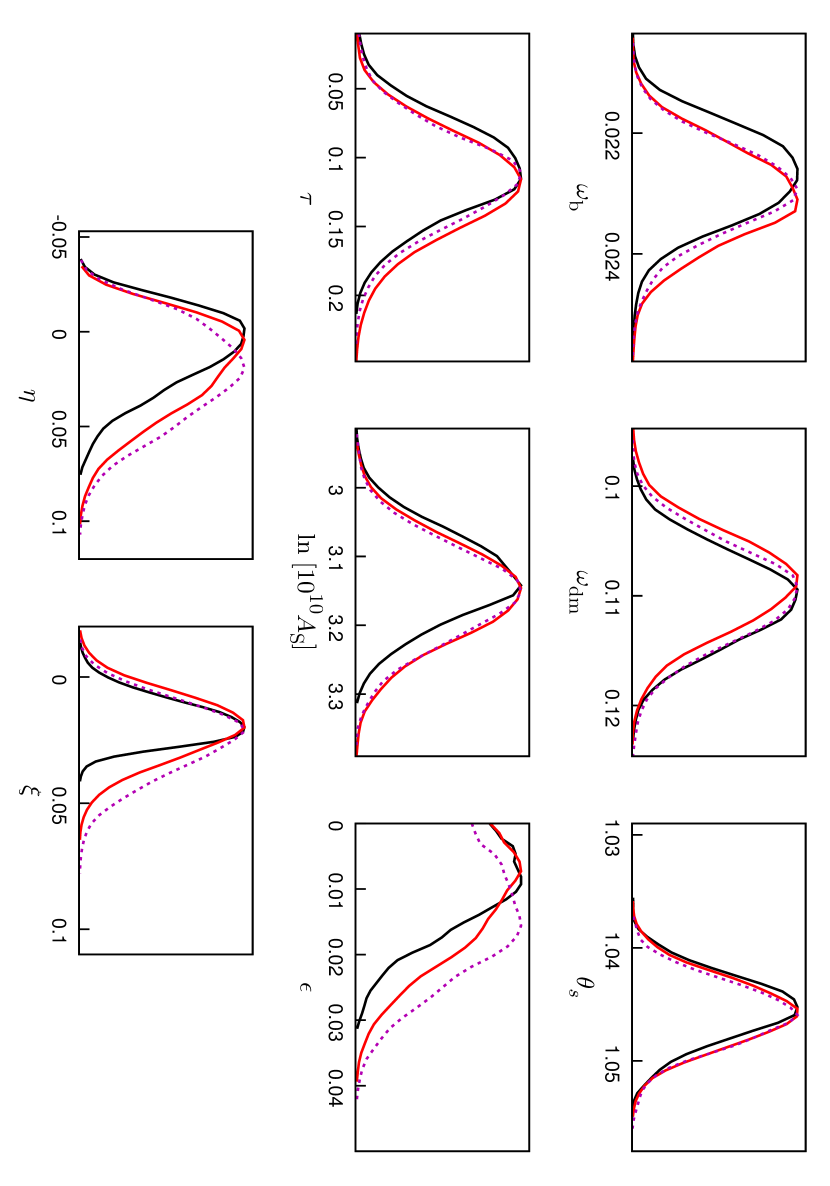
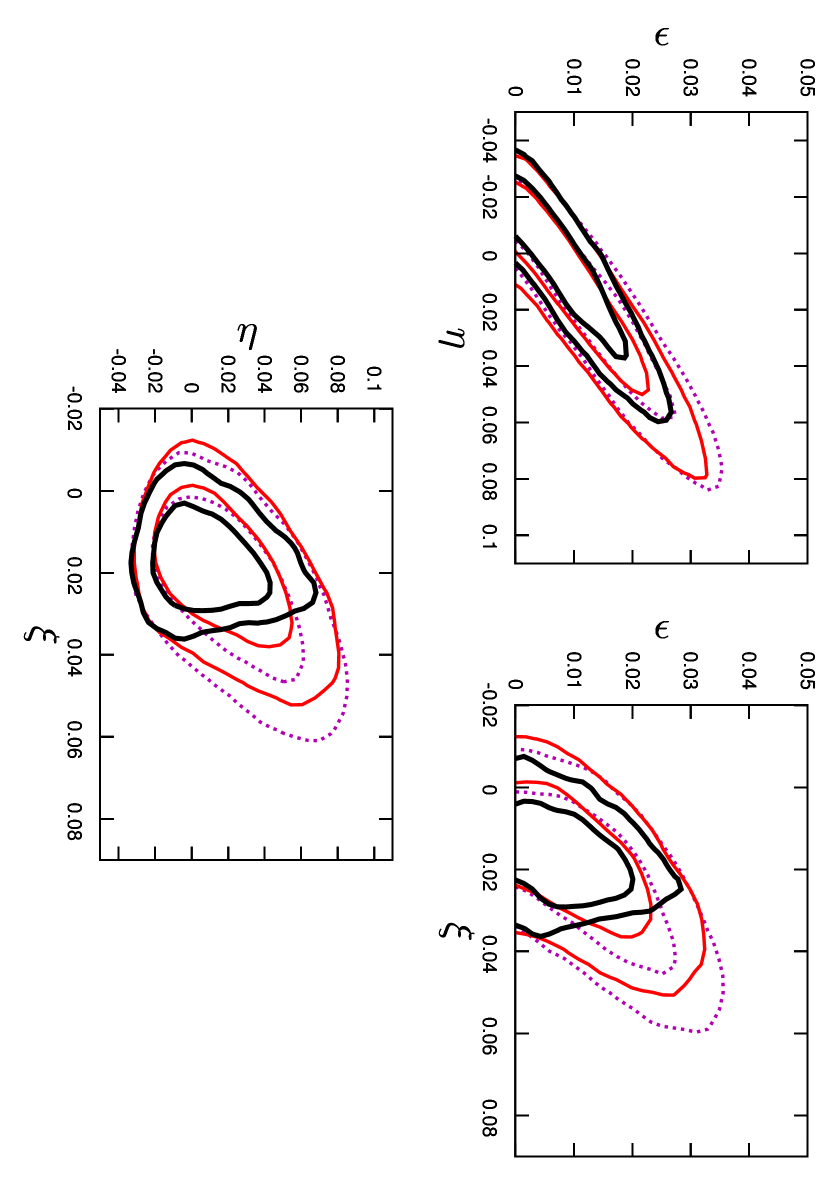
This also has important consequences on the inferred values of derived phenomenological parameters, such as the spectral index and its running. As can be seen from table 2, the exact method yields significantly stronger constraints on these two parameters.
| exact | approximation I | approximation II | |
|---|---|---|---|
4 Why the difference?
There are potentially two reasons for these observed discrepancies. The first one is that the accuracy of the approximations could be insufficient within their respective “allowed” parameter space and lead to a serious bias in the parameter estimates. Note that the discrepancy occurs mostly in regions of parameter space where is large. The larger , the more one would expect the accuracy of the approximations to degrade. However, given that the approximations are expected to be accurate to order , i.e., not worse than , an effect as large as the one we observe seems rather unlikely.
The second reason is slightly more subtle: as we discussed in section 2, the three methods differ in their implicit prior on the space of models. While approximation II requires only at the pivot scale, approximation I needs us to demand that this condition be fulfilled in the entire observable window of -folds, corresponding to Hubble exit for modes in the range. In the exact numerical approach, we require for the whole integration time, which starts when instead of one, and ends when freezes out, i.e., a few -foldings after , corresponding to an even more restrictive prior.
It was pointed out in Refs. [15, 40] that for models with large positive values of () and no higher derivatives, inflation tends to end within a few -foldings of the pivot scale leaving the horizon333If higher derivatives are present this conclusion can be weakened, see, e.g., [41, 42].. This is consistent with our results, since the more restrictive priors lead to tighter bounds on .
4.1 The prior issue
To verify that the differences actually stem from the choice of priors and not from a lack of accuracy, we post-processed our Markov chains of the approximate methods, discarding all models for which inflation is interrupted in the range of wavelengths required for the exact calculation.
In a first step, we remove only those models for which the inflationary condition is violated before the pivot scale leaves the horizon, when is in the range . These are models for which the assumption of the Bunch-Davies vacuum initial condition is violated at least for the largest observable wavelengths. Only a mere 0.02% of the models in the chains using approximation I, and 0.01% for approximation II, fall victim to the cut444Here, and in the following, we quote a weighted fraction of models, i.e., , where are the statistical weights of the points in the Markov chains, and are the weights of the models killed by the prior.. This is probably connected to the dislike of the data for models with large negative , which is required if we want inflation to start only just before the observable range.
Imposing the same additional prior as in the exact method (that inflation holds till the time of freeze out for each mode), of the approximation I points and of the approximation II points are removed. After weeding out the bad models, the bounds of the approximations perfectly agree with the ones derived using the exact method, their marginalised posteriors are virtually indistinguishable. This confirms our suspicion that the different priors are responsible for the discrepancy between the methods.
4.2 Comparison of accuracy
Having seen that the prior plays a very important role, it is nonetheless interesting to take a closer look at how the approximations compare to the exact method in terms of accuracy.
In order to compare the accuracy of the three methods described previously, we took the 95% best-fitting spectra obtained using approximations I and II and for each model in the chains we again computed the curvature spectrum in either of the approximations and numerically in order to compare. We searched for the maximum discrepancy between the approximated spectrum (with method I or II) and the numerical one, in each of the two ranges and , with , , , in units of 1/Mpc, corresponding to the range of wavelengths the data are most sensitive to. Note that the spectrum for a model can only be computed numerically if the model meets the prior condition on the duration of inflation. Hence the comparison done here is for models that are already preselected by that particular prior, whereas in the actual chains many points exist that give a much larger discrepancy due to the different prior.
| model | |||
|---|---|---|---|
| A | |||
| B |
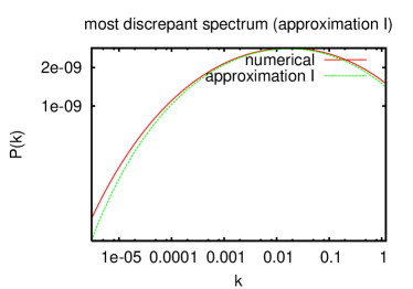
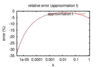
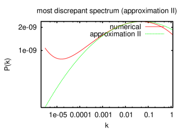
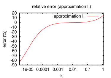
In Figure 3 we plot the most discrepant models in the range, that we call A (for approximation I) and B (for approximation II). The corresponding slow-roll parameters evaluated at the pivot scale are given in Table 3. For approximation II we find a maximum discrepancy in of 83% below , and 19% above (model B). For I, the difference reduces to 33% below and 8% above (model A). So, approximation I is doing better on both sides of the pivot scale.
Indeed, it appears that approximation I captures the spectrum shape very well, but not its amplitude. This is not surprising since in I, the expression for the amplitude is first-order in the slow-roll expansion. The next-order contribution to this approximation should include the parameter , with a positive coefficient. Since the data allows large values of only when is positive, approximation I yields a systematic underestimation of the amplitude. This approach could be straightforwardly improved by computing the curvature amplitude at the next order. In contrast, approximation II tends to give the wrong shape, but since it includes one more order in the slow-roll expansion it can give a better estimate of the amplitude for not too far from .
However, the main result of this section is that the difference between the various spectra is very small, since a large discrepancy is only encountered on scales close to , which have a relatively small statistical weight in the process of accepting or rejecting a model. For both approximations the error in the larger part of the spectrum is of the order of 5%. Current data does not reach such good sensitivity, especially if we keep in mind that for the largest values the curvature spectrum is mainly constrained by the SDSS data, which is always marginalised over an unknown bias parameter. For the particular models shown here, the difference in the effective obtained when fitting either the approximated or the numerical spectrum to the data is for approximation I (model A) and for approximation II (model B). One should keep in mind though, that these are just the most extreme deviations, at the edge of allowed parameter space. On average, the inaccuracies are too small to have a significant effect on the inferred bounds. However, with future datasets one can expect the to become even larger, possibly resulting in biased estimates. Hence, we recommend using the exact numerical approach, since it does not make the analysis longer or more difficult.
The conclusions reached in this section apply to a particular class of inflationary models, namely those described by Eq. (2.3) with parameter ranges limited by current WMAP and SDSS results. Allowing for more freedom in , one would expect stronger deviations between the analytical and numerical approaches. Conversely, imposing a constraint on the total number of -folds for relevant inflation, one would select models which are deeper within slow-roll and obtain even smaller discrepancies. We have limited our discussion to the scalar spectrum, since there is, at present, no evidence for anything but a subdominant tensor contribution in the available data. This may of course change if a primordial -mode polarisation of the CMB is detected in the future.
5 Discussion
We have compared various alternative methods for putting constraints on the observable window of inflationary dynamics, assuming single-field inflation with a smooth behaviour. One could fear that the results would depend very much on the way to compute the spectrum, or on the parameterisation of (i.e., the ensemble of models considered). We point out that with current data these differences are subdominant. The results are mainly affected by the exact prior on the background. By focusing on the allowed window, one hopes to be conservative and to get results dictated by the data only; however these results are very sensitive to the edges of the interval in field space over which accelerated expansion is required. In other words, the upper bound on is given by this constraint rather than the shape of the perturbation spectrum. Current analyses agree with each other, but only within a factor two, due to this difference. This dependence of the final results on the choice of prior may sound worrisome, particularly if it is one’s aim to keep the analysis as general as possible.
It seems as though the priors we initially chose to use with approximations I and II are less restrictive, and would therefore lead to a more conservative result. Unfortunately however, combining these methods with their respective priors on the space of allowed models is fraught with a severe consistency problem. Both priors allow models in regions of parameter space where the approximations are known to break down, and yield results for the spectrum that cannot be trusted. Approximation II, for instance, allows models in which inflation is interrupted within the observable range. Such an event would lead to very distinct signatures, like a cutoff, yet the approximation would still predict a smooth spectrum. It is therefore sensible to expect that inflation lasted at least over the whole observable range. But even that will not be sufficient: if inflation started only just before the observable range, the assumption that the modes start out in the Bunch-Davies vacuum can no longer be justified, and the approximations fail. If, on the other hand, inflation ends just after the smallest observable scale leaves the horizon, the corresponding mode will not have time to freeze out. In fact it would re-enter the horizon right away, and there is no telling (without making further assumptions) in what shape the spectrum would arrive at later times when it is relevant for the determination of the CMB anisotropy spectra.
Hence, it is reasonable to demand a proper vacuum initial condition and a freeze-out of the modes. One could in principle further limit the space of allowed models by constraining the minimum number of -folds before the end of inflation to a certain number, usually taken to be . However, this would require a daring extrapolation of our simple Taylor-expansion over a huge range of -folds, where even a tiny higher derivative of the Hubble parameter would eventually take over. In this paper, therefore, we did not want to make any additional assumptions about what happens after the freeze-out.
There are, however, two points at which the prior of the self-consistent numerical approach is slightly arbitrary, corresponding to the two end points of the interval over which we track the background dynamics. The first one is the large scale end, determined by the time at which we choose the initial conditions for the . We picked as a starting point, but other choices may have been equally good. Fortunately, the data conspire to make this choice have little impact on the final results: only about 0.1% of the models in our chains generated with the laxer prior can be rejected due to inflation starting “too late”.
The more critical issue is the small scale end of the interval. Its choice is connected with the question when a mode can be considered to have frozen out, which is set by the limiting value of at which we stop integrating. The final results for the posterior are mildly dependent on the choice of this limit, which should eventually be chosen such that the resultant uncertainty in the spectra is smaller than the sensitivity of the data. For this reason, we choose here , corresponding to a 0.1% accuracy in the power spectra.
We would like to emphasize once again that the differences in the results are not inherent to the approximations used, but rather due to the attempt to implement them with a minimal prior. Our results also show that if one were to impose a non-minimal prior on the number of -foldings beyond the observable range, the approximations would lead to the same results as the exact method.
In the future, we expect more robust constraints from high-precision experiments, such as, e.g., the Planck satellite. In turn the difference between the various methods for computing the spectra will become even more relevant. In the light of our results, we recommend using the exact numerical approach for a self-consistent analysis of inflationary dynamics.
Acknowledgments
We wish to thank P. Adshead, R. Easther and H. Peiris for very stimulating discussions, and A. Starobinsky for enlightening comments. JH is supported by the ANR (Agence Nationale de la Recherche). WV is supported by the EU 6th Framework Marie Curie Research and Training network “UniverseNet” (MRTN-CT-2006-035863). Numerical simulations were performed on the MUST cluster at LAPP (CNRS & Université de Savoie).
References
References
- [1] Starobinsky A A 1980 Phys. Lett. B91 99–102
- [2] Guth A H 1981 Phys. Rev. D23 347–356
- [3] Sato K 1981 Mon. Not. Roy. Astron. Soc. 195 467–479
- [4] Linde A D 1982 Phys. Lett. B108 389–393
- [5] Albrecht A and Steinhardt P J 1982 Phys. Rev. Lett. 48 1220–1223
- [6] Linde A D 1983 Phys. Lett. B129 177–181
- [7] Starobinsky A A 1979 JETP Lett. 30 682–685
- [8] Mukhanov V F and Chibisov G V 1981 JETP Lett. 33 532–535
- [9] Hawking S W 1982 Phys. Lett. B115 295
- [10] Starobinsky A A 1982 Phys. Lett. B117 175–178
- [11] Guth A H and Pi S Y 1982 Phys. Rev. Lett. 49 1110–1113
- [12] Bardeen J M, Steinhardt P J and Turner M S 1983 Phys. Rev. D28 679
- [13] Abbott L F and Wise M B 1984 Nucl. Phys. B244 541–548
- [14] Peiris H and Easther R 2006 JCAP 0607 002 (Preprint astro-ph/0603587)
- [15] Easther R and Peiris H 2006 JCAP 0609 010 (Preprint astro-ph/0604214)
- [16] Peiris H and Easther R 2006 JCAP 0610 017 (Preprint astro-ph/0609003)
- [17] Lesgourgues J and Valkenburg W 2007 Phys. Rev. D75 123519 (Preprint astro-ph/0703625)
- [18] Lesgourgues J, Starobinsky A A and Valkenburg W 2008 JCAP 0801 010 (Preprint arXiv:0710.1630[astro-ph])
- [19] Martin J and Ringeval C 2006 JCAP 0608 009 (Preprint astro-ph/0605367)
- [20] Covi L, Hamann J, Melchiorri A, Slosar A and Sorbera I 2006 Phys. Rev. D74 083509 (Preprint astro-ph/0606452)
- [21] Ringeval C 2008 Lect. Notes Phys. 738 243–273 (Preprint astro-ph/0703486)
- [22] Lorenz L, Martin J and Ringeval C 2007 (Preprint arXiv:0709.3758[hep-th])
- [23] Powell B A and Kinney W H 2007 JCAP 0708 006 (Preprint arXiv:0706.1982[astro-ph])
- [24] Lewis A, Challinor A and Lasenby A 2000 Astrophys. J. 538 473–476 (Preprint astro-ph/9911177)
- [25] Lewis A and Bridle S 2002 Phys. Rev. D66 103511 (Preprint astro-ph/0205436)
- [26] Liddle A R, Parsons P and Barrow J D 1994 Phys. Rev. D50 7222–7232 (Preprint astro-ph/9408015)
- [27] Kinney W H 2002 Phys. Rev. D66 083508 (Preprint astro-ph/0206032)
- [28] Easther R and Kinney W H 2003 Phys. Rev. D67 043511 (Preprint astro-ph/0210345)
- [29] Mukhanov V F, Feldman H A and Brandenberger R H 1992 Phys. Rept. 215 203–333
- [30] Stewart E D and Lyth D H 1993 Phys. Lett. B302 171–175 (Preprint gr-qc/9302019)
- [31] Leach S M, Liddle A R, Martin J and Schwarz D J 2002 Phys. Rev. D66 023515 (Preprint astro-ph/0202094)
- [32] Leach S M and Liddle A R 2003 Phys. Rev. D68 123508 (Preprint astro-ph/0306305)
- [33] Hinshaw G et al. (WMAP) 2007 Astrophys. J. Suppl. 170 288 (Preprint astro-ph/0603451)
- [34] Page L et al. (WMAP) 2007 Astrophys. J. Suppl. 170 335 (Preprint astro-ph/0603450)
- [35] Montroy T E et al. 2006 Astrophys. J. 647 813 (Preprint astro-ph/0507514)
- [36] Jones W C et al. 2006 Astrophys. J. 647 823 (Preprint astro-ph/0507494)
- [37] Piacentini F et al. 2006 Astrophys. J. 647 833 (Preprint astro-ph/0507507)
- [38] Reichardt C L et al. 2008 (Preprint arXiv:0801.1491[astro-ph])
- [39] Tegmark M et al. 2006 Phys. Rev. D74 123507 (Preprint astro-ph/0608632)
- [40] Malquarti M, Leach S M and Liddle A R 2004 Phys. Rev. D69 063505 (Preprint astro-ph/0310498)
- [41] Makarov A 2005 Phys. Rev. D72 083517 (Preprint astro-ph/0506326)
- [42] Ballesteros G, Casas J A and Espinosa J R 2006 JCAP 0603 001 (Preprint hep-ph/0601134)