Constraining slow-roll inflation with WMAP and 2dF
Abstract
We constrain slow-roll inflationary models using the recent WMAP data combined with data from the VSA, CBI, ACBAR and 2dF experiments. We find the slow-roll parameters to be and . For inflation models we find that at the 2 and levels, indicating that the model is under very strong pressure from observations. We define a convergence criterion to judge the necessity of introducing further power spectrum parameters such as the spectral index and running of the spectral index. This criterion is typically violated by models with large negative running that fit the data, indicating that the running cannot be reliably measured with present data.
pacs:
98.80.Cq astro-ph/0306305I Introduction
The observations by the WMAP satellite wmap1 ; wmapS ; wmapinf ; wmap2 ; wmap3 have brought the global cosmological data set up to a quality where, for the first time, it is possible to obtain precision constraints on cosmological models. That the data provides no indication of any significant departure from gaussianity, adiabaticity, or scale-invariance, and furthermore reveals two coherent peaks in the spectrum of cosmic microwave background (CMB) anisotropies, lends powerful support to the idea of inflation in the early Universe as a source for the observed perturbations. This opens the prospect of constraining and excluding regions of inflation model parameter space.
The qualitative breakthrough of the WMAP data is important. For the first time we have available a CMB spectrum that spans from cosmic variance limited measurements on large angular scales across to the measurement without any overall calibration error of the peaks on small angular scales. Measurements of the polarization of the CMB wmap4 provide some insight into the epoch of reionization which in turn helps to constrain inflationary models by limiting the effects of parameter degeneracies.
In this paper we analyze slow-roll inflation models, following the strategy outlined in Leach et al. LLMS , and provisionally applied to pre-WMAP CMB data by Leach and Liddle infcmb as a demonstration of methodology. With WMAP it is possible to make the first serious application. As compared to our earlier work, we make several improvements. We use the now-ubiquitous Markov Chain Monte Carlo method MCMC ; LB to obtain the likelihood function over parameter space, we include both short-scale CMB data and the galaxy power spectrum data from 2dF (but not any lyman-alpha data, whose inclusion has proven controversial Sel ), and we study the effect of varying one further slow-roll parameter. Our approach differs in several respects from the other papers that have already appeared discussing inflation post-WMAP wmapinf ; BLM ; KKMR , and we contrast our work with theirs in the conclusions.
II Methodology
We follow the methodology described in Refs. LLMS ; infcmb , to which the reader is referred for further details. In terms of the horizon-flow parameters , , etc., the inflationary scalar and tensor power spectra can be well represented as power-laws with amplitude and spectral indices given by SL ; SL2
| (1) | |||||
| (2) | |||||
| (3) |
where . The relative amplitude of tensor and scalar perturbations is given by
| (4) |
Later we will also consider weak running (scale-dependence) of the scalar spectral index. Although the full inflationary predictions are somewhat more detailed, Eqs. (1)–(4) capture the essence of the inflationary power spectra. In the following analysis we start by using the first-order power-law shape predictions for inflation which include the Stewart–Lyth correction to the amplitude, but ignore any term . Later we use the full second-order predictions where the terms are included in the fit.
The data that we use in this paper comes from VSA vsa , CBI cbi , ACBAR acbar , WMAP wmapinf and the 2dF galaxy redshift survey 2df . We compute the microwave anisotropies using the CAMB code LCL coupled to our own slow-roll inflation module LLMS , and use the package CosmoMC LB , modified to include the WMAP likelihood code V , in order to compute the likelihood over parameter space. We generate a Markov chain of 60,000 elements. We assume a flat CDM universe and adopt the parameter basis where and are the baryon and dark matter physical densities, is the Hubble constant, is the amplitude of scalar perturbations, is the redshift of reionization (which is assumed to be instantaneous), and . The only prior that has any effect on the constraints is insisting . We are also interested in the constraints on the derived parameters where is the optical depth to the last scattering surface and .
III The constraints
III.1 Constraints on slow-roll inflation
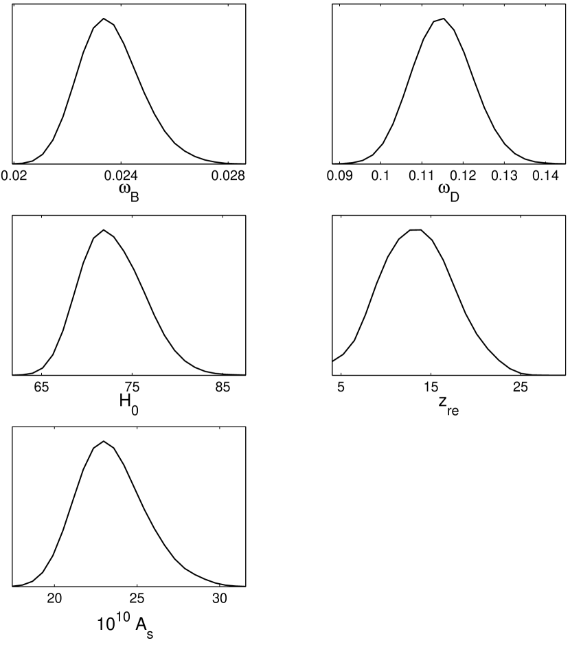
We begin by considering the constraints on slow-roll inflation models, initially only including the horizon-flow parameters and . For orientation and comparison with other work, in Fig. 1 we display the constraints on the basic cosmological parameters . Our results are in good agreement with other authors, unsurprisingly as we use many of the same codes and a similar data compilation.
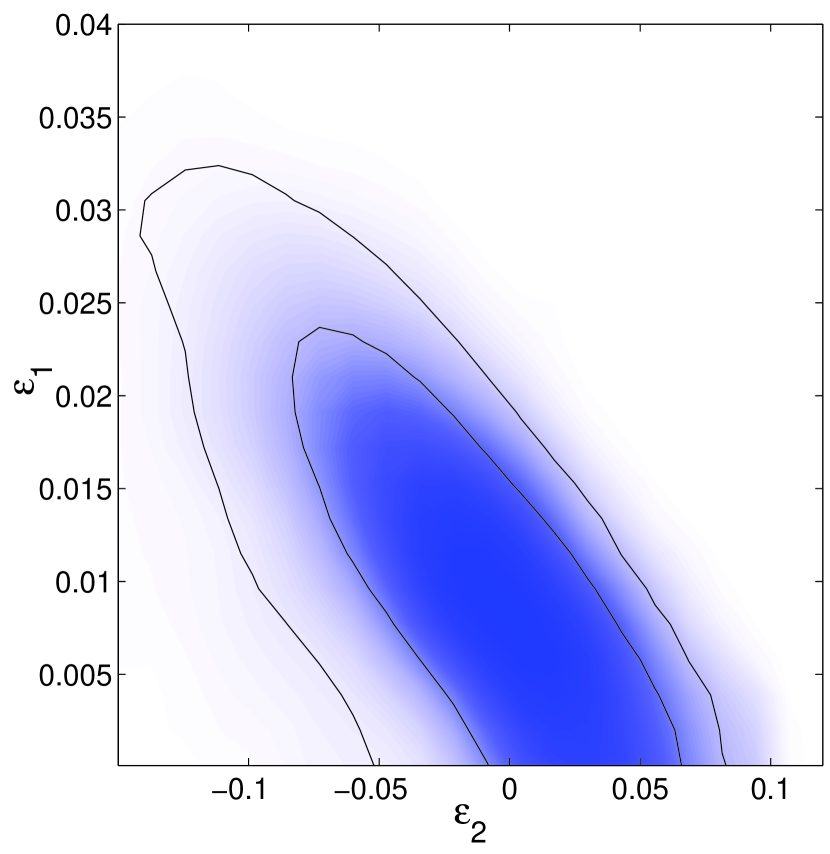
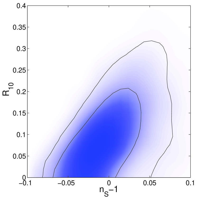
Fig. 2 shows the likelihood distribution in the plane of the horizon-flow parameters and . We can see that the constraint on is highly correlated with , since both parameters contribute to the spectral index. Moreover the data introduce a further degeneracy, the tensor degeneracy. This occurs where models with a tensor component, and hence more power on large scales, require more power to short scales, and hence a bluer spectrum. This is clear from Fig. 3, in which we plot the same constraints in terms of the derived parameters and .
Because of the strong degeneracy between and , we read off the 2 upper limit on from Fig. 2 without marginalizing out , finding
| (5) |
which gives the best measure of the relative (primordial) contribution of tensors, via Eq. (4). This constraint is in agreement with Refs. wmapinf ; BLM . The direct contribution of the tensor spectrum to the spectrum is also of some interest and, similarly, we obtain the 2 upper limit
| (6) |
and using Eq. (1) we obtain an upper limit on the energy scale of inflation
| (7) |
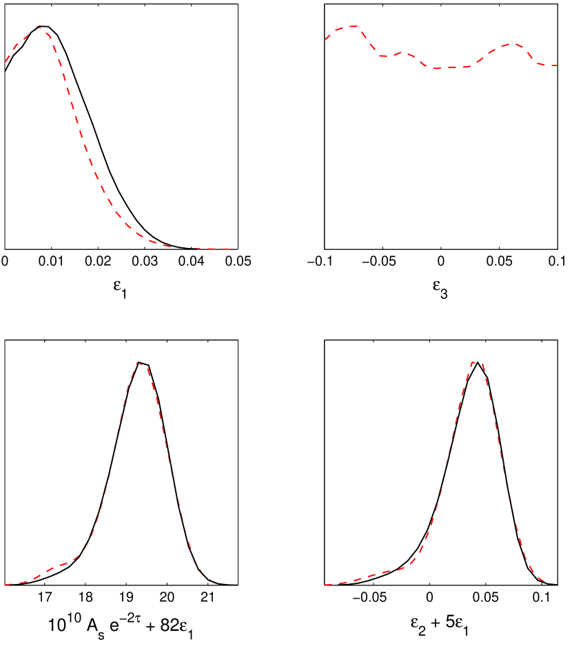
The constraints on the horizon-flow parameters are best summarized in Fig. 2. However, we can define a new parameter along the tensor degeneracy direction and obtain the constraint
| (8) | |||||
| (9) |
and these constraints are displayed in Fig. 4. To obtain constraints on the shape of the inflaton potential we use the slow-roll approximation
| (10) | |||||
| (11) | |||||
| (12) |
and rewriting the constraints Eq. (5)–(8) we find
| (13) | |||||
| (14) | |||||
| (15) |
From these constraints and from Fig. 2, we see that there is no evidence of deviations from the extreme slow-roll limit , which lies comfortably within the contour. The best one can say is that the tensors and tilt can be used to marginally improve the fit to the data.
In comparison with the situation before WMAP (e.g. Ref. infcmb ), the principal change is a considerable tightening of the uncertainties, with the general trend of the shrinking being towards the scale-invariant case. This is sufficient to exclude a significant chunk of slow-roll inflation parameter space. Of the models remaining, there is a mild preference for a red spectral index () but not with any significance. Because of the tight correlation between and there exists a class of models with blue scalar spectra which show a mild preference for a tensor component on large scales, as is visible in Fig 3. This is an area of parameter space which has not been significantly populated with models, as models with blue spectra tend to have negligible tensors. These models have meaning that the fractional kinetic energy of the inflaton is decreasing, which could correspond to models leaving a kinetic energy dominated epoch. These models are also somewhat ‘protected’ by the tensor degeneracy direction and could prove quite resistant to observational pressure for some time to come.
We now ask how well motivated it was to stop at , by including one further horizon-flow parameter . This allows us to include a running (scale-dependence) of the scalar spectral index, given by
| (16) |
and to take the expressions for the spectral indices themselves to second-order SL2 . The effect of including this extra parameter is shown in Fig. 4, where it has a fairly modest effect on the likelihood distributions for other inflationary parameters. However itself is poorly constrained, and is readily consistent with zero. We conclude that there is clearly no motivation to include this extra parameter, with the improved goodness-of-fit being insufficient to warrant its inclusion. We return to this issue in Section IV.2.
III.2 Constraints on power-law inflation
If we have a specific class of inflation models in mind then we can go beyond the constraints of Fig. 2, and in this section we examine the constraints on power-law inflation. This remains an interesting model because the potential, once normalized to the observed perturbation amplitude, is described by a single parameter, and so we can expect tighter constraints than in the case of general slow-roll models. Power-law inflation LM is expansion given by
| (17) | |||||
| (18) |
Equivalently, in terms of conformal time we have
| (19) | |||||
| (20) |
We obtain the constraint on power-law inflation by reading off the 2 bound on at the intersection with the axis and find:
| (21) | |||||
| (22) | |||||
| (23) |
The constraint on is tighter than for slow-roll models because power-law inflation requires a red scalar power spectrum, and so there is no possibility of taking advantage of the tensor degeneracy. If in the near future the HZ spectrum is ruled out in favor of red-tilted spectrum then we can begin to place an upper limit on the index , and needless to say, power-law inflation can be ruled out altogether if a blue-tilted spectrum is favored or if the tensor spectrum has the wrong relationship with the scalar spectrum.
An easy way to overinterpret the data would be to point out that our best-fit models lie close to the region well described by power-law inflation (ie. the axis), with inflationary parameters and . However this is likely to be a result of the mild preference for red scalar spectra combined with a small slide along the (flattish) tensor degeneracy direction once tensors are included in the fit. Nonetheless, it is intriguing that such a simple inflation model should provide such an excellent fit to the data.
III.3 Constraints on monomial inflation
In this section we examine the constraints on monomial inflation potentials of the form
| (24) |
Once normalized to observations these models are defined by two parameters, the index and , the value of when the scale crossed the horizon during inflation. However, there is an extra ingredient: the energy scale of inflation is fixed once we specify and , which is typically around GeV. This in turn specifies the maximum number of -folds of slow-roll inflation after horizon scale crossing, , after which inflation must end (regardless of the mechanism that ends inflation) giving way to reheating and the standard expansion history SD ; efolds . In addition, monomial inflation provides a mechanism to end inflation via the violation of slow-roll, and so we can calculate the functions , , and where is the number of -folds from the end of inflation. This allows us to map a constraint on to a constraint on the slow-roll parameters.
Substitution of the potential of Eq. (24) into Eq. (11) and (12) gives
| (25) | |||||
| (26) |
We can calculate the number of -folds of inflation from the definition
| (27) | |||||
| (28) |
where is the initial value of . Using , which is a good approximation for monomial inflation, we have
| (29) |
and in the limit the horizon flow parameters are given by
| (30) | |||||
| (31) |
Eq. (31) gives us the useful constraint
| (32) |
where is the number of -foldings from the end of inflation that the scale crossed the horizon (in the language of Ref. efolds , ). It should be emphasized that the specific form of this constraint applies only for the monomial potentials. The maximum number of -folds of slow-roll inflation corresponding to our scale is approximately 60 SD ; efolds and so we have the constraint . Using this additional constraint we can rule out certain monomial inflation models independent of the actual number of -folds of slow-roll inflation after horizon scale crossing.
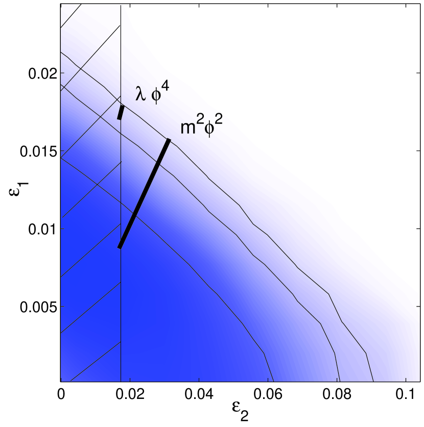
In Fig. 5, which is a zoom of part of Fig. 2, we restrict our attention to which corresponds to models where the ratio between the scalar field kinetic and total energy density is increasing, arguably the most natural candidates for ending inflation by the violation of slow-roll. The solid lines show the location of the quadratic and quartic potential models at different numbers of -foldings up to the maximum. The quartic potential lies outside the contour for any allowed value of .
We can constrain the exponent by reading off the value of at the point where the observational constraints on the slow-roll parameters intersect with the constraint on given by Eq. (32). We find the monomial inflation index is constrained from above to be
| (33) |
Thus, while it is still too early to definitively rule out the inflation model, it is clear from the pattern of the above constraints that this particular model is under very strong pressure from observations. The is valid as long as (note that monomial inflation models with must have a prolonged reheating epoch at the end of inflation or non-standard post-inflationary evolution efolds ). It is clear from Fig. 5 that the same kind of pressure will build on the model if the spectral index becomes more tightly constrained, since lines of constant spectral index correspond to , which, modulo the tensor degeneracy, runs parallel to the constraint contours.
It is natural to ask what can we say in a model-independent manner about slow-roll inflation models while still including the bound on . The number of -folds of inflation, given by Eq. (28), depends only on the function , and this gives us a straightforward way to study the phenomenology of inflation models. Unfortunately, we only have information about the function across the 8 or so -folds across observable scales, and so the rest of this function can be at best extrapolated from observable scales. The initial slope is given by
| (34) |
and so the higher slow-roll parameters, via the running of the spectral index Eq. (16), would contain useful additional information about the model of inflation, assuming inflation occurs at these high energies. Since we have found no constraint on , then it is clear that we can not make this type of model independent analysis at present. Note also that the bound can be relaxed somewhat to if is significantly reduced in the late stages of inflation efolds . In terms of the slow-roll parameters
| (35) |
For instance, this correction is relevant for the which has , although this is certainly not enough to take much pressure off this model.
IV Discussion
IV.1 The Harrison–Zel’dovich spectrum
We have discounted the inclusion of because the data are unable to distinguish it from zero. However, following the logic of that statement we are forced to conclude that neither nor have been shown to be inconsistent with zero. The minimal assumption concerning the data is in fact that it is due to a Harrison–Zel’dovich (HZ) spectrum, with no indication of inflationary dynamics.
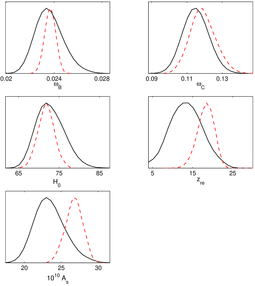
It is plausible therefore to also regard and as giving poor value, in terms of the improvement to the fit they give, for their inclusion as extra parameters. It is therefore interesting to see how constraints tighten up if we assume an HZ spectrum in place of slow-roll inflation. In Fig. 6 we display once more the constraints on the basic cosmological parameters, but now also showing the constraints assuming the HZ spectrum and no tensors. It is clear that, broadly speaking, the two models are in good agreement with each other, but nevertheless there are quantitative differences worth remarking upon. The baryon density becomes much more tightly constrained, and looks rather high when compared to nucleosynthesis constraints. Perhaps most interestingly, assuming HZ the constraints on the reionization epoch tighten considerably in favour of early reionization, as in abandoning slow-roll we have lost the ability to use tilt and tensors to partially mimic the effects of reionization.
IV.2 A convergence criterion
As long as the HZ model remains a good fit to the data then the issue of introducing the spectral index as a parameter, let alone the running of the spectral index, needs some consideration. Reconstructing the initial power spectrum in bands BLWE ; MW indicates that it is adequately fit by a scale-invariant spectrum, and that there should be nothing to be gained by adding any further power spectrum parameters. Indeed, why do we include further power spectrum parameters at all? If we consider the power spectrum as a Taylor expansion
| (36) | |||||
then the primary reason for including higher power spectrum parameters is to the test the convergence of the observable, in this case , as described at lower-order. The first term in the series has been determined to be . We can introduce the next order parameter, the spectral index, without disrupting the constraints on the other parameters, and moreover feel confident of our measurement of , provided
| (37) |
The above criterion is indeed satisfied by all the models under consideration since and . Thus the determination of the amplitude of scalar perturbations to a reasonable accuracy is not questioned by anybody. Similarly, one can feel confident in a measurement of if the criterion
| (38) |
is satisfied, and the fact that this inequality is typically violated for many of the strong running models under consideration in the literature (eg. the best fit of Ref. wmapS is , and the two terms are of the same order of magnitude) has two possible explanations. The first is the intriguing possibility that the third term in the Taylor expansion Eq. (36) dominates over the second term at around a scale of , physically corresponding to a power spectrum with a maximum near . This can only be verified if the contribution to the power spectrum from the fourth term (the running of the running) is found to be less than the term due to the running itself at this scale. The second, and more likely, explanation is that the large allowed variation in the running of the spectral index is just a symptom of the fact that we haven’t convincingly determined the spectral index yet. We suggest that this criterion can be easily used as a check in the fitting procedure: if Eq. (38) is violated for most models and the running is detected only at low significance, then the simplest interpretation is that no useful information is coming from the inclusion of the new parameter in the fit. One should at least be aware of a lack of convergence in the power spectrum observable, Eq. (36).
Alternatively, one can think of Eq. (38) as setting the boundary between weak and strong running in an observational sense. For current observations weak running is given by models with , and this can be useful one wishes to introduce a weak running prior into the fitting procedure as a perturbation analysis to the existing constraints.
This type of convergence criterion should find echoes in other areas of cosmology where an observable is in some way series expanded, for instance the dark energy equation of state HT .
Before concluding, we bring together the cosmological parameters of various inflationary models in Table 1. The models have been selected by fixing their values of and , and where a chain was not already available we have run a short chain to determine reasonable values for the other parameters. These models may be useful as fiducial parameters for future study and, being within the 1 contour of Fig. 2, they are approximately degenerate at the level of the current data set.
| BF | 0.023 | 0.117 | 71.3 | 13.1 | 23.4 | 0.008 | -0.0007 | 0.98 | 0.07 |
| BFT | 0.022 | 0.115 | 70.5 | 15.0 | 24.1 | 0 | 0.03 | 0.97 | 0 |
| BFHZ | 0.024 | 0.119 | 71.9 | 18.5 | 26.8 | 0 | 0 | 1 | 0 |
| 0.022 | 0.107 | 71.5 | 7.1 | 20.3 | 0.017 | 0.017 | 0.95 | 0.13 | |
| 0.023 | 0.114 | 70.9 | 10.5 | 22.1 | 0.008 | 0.017 | 0.97 | 0.06 | |
| TD1 | 0.025 | 0.107 | 77.4 | 15.0 | 23.0 | 0.023 | -0.077 | 1.03 | 0.21 |
| B1 | 0.025 | 0.113 | 76.7 | 17.2 | 24.7 | 0.018 | -0.077 | 1.04 | 0.16 |
V Conclusions
We have investigated the constraints on various slow-roll inflationary models coming from observations of the CMB and large-scale structure. The main result is that the viable slow-roll parameter space is dramatically reduced and the underlying inflationary degeneracy now becomes visible. Interestingly, if we combine these constraints with a constraint on the number of -folds of inflation since horizon scale crossing, then we find that the inflation model is under strong pressure, though not yet definitively ruled out. The model will come under the same threat as long as the data continue to favour the Harrison-Zel’dovich spectrum.
We also introduced a simple convergence criterion, Eq. (38), to judge the necessity of including higher power spectrum parameters such as the spectral index and the running of the spectral index. Applying this criterion we find that while it is justified to include the spectral index in the fit (reflecting the fact that amplitude of scalar perturbations is now well determined), it is not useful to include the running of the spectral index at present.
Our inflation analysis comes after those of Refs. wmapinf ; BLM ; KKMR , with whom we find general agreement. We can make the most direct comparison with Barger et al. BLM , who used the WMAP data alone with a top-hat prior, and a grid based maximization procedure to obtain their constraints. We have have found tighter constraints using WMAP, VSA, CBI, ACBAR, 2dF datasets, and an MCMC technique, with our 2 constraint in Fig. 2 being only slightly looser than their equivalent 1 constraint. The comparison with Peiris et al. wmapinf is less straightforward, since we did not consider the effect of strong running of the spectral index, arguing in Sec. IV.2 that we can obtain better value from the current data set without it. As a result, their results marginally favour a model with a blue scalar spectrum on the largest scales (even in the tensorless limit), whereas the power-law fits in the literature, including their adiabatic/isocurvature fit, favour a slightly red spectrum. Both Peiris et al. and Kinney et al. KKMR investigate the Monte-Carlo flow reconstruction technique, which inevitably involves an extrapolation of the inflationary potential and physics well beyond the region directly constrained by observations. Therefore a certain caution is required when interpreting those analyses. We have hinted in Sec. III.3 how one might make such an extrapolation of the horizon-flow parameters (instead of the potential), but the method would require considerably tighter constraints on the running of the spectral index than we have at present.
Acknowledgements.
S.M.L is supported by the EU CMBNET network, and A.R.L. in part by the Leverhulme Trust. We thank Dominik Schwarz, Ruth Durrer, Roberto Trotta, and Michaël Malquarti for useful discussions.References
- (1) C. L. Bennett et al., astro-ph/0302207.
- (2) D. N. Spergel et al., astro-ph/0302209.
- (3) H. V. Peiris et al., astro-ph/0302225.
- (4) E. Komatsu et al., astro-ph/0302223.
- (5) G. Hinshaw et al., astro-ph/0302217.
- (6) A. Kogut et al., astro-ph/0302213.
- (7) S. M. Leach, A. R. Liddle, J. Martin, and D. Schwarz, Phys. Rev. D66 023515 (2002), astro-ph/0202094.
- (8) S. M. Leach and A. R. Liddle, Mon. Not. Roy. Astr. Soc. 341 1151, (2003), astro-ph/0207213.
- (9) N. Christensen and R. Meyer, astro-ph/0006401; N. Christensen, R. Meyer, L. Knox, and B. Luey, Class. Quant. Grav. 18, 2677 (2001), astro-ph/0103134.
- (10) A. Lewis and S. Bridle, Phys. Rev. D66, 103511 (2002), astro-ph/0205436.
- (11) U. Seljak, P. MacDonald, and A. Makarov, astro-ph/0302571.
- (12) V. Barger, H. Lee, and D. Marfatia, hep-ph/0302150.
- (13) W. H. Kinney, E. W. Kolb, A. Melchiorri, and A. Riotto, hep-ph/0305130.
- (14) V. F. Mukhanov and G. V. Chibisov, JETP Letters, 33, 532 (1981), astro-ph/0303077; V. F. Mukhanov, H. A. Feldman, and R. H. Brandenberger, Phys. Rep. 215, 203 (1992).
- (15) E. D. Stewart and D. H. Lyth, Phys. Lett. B, 302, 171 (1993), gr-qc/9302019.
- (16) K. Grainge, et al., astro-ph/0212495.
- (17) T. J. Pearson et al., astro-ph/0205388.
- (18) C. L. Kuo et al., astro-ph/0212289.
- (19) W. J. Percival et al., Mon. Not. Roy. Astr. Soc. 327, 1297 (2001), astro-ph/0105252.
- (20) A. Lewis, A. Challinor, and A. Lasenby, Astrophys. J. 538, 473 (2000), astro-ph/9911177.
- (21) L. Verde et al., astro-ph/0302218.
- (22) F. Lucchin and S. Matarrese, Phys. Rev. D 32, 1316 (1985).
- (23) S. Dodelson and L. Hui, astro-ph/0305113.
- (24) A. R. Liddle and S. M. Leach, astro-ph/0305263.
- (25) S. L. Bridle, A. M. Lewis, J. Weller, and G. Efstathiou, astro-ph/0302306.
- (26) P. Mukherjee and Y. Wang, astro-ph/0303211.
- (27) D. Huterer and M. S. Turner, AIP Conf. Proc. 599, 140 (2001) astro/ph 0006419; I. Maor, R. Brustein, and P. J. Steinhardt, Phys. Rev. Lett. 86, 6 (2001), Erratum-ibid. 87, 049901 (2001) astro-ph/0007297; J. Weller and A. Albrecht, Phys. Rev. D65,103512 (2002) 103512, astro-ph/0106079 7222 (1994), astro-ph/9408015.