A measurement of the polarization-temperature
angular cross power spectrum of the Cosmic Microwave Background
from the 2003 flight of BOOMERANG

Abstract

We present a measurement of the temperature-polarization angular cross power spectrum, $\langle TE\rangle$, of the Cosmic Microwave Background. The result is based on $\sim 200$ hours of data from 8 polarization sensitive bolometers operating at 145 GHz during the 2003 flight of Boomerang. We detect a significant $\langle TE\rangle$ correlation in the $\ell$-range between 50 and 950 with a statistical significance $>3.5~{}\sigma$. Contamination by polarized foreground emission and systematic effects are negligible in comparison with statistical uncertainty. The spectrum is consistent with previous detections and with the “concordance model” that assumes adiabatic initial conditions. This is the first measurement of $\langle TE\rangle$ using bolometric detectors.

1. Introduction

Since Rees pioneering work (Rees, 1968), polarization of the Cosmic Microwave Background (cmb) has been at the center of several theoretical studies.

Detailed numerical predictions have been made in the framework of standard inflationary models with primordial adiabatic and scale-invariant fluctuations (see e.g. Bond & Efstathiou, 1984; Seljak & Zaldarriaga, 1996). cmb polarization data is highly useful for cosmology since it can shed light, for example, on the process of reionization of the intergalactic medium (see e.g. Efstathiou, 1988; Zaldarriaga, 1997), on the amplitude of the inflationary gravity waves background (Crittenden et al., 1995; Zaldarriaga & Seljak, 1997; Kamionkowski et al., 1997) and on the nature of primordial perturbations (see e.g. Spergel & Zaldarriaga, 1997; Bucher et al., 2001). Moreover, polarization can provide further evidence for coherent acoustic oscillations in the early universe, since in this case peaks in the temperature and polarization power spectra are expected to be 180 degrees out of phase (Kosowsky, 1998). Unfortunately, given the small amplitude of the signal, current cmb polarization data, while providing an important confirmation of the standard scenario, are unable to provide useful constraints on the parameters of the model. As first suggested in Coulson et al. (1994), measuring the temperature-polarization cross correlation is easier, since the signal is higher and carries most of the cosmological information present in the polarization data.

Previous detections of the temperature-polarization angular cross power spectrum have been obtained by the WMAP satellite (Kogut et al., 2003) and by the DASI (Kovac et al., 2002; Leitch et al., 2004) and CBI (Readhead et al., 2004) interferometers.

In this paper we present new observations of the temperature-polarization cross power spectrum of the Cosmic Microwave Background anisotropy obtained by the Boomerang experiment flown in Jan. 2003 (B03). Results on the temperature and polarization power spectra alone are presented in two companion papers (Jones et al., 2005; Montroy et al., 2005); the instrument and the analysis pipeline producing the maps of temperature and polarization are described in Masi et al. (2005); the cosmological parameter extraction is in MacTavish et al. (2005).

In the present paper we will follow the notation of Zaldarriaga & Seljak (1997) (but see also Kamionkowski et al., 1997) in which polarization is expressed as two linear combinations of spin$\pm 2$ multipole moments which have opposite parities, the so-called $E$ (electric) and $B$ (magnetic) modes. In standard cosmological models, the magnetic-type parity combination does not cross-correlate with temperature or the electric-type parity combination. The cosmological information in the polarization-temperature correlation is therefore present only in the $\langle TE\rangle$ angular power spectrum. In this paper we will also present constraints on $\langle TB\rangle$ as useful check for systematics and foregrounds. Non zero $\langle TB\rangle$ may also appear in exotic theories due for example to the presence of helical flows in the primordial plasma at the time of recombination (Pogosian et al., 2002).

We have performed the analysis of the B03 data using two completely independent pipelines, with different procedures for the pointing solution, data cleaning, deconvolution, map-making and noise estimation, and different estimation of the calibration factors, beams, receivers transfer functions, polarization efficiencies and polarizer angles. One pipeline was developed in Italy (IT), the other in North America (NA). Pipelines details are in Masi et al. (2005) and will be described furthermore in subsequent papers. The most important result from this splitting is the overall agreement, which enhances confidence in the result. A comparison of the result from the two pipelines allows a measure of the sensitivity of the result to details of the analysis.

2. $\langle TE\rangle$ estimation

We use data from 8 channels at 145 GHz, composed of 4 pairs of Polarization Sensitive Bolometers (PSB)- (W1, W2), (X1, X2), (Y1,Y2) and (Z1, Z2), with effective angular resolution of 11.5 arcminutes (full width half maximum, including pointing jitter). Performance and characteristics of those devices are in Masi et al. (2005), together with the full description of the instrument and of the temperature and polarization maps that are used for the analysis presented here.

With polarization sensitive bolometers Boomerang produces maps of the three Stokes parameters, $I$, that describe fluctuations in the brightness of the radiation, $Q$ and $U$ that describe the linear polarization. The intensity of the cmb is conveniently described in terms of temperature fluctuations $\Delta T$ of a black-body respect to a 2.725 Kelvin black-body, and can be decomposed in spherical harmonics as $\Delta T(\hat{n})=\sum_{\ell m}a^{T}_{\ell m}Y_{\ell m}(\hat{n})$. Similarly the linear polarization $Q+iU$ is decomposed using the spin-2 weighted basis ${}_{\pm 2}Y_{\ell m}$

$$(Q\pm iU)(\hat{n})=\sum_{\ell m}\left(a_{\ell m}^{E}\mp ia_{\ell m}^{B}\right)~{}_{\pm 2}Y_{\ell m}(\hat{n})$$ (1)

thus defining the scalar field $E(\hat{n})=\sum_{\ell m}a^{E}_{\ell m}Y_{\ell m}(\hat{n})$ and the pseudo-scalar $B(\hat{n})=\sum_{\ell m}a^{B}_{\ell m}Y_{\ell m}(\hat{n})$. In the hypothesis that those quantities are Gaussian distributed and that the early Universe is isotropic, the cosmological information is encoded in the standard deviations and correlations of the coefficients:

$$\langle XY\rangle=\langle a^{X*}_{\ell m}a^{Y}_{\ell^{\prime}m^{\prime}}\rangle=C_{\ell}^{XY}\delta_{\ell\ell^{\prime}}\delta_{mm^{\prime}}$$ (2)

where the pairs $\langle XY\rangle$ can be $\langle TT\rangle$, $\langle EE\rangle$, $\langle BB\rangle$, $\langle TE\rangle$, $\langle TB\rangle$ and $\langle EB\rangle$. Given the isotropy, these power spectra can be estimated by averaging over $m$ at each multipole number $\ell$.

Both IT and NA power spectra estimation pipelines are based on the MASTER method (Hivon et al., 2002) that computes the pseudo-$a_{\ell m}$ on a fraction of the sphere defined by the function $W(\hat{n})$ that takes into account weighting and sky coverage. This yields the definition of mode-mode coupling kernels that depend only on the weighted scheme. Using an appropriate $\ell$-binning it is possible to solve for the underlying angular power spectra, taking into account the binning operator, the angular resolution of the instrument, the pixelization, and the filtering of time stream. The quantity that is normally used for the binning is the flattened power spectrum $\mathcal{C}_{\ell}=\ell(\ell+1)C_{\ell}/2\pi$. For a set of $n$ bins indexed by $b$, with boundaries $\ell_{\rm{low}}^{(b)}<\ell_{\rm{high}}^{(b)}<\ell_{\rm{low}}^{(b+1)}$, the binning operator is defined as

$$P_{\ell}^{b}=\cases{\frac{1}{\ell_{\rm{low}}^{b+1}-{\ell_{\rm{low}}^{b}}}&if $2\leq\ell_{\rm{low}}^{(b)}\leq\ell\leq\ell_{\rm{low}}^{(b+1)}$\cr 0&otherwise.\cr}$$ (3)

and the power in each bin (hereafter band powers) are $\mathcal{C}_{b}=P_{\ell}^{b}\mathcal{C}_{\ell}$.

The method is based on Monte Carlo simulations of signal-only time-streams, from simulations of the cmb, and of noise-only time-streams, from simulations of the instrument. Both simulated data-streams are processed in the same way as the real data, in order to take into account the overall effect of data filtering and partial sky coverage, and to estimate the noise bias to be removed in the power spectra estimation.

The signal simulations are obtained from random realization of the cmb sky, in temperature and polarization, given an underlying cosmological model, projected in a time stream according to the Boomerang pointing solution. The noise simulations are obtained from random realization of the noise power spectrum, iteratively estimated, taking into account noise correlation between channels as described in Masi et al. (2005).

The covariance matrix ${\bf M}_{bb^{\prime}}$, that defines the uncertainties in the $\mathcal{C}_{b}$ determination, is estimated by Monte Carlo simulations of signal plus noise as in Hivon et al. (2002). An approximation of the diagonal part of this matrix is given by

$$\sigma^{2}_{TE,b}= {{2}\over{(2\ell_{b}+1)f_{\rm{sky}}\Delta\ell}}$$

$$\left[\mathcal{C}^{2}_{TE,b}+\left(\mathcal{C}_{T,b}+{{\mathcal{N}_{T,b}}\over{B_{b}}^{2}}\right)\left(\mathcal{C}_{E,b}+{{\mathcal{N}_{E,b}}\over{B_{b}}^{2}}\right)\right]$$

where $f_{\rm{sky}}$ is the effective observed fraction of sky, $\mathcal{C}_{T,b}$, $\mathcal{C}_{E,b}$ and $\mathcal{C}_{TE,b}$ are the band powers of the temperature, the polarization and the polarization-temperature correlation respectively, $\mathcal{N}_{T,b}$ and $\mathcal{N}_{E,b}$ are the band powers of the noise in the temperature map and in the $E$ map, $B_{b}$ is the spherical harmonic transform of the beam, and $\Delta\ell$ is the bin width.

2.1. Weighting

The last flight of Boomerang, described in Masi et al. (2005), was split into three parts: a deep observation over 0.22% of the sky, centered at $RA=82.5^{\circ}$, $DEC=-45^{\circ}$ (hereafter deep region), a shallow observation on a region of covering the 1.8% of the sky (including the deep region) centered in the same coordinates (hereafter shallow region), and observation of the Galactic plane that is not used in these power spectra analysis. Wide coverage and deep integration are both important for the quality of the result. The wide coverage of the shallow region is useful to reduce sample variance, the deep integration of the deep region to reduces the statistical noise.

The two pipelines use different methods to combine the data to obtain a compromise of sample variance and noise. In the NA pipeline we perform independent analysis of the shallow scans and of the deep scans, computing the respective $a_{\ell m}^{T}$ and $a_{\ell m}^{E}$. We then estimate four $\langle TE\rangle$ cross spectra, $\langle T_{s}E_{s}\rangle$, $\langle T_{s}E_{d}\rangle$, $\langle T_{d}E_{s}\rangle$, $\langle T_{d}E_{d}\rangle$, with the relative correlation matrices and combine the spectra appropriately (C.R. Contaldi, in preparation). In the IT pipeline, a single map with all the scans is used. The $a_{\ell m}^{T}$ are computed on the shallow region, the $a_{\ell m}^{E}$ on the deep. The effect of such a double coverage is taken into account in the transfer function and kernel used to derive the $\langle TE\rangle$ spectrum.

2.2. Result and significance

Table 1 Boomerang-03 Temperature-polarization cross power spectra band powers.

	NA				IT
$\ell_{b}$	$\mathcal{C}_{b}^{TE}$	$\Delta\mathcal{C}_{b}^{TE}$	$\mathcal{C}_{b}^{TB}$	$\Delta\mathcal{C}_{b}^{TB}$	$\mathcal{C}_{b}^{TE}$	$\Delta\mathcal{C}_{b}^{TE}$	$\mathcal{C}_{b}^{TB}$	$\Delta\mathcal{C}_{b}^{TB}$
51	22	32	2	33	-9	51	2	51
150	-51	27	-18	27	-71	39	-68	37
250	40	32	-9	31	125	46	-73	42
350	58	28	-16	27	63	34	29	30
450	-90	29	7	28	-69	40	-17	36
550	40	39	-2	35	20	44	66	39
650	-18	45	-2	42	-8	65	91	60
750	-86	60	-88	58	-88	56	65	51
850	62	74	74	72	77	86	69	82
950	-61	90	-70	88	-115	72	199	65
1500	48	81	-133	81	90	105	-12	100

Figure 1.— The $\langle TE\rangle$ power spectrum band powers for the NA (filled circles) and IT (open circles) pipelines. The upper part of the plot reports data with errorbars, the fiducial model ($\Lambda$CDM model fit to WMAP (year 1), Acbar, and CBI) as a black curve and the binned fiducial model as histogram. The middle and bottom plots are the results of two different consistency tests, obtained splitting the data in channels (WX-YZ) and in time (half 2 - half 1) respectively. In the low-$\ell$ part of the plot is evident the effect of a different weighting scheme between IT and NA, while at large multipoles the result is dominated by the same instrumental performances.

Figure 2.— The $\langle TB\rangle$ power spectrum band powers for the NA (filled circles) and IT (open circles) pipelines. The upper part of the plot reports the $\langle TB\rangle$ data with error-bars. The middle and bottom plots are the results of two different consistency tests, obtained splitting the data in channels (WX-YZ) and in time (half 2 - half 1) respectively.

Figure 3.— Likelihood of the parameters $a$ and $\Delta\ell$. Parameter $a$ is defined as the amplitude of the $\langle TE\rangle$ fiducial model, $\Delta\ell$ is the shift in multipole $\ell$ applied to the $\langle TE\rangle$ fiducial model. The continuum lines are for the Boomerang $\langle TE\rangle$ data, the dashed lines are for $\langle TB\rangle$ data, compared to the same $\langle TE\rangle$ fiducial model. In the central plot is reported the two dimensional likelihood, $\mathcal{L}(\Delta\ell,a)$; the contours are 1, 2, and 3 $\sigma$, corresponding to 68.3, 95.4 and 99.7% of probability. The $\times$ symbol is the expected value for $\langle TE\rangle$ given the fiducial model, the + symbol is the expected value for $\langle TB\rangle$. In the right plot is reported the $\mathcal{L}(a)$ marginalizing over $\Delta\ell$, and in the top plot, the $\mathcal{L}(\Delta\ell)$ marginalizing over $a$. In the right and top plot, the gray lines are 1, 2, and 3 $\sigma$ boundaries for the $\langle TE\rangle$ data. The $\langle TB\rangle$ data likelihood is used to test the presence of foregrounds and systematic effects that would affect $\langle TE\rangle$ and $\langle TB\rangle$ in the same way. This plot is obtained using the IT dataset with a binning width of 50 multipole numbers. The NA dataset gives a similar result.

Table 2$\langle TE\rangle$ and $\langle TB\rangle$ statistics

	Test	d.o.f.	$\chi^{2}$	$\Lambda$	PTE	$\sigma_{\mbox{reject.}}$
NA	$\langle TE\rangle$ compared to fiducial	9	5.81	0.48	0.62
	$\langle TE\rangle$ compared to zero	9	23.1	8.23	$2.6\times 10^{-4}$	3.5
	$\langle TB\rangle$ compared to zero	9	4.94	0.08	0.92
	$\langle TB\rangle$ compared to fiducial $\langle TE\rangle$	9	24.9	10.5	$2.9\times 10^{-5}$	4.0
IT	$\langle TE\rangle$ compared to fiducial	9	4.59	1.83	0.26
	$\langle TE\rangle$ compared to zero	9	20.8	11.3	$1.2\times 10^{-5}$	4.2
	$\langle TB\rangle$ compared to zero	9	15.1	1.86	0.16
	$\langle TB\rangle$ compared to fiducial $\langle TE\rangle$	9	34.5	20.7	$1.0\times 10^{-9}$	6.0

Note. — Significance of the $\langle TE\rangle$ and $\langle TB\rangle$ results respect to models. The first bin is not used in this analysis since it can be contaminated by instrumental effects.

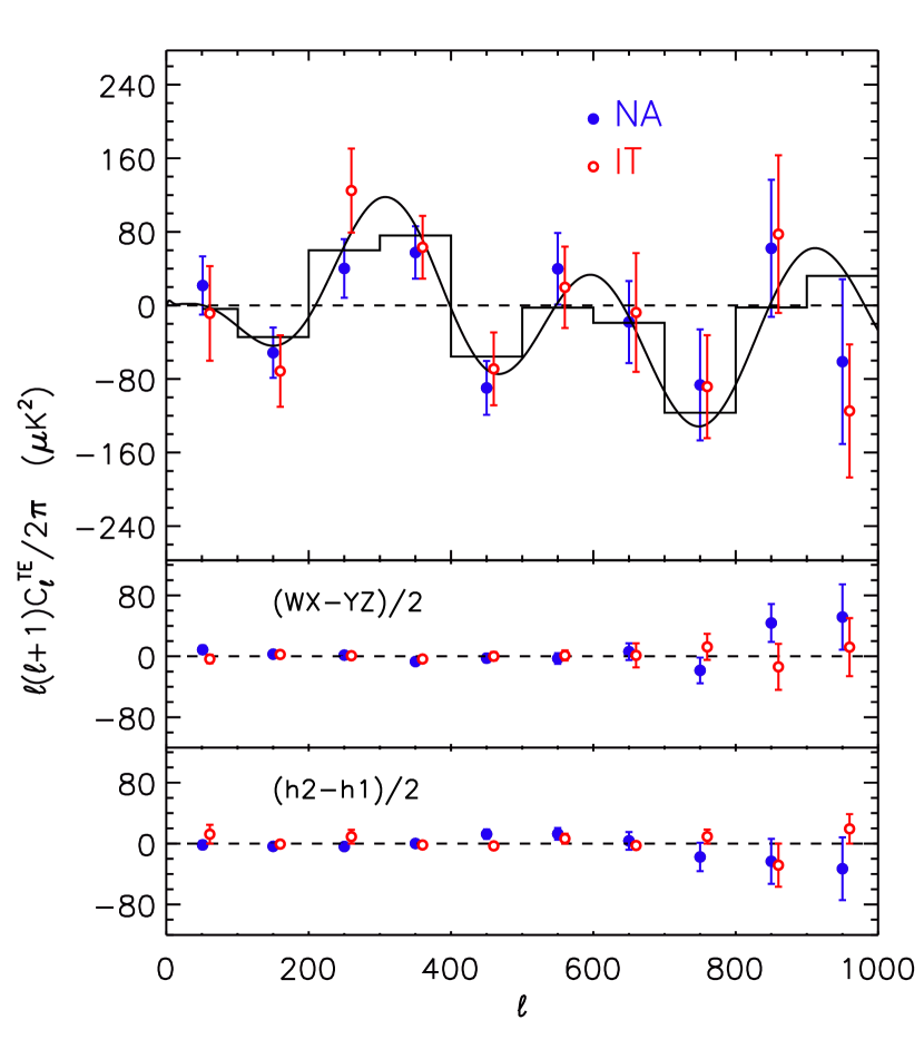
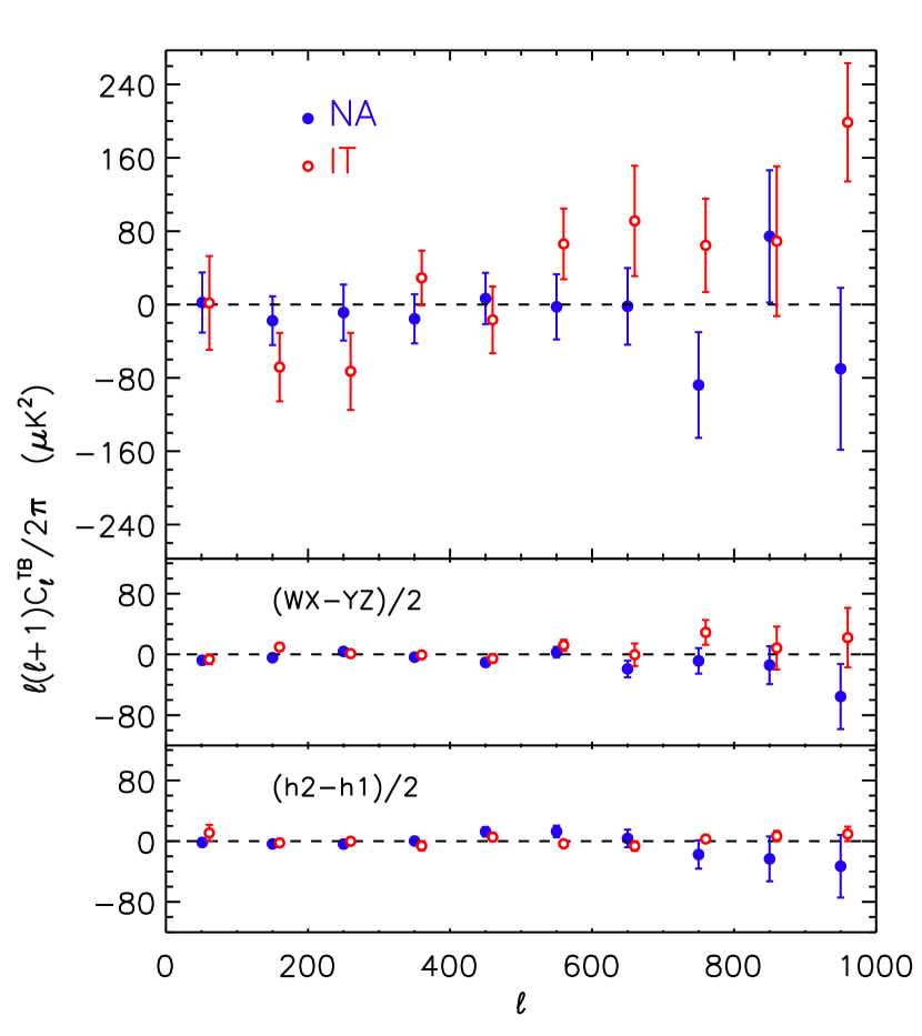
The results for the $\langle TE\rangle$ and $\langle TB\rangle$ power spectra are reported in the upper panel of Figures 1 and 2 respectively and in Table 1.

Both pipelines assume a flat shape for the power in each band (see equation 3). For comparison with model band powers, the IT pipeline assumes flat band power window functions while the NA pipeline computes from the Xfaster fisher matrix estimator the band power window functions $\mathcal{W}_{\ell}^{b}$, that are used, in place of $P_{\ell}^{b}$, to convert a model power spectra $\mathcal{C}_{\ell}^{\rm{mod}}=\ell(\ell+1)C_{\ell}^{\rm{mod}}/2\pi$ into the theoretical band powers as

$$\mathcal{C}_{b}^{\rm{mod}}=\frac{\mathcal{I}\left[\mathcal{W}_{\ell}^{b}\mathcal{C}_{\ell}^{\rm{mod}}\right]}{\mathcal{I}\left[\mathcal{W}_{\ell}^{b}\right]}$$ (5)

where $\mathcal{I}\left[f_{\ell}\right]=\sum_{\ell}\frac{\ell+\frac{1}{2}}{\ell(\ell+1)}f_{\ell}$ is the logarithmic integral defined in Bond et al. (2000). Band powers, covariance matrices and window functions are available at the Boomerang web-pages.

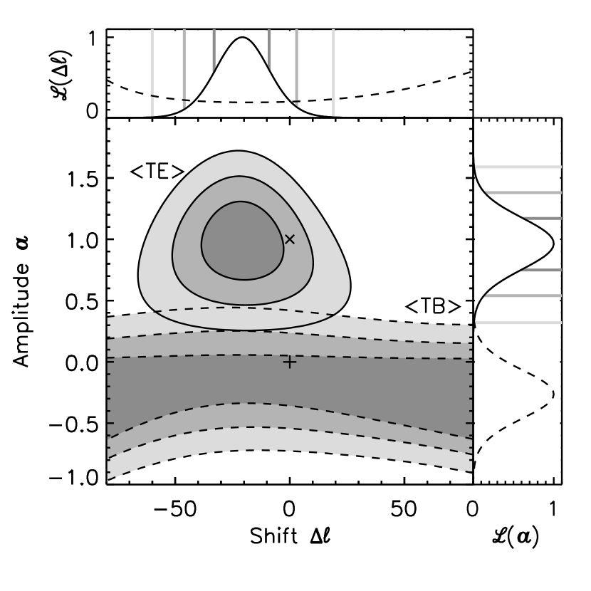
To quantify the agreement of the detection with standard cosmology, we compare the result to $\mathcal{C}_{b}^{\rm{mod}}$, the theoretical band powers of a fiducial model given by the $\Lambda$CDM model of Spergel et al. (2003) fit to WMAP (year 1), Acbar, and CBI, which we scale by a factor $a$ and shift by $\Delta\ell$. We compute the two dimensional likelihood as

$$\mathcal{L}(a,\Delta\ell)\propto$$ (6)

$$\exp\left(-{1\over 2}\sum_{bb^{\prime}}\left(\mathcal{C}_{b}-a\cdot\mathcal{C}_{b,\Delta\ell}^{\rm{mod}}\right){\bf M}_{bb^{\prime}}^{-1}\left(\mathcal{C}_{b^{\prime}}-a\cdot\mathcal{C}_{b^{\prime},\Delta\ell}^{\rm{mod}}\right)\right)$$

where $\mathcal{C}_{b^{\prime},\Delta\ell}$ are the band powers after shifting by $\Delta\ell$ the power spectrum. Given the fact that the $\langle TE\rangle$ power spectrum crosses the zero several times, to improve the detection we used in this analysis a binning width of 50 multipole numbers, and the corresponding covariance matrix.

The result is reported in Figure 3, together with the one-dimensional likelihoods obtained by marginalization. For the $\langle TE\rangle$ data, the likelihood defined as above favours a multipole shift in the range $-46<\Delta\ell<3$ ($-38<\Delta\ell<20$ for NA) and an amplitude in the range $0.54<a<1.38$ ($0.40<a<1.30$ for NA) at 95% of probability. The data are thus in agreement with the amplitude and phase of the $\langle TE\rangle$ power spectrum predicted from the $\langle TT\rangle$ power spectrum under the hypothesis of adiabatic initial perturbations. For the $\langle TB\rangle$ data, the likelihood (with respect to a $\langle TE\rangle$ fiducial model) does not constrain the multipole shift and gives an amplitude in the $-0.67<a<0.13$ ($-0.43<a<0.45$ for NA) range at 95% of probability.

To compare our data to a model $\mathcal{H}_{0}$ characterized by a parameter set ${\bf p}$, we define the goodness of fit of the model as

$$\Lambda({\bf p})=\log\left({{\mathcal{L}({\bf p_{\rm ML}})}\over{\mathcal{L}({\bf p})}}\right)$$ (7)

where $\mathcal{L}({\bf p_{\rm ML}})$ and $\mathcal{L}({\bf p})$ are the values of the likelihood at the maximum and for the parameters ${\bf p}$ of the model. In the approximation that the likelihood function $\mathcal{L}({\bf p})$ is multivariate Gaussian near its peak, the goodness of fit reduces to $\Lambda=\Delta\chi^{2}/2$ and the probability of total exclusion is defined by the incomplete Gamma function

$$PTE(\Lambda)={{1}\over{\Gamma(N/2)}}\int_{\Lambda}^{\infty}e^{-x}x^{N/2-1}dx$$ (8)

where $N$ is the number of parameters in the model, which is 2, $a$ and $\Delta\ell$ in out case. A set of tests performed using 9 bins between $\ell=100$ and $\ell=1000$ is reported in Table 2. In that Table, $\sigma$ represents the number of standard deviations of a Normal distribution to have the same $PTE$ as $\Lambda$ does. The $\langle TE\rangle$ = 0 model is rejected at 3.5 $\sigma$ (4.2 $\sigma$ for IT) and the $\langle TB\rangle=\langle TE\rangle^{th}$ is rejected at 4.1 $\sigma$ (6.0 $\sigma$ for IT). The complete results of consistency with cosmological models and parameter extraction treatment is reported in MacTavish et al. (2005).

3. Control of foregrounds

Polarization generated by foregrounds presents no global symmetry and thus is expected to contaminate both $E$ and $B$ components of the cmb in a similar way (see e.g. Tegmark et al., 2000; Tucci et al., 2002; Baccigalupi et al., 2001). The $\langle TB\rangle$ power spectrum can be used to test such a contamination. The $\langle TB\rangle$=0 result presented in Table 2 is the main evidence that the $\langle TE\rangle$ result is not contaminated.

Figure 4.— Dust contamination. Filled circles are $\langle T_{dust}E_{B03}\rangle$, open circles $\langle T_{dust}B_{B03}\rangle$. The dust contamination to $\langle TE\rangle$ is two order of magnitude lower than the measured $\langle TE\rangle$. The B03 data are from the IT pipeline.

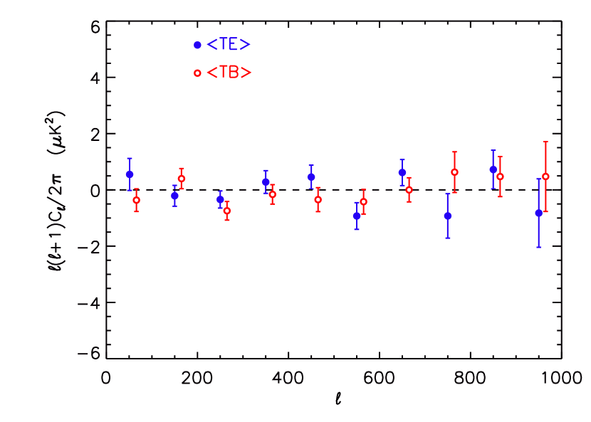
Moreover we can directly test the contamination due to dust by a correlation of our data with a dust map. If we assume that the temperature and polarization seen by Boomerang are a superposition of cmb and dust, $T_{B03}=T_{CMB}+T_{dust}$ and $E_{B03}=E_{CMB}+E_{dust}$ (and the same for $B$), then

$$\langle TE\rangle_{B03}=\langle T_{CMB}E_{CMB}\rangle+\langle T_{dust}E_{dust}\rangle$$ (9)

where we assume that dust and cmb are not correlated ($\langle T_{CMB}E_{dust}\rangle=\langle T_{dust}E_{CMB}\rangle=0$). Under the same assumption, the contaminating term $\langle T_{dust}E_{dust}\rangle$ can be estimated by

$$\langle T_{dust}E_{dust}\rangle\simeq\langle T_{dust}E_{B03}\rangle$$ (10)

We estimate $T_{dust}$ by using IRAS maps re-calibrated with DIRBE at 100 $\mu m$, extrapolated to our wavelength with model 8 in Finkbeiner et al. (1999) as described in Masi et al. (2001). We resample the extrapolated dust map with the Boomerang scan strategy, and then recreate a dust map with the same time domain filtering, flagging, and map-making algorithm as the Boomerang map. As shown in Figure 4 this contaminant is compatible with zero and two orders of magnitude lower than the detected $\langle TE\rangle$.

4. Control of systematic effects

The standard test to detect systematic effects consists of splitting the data in two subsets (jackknife), making a differenced map using the two subsets and calculating the power spectra of the differenced map divided by two to maintain the same noise statistics as an average map. The result must be consistent with zero. This test is particularly effective because the sample variance goes to zero and the noise in equation (2) reduces to

$$\sigma^{2}_{TE,b}={{2}\over{(2\ell_{b}+1)f_{\rm{sky}}\Delta\ell}}\left({{\mathcal{N}_{T,b}\mathcal{N}_{E,b}}\over{B_{b}^{4}}}\right)$$ (11)

We performed two such tests, splitting the data in time and in channels. As our temporal splitting we take the first half of the scans on the shallow region and the first half of the scans on the deep region versus the second half of shallow plus second half of deep. As our channel splitting we take two PSB pairs (W1, W2, X1, X2) versus the other two PSB pairs (Y1, Y2, Z1, Z2 for focal plane description see Masi et al., 2005). Results are reported in the bottom panels of Figures 1 and 2 and in Table 3, showing remarkable consistency with zero. This, along with the $\langle TB\rangle$=0 result presented above, gives strong evidence that the dataset is free from significant systematics.

Table 3Consistency tests

	Test	d.o.f.	$\chi^{2}$	$P_{>}$
NA	$\langle TE\rangle$ temporal	9	16.1	0.065
	$\langle TE\rangle$ channels	9	10.6	0.30
	$\langle TB\rangle$ temporal	9	13.1	0.16
	$\langle TB\rangle$ channels	9	12.3	0.20
IT	$\langle TE\rangle$ temporal	9	14.8	0.10
	$\langle TE\rangle$ channels	9	2.42	0.98
	$\langle TE\rangle$ temporal	9	7.55	0.58
	$\langle TB\rangle$ channels	9	13.5	0.14

Note. — The first bin is not used in this analysis since it can be contaminated by instrumental effects.

4.1. Propagation of instrumental uncertainties

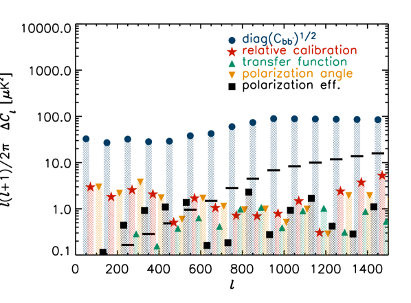
Additionally, we have modelled the potential systematic effects from mis-estimation of various instrumental characteristics using Monte Carlo simulations of signal-only time ordered data, processed varying those parameters randomly over their range of uncertainty with a Gaussian distribution. The parameters that have been changed are, the relative calibration between channels ($\pm 0.8\%$), the polarization efficiency ($\pm 0.03$), the bolometer time constants ($\pm 10\%$), the beam ($\pm 0.3^{\prime}$), and the angles of the polarizers axes respect to the telescope frame ($\pm 2^{\circ}$). These ranges are the uncertainties on those instrumental parameters as described in Masi et al. (2005).

As shown in Figure 5, the potential errors from mis-estimation of these instrumental parameters are all at least one order of magnitude lower than the statistical error-bars of the dataset. The simulation uses the $\Lambda$CDM model of Spergel et al. (2003) fit to WMAP (year 1), Acbar, and CBI.

Figure 5.— Propagation of instrumental uncertainties in the $\langle TE\rangle$ error-bars. The dots are the square root of the diagonal part of the covariance matrix, relative calibration is varied by $\pm 0.8\%$, polarization efficiency by $\pm 0.03$, time constants of the transfer function by $\pm 10\%$, the angles of the polarizers respect to the telescope frame by $\pm 2^{\circ}$, and the beam (plotted as horizontal thicks) by $\pm 0.3^{\prime}$. The error-bars ($\Delta C_{\ell}$) generated by uncertainties in instrumental characteristics are one order of magnitude lower than the errors due to noise and sampling variance (from NA pipeline here). Those error-base are not treated as an increased error, but rather as a systematic effect which is correlated bin-to-bin, and marginalized over in the parameter estimation as described in (Bridle et al., 2002).

5. Conclusion

Figure 6.— Collection of results $\langle TE\rangle$ power spectrum from recent experiments. The Boomerang data are NA and IT, with alternate binning. WMAP data are from Kogut et al. (2003), CBI from Readhead et al. (2004), DASI from Leitch et al. (2004), PIQUE from de Oliveira-Costa et al. (2003b), POLAR from de Oliveira-Costa et al. (2003a).

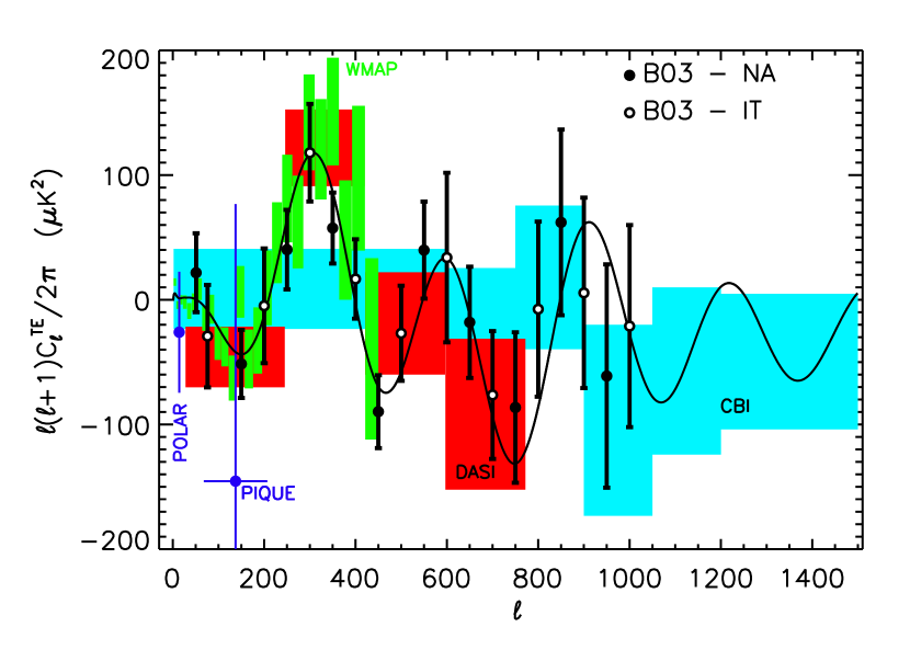
We have detected the presence of polarization of the cmb with high statistical significance (3.5 $\sigma$ combining the bins). This detection of $\langle TE\rangle$ confirms and improves previous lower frequency detections (Kogut et al., 2003; Leitch et al., 2004) using a completely independent technology. The robustness of these results against foreground contamination effects is thus strengthened, and its cosmological origin confirmed. A summary of all measurements of the $\langle TE\rangle$ spectrum is shown in Figure 6.

The B03 $\langle TE\rangle$ data show a 2 $\sigma$ anti-correlation at large angular scales ($50<\ell<150$). This, as previously detected by the WMAP experiment (Peiris et al., 2003), is consistent with the presence of superhorizon adiabatic fluctuations (Spergel & Zaldarriaga, 1997) and does not support models based on active perturbations like topological defects (Turok, 1996). In active models the perturbations are continuously produced by the causal field and lead to a positive correlation in the $\langle TE\rangle$ spectrum. While cosmic string and textures models are already ruled out by the presence of peaks in the cmb temperature power spectrum, active models may be constructed (see e.g. Durrer et al., 2001) to mimic the $\langle TT\rangle$ data but not the $\langle TE\rangle$ spectrum.

6. Acknowledgement

We gratefully acknowledge support from CIAR, CSA and NERSC in Canada, ASI, University La Sapienza and PNRA in Italy, PPARC and the Leverhulme Trust in the UK, and NASA (awards NAG5-9251 and NAG5-12723) and NSF (awards OPP-9980654 and OPP-0407592) in the USA. Additional support for detector development was provided by CIT and JPL. CBN acknowledges support from a Sloan Foundation Fellowship; WCJ and TEM were partially supported by NASA GSRP Fellowships. Field, logistical, and flight support was outstandingly supplied by USAP and NSBF; data recovery was especially appreciated. This research used resources at NERSC, supported by the DOE under Contract No. DE-AC03-76SF00098, and the MacKenzie cluster at CITA, funded by the Canada Foundation for Innovation. We also thank the CASPUR (Rome-ITALY) computational facilities and the Applied Cluster Computing Technologies Group at the Jet Propulsion Laboratory for computing time and technical support. Some of the results in this paper have been derived using the HEALPix (Górski et al., 2005) package and nearly all have benefited from the FFTW3 implementation of Fast Fourier Transform (Frigo & Johnson, 2005). The Boomerang field team is also grateful to the Coffee House at McMurdo Station, Antarctica, for existing.

References

- Baccigalupi et al. (2001) Baccigalupi, C., Burigana, C., Perrotta, F., De Zotti, G., La Porta, L., Maino, D., Maris, M., & Paladini, R. 2001, A&A, 372, 8
- Bond & Efstathiou (1984) Bond, J. R. & Efstathiou, G. 1984, ApJ, 285, L45
- Bond et al. (2000) Bond, J. R., Jaffe, A. H., & Knox, L. 2000, ApJ, 533, 19
- Bridle et al. (2002) Bridle, S. L., Crittenden, R., Melchiorri, A., Hobson, M. P., Kneissl, R., & Lasenby, A. N. 2002, MNRAS, 335, 1193
- Bucher et al. (2001) Bucher, M., Moodley, K., & Turok, N. 2001, Physical Review Letters, 87, 191301
- Coulson et al. (1994) Coulson, D., Crittenden, R. G., & Turok, N. G. 1994, Physical Review Letters, 73, 2390
- Crittenden et al. (1995) Crittenden, R. G., Coulson, D., & Turok, N. G. 1995, Phys. Rev. D, 52, 5402
- de Oliveira-Costa et al. (2003a) de Oliveira-Costa, A., Tegmark, M., O’dell, C., Keating, B., Timbie, P., Efstathiou, G., & Smoot, G. 2003a, Phys. Rev. D, 68, 083003
- de Oliveira-Costa et al. (2003b) de Oliveira-Costa, A., Tegmark, M., Zaldarriaga, M., Barkats, D., Gundersen, J. O., Hedman, M. M., Staggs, S. T., & Winstein, B. 2003b, Phys. Rev. D, 67, 023003
- Durrer et al. (2001) Durrer, R., Kunz, M., & Melchiorri, A. 2001, Phys. Rev. D, 63, 081301
- Efstathiou (1988) Efstathiou, G. 1988, Effects of reionization on microwave background anisotropies (Large-Scale Motions in the Universe: A Vatican study Week), 299–319
- Finkbeiner et al. (1999) Finkbeiner, D. P., Davis, M., & Schlegel, D. J. 1999, ApJ, 524, 867
- Frigo & Johnson (2005) Frigo, M. & Johnson, S. G. 2005, Proceedings of the IEEE, 93, 216
- Górski et al. (2005) Górski, K. M., Hivon, E., Banday, A. J., Wandelt, B. D., Hansen, F. K., Reinecke, M., & Bartelmann, M. 2005, ApJ, 622, 759
- Hivon et al. (2002) Hivon, E., Górski, K. M., Netterfield, C. B., Crill, B. P., Prunet, S., & Hansen, F. 2002, ApJ, 567, 2
- Jones et al. (2005) Jones W.C., et al. 2005, ApJ, submitted
- Kamionkowski et al. (1997) Kamionkowski, M., Kosowsky, A., & Stebbins, A. 1997, Physical Review Letters, 78, 2058
- Kogut et al. (2003) Kogut, A. et al. 2003, ApJS, 148, 161
- Kosowsky (1998) Kosowsky, A. 1998, ArXiv Astrophysics e-prints
- Kovac et al. (2002) Kovac, J. M., Leitch, E. M., Pryke, C., Carlstrom, J. E., Halverson, N. W., & Holzapfel, W. L. 2002, Nature, 420, 772
- Leitch et al. (2004) Leitch, E. M., Kovac, J. M., Halverson, N. W., Carlstrom, J. E., Pryke, C., & Smith, M. W. E. 2004, ArXiv Astrophysics e-prints
- MacTavish et al. (2005) MacTavish, C.J. et al. 2005, ApJ, submitted
- Masi et al. (2001) Masi, S. et al. 2001, ApJ, 553, L93
- Masi et al. (2005) Masi, S. et al. 2005, ApJ, submitted
- Montroy et al. (2005) Montroy, T.E. et al. 2005, ApJ, submitted
- Peiris et al. (2003) Peiris, H. V., Komatsu, E., Verde, L., Spergel, D. N., Bennett, C. L., Halpern, M., Hinshaw, G., Jarosik, N., Kogut, A., Limon, M., Meyer, S. S., Page, L., Tucker, G. S., Wollack, E., & Wright, E. L. 2003, ApJS, 148, 213
- Pogosian et al. (2002) Pogosian, L., Vachaspati, T., & Winitzki, S. 2002, Phys. Rev. D, 65, 083502
- Readhead et al. (2004) Readhead, A. C. S. et al. 2004, Science, 306, 836
- Rees (1968) Rees, M. J. 1968, ApJ, 153, L1+
- Seljak & Zaldarriaga (1996) Seljak, U. & Zaldarriaga, M. 1996, ApJ, 469, 437
- Spergel et al. (2003) Spergel, D. N. et al. 2003, ApJS, 148, 175
- Spergel & Zaldarriaga (1997) Spergel, D. N. & Zaldarriaga, M. 1997, Physical Review Letters, 79, 2180
- Tegmark et al. (2000) Tegmark, M., Eisenstein, D. J., Hu, W., & de Oliveira-Costa, A. 2000, ApJ, 530, 133
- Tucci et al. (2002) Tucci, M., Carretti, E., Cecchini, S., Nicastro, L., Fabbri, R., Gaensler, B. M., Dickey, J. M., & McClure-Griffiths, N. M. 2002, ApJ, 579, 607
- Turok (1996) Turok, N. 1996, Physical Review Letters, 77, 4138
- Zaldarriaga (1997) Zaldarriaga, M. 1997, Phys. Rev. D, 55, 1822
- Zaldarriaga & Seljak (1997) Zaldarriaga, M. & Seljak, U. 1997, Phys. Rev. D, 55, 1830