A scheme for unconventional geometric quantum computation in cavity QED

Abstract

We present a scheme for implementing the unconventional geometric two-qubit phase gate with nonzero dynamical phase by using the two-channel Raman interaction of two atoms in a cavity. We show that the dynamical phase acquired in a cyclic evolution is proportional to the geometric phase acquired in the same cyclic evolution, hence the the total phase possesses the same geometric features as the geometric phase. In our scheme the atomic excited state is adiabatically eliminated and the operation of the proposed logic gate involves only in the metastable states of the atom and hence is not affected by spontaneous emission.

I Introduction

Quantum computation employs the principle of coherent superposition and quantum entanglement to solve certain problems, such as factoring large integers and searching data in an array, much faster than a classical computer Bennett . The basic building blocks of a quantum computer are quantum logic gates. It was shown that any quantum computation can be reduced to a sequence of two classes of quantum gates, namely, universal two-qubit logic gates and one-qubit local operations Universal . The standard paradigm of quantum computation is the dynamical one where the local interactions between the qubits are controlled in such a way so that one can enact a sequence of quantum gates. On the other hand, it has been recognized that the quantum gate operations can also be implemented through the geometric effects on the wave function of the systems, this is the so-called geometric quantum computation Zanardi . Compared with the dynamical gates, the geometric quantum computation possesses practical advantages. It is well known that geometric phases depend only on some global geometric features, and do not depend on the details of the path, the time spent, the driving Hamiltonian, and the initial and final states of the evolution berryph . Therefore the geometric quantum computation is largely insensitive to local inaccuracies and fluctuations, and thus provides us a possible way to achieve fault-tolerant quantum gates.

In the implementation of geometric quantum computation, one practical question we usually meet is how to remove or avoid the dynamical phases since geometric phases are generally accompanied by dynamical ones which are not robust against local inaccuracies and fluctuations. To this end one simple method is to choose the dark states as qubit space, thus the dynamical phase is always zero duan01 . Another general method is to let the evolution be dragged by the Hamiltonian along several special closed loops, then the dynamical phases accumulated in different loops may be canceled, with the geometric phases being added ekert00 ; falci00 ; WangXB . This is the so-called multi-loop scheme.

The geometric quantum computation which is based on the cancelation of dynamical phases is referred to as conventional geometric quantum computation. Correspondingly several schemes have been presented recently to realize the so-called unconventional geometric quantum computation leibfried03 ; unzhu ; zheng ; Feng . The central idea of the unconventional geometric quantum computation is that for certain quantum evolution of a quantum system of interest one can implement fault-tolerant quantum computation by using the total phase accumulated in the evolution if it depends only on global geometric features of the evolution. In comparison with conventional geometric gates, unconventional geometric gates do not require additional operations to cancel the dynamical phases and thus simplify the realization operations. Schemes for implementing the unconventional geometric gate have been proposed in trapped ion systems leibfried03 ; unzhu and in cavity QED systemszheng ; Feng . In the schemes of cavity QED systemszheng ; Feng , the excited states are utilized as the computational bases, thus the spontaneous emission cannot be avoided in such schemes.

In this paper we make use of the two-channel Raman interaction in cavity QED two-channel ; walther to realize the unconventional geometric gate. In our scheme the atomic excited states are adiabatically eliminated and never excited during the quantum gate construction, therefore atomic spontaneous emission can be avoided in our scheme.

II Theoretical model of two-channel Raman coupling in a cavity 

We consider two identical three-level atoms in $\Lambda$-configuration placed in a high-Q cavity. The level structure of the atoms is shown  in Fig. 1, where $|e_{i}\rangle$, $|g_{i}\rangle$ ($i=1,2$) are metastable states and $|c_{i}\rangle$ is an excited state. The transitions $|c_{i}\rangle\leftrightarrow|g_{i}\rangle$ and $|c_{i}\rangle\leftrightarrow|e_{i}\rangle$ are supposed to be dipole-allowed. Each atom can be off-resonantly excited via two Raman channels by laser fields and the cavity mode. One channel is excited by two classical external fields $E_{p}(t)$ and $E_{s}(t)$ with the frequencies $\omega_{p}$ and $\omega_{s},$ respectively. The second channel contains a classical external field $E_{g}(t)$ with a frequency $\omega_{g}$ and a quantized cavity field of frequency $\omega_{c}$. Both channels are assumed to satisfy the usual Raman resonance, that is, $\omega_{p}-$ $\omega_{s}=\omega_{g}-$ $\omega_{c}=\omega_{0},$ where $\omega_{0}$ is the energy difference between levels $|e\rangle$ and $|g\rangle$. The electric field operator of the cavity mode can be expressed as $\widehat{E}_{c}=k(a+a^{\dagger})\overrightarrow{e}_{\lambda}$, where $a$ and $a^{\dagger}$ are respectively the annihilation and creation operators, $\overrightarrow{e}_{\lambda}$ is the polarization vector and $k$ is a constant determined by the quantization volume. In the case that the detunings $\delta_{1}$ and $\delta_{2}$ are sufficiently large, the atomic excited state $|c\rangle$ can be adiabatically eliminated and we can obtain an effective Hamiltonian 1. The detunings $\delta_{1}$ and $\delta_{2}$ are assumed to be sufficiently large, so that the excited state $|c\rangle$ can be eliminated.

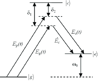
Figure 1: The two-channel Raman transition diagram. The detunings $\delta_{1}$ and $\delta_{2}$ are assumed to be sufficiently large, so that the excited state $|c\rangle$ can be eliminated.

$$H(t)=\sum_{j=1}^{2}\left[r(t)\sigma_{j}^{+}+r^{\ast}(t)\sigma_{j}^{-}\right]+\sum_{j=1}^{2}\left[g(t)a\sigma_{j}^{+}+g^{\ast}(t)a^{\dagger}\sigma_{j}^{-}\right],$$ (1)

where $\sigma^{+}=|e\rangle\langle g|$ and $\sigma^{-}=|g\rangle\langle e|$ are atomic operators, $r(t)$ and $g(t)$ are respectively the effective classical and quantum couplings and they take the following form

$$r(t) = -\frac{\left[\langle c|\overrightarrow{d}|g\rangle\cdot\overrightarrow{E}_{p}(t)\right]\left[\langle e|\overrightarrow{d}|c\rangle\cdot\overrightarrow{E}_{s}^{\ast}(t)\right]}{\delta_{1}},$$ (2)

$$g(t) = -\frac{\left[\langle c|\overrightarrow{d}|g\rangle\cdot\overrightarrow{E}_{g}(t)\right]\left[\langle e|\overrightarrow{d}|c\rangle\cdot k\overrightarrow{e}_{\lambda}\right]}{\delta_{2}}.$$ (3)

Here $\langle i|\overrightarrow{d}|j\rangle$ ($i,j=g,e,c$) denote the atomic dipole matrix elements. From above equations it is easy to note that the effective coupling parameters $r(t)$ and $g(t)$ can be controlled by adjusting the driving light fields. Based on such a feature of the Hamiltonian (1) a scheme to generate arbitrary quantum states of the cavity fields was proposed two-channel .

Now we further make the following transformation on the Hamiltonian (1)

$$H_{I}=\exp\left(iH_{0}t\right)\sum_{j=1}^{2}\left[g(t)a\sigma_{j}^{+}+g^{\ast}(t)a^{\dagger}\sigma_{j}^{-}\right]\exp\left(-iH_{0}t\right),$$ (4)

where $H_{0}=\sum_{j=1}^{2}\left[r(t)\sigma_{j}^{+}+r^{\ast}(t)\sigma_{j}^{-}\right]$. For simplicity, we assume $r(t)$ is real, then $H_{0}=r(t)\sum_{j=1}^{2}\left[\sigma_{j}^{+}+\sigma_{j}^{-}\right].$ After a simple calculation we obtain

$$H_{I} = \frac{1}{2}\sum_{j=1}^{2}\left[|+\rangle_{jj}\langle+|-|-\rangle_{jj}\langle-|+e^{i2r(t)t}|+\rangle_{jj}\langle-|\right.$$ (5)

$$\left.-e^{-i2r(t)t}|-\rangle_{jj}\langle+|\right]g(t)a+H.c.,$$

where $|\pm\rangle_{j}=(|g\rangle_{j}\pm|e\rangle_{j})/\sqrt{2}$ are eigenstates of $\sigma_{j}^{x}=\sigma_{j}^{+}+\sigma_{j}^{-}$ with eigenvalues $\pm 1$, respectively. In the strong effective classical driving regime $r(t)\gg|g|,$ the terms in Eq. (5) which oscillate with high frequencies can be eliminated in the rotating-wave approximation, and Eq. (5) can thus be simplified as

$$H_{\mathrm{eff}} = \frac{1}{2}\sum_{j=1}^{2}\left(|+\rangle_{jj}\langle+|-|-\rangle_{jj}\langle-|\right)\left[g(t)a+g^{\ast}(t)a^{\dagger}\right],$$ (6)

$$= \frac{1}{2}\left[g(t)a+g^{\ast}(t)a^{\dagger}\right]\left(\sigma_{1}^{x}+\sigma_{2}^{x}\right).$$

Similar Hamiltonians have been derived in the strongly driving Jaynes-Cummings model StrongJCM and the two-channel Raman interaction in cavity QED walther . In comparison with the trapped-ion model proposed to realize the unconventional geometric quantum computation unzhu , the Hamiltonian in our model is of a similar form to that of the trapped-ion model. In the next section we will show how to construct an unconventional geometric two-qubit phase gate based on the above Hamiltonian.

III Unconventional geometric two-qubit phase gate

We choose the eigenstates of $\sigma_{j}^{x}(j=1,2)$, that is, $|\pm\rangle_{j}=(|g\rangle_{j}\pm|e\rangle_{j})/\sqrt{2},$ as the computational basis, so that the Hamiltonian (6) will not give rise to any population changes in such a computational basis when the system is governed by the Hamiltonian (6). In the computational basis {$|+\rangle_{1}|+\rangle_{2}$, $|+\rangle_{1}|-\rangle_{2}$, $|-\rangle_{1}|+\rangle_{2}$, $|-\rangle_{1}|-\rangle_{2}$} the Hamiltonian (6) is diagonal and takes the form

$$H_{\mathrm{eff}}=\frac{1}{2}\left[g(t)a+g^{\ast}(t)a^{\dagger}\right]\times\mathrm{diag}[\lambda_{++},\lambda_{+-},\lambda_{-+},\lambda_{--}],$$ (7)

where $\lambda_{kl}$ $(k,l=+,-)$ are the eigenvales of $\left(\sigma_{1}^{x}+\sigma_{2}^{x}\right)$ and $\lambda_{++}=-\lambda_{--}=2$, $\lambda_{+-}=\lambda_{-+}=0.$ The time evolution matrix $U(t)$ is thus diagonal

$$U(t)=\mathrm{diag}\left[U_{++}(t),1,1,U_{--}(t)\right],$$ (8)

where the diagonal matrix elements $U_{kl}(t)$ can be derived from Eq. (7),

$$U_{kl}(t) = \hat{T}e^{-i\frac{1}{2}\lambda_{kl}\int_{0}^{t}\left[g(t)a+g^{\ast}(t)a^{\dagger}\right]dt},$$ (9)

$$= \lim_{N\rightarrow\infty}\prod_{n=1}^{N}e^{-i\frac{1}{2}\lambda_{kl}\left[g(t_{n})a+g^{\ast}(t_{n})a^{\dagger}\right]\Delta t},$$

$$= \lim_{N\rightarrow\infty}\prod_{n=1}^{N}D\left[\Delta\alpha_{kl}(t_{n})\right],$$

where $\hat{T}$ is the time ordering operator, $\Delta t=t/N$ is the time interval, and $\Delta\alpha_{kl}(t_{n})=-i\frac{1}{2}\lambda_{kl}g^{\ast}(t_{n})\Delta t,$ $D\left(\alpha\right)$ is the displacement operator which takes the form $D(\alpha)=\mathrm{\exp}[\alpha a^{\dagger}-\alpha^{\ast}a].$ The displacement operators satisfy the following relation

$$D(\alpha)D(\beta)=e^{i\mathrm{Im}(\alpha\beta^{\ast})}D(\alpha+\beta).$$

Based on the above formula, the Eq. (9) can be further simplified as

$$U_{kl}(t)=e^{i\gamma_{kl}}D(\int_{c}d\alpha_{kl}),$$ (10)

with $\gamma_{kl}={\rm Im}\left(\int_{c}\alpha_{kl}^{\ast}d\alpha_{kl}\right)$ and

$$d\alpha_{kl}=-i\frac{1}{2}\lambda_{kl}g^{\ast}(t)dt.$$ (11)

For a closed path $c$, $U_{kl}(t)=e^{i\gamma_{kl}}D(0)=e^{i\gamma_{kl}}.$ Here $\gamma_{kl}$ is the total phase acquired by the state $|k\rangle_{1}|l\rangle_{2}$ $(k,l=+,-)$ in the cyclic evolution from $t=0$ to $t=T$. The total phase $\gamma_{kl}$ consists of two parts, one part is geometric phase $\gamma_{kl}^{g}$, and the other part is the dynamical phase $\gamma_{kl}^{d}$ berryph . According to the coherent-state path integral methods Kuratsuji ; Hillery ; unzhu , the geometric phase $\gamma_{kl}^{g}$ and the dynamical phase $\gamma_{kl}^{d}$ can be calculated in the following way

$$\gamma_{kl}^{g} = \frac{i}{2}\int_{0}^{T}(\alpha_{kl}^{\ast}\dot{\alpha}_{kl}-\dot{\alpha}_{kl}^{\ast}\alpha_{kl})dt,$$ (12)

$$\gamma_{kl}^{d} = -\int_{0}^{T}H_{kl}(\alpha_{kl}^{\ast},\alpha_{kl};t)dt,$$ (13)

with

$$H_{kl}(\alpha_{kl}^{\ast},\alpha_{kl};t)=\langle\alpha_{kl}(t)|H_{kl}(t)|\alpha_{kl}(t)\rangle.$$ (14)

From Eq. (11) we obtain

$$\alpha_{kl}(t)=-\frac{i}{2}\lambda_{kl}\int_{0}^{t}g^{\ast}(\tau)d\tau.$$ (15)

Substituting Eq. (7) and Eq. (15) into Eq. (14), we get

$$H_{kl}(\alpha_{kl}^{\ast},\alpha_{kl};t)$$ (16)

$$= -\frac{i}{4}\lambda_{kl}^{2}\left[g(t)\int_{0}^{t}g^{\ast}(\tau)d\tau-g^{\ast}(t)\int_{0}^{t}g(\tau)d\tau\right],$$

$$= -\frac{i}{4}\lambda_{kl}^{2}G(t),$$

here for the sake of simplicity we have set $G(t)=g(t)\int_{0}^{t}g^{\ast}(\tau)d\tau-g^{\ast}(t)\int_{0}^{t}g(\tau)d\tau$. With Eq. (15) and Eq. (16), the geometric phase $\gamma_{kl}^{g}$ and the dynamical phase $\gamma_{kl}^{d}$ can be calculated according to the formulas (12) and (13),

$$\gamma_{kl}^{g} = -\frac{i}{8}\lambda_{kl}^{2}\int_{0}^{T}G(t)dt,$$ (17)

$$\gamma_{kl}^{d} = \frac{i}{4}\lambda_{kl}^{2}\int_{0}^{T}G(t)dt,$$ (18)

and the total phase is given by

$$\gamma_{kl}=\gamma_{kl}^{g}+\gamma_{kl}^{d}=\frac{i}{8}\lambda_{kl}^{2}\int_{0}^{T}G(t)dt.$$ (19)

Comparing the above three equations, we have,

$$\gamma_{kl}=\frac{1}{2}\gamma_{kl}^{d}=-\gamma_{kl}^{g}.$$ (20)

The relations between the total phase $\gamma_{kl}$, the dynamical phase $\gamma_{kl}^{d}$ and the geometric phase $\gamma_{kl}^{g}$ indicate that in the system examined here the total phase $\gamma_{kl}$ and the dynamical phase $\gamma_{kl}^{d}$ possess the global geometric features as the the geometric phase $\gamma_{kl}^{g}$ does. Therefore the cyclic evolution

$$U(T)=\mathrm{diag}\left[e^{i\gamma},1,1,e^{i\gamma}\right]$$ (21)

with $\gamma=\frac{i}{2}\int_{0}^{T}G(t)dt$ is a two-qubit phase gate operation which is robust against some lacal inaccuracies and fluctuations, this gate is nontrivial if $\gamma\neq 2n\pi.$ As described in the preceding section, the effective coupling parameter $g(t)$ can be controlled by adjusting the driving light field, so that the cyclic evolution and certain total phase $\gamma=\frac{i}{2}\int_{0}^{T}G(t)dt$ can be achieved.

It is worth noting that in our scheme the atomic excited state is adiabatically eliminated and never populated. The quantum phase gate operation only involves atomic metastable states , therefore the effect of the spontaneous emission can be ignored.

IV Conclusions

In this paper, we present a scheme for implementing the unconventional geometric two-qubit phase gate with nonzero dynamical phase by using the two-channel Raman interaction of two atoms in a cavity. We show that the dynamical phase acquired in a cyclic evolution is proportional to the geometric phase acquired in the same cyclic evolution, hence the the total phase possesses the same geometric features as the geometric phase does. In our scheme the atomic excited state is adiabatically eliminated and the operation of the proposed logic gate involves only in the metastable states of the atom and hence is not affected by spontaneous emission.

This work was supported by NUS Research Grant No. R-144-000-071-305. X.L.F. would also like to acknowledge the support of the National Natural Science Foundation of China Grant No. 60578050.

References

• (1) for a review see, e.g., C.H. Bennett, and D.P. DiVincenzo, Nature (London) 404, 247 (2000), and references therein.
• (2) D.P. DiVincenzo, Phys. Rev. A 51, 1015 (1995); S. Lloyd, Phys. Rev. Lett. 75, 346 (1995).
• (3) P. Zanardi and M. Rasetti, Phys. Lett. A 264, 94 (1999).
• (4) M. V. Berry, Proc. R. Soc. London A 392, 45 (1984); Y. Aharonov and J. Anandan, Phys. Rev. Lett. 58, 1593 (1987).
• (5) L. M. Duan, J. I. Cirac, and P. Zoller, Science 292, 1695 (2001).
• (6) J. A. Jones, V. Vedral, A. Ekert, and G. Castagnoli, Nature 403, 869 (2000).
• (7) G. Falci, R. Fazio, G. M. Palma, J. Siewert, and V. Vedral, Nature 407, 355 (2000).
• (8) X.-B. Wang and M. Keiji, Phys. Rev. Lett. 87, 097901 (2001).
• (9) D. Leibfried, B. DeMarco, V. Meyer, D. Lucas, M. Barrett, J. Britton, W. M. Itano, B. Jelenkovic,C. Langer,T. Rosenband,D. J. Wineland, Nature 422, 412 (2003).
• (10) S. L. Zhu and Z. D. Wang, Phys. Rev. Lett. 91, 187902 (2003).
• (11) S. B. Zheng, Phys. Rev. A 70, 052320 (2004).
• (12) C.-Y. Chen, M. Feng, X.-L. Zhang, K.-L. Gao, Phys. Rev. A 73, 032344 (2006).
• (13) C. K. Law and J. H. Eberly, Phys. Rev. Lett. 76, 1055 (1996) and references therein.
• (14) E. Solano, G. S. Agarwal, and H. Walther, Phys. Rev. Lett. 90, 027903 (2003).
• (15) P. Lougovski, E. Solano, and H. Walther, Phys. Rev. A 71, 013811 (2005).
• (16) H. Kuratsuji, Phys. Rev. Lett. 61, 1687 (1988).
• (17) M. Hillery and M. S. Zubairy, Phys. Rev. A 26, 451 (1982).