A study of LOCC-detection of a maximally entangled state using hypothesis testing

Abstract

We study how well answer to the question “Is the given quantum state equal to a certain maximally entangled state?” using LOCC, in the context of hypothesis testing. Under several locality and invariance conditions, optimal tests will be derived for several special cases by using basic theory of group representations. Some optimal tests are realized by performing quantum teleportation and checking whether the state is teleported. We will also give a finite process for realizing some optimal tests. The performance of the tests will be numerically compared.

J. Phys. A: Math. Gen.

1 Introduction

Entanglement plays an important role in quantum information [2, 3, 6, 21]. An experimental system makes use of a certain maximally entangled state $|\phi^{0}_{AB}\rangle$ for realization of quantum information processing. However, a state generated as a maximally entangled state is not necessarily a true maximally entangled state because the entanglement is easily corrupted by interaction with the environment. Hence, it is important to consider how well answer to the question ‘Is the state equal to $|\phi^{0}_{AB}\rangle$?’ using quantum measurement with two outcomes $(T_{0},\,T_{1})$ corresponding to (Yes, No).

For the practical use, it is natural to restrict our measurements to Local Operation and Classical Communications (LOCC) because LOCC are easily implemented. Since the result of the LOCC measurement is probabilistic and the error of incorrect answers is inevitable, it is important to consider an optimization problem of the measurement. As a framework of this argument, hypothesis testing is appropriate [13]. We consider two hypotheses

$H_{0}$: the state is $|\phi^{0}_{AB}\rangle$ versus $H_{1}$: the state is not $|\phi^{0}_{AB}\rangle$ .

Since $H_{0}$ is an accumulation point of $H_{1}$, the probability of the correct answer ‘$H_{0}$ is true’ when $H_{0}$ is really true is almost equal to the probability of the incorrect answer ‘$H_{0}$ is true’ when the state is close to $|\phi^{0}_{AB}\rangle$ but different. In the hypothesis testing, considering the two errors:
(i) To answer ‘$H_{1}$ is true’ though $H_{0}$ is really true,
(ii) To answer ‘$H_{0}$ is true’ though $H_{1}$ is really true,
we minimize the probability of (ii) with the probability of (i) kept small. See Section 2 for details.

There are similar studies based on entanglement witness; A physical observable which gives minus outputs for a set of entangled inputs [18, 24]. The concept of entanglement witness is widely adopted, and there are many extensive arguments, especially, by making use of group symmetry. See, for example, theoretical works [20, 9, 5] and experiments [1]. However, in their arguments, analysis of statistical error is not sufficient. Hence it is worth considering this problem in the style of statistical hypothesis testing [19]. Though there have been studies of quantum hypothesis testing [15, 17, 16, 25, 10, 11, 13], there have not been enough arguments for testing entanglement.

In this article, we give an approach to the hypothesis testing whether the state is $|\phi^{0}_{AB}\rangle$ using LOCC measurement between two parties and independent samples. We will derive optimal LOCC tests under some group invariance. The first case we consider is testing one sample of a pair of $d$-dimensional systems using LOCC between two parties. As a physical meaning, the optimal test is equivalent to optimal teleportation using a given state partially entangled, and the error probability is the same as the fidelity of the input and the output of the teleportation. It is also found that the test is equivalent to the extreme points of LOCC measurement described by Virmani and Plenio [27] and the entanglement witness given in [5]. Next, the result is generalized for the $n$-sample case. We derive an optimal test which is invariant by $SU(d^{n})$, and its asymptotic behavior ($n\to\infty$). In the asymptotic sense, the optimal LOCC test has the same performance as the optimal test without LOCC restriction. Next, we present the main result of this article: For $d=n=2$, the optimal test using LOCC between parties and independent samples, with $SU(2)$-invariance and some additional conditions or requirements. Since these tests are characterized by invariant measure, it contains continuous operations, However, in order to implement it, they need their construction with finite basis. Then, we show how to construct the optimal measurement with finite basis, for experimental realization. Finally, we consider an optimal test using measurement non-local between samples with $SU(2)\times SU(2)$-invariance. This test is equivalent to the entanglement swapping.

This article is organized as follows. In Section 2, a general formulation of hypothesis testing is introduced. In Section 3, we state problems treated in this article. In Section 4, we consider a problem to test entanglement based on a single sample pair, and we derive an optimal test $T^{u}$. Moreover, we consider a case where there are $n$-independent pairs of samples to test entanglement. As a direct consequence of the previous section, we derive an optimal LOCC test $T^{U}$. It is also shown that this test has the same performance as the optimal test without LOCC restriction in an asymptotic sense. In Section 5, an optimal test $T^{V}$ is derived under an LOCC condition between AB-parties and between samples. In Section 6, an optimal test $T^{W}$ is also derived under another condition which is less restrictive as for locality. In Section 7, we discretize the test derived in Section 5 using representation of a finite groups. In Section 8, we compare the performance of these tests for $n=2$.

2 Hypothesis testing

The main subject of this article is to test whether a given state is

$H_{0}$: the maximally entangled state $|\phi^{0}_{AB}\rangle$ or $H_{1}$: any other state

using LOCC. To setup the hypothesis testing formally, we first consider hypotheses $H_{0}$ and $H_{1}$ generally consisting of many elements. The hypothesis testing is an optimization problem with respect to error probability of a measurement with two outcomes corresponding to the two hypotheses. As described later, there are two error probabilities, and one of them will be minimized with the other one kept in a given small level.

Let ${{\cal H}}$ be a finite-dimensional Hilbert space which describes a physical system of interest. We denote the set of linear operators (matrices) on ${{\cal H}}$ (of density matrices on ${{\cal H}}$) by ${\cal L}({\cal H})$ and ${\cal S}({\cal H})$, respectively. In hypothesis testing, we assume two hypotheses the null hypothesis $H_{0}$ and the alternative hypothesis $H_{1}$, and choose two non-empty subsets ${{\cal S}}_{0}$ and ${{\cal S}}_{1}$ of ${{\cal S}}({{\cal H}})$ such that ${{\cal S}}_{0}\cap{{\cal S}}_{1}=\emptyset$, which correspond to our hypotheses. Suppose that the given state $\rho(\in{{\cal S}}({{\cal H}}))$ of the system is unknown and that $\rho\in{{\cal S}}_{0}$ or $\rho\in{{\cal S}}_{1}$. We test

$$H_{0}:\rho\in{{\cal S}}_{0}\mbox{ versus }H_{1}:\rho\in{{\cal S}}_{1}$$ (1)

by a measurement with two outcomes $T=(T_{0},T_{1})$: If the outcome $T_{i}$ is obtained, then we support the hypothesis $H_{i}$. However, the purpose of hypothesis testing is rejecting the null hypothesis $H_{0}$ and accepting $H_{1}$ with a given confidence level. Hence, we make decision only when the outcome $T_{1}$ is observed, and we reserve our decision when the outcome $T_{0}$ is observed. For simplicity, the test, or the measurement, $T$ is often described by $T_{0}$. In the hypothesis testing, there are two kinds of errors: Type 1 error is an event such that $H_{1}$ is accepted though $H_{0}$ is true. Type 2 error is an event such that $H_{0}$ is accepted though $H_{1}$ is true. Hence the type 1 error probability $\alpha(T,\rho)$ and the type 2 error probability $\beta(T,\rho)$ are given by

$$\alpha(T,\rho)={\rm Tr}(\rho T_{1})\ (\rho\in{{\cal S}}_{0}),\ \beta(T,\rho)={\rm Tr}(\rho T_{0})\ (\rho\in{{\cal S}}_{1}).$$

A test $T$ is said to be level-$\alpha$ when $\alpha(T,\rho)\leq\alpha$ for any $\rho\in{{\cal S}}_{0}$ because $\alpha$ expresses the confidence level of our decision. A quantity $1-\beta(T,\rho)$ is called power. In our main problem, we will consider level-zero tests only.

The main problem of hypothesis testing is to maximize the power, or equivalently, to minimize the type 2 error probability, of the test $T$ of level-$\alpha$. A test $T$ of level-$\alpha$ is said to be Most Powerful (MP) level-$\alpha$ at $\rho\in{{\cal S}}_{1}$ if $\beta(T,\rho)\leq\beta(T^{\prime},\rho)$ for any level-$\alpha$ test $T^{\prime}$. A test $T$ of level-$\alpha$ is said to be Uniformly Most Powerful (UMP) level-$\alpha$ if $T$ is MP level-$\alpha$ for any $\rho\in{{\cal S}}_{1}$. The UMP test is regarded as the best test. However, except for some examples, there is no UMP test because the uniformness is too strict.

In mathematical statistics, it is too difficult to solve problems when both ${{\cal S}}_{0}$ and ${{\cal S}}_{1}$ have plural elements, except for some special cases, for example, the classical bioequivalence problem [4]. Hence, it is natural to consider the case where

$${{\cal S}}_{0}:=\{\langle\phi^{0}_{AB}|\rho|\phi^{0}_{AB}\rangle\leq c\},\ {{\cal S}}_{1}:=\{\langle\phi^{0}_{AB}|\rho|\phi^{0}_{AB}\rangle>c\},$$

or

$${{\cal S}}_{0}:=\{\rho\neq|\phi^{0}_{AB}\rangle\langle\phi^{0}_{AB}|\},\ {{\cal S}}_{1}:=\{\rho=|\phi^{0}_{AB}\rangle\langle\phi^{0}_{AB}|\}.$$

However, it is also too difficult to treat the above case. Hence, we consider the case ${{\cal S}}_{0}:=\{|\phi^{0}_{AB}\rangle\langle\phi^{0}_{AB}|\}$ in this article.

If any $\rho\in{{\cal S}}_{0}\cup{{\cal S}}_{1}$ is invariant by an action of a group, e.g., transposition of the order of independent samples, we can without loss of generality restrict attention to tests exhibiting the same invariance, because the error probabilities are invariant. We may also require that $T_{0}$ should be invariant by a group action leaving ${{\cal S}}_{0}$ invariant to simplify the problem mathematically. In experiments of entanglement, only LOCC can be used, so it is required that the test is realized by LOCC.

There is a trade-off between requirement and power of a test; If there are two requirements $C_{1}$ and $C_{2}$ for a test and if $C_{1}$ is weaker than $C_{2}$, then the optimal test for $C_{1}$ is more powerful than that for $C_{2}$. If $C_{1}$ and $C_{2}$ are unitary-invariance conditions, arguments for $C_{2}$ tends to be mathematical easier. If they are locality conditions, arguments for $C_{2}$ tends to be more difficult. In the next section, we will introduce some different conditions.

3 Problems treated in this article

Suppose that $n$-independent samples are provided, that is, the state is given in the form

$$\rho=\sigma^{\otimes n}=\underbrace{\sigma\otimes\cdots\otimes\sigma}_{n}$$ (2)

for an unknown density $\sigma$ of a single sample. We test the following hypothesis with level zero:

$$H_{0}:\sigma=|\phi^{0}_{AB}\rangle\langle\phi^{0}_{AB}|\mbox{ versus }H_{1}:\sigma\neq|\phi^{0}_{AB}\rangle\langle\phi^{0}_{AB}|.$$ (3)

Here,

$$|\phi^{0}_{AB}\rangle=\frac{1}{\sqrt{d}}\sum_{i=0}^{d-1}|i\rangle_{A}\otimes|i\rangle_{B}$$

is a vector of a maximally entangled pair on two $d$-dimensional parties A and B spanned by $|0\rangle_{A},|1\rangle_{A},...,|d-1\rangle_{A}$ and $|0\rangle_{B},|1\rangle_{B},...,|d-1\rangle_{B}$, respectively. We refer to $\{|i\rangle_{A}\}$ and $\{|i\rangle_{B}\}$ as the standard basis.

Since the state is invariant by transposing the order of independent samples, we can without loss of generality impose that the tests for each case should be invariant by the same transposition. We additionally impose three types of basic conditions on tests, that is, level-zero, locality and unitary invariance. Among various level-$\alpha$ conditions, we adopt $\alpha=0$ because it is the most fundamental and the optimal tests have analytically simple forms. We use only AB-local tests, i.e., LOCC between A and B. In some cases, we also require that tests should be samplewise-local, i.e., LOCC between independent samples. Unitary invariance of the measurement is imposed for the symmetry of $\sigma^{\otimes n}$ or $(|\phi^{0}_{AB}\rangle\langle\phi^{0}_{AB}|)^{\otimes n}$.

First, we will make an LOCC test for a product system of two $d$-dimensional systems. Then, this will be generalized to the case of $n$-independent pairs of the $d\times d$ systems. For the $n$-sample case, a samplewise locality condition can be considered. Without the samplewise locality, we will derive optimal tests for any $d$ and $n$. With the samplewise locality, however, the problem is so difficult that we will derive optimal tests only for $d=n=2$.

We list three sets of conditions under which we will find best tests in Sections 4-6. Unless otherwise mentioned, AB-locality is always imposed.

Remark 1

One may think that it is impossible to prepare the plural samples of the given unknown state $\sigma$ when the state is easily corrupted by interaction. However, the density $\sigma$ represents the ensemble of states generated by a specific state generator. Hence, as long as each sample is generated by this generator, it can be regarded as the state $\sigma$.

3.1 U-invariance for $n$-samples

As an action of $SU(d^{n})$, U-action $U_{AB}$ is defined as

$$U_{AB}(g)=U_{A}(g)\otimes\overline{U}_{B}(g)\mbox{ for }g\in SU(d^{n})$$ (4)

where $U_{A}$ and $U_{B}$ are the natural representations of $SU(d^{n})$ on the $d^{n}$-dimensional subsystems A and B, respectively, and $\overline{X}$ is the contragradient of $X$ with respect to the standard basis, i.e., $(\overline{X})_{i,j}=X_{j,i}$. The state $|\phi^{0}_{AB}\rangle\langle\phi^{0}_{AB}|$ is U-invariant in the sense $U_{AB}(g)|\phi^{0}_{AB}\rangle\langle\phi^{0}_{AB}|U_{AB}^{\dagger}(g)=|\phi^{0}_{AB}\rangle\langle\phi^{0}_{AB}|$. A test $T=(T_{0},T_{1})$ is said to be U-invariant if $T_{0}=U_{AB}^{\dagger}(g)T_{0}U_{AB}(g)$. Under the AB-locality condition, a UMP U-invariant test $T^{U}$ will be derived. Moreover, it will be shown that, asymptotically, $T^{U}$ has the same performance as a test which is UMP without the AB-locality or the U-invariance (Section 4).

3.2 Samplewise-locality and V-invariance for two samples

Let $d=n=2$. We require samplewise-locality, that is, in this case, a test $T$ is realized by LOCC between the first and the second samples. The V-action of $SU(2)$ is defined as

$$V_{A_{1}B_{1}A_{2}B_{2}}:=U_{A_{1}}\otimes\overline{U_{B_{1}}}\otimes U_{A_{2}}\otimes\overline{U_{B_{2}}}.$$ (5)

In the same sense as the U-invariance, $(|\phi^{0}_{AB}\rangle\langle\phi^{0}_{AB}|)^{\otimes 2}$ is V-invariant. Moreover, V leaves the set ${{\cal S}}_{1}$ invariant while U and W (defined below) do not. A test is said to be V-invariant if $V_{A_{1}B_{1}A_{2}B_{2}}^{\dagger}T_{0}V_{A_{1}B_{1}A_{2}B_{2}}$ is invariant. The V-invariance is not so strict as the U-invariance that its mathematical analysis is difficult. Hence we also consider AB-invariance. This is invariance by AB-transpositions generated by

$$|i\rangle_{A_{1}}|j\rangle_{B_{1}}|k\rangle_{A_{2}}|l\rangle_{B_{2}}\mapsto(-1)^{i+j+k+l}|1-j\rangle_{A_{1}}|1-i\rangle_{B_{1}}|1-l\rangle_{A_{2}}|1-k\rangle_{B_{2}}.$$ (6)

A UMP V-invariant test $T^{V}$ will be derived under the samplewise-locality, the AB-invariance, and termwise AB-covariance defined in Definition 1. Moreover, it will be shown that in a subset of density operators, $T^{V}$ is UMP without the termwise AB-covariance (Section 5).

3.3 W-invariance for two samples

Let $d=n=2$ again. The W-action of the direct product $SU(2)\times SU(2)$ is defined as

$$W_{A_{1}B_{1}A_{2}B_{2}}(g,h):=U_{A_{1}}(g)\otimes\overline{U_{B_{1}}}(g)\otimes U_{A_{2}}(h)\otimes\overline{U_{B_{2}}}(h)$$ (7)

for $g,h\in SU(d)$. $|\phi^{0}_{AB}\rangle\langle\phi^{0}_{AB}|$ is again W-invariant, and a test $T=(T_{0},T_{1})$ is said to be W-invariant if $W_{A_{1}B_{1}A_{2}B_{2}}^{\dagger}T_{0}W_{A_{1}B_{1}A_{2}B_{2}}$ is invariant. The W-invariance is weaker than the U-invariance but is stronger than the V-invariance. In a subset of density operators, a UMP W-invariant test $T^{W}$ is obtained (Section 6).

The U-invariance is the most strict condition and the V-invariance is the weakest as the $SU(2)$ action for $d=n=2$. As for the locality conditions, the samplewise-locality in addition to the AB-locality treated in the V-invariance case is the most strict. As is shown in Section 7 with a graph, the power of $T^{W}$ is the highest, that of $T_{U}$ is the second and that of $T^{V}$ is the lowest in a neighborhood of $H_{0}$. Hence it is recommended to use $T^{W}$ rather than $T^{U}$ when one can use non-local measurement between the two independent samples. However, asymptotically, $T^{U}$ is optimal. See Section 4.3.

4 U-invariance

In this section, as the first step, we consider the case of $n=1$. As the next step, we generalize the result to arbitrary $n$.

4.1 One-sample case

Let $n=1$. Virmani and Plenio [27] have derived extreme points of AB-local measurements using Positive Partial Transpose (PPT). We will derive the same measurement $T^{u}=\{T_{0}^{u},T_{1}^{u}\}$ as a UMP U-invariant test using property of separable measurement.

Theorem 1

For $n=1$, a UMP AB-local and U-invariant test $T_{0}^{u}$ of level-zero is given as follows:

$$T_{0}^{u}=|\phi^{0}_{AB}\rangle\langle\phi^{0}_{AB}|+\frac{1}{d+1}(I-|\phi^{0}_{AB}\rangle\langle\phi^{0}_{AB}|).$$ (8)

The type 2 error probability is

$$\beta(T_{0}^{u},\rho)=\beta(T^{u},\sigma)=\frac{d\theta+1}{d+1},$$ (9)

where $\theta=\langle\phi^{0}_{AB}|\sigma|\phi^{0}_{AB}\rangle$.

The formula (9) shows that the power of the test goes to zero as the state goes to $|\phi^{0}_{AB}\rangle$. Hence, it is difficult to reject $H_{0}$ even if $H_{1}$ is true. The case when $\sigma$ is in a neighborhood of $H_{0}$ will be highlighted in (14) and (15) in the next subsection. Other optimal tests derived in the later sections have the same property.

Remark 2

The protocol for the test $T^{u}$ is implemented using the teleportation. Suppose that Alice has a state $|\psi\rangle$ in another system $A^{\prime}$. She measures her total system $A\otimes A^{\prime}$ by the Bell basis and then she lets Bob know the result. The teleportation is completed when Bob rotates the system according to the Alice’s information. The imperfectness causes some error in the teleportation, and the fidelity $|\langle\psi|\psi^{\prime}\rangle|^{2}$ of the teleported state $|\psi^{\prime}\rangle$ is evaluated by the measurement $\{|\psi\rangle\langle\psi|,I-|\psi\rangle\langle\psi|\}$, This process is equivalent to the test $T^{u}$ with $A^{\prime}$ ignored, and the fidelity is the same as $\beta(T_{0}^{u},\rho)$.

Remark 3

Virmani and Plenio [27] has proved that $T^{u}$ is an extreme point of AB-local measurements under invariance conditions. Their work is related to our problem since an optimal test is always an extreme point though the converse is not always true. In the case $n=1$, they found that there are two extreme points. As a test, however, it is obvious that the measurement other than $T^{u}$ is not optimum as a test for the hypothesis. Hence we can also conclude that $T^{u}$ is optimum based on their approach.

D’Ariano et al[5] have also considered the same measurement as $T^{u}$, as an entanglement witness. However, it is different from the hypothesis testing because the optimization of the error probability was not considered.

Proof of Theorem 8   First, we show that $T_{0}^{u}$ can be written as a classical mixture of AB-local projective measurements, i.e.,

$$T_{0}^{u}=\int_{g\in SU(d)}(U_{A}(g)\otimes\overline{U}_{B}(g))^{\dagger}\Big{(}\sum_{i=1}^{d}|i\rangle_{A}|i\rangle_{B}\langle i|_{A}\langle i|_{B}\Big{)}(U_{A}(g)\otimes\overline{U}_{B}(g))\mu(dg),$$ (10)

where $\mu(\cdot)$ is the Haar measure on $SU(d)$. (Its full measure is $1$.) From the invariance, we can easily see that the LHS has the form $a\,|\phi^{0}_{AB}\rangle\langle\phi^{0}_{AB}|+b(I-|\phi^{0}_{AB}\rangle\langle\phi^{0}_{AB}|)$. Since

$$\Tr(\hbox{LHS of }(\ref{9-6}))=d\hbox{ and }\langle\phi^{0}_{AB}|(\hbox{LHS of }(\ref{9-6}))|\phi^{0}_{AB}\rangle=1,$$ (11)

we obtain (10).

Then, the test

$$(U_{A}(g)\otimes\overline{U}_{B}(g))^{\dagger}\Big{(}\sum_{i=1}^{d}|i\rangle_{A}|i\rangle_{B}\langle i|_{A}\langle i|_{B}\Big{)}(U_{A}(g)\otimes\overline{U}_{B}(g))$$

$$= \sum_{i=1}^{d}U_{A}(g)^{\dagger}|i\rangle_{A}\overline{U}_{B}(g)^{\dagger}|i\rangle_{B}\langle i|_{A}U_{A}(g)\langle i|_{B}\overline{U}_{B}(g)$$

can be realized by the local measurements based on the bases $\{U_{A}(g)^{\dagger}|i\rangle_{A}\}_{i=1}^{d}$ and $\{\overline{U}_{B}(g)^{\dagger}|i\rangle_{B}\}_{i=1}^{d}$. Hence, the test $T^{u}$ is realized by measuring $T=\{T_{0},T_{1}\}$ by randomly choosing $g$ subject to the Haar measure.

Next, we prove its optimality. A U-invariant test $T_{0}$ is written in the following form:

$$T_{0}=a\,|\phi^{0}_{AB}\rangle\langle\phi^{0}_{AB}|+b(I-|\phi^{0}_{AB}\rangle\langle\phi^{0}_{AB}|)$$

where $0\leq a\leq 1$ and $0\leq b\leq 1$. Since $\langle\phi^{0}_{AB}|T_{0}|\phi^{0}_{AB}\rangle=a$, $T_{0}$ is level-zero if and only if $a=1$. Hence, it is sufficient to show that any LOCC level-zero U-invariant test $T$ satisfies $b\geq(d+1)^{-1}$. Further, since $a=1$, the condition $b\geq(d+1)^{-1}$ is equivalent with the condition

$$\Tr T_{0}\geq d.$$ (12)

Now, we will show (12). Since an LOCC measurement is separable, $T_{0}$ should be separable between A and B, that is,

$$T_{0}=\sum_{i}c_{i}M_{A,i}\otimes M_{B,i}$$

where $0\leq c_{i}\leq 1$ and where $M_{A,i}$ and $M_{B,i}$ are rank-one projections on $A$ and $B$, respectively. Since ${\rm Tr}(T_{0})=a+b(d^{2}-1)=1+b(d^{2}-1)=\sum_{i}c_{i}$, our problem is to minimize $\sum_{i}c_{i}$. Let $F_{i}={\rm Tr}(M_{A,i}M_{B,i}^{T})$, where $X^{T}$ is the transpose of $X$ with respect to the standard basis. Then,

$$1=\langle\phi^{0}_{AB}|T_{0}|\phi^{0}_{AB}\rangle=\sum_{i}c_{i}\langle\phi^{0}_{AB}|M_{A,i}\otimes M_{B,i}|\phi^{0}_{AB}\rangle=\frac{\sum_{i}c_{i}{\rm Tr}(M_{A,i}M_{B,i}^{T})}{d}=\frac{\sum_{i}c_{i}F_{i}}{d}.$$

Since $0\leq F_{i}\leq 1$, we have

$${\rm Tr}(T_{0})=\sum_{i}c_{i}\geq\sum_{i}c_{i}F_{i}=d.$$ (13)

$\Box$

The unconditionally UMP level-zero test $T_{0}^{g}$ is $T_{0}^{g}=|\phi^{0}_{AB}\rangle\langle\phi^{0}_{AB}|$, and its type 2 error is $\beta(T_{0}^{g},\sigma)=\theta$. The AB-locality is reflected in the difference $(1-\theta)/(d+1)$ of the type 2 errors of $T_{0}^{u}$ and $T_{0}^{g}$.

Remark 4

In order to prove the optimality, we focused on the trace of $T_{0}$. This trace method is very powerful for treating the separable POVM element detecting a given entangled state with probability one. This method was invented in this research for the first time, and was applied to other papers [26, 14].

4.2 $n$-sample case

Theorem 1 is generalized to the case of arbitrary $n$ as follows.

Theorem 2

For any $n\geq 1$, a UMP AB-local and U-invariant test of level-zero is

$$T_{0}^{U}=(|\phi^{0}_{AB}\rangle\langle\phi^{0}_{AB}|)^{\otimes n}+\frac{1}{d^{n}+1}(I-(|\phi^{0}_{AB}\rangle\langle\phi^{0}_{AB}|)^{\otimes n}).$$

The type 2 error probability is

$$\beta(T_{0}^{U},\sigma^{\otimes n})=\frac{d^{n}\theta^{n}+1}{d^{n}+1}$$

where $\theta=\langle\phi^{0}_{AB}|\sigma|\phi^{0}_{AB}\rangle$.

Proof   The proof of Theorem 1 is directly applied by replacing the space $A$ in Theorem 1 with $A_{1}\otimes\cdots\otimes A_{n}$, $B$ with $B_{1}\otimes\cdots\otimes B_{n}$, the dimension $d$ with $d^{n}$ and the group $SU(d)$ with $SU(d^{n})$. $\Box$

4.3 Asymptotic property

For comparison, let us consider other tests:

$$T_{0}^{u,n}=(T_{0}^{u})^{\otimes n}\quad\mbox{ and }\quad T_{0}^{G}=(T_{0}^{g})^{\otimes n}=(|\phi^{0}_{AB}\rangle\langle\phi^{0}_{AB}|)^{\otimes n}.$$

Note that they are both level-zero since $T_{0}^{u}$ and $T_{0}^{g}$ are level-zero. We also note that $T_{0}^{G}$ is UMP level-zero without any condition. The type 2 error probabilities are

$$\beta(T_{0}^{u,n},\sigma^{\otimes n})=\Big{(}\frac{d\theta+1}{d+1}\Big{)}^{n},\ \beta(T_{0}^{G},\sigma^{\otimes n})=\theta^{n}.$$

Hence we have

$$\beta(T_{0}^{G},\sigma^{\otimes n})<\beta(T_{0}^{U},\sigma^{\otimes n})<\beta(T_{0}^{u,n},\sigma^{\otimes n})\quad(n\geq 2).$$

On the other hand, the asymptotic behavior of $\beta(T_{0}^{U},\sigma^{\otimes n})$ is

$$\lim_{n\to\infty}\frac{\beta(T_{0}^{U},\sigma^{\otimes n})}{\theta^{n}}=1 \mbox{ if }\theta\geq 1/d,$$ (14)

$$\lim_{n\to\infty}\frac{\beta(T_{0}^{U},\sigma^{\otimes n})}{1/d^{n}}=1 \mbox{ if }\theta<1/d.$$ (15)

It means that, if $\theta=\langle\phi^{0}_{AB}|\sigma|\phi^{0}_{AB}\rangle\geq 1/d$ then $T_{0}^{U}$ and $T_{0}^{G}$ have the same asymptotic performance not only for the exponent but also for the coefficient of the type 2 error probabilities. In this sense, the restriction of AB-locality and U-invariance does not reduce the performance of the UMP level-zero test $T_{0}^{G}$.

5 Samplewise-locality, V-invariance for $n=d=2$

We consider the case $n=d=2$. First, we derive a UMP test $T^{V}$ under the conditions of samplewise-locality, V-invariance, AB-invariance, and the termwise AB-covariance (defined in Definition 1). We then prove that this test is also UMP without the termwise AB-covariance for a subset ${\cal S}^{\prime}$ of density operators.

Before defining termwise covariance, we note that, if $T_{0}$ is AB-local and samplewise-local then $T_{0}$ is AB-separable and samplewise-separable, that is,

$$T_{0}=\sum_{i}p_{i}M_{A_{1},i}\otimes M_{B_{1},i}\otimes M_{A_{2},i}\otimes M_{B_{2},i}$$

where $M_{X}$ is a rank-one projection on the system $X$.

Definition 1

The test $T_{0}$ is said to be termwise AB-covariant if

$${\rm Tr}(M_{A_{1},i}\overline{M_{B_{1},i}^{T}})=1\mbox{ and }{\rm Tr}(M_{A_{2},i}\overline{M_{B_{2},i}^{T}})=1$$

holds.

The meaning of the termwise AB-covariance will be clarified by Hayashi [12].

Define $|\phi^{1}_{AB}\rangle$, $|\phi^{2}_{AB}\rangle$ and $|\phi^{3}_{AB}\rangle$ as follows:

$$|\phi^{1}_{AB}\rangle:=\frac{\sqrt{-1}}{\sqrt{2}}\big{(}|0\rangle_{A}\otimes|1\rangle_{B}+|1\rangle_{A}\otimes|0\rangle_{B}\big{)},$$

$$|\phi^{2}_{AB}\rangle:=\frac{1}{\sqrt{2}}\big{(}-|0\rangle_{A}\otimes|1\rangle_{B}+|1\rangle_{A}\otimes|0\rangle_{B}\big{)},$$

$$|\phi^{3}_{AB}\rangle:=\frac{\sqrt{-1}}{\sqrt{2}}\big{(}|0\rangle_{A}\otimes|0\rangle_{B}-|1\rangle_{A}\otimes|1\rangle_{B}\big{)}.$$

In this section, we frequently use the matrix expression $x_{ij}=\langle\phi^{i}_{AB}|\sigma|\phi^{j}_{AB}\rangle$ for the sake of notational convenience.

Remark 5

There is a two-to-one group homomorphism of $SU(2)$ onto $SO(3)$ as the three-dimensional subrepresentation of $U_{A}\otimes\overline{U_{B}}$. It irreducibly acts on ${\rm span}\{|\phi^{1}_{AB}\rangle,|\phi^{2}_{AB}\rangle,|\phi^{3}_{AB}\rangle\}$. Now, we regard the tensor product space $({\rm span}\{|\phi^{0}_{AB}\rangle,|\phi^{1}_{AB}\rangle,|\phi^{2}_{AB}\rangle,|\phi^{3}_{AB}\rangle\})^{\otimes 2}$ as the space $M$ of $4\times 4$ matrices spanned by the basis $e^{ij}:=|\phi^{i}_{AB}\rangle_{1}|\phi^{j}_{AB}\rangle_{2}$. $SU(2)$ acts on $M$ by $V_{A_{1}B_{1}A_{2}B_{2}}$ as follows:

$$\left[\begin{array}[]{c|c}1&0\\ \hline\cr 0&S\end{array}\right]\left[\begin{array}[]{c|ccc}e^{00}&e^{01}&e^{02}&e^{03}\\ \hline\cr e^{10}&e^{11}&e^{12}&e^{13}\\ e^{20}&e^{21}&e^{22}&e^{23}\\ e^{30}&e^{31}&e^{32}&e^{33}\\ \end{array}\right]\left[\begin{array}[]{c|c}1&0\\ \hline\cr 0&S^{T}\end{array}\right]$$ (16)

for $S\in SO(3)$. Let $K_{i}^{\pm}$, $L_{i}^{\pm}$ be $i$-dimensional subspaces of $M$ defined as follows:
$K_{6}^{+}$: The space of all $3\times 3$ symmetric matrices spanned by $e^{ij}$ $(1\leq i,j\leq 3)$,
$K_{1}^{+}$: The one-dimensional subspace of $K_{6}^{+}$ spanned by the $3\times 3$ identity matrix,
$K_{3}^{+}$: The three-dimensional subspace of $K_{6}^{+}$ spanned by $e^{ij}+e^{ji}$ $(i\neq j)$,
$K_{2}^{+}$: The two-dimensional space spanned by

$$e^{11}+\omega e^{22}+\omega^{2}e^{33}\mbox{ and }e^{11}+\omega^{2}e^{22}+\omega e^{33}$$

where $\omega$ is a solution to $\omega^{2}+\omega+1=0$,
$K_{5}^{+}:=K_{6}^{+}-K_{1}^{+}=K_{3}^{+}+K_{2}^{+}$,
$K_{3}^{-}$: The space of all $3\times 3$ alternating matrices spanned by $e^{ij}$ $(1\leq i,j\leq 3)$,
$M_{10}^{+}$: The ten-dimensional space of all $4\times 4$ symmetric matrices,
$M_{6}^{-}$: The six-dimensional space of all $4\times 4$ alternating matrices,
$L_{1}^{+}$: The one-dimensional space spanned by $e^{00}=|\phi^{0}_{AB}\rangle^{\otimes 2}$,
$L_{3}^{+}:=M_{10}^{+}-K_{6}^{+}-L_{1}^{+}$,
$L_{3}^{-}:=M_{6}^{-}-K_{3}^{-}$.
The V-action $V=U_{A_{1}}\otimes\overline{U_{B_{1}}}\otimes U_{A_{2}}\otimes\overline{U_{B_{2}}}$ is equivalent to $U_{A_{1}}\otimes U_{B_{1}}\otimes U_{A_{2}}\otimes U_{B_{2}}$ as group representation. By the V-action (or, equivalently, by the SO(3) action of the form (16)), $M$ is decomposed into subspaces of irreducible representations as

$$M=K_{5}^{+}\underbrace{\oplus K_{3}^{-}\oplus L_{3}^{+}\oplus L_{3}^{-}}_{{\rm equivalent}}\underbrace{\oplus K_{1}^{+}\oplus L_{1}^{+}}_{{\rm equivalent}}.$$ (17)

See [7, 8] for details. The decompositions into the three spaces $K_{3}^{-}$ and $L_{3}^{\pm}$ and into the two spaces $K_{1}^{+}$ and $L_{1}^{+}$ in (17) are not unique because they have the equivalent representations of three-dimension and one-dimension, respectively.

The AB-transposition simultaneously maps $|\phi^{0}_{AB}\rangle_{i}$ to $-|\phi^{0}_{AB}\rangle_{i}$ for $i=1,2$, while it leaves other $|\phi^{i}_{AB}\rangle_{i}$ invariant. Hence it acts on $M$ as

$$M\ni X\mapsto\left(\begin{array}[]{cc}-1&0\\ 0&I_{3}\end{array}\right)X\left(\begin{array}[]{cc}-1&0\\ 0&I_{3}\end{array}\right)$$ (18)

where $I_{3}$ is the three-dimensional identity matrix. Hence it makes $-1$-multiplication on $L_{3}^{\pm}$ while $K_{3}^{-}$ is left invariant. Transposition of the order of the independent samples corresponds to the matrix transposition of $M$. Hence it makes $-1$-multiplication on $K_{3}^{-}$ and $L_{3}^{-}$ while $L_{3}^{+}$ is left invariant. Therefore, by the V-action with the two types of transposition, $M$ is decomposed as

$$M=K_{5}^{+}\oplus\underbrace{K_{3}^{-}\oplus L_{3}^{+}\oplus L_{3}^{-}\oplus}_{{\rm not\ equivalent}}\underbrace{K_{1}^{+}\oplus L_{1}^{+}}_{{\rm equivalent}}.$$

By the W-action, $M$ is decomposed as

$$M=L_{1}^{+}\oplus L_{3}^{\prime}\oplus L_{3}^{\prime\prime}\oplus K_{9}$$

where $L_{3}^{\prime}$ and $L_{3}^{\prime\prime}$ are the three-dimensional spaces spanned by $x_{i,0}$ and $x_{0,j}$, respectively, and $K_{9}$ is the nine-dimensional space spanned by $x_{i,j}$ $(1\leq i,j\leq 3)$. Though $L_{3}^{\prime}$ and $L_{3}^{\prime\prime}$ has the same dimension, this decomposition is unique because the first and the second element of $SU(2)\times SU(2)$ independently act on $L_{3}^{\prime}$ and $L_{3}^{\prime\prime}$. The transposition of the order of independent samples corresponds to transposing $L_{3}^{\prime}$ and $L_{3}^{\prime\prime}$. Hence W-invariant test for $\sigma^{\otimes 2}$ has the same weight on $L_{3}^{\prime}$ and $L_{3}^{\prime\prime}$.

5.1 Termwise AB-covariance

We use the symbols $K_{i}^{\pm}$ and $L_{i}^{\pm}$ not only as the spaces but also as the projection operators. Any operator $X$ invariant by the V-action, the AB-transposition, and the transposition of the order of independent samples is of the form

$$X=w_{1}K_{5}^{+}+w_{2}K_{3}^{-}+w_{3}L_{3}^{+}+w_{4}L_{3}^{-}+J$$

where $0\leq w_{i}\leq 1$ and $J$ is an operator on the two-dimensional space $J_{2}:=K_{1}^{+}\oplus L_{1}^{+}$. Each weight $w_{i}$ and the form of $N$ of the optimal test for $|\phi^{0}_{AB}\rangle$ is obtained as follows.

Theorem 3

A UMP AB-local, samplewise-local, V-invariant, AB-invariant and termwise AB-covariant test of level-zero is given as

$$T_{0}^{V}=\frac{1}{10}K_{5}^{+}+\frac{1}{3}L_{3}^{+}+(|\phi^{0}_{AB}\rangle\langle\phi^{0}_{AB}|)^{\otimes 2}+\frac{1}{6}K_{3}^{-}+\frac{1}{3}L_{3}^{-}.$$ (19)

The type 2 error of $T_{0}^{V}$ is

$$\beta(T_{0}^{V},\sigma^{\otimes 2})=v^{T}Zv-\frac{2}{15}({\rm Re}(x_{12})^{2}+{\rm Re}(x_{23})^{2}+{\rm Re}(x_{31})^{2})$$ (20)

where

$$v=\left(\begin{array}[]{c}x_{11}-1/2\\ x_{22}-1/2\\ x_{33}-1/2\end{array}\right),\ Z=\frac{1}{15}\left(\begin{array}[]{ccc}6&7&7\\ 7&6&7\\ 7&7&6\end{array}\right).$$

Proof of Theorem 3   First, the all conditions of locality and invariance are checked by calculating the weight for each projection of

$$T_{0}^{V}=\int_{g\in SU(2)}(V_{A_{1}B_{1}A_{2}B_{2}}(g))^{\dagger}(\Pi_{00}+\Pi_{01}+\Pi_{10}+\Pi_{11})(V_{A_{1}B_{1}A_{2}B_{2}}(g))\mu(dg)$$ (21)

where $\mu(\cdot)$ is the Haar measure on $SU(2)$ and where $\Pi_{ij}$ ($i,j=0,1$) is the projection on the one-dimensional subspace spanned by

$$|i\rangle_{A_{1}}\otimes|i\rangle_{B_{1}}\otimes\frac{|0\rangle_{A_{2}}+(-1)^{j}|1\rangle_{A_{2}}}{\sqrt{2}}\otimes\frac{|0\rangle_{B_{2}}+(-1)^{j}|1\rangle_{B_{2}}}{\sqrt{2}}$$ (22)

(see also Section 7.2 bellow).

Next, we show that the type 2 error of $T_{0}^{V}$ is minimized. Any test satisfying all those conditions is given in the form

$$T_{0} = \sum_{i}q_{i}\int_{g\in SU(2)}U_{A_{1}}(g)^{\dagger}|0\rangle_{A_{1}}\langle 0|_{A_{1}}U_{A_{1}}(g)\otimes U_{B_{1}}(g)^{T}|0\rangle_{B_{1}}\langle 0|_{B_{1}}\overline{U}_{B_{1}}(g)$$

$$\otimes U_{A_{2}}(g)^{T}|\psi_{F_{i}}\rangle_{A_{2}}\langle\psi_{F_{i}}|_{A_{2}}\overline{U}_{A_{2}}(g)\otimes U_{B_{2}}(g)^{T}|\psi_{F_{i}}\rangle_{B_{2}}\langle\psi_{F_{i}}|_{B_{2}}\overline{U}_{B_{2}}(g)\mu(dg)$$

where $q_{i}\geq 0$ and

$$|\psi_{F}\rangle_{X}=\frac{\sqrt{F}|0\rangle_{X}+\sqrt{1-F}|1\rangle_{X}}{\sqrt{2}}\quad(0\leq F\leq 1).$$

For the invariance conditions, $T_{0}$ can be written as

$$T_{0}=w_{1}K_{5}^{+}+w_{2}L_{3}^{+}+J+w_{3}K_{3}^{-}+w_{4}L_{3}^{-}\quad(0\leq w_{i}\leq 1).$$

To satisfy the level-zero condition, the weight of $J$ for $L_{1}^{+}$ should be one. To minimize the type 2 error, the weight of $J$ for $K_{1}^{+}$ should be zero. Hence $T_{0}$ should be

$$T_{0}=w_{1}K_{5}^{+}+w_{2}L_{3}^{+}+L_{1}^{+}+w_{3}K_{3}^{-}+w_{4}L_{3}^{-}.$$

Define

$$m(X)=\langle 0|_{A_{1}}\langle 0|_{B_{1}}\langle\psi_{F}|_{A_{2}}\langle\psi_{F}|_{B_{2}}X|0\rangle_{A_{1}}|0\rangle_{B_{1}}|\psi_{F}\rangle_{A_{2}}|\psi_{F}\rangle_{B_{2}}.$$

By direct calculation, $m(X)$ is given as follows:

$$m(K_{5}^{+})=\frac{F^{2}-F+1}{6},\ m(L_{3}^{+})=\frac{F}{2},\ m(K_{1}^{+})=\frac{(2F-1)^{2}}{12},\ m(L_{1}^{+})=\frac{1}{4},$$

$$m(K_{3}^{-})=\frac{F(1-F)}{2},\ m(L_{3}^{-})=\frac{1-F}{2}.$$

Moreover,

$${\rm Tr}(\sigma^{\otimes 2}K_{5}^{+})= \frac{1}{3}(x_{11}+x_{22}+x_{33})^{2}+\frac{1}{6}\sum_{1\leq i<j\leq 3}(x_{ii}+x_{jj})^{2}$$ (23)

$$-\frac{4}{3}\sum_{1\leq i<j\leq 3}({\rm Im}x_{ij})^{2}+\frac{1}{3}\sum_{1\leq i<j\leq 3}|x_{ij}|^{2},$$

$${\rm Tr}(\sigma^{\otimes 2}L_{3}^{+})= \sum_{i=1}^{3}\big{(}x_{00}x_{ii}+|x_{0i}|^{2}\big{)},$$ (24)

$${\rm Tr}(\sigma^{\otimes 2}K_{1}^{+})= \frac{1}{3}\sum_{1\leq i,j\leq 3}x_{ij}^{2},$$ (25)

$${\rm Tr}(\sigma^{\otimes 2}L_{1}^{+})= x_{00}^{2},$$ (26)

$${\rm Tr}(\sigma^{\otimes 2}K_{3}^{-})= \sum_{1\leq i<j\leq 3}x_{ii}x_{jj}-\sum_{1\leq i<j\leq 3}|x_{ij}|^{2},$$ (27)

$${\rm Tr}(\sigma^{\otimes 2}L_{3}^{-})= \sum_{i=1}^{3}\big{(}x_{00}x_{ii}-|x_{0i}|^{2}\big{)}.$$ (28)

Hence, the type 2 error probability is given by

$$\beta(T_{0},\sigma^{\otimes 2})=\sum_{i}q_{i}(aF_{i}^{2}+bF_{i}+c)$$ (29)

where

$$a = \frac{(x_{11}-x_{22})^{2}+(x_{22}-x_{33})^{2}+(x_{33}-x_{11})^{2}}{15}+\frac{2}{5}\big{(}{({\rm Re}x_{12})^{2}}+{({\rm Re}x_{23})^{2}}+{({\rm Re}x_{31})^{2}}\big{)},$$

$$b = -a+\frac{({\rm Im}x_{01})^{2}+({\rm Im}x_{02})^{2}+({\rm Im}x_{03})^{2}}{6},$$

$$c = -\frac{({\rm Im}x_{01})^{2}+({\rm Im}x_{02})^{2}+({\rm Im}x_{03})^{2}}{3}+\frac{({\rm Re}x_{12})^{2}+({\rm Re}x_{23})^{2}+({\rm Re}x_{31})^{2}}{15}+v_{0}^{T}Z_{0}v_{0},$$

and where

$$v_{0}=\left(\begin{array}[]{c}x_{11}-1/2\cr x_{22}-1/2\cr x_{33}-1/2\end{array}\right),\ Z_{0}=\frac{1}{30}\left(\begin{array}[]{ccc}4&3&3\cr 3&4&3\cr 3&3&4\end{array}\right).$$

We minimize (29) under necessary conditions on $\sum_{i}q_{i}$ and $\sum_{i}q_{i}F_{i}$ as follows. Since $T_{0}$ is level-zero, we have

$$\frac{1}{4}\sum_{i}q_{i}=\langle\phi^{0}_{AB}|^{\otimes 2}T_{0}|\phi^{0}_{AB}\rangle^{\otimes 2}=1.$$ (30)

We have

$$\sum_{i}q_{i}F_{i}=2.$$ (31)

Hence, the type 2 error probability (29) is minimized if $\sum_{i}q_{i}F_{i}^{2}$ is minimized under (30) and (31). From Jensen’s inequality,

$$\sum_{i}q_{i}F_{i}^{2}=4\sum_{i}\frac{q_{i}}{4}F_{i}^{2}\geq 4(\sum_{i}\frac{q_{i}}{4}F_{i})^{2}=1.$$

The equality holds if $q_{1}=\cdots=q_{4}=1$ and $F_{1}=\cdots=F_{4}=1/2$ so that the type 2 error probability is uniformly minimized if $T_{0}=T_{0}^{V}$. Hence we obtain (19) and (20). $\Box$

5.2 Optimality without termwise AB-covariance

In this subsection, we discuss the optimality of $T^{V}$ under another conditions, removing the termwise AB-locality. In this argument, we use PPT instead of separability of measurement. PPT is a class of tests which strictly includes the set of separable/LOCC tests. Hence, a test is best among LOCC if it is LOCC and is best among PPT. The set of PPT tests satisfies some linear inequalities for weights on projections $K^{\pm}_{i}$ and $L^{\pm}_{i}$. So $T^{V}$ is optimal in PPT if it uniformly minimizes error probability under the condition of the linear inequalities.

We consider parameterized subsets of states as follows.

Definition 2

Let $S(\vartheta)$ be a set of density operators $\sigma$ satisfying the following two conditions for $x_{ij}=\langle\phi^{i}_{AB}|\sigma|\phi^{j}_{AB}\rangle$:

$$\theta=x_{00}=\langle\phi^{0}_{AB}|\sigma|\phi^{0}_{AB}\rangle\geq\vartheta,$$

and

$$\frac{1}{2}\sum_{1\leq i<j\leq 3}(x_{ii}-x_{jj})^{2}+3\sum_{1\leq i<j\leq 3}|x_{ij}|^{2}\geq 4\sum_{1\leq i<j\leq 3}({\rm Im}x_{ij})^{2},$$ (32)

or equivalently,

$$3{\rm Tr}(\sigma^{\otimes 2}K_{1}^{+})\geq{\rm Tr}(\sigma^{\otimes 2}K_{3}^{-}).$$ (33)

This condition (32) is satisfied if

$$\sigma=(1-p-q-r)|\phi^{0}_{AB}\rangle\langle\phi^{0}_{AB}|+p|\phi^{1}_{AB}\rangle\langle\phi^{1}_{AB}|+q|\phi^{2}_{AB}\rangle\langle\phi^{2}_{AB}|+r|\phi^{3}_{AB}\rangle\langle\phi^{3}_{AB}|.$$

Indeed, it holds that

$$3{\rm Tr}(\sigma^{\otimes 2}K_{1}^{+})-{\rm Tr}(\sigma^{\otimes 2}K_{3}^{-})=\frac{(p-q)^{2}+(q-r)^{2}(r-p)^{2}}{2}\geq 0.$$

Theorem 4

There is $\theta_{0}<1$ such that $T_{0}^{V}$ is UMP AB-local, samplewise-local, V-invariant, weakly AB-invariant with level-zero in ${\cal S}(\theta_{0})$.

Proof   In this proof, we deal with the alternative side $T_{1}=I-T_{0}$ of the measurement because it makes the calculation simple; $T_{1}$ has the zero weight on $L_{1}^{+}$. If $T_{1}$ satisfies all the locality and invariance conditions and if it is level-zero, then $T_{1}$ is given by

$$T_{1}=w_{1}K_{5}^{+}+w_{2}L_{3}^{+}+w_{3}K_{1}^{+}+w_{4}K_{3}^{+}+w_{5}L_{3}^{-}.$$

The power of the test is given as

$${\rm Tr}(\sigma^{\otimes 2}T_{1})=w_{1}{\rm Tr}(\sigma^{\otimes 2}K_{5}^{+})+w_{2}{\rm Tr}(\sigma^{\otimes 2}L_{3}^{+})+w_{3}{\rm Tr}(\sigma^{\otimes 2}K_{1}^{+})+w_{4}{\rm Tr}(\sigma^{\otimes 2}K_{3}^{-})+w_{5}{\rm Tr}(\sigma^{\otimes 2}L_{3}^{-}).$$

Lemma 1 shows that, if $1-\theta$ is small, the power is maximized if

$$5w_{1}+3w_{2},\ w_{2},\ w_{3},\ 5w_{1}+3w_{2}+w_{3}+3w_{4}+3w_{5},\mbox{ and }w_{5}$$ (34)

are simultaneously maximized. From Lemmas 2-4 in Appendix, $w_{1},...,w_{5}$ should satisfy

$$\frac{10w_{1}+6w_{2}-w_{3}}{12}\leq 1,$$ (35)

$$\frac{w_{3}+2(w_{4}+w_{5})}{4}\leq 1,$$ (36)

$$w_{2}=w_{5},$$ (37)

$$\frac{3}{4}(w_{2}+w_{5})\leq 1.$$ (38)

Therefore,

$$\max\{5w_{1}+3w_{2}\mid(\ref{eq:v:1}),0\leq w_{i}\leq 1\}=\frac{13}{2},$$

$$\max\{w_{2}\mid(\ref{eq:v:3}),(\ref{eq:v:4}),0\leq w_{i}\leq 1\}=\frac{2}{3},$$

$$\max\{w_{3}\mid(\ref{eq:v:1}),(\ref{eq:v:2}),0\leq w_{i}\leq 1\}=1,$$

$$\max\{5w_{1}+3w_{2}+w_{3}+3w_{4}+3w_{5}\mid 0\leq w_{i}\leq 1\}=12,$$

$$\max\{w_{5}\mid(\ref{eq:v:3}),(\ref{eq:v:4}),0\leq w_{i}\leq 1\}=\frac{2}{3},$$

and we have (19) as a solution to the linear maximization problem. $\Box$

6 W-invariance for $n=d=2$

Let $d=n=2$. In this section, we test the following hypothesis with level zero:

$$H_{0}:\sigma=|\phi^{0}_{AB}\rangle\langle\phi^{0}_{AB}|\mbox{ versus }H_{1}:1/4\leq\langle\phi^{0}_{AB}|\sigma|\phi^{0}_{AB}\rangle<1.$$ (39)

In other words, we consider the case where the set of possible states is ${\cal S}^{\prime}=\{\sigma\mid\langle\phi^{0}_{AB}|\sigma|\phi^{0}_{AB}\rangle\geq 1/4\}$.

Theorem 5

A UMP AB-local, and W-invariant for (39) of level-zero is given as follows:

$$T_{0}^{W}=|\phi^{0}_{AB}\rangle\langle\phi^{0}_{AB}|^{\otimes 2}+\frac{1}{3}(I-|\phi^{0}_{AB}\rangle\langle\phi^{0}_{AB}|)^{\otimes 2}.$$ (40)

The type 2 error probability of $T_{0}^{W}$ is

$$\beta(T_{0}^{W},\sigma^{\otimes 2})=\theta^{2}+\frac{(1-\theta)^{2}}{3}.$$ (41)

Remark 6

The test $T^{W}$ is implemented, by using the entanglement swapping from $A_{1}\otimes B_{1}$ and $A_{2}\otimes B_{2}$ to $B_{1}\otimes B_{2}$; Measuring $A_{1}\otimes A_{2}$ in the Bell basis, can create entanglement in $B_{1}\otimes B_{2}$. The success rate, or the fidelity to the maximally entangled state, of the swapping is equivalent to the type 2 error probability $\beta(T_{0}^{W},\sigma^{\otimes 2})$.

Proof of Theorem 5   $T_{0}$ is W-invariant (see Remark 5). It is also AB-local because

$$T_{0}^{W}= \int_{g,h\in SU(2)}(W_{A_{1}B_{1}A_{2}B_{2}}(g,h))^{\dagger}\Big{(}|\phi^{0}_{12}\rangle_{A}|\phi^{0}_{12}\rangle_{B}\langle\phi^{0}_{12}|_{A}\langle\phi^{0}_{12}|_{B}$$

$$+|\Psi^{+}_{12}\rangle_{A}|\Psi^{+}_{12}\rangle_{B}\langle\Psi^{+}_{12}|_{A}\langle\Psi^{+}_{12}|_{B}+|\Psi^{-}_{12}\rangle_{A}|\Psi^{-}_{12}\rangle_{B}\langle\Psi^{-}_{12}|_{A}\langle\Psi^{-}_{12}|_{B}$$

$$+|\Phi^{-}_{12}\rangle_{A}|\Phi^{-}_{12}\rangle_{B}\langle\Phi^{-}_{12}|_{A}\langle\Phi^{-}_{12}|_{B}\Big{)}(W_{A_{1}B_{1}A_{2}B_{2}}(g,h))d\mu(g,h)$$

where $\mu(\cdot,\cdot)$ is the Haar measure on $SU(2)\times SU(2)$ and where

$$|\Phi^{\pm}_{12}\rangle_{X}=\frac{|0\rangle_{X_{1}}|0\rangle_{X_{2}}\pm|1\rangle_{X_{1}}|1\rangle_{X_{2}}}{\sqrt{2}},\ |\Psi^{\pm}_{12}\rangle_{X}=\frac{|0\rangle_{X_{1}}|1\rangle_{X_{2}}\pm|1\rangle_{X_{1}}|0\rangle_{X_{2}}}{\sqrt{2}}\quad(X=A,B).$$

By Remark 5. a W-invariant test $T_{0}$ is of the form

$$T_{0}=w_{1}(K_{5}^{+}+K_{3}^{-}+K_{1}^{+})+w_{2}(L_{3}^{+}+L_{3}^{-})+w_{3}|\phi^{0}_{AB}\rangle\langle\phi^{0}_{AB}|^{\otimes 2}.$$

By the level-zero condition, $w_{3}=1$. If $\sigma\in{\cal S}^{\prime}$ then

$$9^{-1}{\rm Tr}(\sigma^{\otimes 2}(K_{5}^{+}+K_{1}^{+}+K_{3}^{-}))\leq 6^{-1}{\rm Tr}(\sigma^{\otimes 2}(L_{3}^{+}+L_{3}^{-}))$$ (42)

because

$$6^{-1}{\rm Tr}(\sigma^{\otimes 2}(L_{3}^{+}+L_{3}^{-}))-9^{-1}{\rm Tr}(\sigma^{\otimes 2}(K_{5}^{+}+K_{1}^{+}+K_{3}^{-}))$$

$$= 3^{-1}\Big{(}x_{00}-\frac{x_{11}+x_{22}+x_{33}}{3}\Big{)}(x_{11}+x_{22}+x_{33}).$$

As Theorem 4, the type 2 error probability is uniformly minimized if $3w_{1}+2w_{2}$ and $w_{2}$ are simultaneously minimized (see Lemma 5). From (13), we have

$$\min\{9w_{1}+6w_{2}\mid\mbox{AB-locality}\}=3.$$

Therefore $w_{1}=1/3$ and $w_{2}=w_{4}=0$ are the solutions to the minimization problem, and the theorem is derived. $\Box$

7 Discretization of measurements

We have expressed $T^{u}$ and $T^{V}$ as probabilistic mixtures of continuously many separable operators labeled by $SU(2)$-elements. Such continuous expressions are simple and convenient in a theoretical argument. A basic method to realize a SU-invariant measurement is to operate the system as for unitary element randomly chosen with respect to the Haar measure. However, in this method, we need to prepare continuously many operations. Therefore, it is worth noting that $T^{u}$ and $T^{V}$ are also expressed as mixtures of a few operators locally realized.

7.1 Discretization of $T^{u}$

We rewrite $T$ as

$$T^{u}_{0} = \frac{2}{3}(|0_{A}0_{B}\rangle\langle 0_{A}0_{B}|+|1_{A}1_{B}\rangle\langle 1_{A}1_{B}|)$$

$$+\frac{1}{3}(|0_{A}1_{B}\rangle\langle 0_{A}1_{B}|+|1_{A}0_{B}\rangle\langle 1_{A}0_{B}|+|0_{A}1_{B}\rangle\langle 1_{A}0_{B}|+|1_{A}0_{B}\rangle\langle 0_{A}1_{B}|)$$

$$= 3^{-1}\big{(}|0_{A}0_{B}\rangle\langle 0_{A}0_{B}|+|1_{A}1_{B}\rangle\langle 1_{A}1_{B}|+|D_{A}D_{B}\rangle\langle D_{A}D_{B}|$$

$$+|X_{A}X_{B}\rangle\langle X_{A}X_{B}|+|R_{A}L_{B}\rangle\langle R_{A}L_{B}|+|L_{A}R_{B}\rangle\langle L_{A}R_{B}|\big{)}$$

where

$$|D\rangle=\frac{|0\rangle+|1\rangle}{\sqrt{2}},\ |X\rangle=\frac{|0\rangle-|1\rangle}{\sqrt{2}},\ |R\rangle=\frac{|0\rangle+\sqrt{-1}|1\rangle}{\sqrt{2}},\ |L\rangle=\frac{|0\rangle-\sqrt{-1}|1\rangle}{\sqrt{2}}.$$

This means that one can realize $T^{u}$ by the two-values POVM $T=\{T_{0},T_{1}\}$ given in the form

$$T_{0}=|x_{A}x_{B}\rangle\langle x_{A}x_{B}|+|y_{A}y_{B}\rangle\langle y_{A}y_{B}|$$

where the orthonormal pair $(x,y)$ is chosen from $\{(0,1),(D,X),(R,L)\}$ completely at random.

We also note that a finite subgroup $\mathbb{O}$ of $SU(2)$ generated by

$$\left(\begin{array}[]{cc}\sqrt{-1}&0\\ 0&-\sqrt{-1}\end{array}\right)\mbox{ and }\frac{1}{\sqrt{2}}\left(\begin{array}[]{cc}1&-1\\ 1&1\end{array}\right)$$

transitively acts on $\{|x_{A}x_{B}\rangle\mid x=0,1,D,X,R,L\}$ by $U_{AB}(\cdot)$. $\mathbb{O}$ is the octahedral group, which is the (special) symmetry group of the octahedron and the cube. Therefore, one can also realize $T^{u}$ by

$$T_{0}=|0_{A}0_{B}\rangle\langle 0_{A}0_{B}|+|1_{A}1_{B}\rangle\langle 1_{A}1_{B}|$$

after a transformation $U_{AB}(g)$ for randomly selected $g\in\mathbb{O}$.

Remark 7

D’Ariano et al[5] have proposed a discretization of an entanglement witness: the same measurement as $T^{u}$. Their discretized measurement is also equivalent to ours. However, their analysis is not enough in the sense of hypothesis testing.

7.2 Discretization of $T^{V}$

The test $T^{V}$ is also expressed as a mixture of finite measurements as follows:

$$T_{0}^{V}=\frac{1}{24}\sum_{g\in\mathbb{O}}(V_{A_{1}B_{1}A_{2}B_{2}}(h^{*}g))^{\dagger}\Big{(}\sum_{0\leq i,j\leq 1}\frac{\Pi_{ij}+\tau_{12}(\Pi_{ij})}{2}\Big{)}V_{A_{1}B_{1}A_{2}B_{2}}(h^{*}g)$$ (43)

where $h^{*}\in SU(2)$ is defined by

$$h^{*}:\cos\Big{(}\frac{\arccos\sqrt{3/5}}{4}\Big{)}|0\rangle+\sin\Big{(}\frac{\arccos\sqrt{3/5}}{4}\Big{)}|1\rangle\mapsto|0\rangle$$

and where $\tau_{12}(\cdot)$ is the transposition of $A_{1}\otimes B_{1}$ and $A_{2}\otimes B_{2}$. Therefore, one can realize $T^{V}$ as follows. First, transform by $V_{A_{1}B_{1}A_{2}B_{2}}(h^{*}g)$ where $g\in\mathbb{O}$ is chosen completely at random. Next, by probability $1/2$, replace the sample numbering, that is, apply $\tau_{12}$. Next, measure the subsystems by

$$\begin{array}[]{c|c|c|c}A_{1}&B_{1}&A_{2}&B_{2}\\ \hline\cr\{|0\rangle,|1\rangle\}&\{|0\rangle,|1\rangle\}&\{|D\rangle,|X\rangle\}&\{|D\rangle,|X\rangle\}\end{array}$$

independently. The hypothesis $H_{0}$ is accepted if $A_{1}$ and $B_{1}$ have the same measurement result and $A_{2}$ and $B_{2}$ have the same one.

One can check (43) as follows. The subspaces $K_{3}^{\pm}$, $K_{2}^{+}$, $K_{1}^{+}$, $L_{1}^{+}$ and $L_{3}^{\pm}$ are irreducible by the V-restriction $\mathbb{O}\subset SU(2)$, and, in particular, the three-dimensional actions of $\mathbb{O}$ for $K_{3}^{+}$ and $L_{3}^{+}$ are mutually inequivalent. and, by calculation,

$${\rm Tr}(K_{3}^{+}V_{A_{1}B_{1}A_{2}B_{2}}(h_{x})^{\dagger}\Pi_{ij}V_{A_{1}B_{1}A_{2}B_{2}}(h_{x})) = \frac{\cos^{2}(4x)}{8},$$ (44)

$${\rm Tr}(K_{2}^{+}V_{A_{1}B_{1}A_{2}B_{2}}(h_{x})^{\dagger}\Pi_{ij}V_{A_{1}B_{1}A_{2}B_{2}}(h_{x})) = \frac{\sin^{2}(4x)}{8}$$ (45)

where

$$SU(2)\ni h_{x}:\cos x|0\rangle+\sin x|1\rangle\mapsto|0\rangle,$$

and hence $(\ref{eq:oct:1})=(\ref{eq:oct:2})$ if $x=(\arccos\sqrt{3/5})/4$.

8 Discussion and conclusion

For $d=n=2$, we have proposed five measurements $T^{G}$, $T^{u,2}$, $T^{U}$, $T^{V}$ and $T^{W}$ as optimal tests (for subsets of states, if necessary,) in the corresponding classes of tests, that is,
${\cal T}^{G}$: the class of level-zero tests,
${\cal T}^{u,2}$: the class of level-zero tests of the form $T_{0}^{\otimes 2}$ where $T_{0}$ is AB-local U-invariant for each sample,
${\cal T}^{U}$: the class of AB-local U-invariant level-zero tests,
${\cal T}^{V}$: the class of AB-local, samplewise-local, V-invariant, weakly AB-invariant, termwise AB-covariant and level-zero tests,
${\cal T}^{W}$: the class of AB-local W-invariant tests.
The inclusion relations of these classes is not totally ordered. For example, from the locality,

$${\cal T}^{u,2},\ {\cal T}^{V}\ \subset\ {\cal T}^{U},{\cal T}^{W}\ \subset\ {\cal T}^{G}$$

while from the unitary invariance,

$${\cal T}^{U}\ \subset\ {\cal T}^{u,2},\ {\cal T}^{W}\ \subset\ {\cal T}^{V}\ \subset\ {\cal T}^{G}.$$

On the other hand, the type 2 error probabilities of the optimal tests are totally ordered:

$$\beta(\sigma^{\otimes 2},T^{G})<\beta(\sigma^{\otimes 2},T^{W})<\beta(\sigma^{\otimes 2},T^{U})<\beta(\sigma^{\otimes 2},T^{V})<\beta(\sigma^{\otimes 2},T^{u,2})$$

in a set of states close to $|\phi^{0}_{AB}\rangle$. In Figure 1, the type 2 error probabilities $\beta$ are plotted with respect to $\theta=x_{00}=\langle\phi^{0}_{AB}|\sigma|\phi^{0}_{AB}\rangle$ of $T^{u,2}$ (the highest solid line), $T^{U}$ (the second highest solid line), $T^{W}$ (the third highest solid line), $T^{G}$ (the thick line) and $T^{V}$ (the dashed line) where $x_{ij}$ are the same for $1\leq i,j\leq 3$. If $x_{ij}=0$ for $i\neq j$, then the line of $T^{V}$ coincides with that of $T^{U}$ and there is no change for other tests. In such a way, the framework of hypothesis testing clarifies the hierarchy of requirements for measurements from the viewpoint of performance of optimal tests.

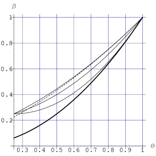
Figure 1: The type 2 error probabilities $\beta$ with respect to $\theta=x_{00}=\langle\phi^{0}_{AB}|\sigma|\phi^{0}_{AB}\rangle$ of $T^{u,2}$ (the highest solid line), $T^{U}$ (the second highest solid line), $T^{W}$ (the third highest solid line), $T^{G}$ (the thick line) and $T^{V}$ (the dashed line) where $x_{ij}$ are the same for $1\leq i,j\leq 3$.

We have considered hypothesis testing for entanglement under locality and invariance conditions. We have derived optimal tests for some settings. In our derivations of UMP tests, the separability of LOCC measurements played an important role. The UMP U-invariant and level-zero test $T^{U}$ was shown to have the asymptotically same performance as $T^{G}$. The PPT approach of Virmani and Plenio [27] was also useful to obtain UMP tests.

We may have some problems remained. One problem is how we can develop our results for general level $\alpha$ ($0<\alpha<1$), sample size $n$ and dimension $d$. Another is what test is an appropriate test for

$$H_{0}:\theta\geq c_{0}\mbox{ versus }H_{1}:\theta<c_{0},$$

$$H_{0}:\theta\leq c_{0}\mbox{ versus }H_{1}:\theta>c_{0}$$ (46)

for a constant $c_{0}$ very close to one. Indeed, if $H_{0}$ of (46) is rejected by a test with small level, then the statement ‘The state is very close to $|\phi^{0}_{AB}\rangle$’ will be strongly supported. Hence, it is siginificant to treat the hypothesis of the form (46). This problem will be treated in a forcoming paper [12]. It is also a problem remained to remove technical assumptions such as (32) in Section 5.2.

Appendix A Lemmas for Theorems 4, 5

Lemma 1

(For Theorem 4)  If $1-\theta$ is small enough, then the power of the test in Theorem 4 is uniformly maximized if (34) is simultaneously maximized.

Proof   Since $K_{i}^{\pm}$ is spanned by $x_{ij}$ and $L_{i}^{\pm}$ is spanned by $x_{i,0}$ and $x_{0,j}$ for $1\leq i,j\leq 3$, it holds that

$${\rm Tr}(\sigma^{\otimes 2}K_{i}^{+})=O\big{(}(1-\theta)^{2}\big{)}\ \mbox{ and }\ {\rm Tr}(\sigma^{\otimes 2}L_{i}^{+})=O(1-\theta)$$ (47)

as $\theta\to 1-0$, except for $L_{1}^{+}$. By (23) and (24),

$${\rm Tr}\big{(}\sigma^{\otimes 2}(3K_{5}^{+}-5K_{3}^{-})\big{)} = (x_{11}-x_{22})^{2}+(x_{22}-x_{33})^{2}+(x_{33}-x_{11})^{2}$$ (48)

$$+4({\rm Im}\,x_{12})^{2}+4({\rm Im}\,x_{23})^{2}+4({\rm Im}\,x_{31})^{2}$$

$$+6(|x_{12}|^{2}+|x_{23}|^{2}+|x_{31}|^{2})$$

$$\geq 0.$$

Define column vectors $v$ and $w$ by

$$v=\left(\begin{array}[]{ccccc}{\rm Tr}(\sigma^{\otimes 2}K_{5}^{+})&{\rm Tr}(\sigma^{\otimes 2}L_{3}^{+})&{\rm Tr}(\sigma^{\otimes 2}K_{1}^{+})&{\rm Tr}(\sigma^{\otimes 2}K_{3}^{-})&{\rm Tr}(\sigma^{\otimes 2}L_{3}^{-})\end{array}\right)^{T},$$

$$w=\left(\begin{array}[]{ccccc}w_{1}&w_{2}&w_{3}&w_{4}&w_{5}\end{array}\right)^{T},$$

and define a $5\times 5$ matrix $M$ by

$$\quad M=\frac{1}{15}\left(\begin{array}[]{ccccc}3&-9&0&0&0\cr 0&15&0&0&0\cr 0&0&15&0&0\cr-5&0&-5&5&-15\cr 0&0&0&0&15\end{array}\right)\quad\mbox{ as the inverse of }\quad\left(\begin{array}[]{ccccc}5&3&0&0&0\cr 0&1&0&0&0\cr 0&0&1&0&0\cr 5&3&1&3&3\cr 0&0&0&0&1\end{array}\right).$$

Let $v^{\prime}=M^{T}\cdot v$ and $w^{\prime}=M^{-1}\cdot w$. Each quantity in (34) is an entry of $w^{\prime}$, and the power of the test in Theorem 4 is given as $v^{T}\cdot w={v^{\prime}}^{T}\cdot w^{\prime}$. When each entry of $v^{\prime}$ is non-negative, the maximum of ${v^{\prime}}^{T}\cdot w^{\prime}$ is attained by maximizing $w^{\prime}$. From (33), (47), and (48), there is $\theta_{0}$ such that $v^{\prime}$ is non-negative. Therefore, if (34) is maximized, then the power of the test is maximized. $\Box$

Let ${\rm pt}_{C}(X)$ be the partial transpose of an operator $X$ on a subsystem $C$, for example, ${\rm pt}_{A_{1}\otimes B_{1}}(X)$ is given by

$$\quad{\rm pt}_{A_{2}B_{2}}(X)=\sum_{0\leq i,j,k,l\leq 1}I_{A_{1}B_{1}}\otimes|i\rangle_{A_{2}}|j\rangle_{B_{2}}\langle k|_{A_{2}}\langle l|_{B_{2}}XI_{A_{1}B_{1}}\otimes|i\rangle_{A_{2}}|j\rangle_{B_{2}}\langle k|_{A_{2}}\langle l|_{B_{2}}$$

where $I_{A_{2}B_{2}}$ is the identity on $A_{2}\otimes B_{2}$.

Lemma 2

(For Theorem 4)  If $T=\{T_{0},T_{1}\}$ is samplewise-local then $w_{2}=w_{5}$.

Proof   The samplewise-locality of $T$ implies that ${\rm pt}_{A_{2}\otimes B_{2}}(T_{1})$ is positive, in particular,

$$R=\left(\begin{array}[]{cc}\langle u|{\rm pt}_{A_{2}\otimes B_{2}}(T_{1})|u\rangle&\langle u|{\rm pt}_{A_{2}\otimes B_{2}}(T_{1})|v\rangle\cr\langle v|{\rm pt}_{A_{2}\otimes B_{2}}(T_{1})|u\rangle&\langle v|{\rm pt}_{A_{2}\otimes B_{2}}(T_{1})|v\rangle\end{array}\right)=\left(\begin{array}[]{cc}0&-\frac{5\sqrt{-1}}{6\sqrt{3}}(w_{2}-w_{5})\cr\frac{5\sqrt{-1}}{6\sqrt{3}}(w_{2}-w_{5})&\frac{17w_{1}+9w_{3}+w_{4}}{27}\end{array}\right)$$

should be positive where

$$|u\rangle=|\phi^{0}_{AB}\rangle_{1}|\phi^{0}_{AB}\rangle_{2},\ |v\rangle=\frac{5|\phi^{1}_{AB}\rangle_{1}|\phi^{1}_{AB}\rangle_{2}-|\phi^{2}_{AB}\rangle_{1}|\phi^{2}_{AB}\rangle_{2}-|\phi^{3}_{AB}\rangle_{1}|\phi^{3}_{AB}\rangle_{2}}{3\sqrt{3}}.$$

Since $\det(R)=-25/108(w_{2}-w_{5})^{2}\geq 0$ holds, $w_{2}=w_{5}$. $\Box$

Lemma 3

(For Theorem 4)  If $T=\{T_{0},T_{1}\}$ is AB-local then

$$0\leq\frac{10w_{1}+6w_{2}-w_{3}}{12}\leq 1,$$ (53)

$$0\leq\frac{w_{3}+2(w_{4}+w_{5})}{4}\leq 1.$$ (54)

proof  The AB-locality of $T$ implies that ${\rm pt}_{B_{1}\otimes B_{2}}(T_{0})={\rm pt}_{B_{1}\otimes B_{2}}(I-T_{1})$ is positive. The first result (53) is obtained since

$$\frac{1}{2}(\langle 0_{A_{1}}1_{B_{1}}0_{A_{2}}1_{B_{2}}|-\langle 1_{A_{1}}0_{B_{1}}1_{A_{2}}0_{B_{2}}|){\rm pt}_{B_{1}\otimes B_{2}}(T_{1})(|0_{A_{1}}1_{B_{1}}0_{A_{2}}1_{B_{2}}\rangle-|1_{A_{1}}0_{B_{1}}1_{A_{2}}0_{B_{2}}\rangle)$$

$$= \frac{10w_{1}+6w_{2}-w_{3}}{12}.$$

The second result (54) is obtained since

$$\frac{1}{2}(\langle 0_{A_{1}}0_{B_{1}}0_{A_{2}}0_{B_{2}}|-\langle 1_{A_{1}}1_{B_{1}}1_{A_{2}}1_{B_{2}}|){\rm pt}_{B_{1}\otimes B_{2}}(T_{1})(|0_{A_{1}}0_{B_{1}}0_{A_{2}}0_{B_{2}}\rangle-|1_{A_{1}}1_{B_{1}}1_{A_{2}}1_{B_{2}}\rangle)$$

$$= \frac{w_{3}+2(w_{4}+w_{5})}{4}.$$

$\Box$

Lemma 4

(For Theorem 4)  If $T=\{T_{0},T_{1}\}$ is AB-local and samplewise-local then

$$\frac{3}{4}(w_{2}+w_{5})\leq 1.$$

Proof   The AB-locality and samplewise-locality of $T$ implies that ${\rm pt}_{B_{2}}(T_{0})={\rm pt}_{B_{2}}(I-T_{1})$ is positive. Since

$$\langle\phi^{0}_{AB}|_{1}\langle\phi^{2}_{AB}|_{2}{\rm pt}_{B_{2}}(T_{1})|\phi^{0}_{AB}\rangle_{1}|\phi^{2}_{AB}\rangle_{2}=\frac{3}{4}(w_{2}+w_{5}),$$

we have the result. $\Box$

Lemma 5

(For Theorem 5)  In Theorem 5, the type 2 error probability of the test is uniformly minimized if $3w_{1}+2w_{2}$ and $w_{2}$ are simultaneously minimized.

Proof   Define column vectors $v$ and $w$ by

$$v=\left(\begin{array}[]{cc}{\rm Tr}(\sigma^{\otimes 2}(K_{5}^{+}+K_{1}^{+}+K_{3}^{-}))&{\rm Tr}(\sigma^{\otimes 2}(L_{3}^{+}+L_{3}^{-}))\end{array}\right)^{T},$$

$$w=\left(\begin{array}[]{cc}w_{1}&w_{2}\end{array}\right)^{T},$$

and define a $2\times 2$ matrix $M$ by

$$M=\frac{1}{3}\left(\begin{array}[]{cc}1&-2\cr 0&3\end{array}\right)\quad\mbox{ as the inverse of }\quad\left(\begin{array}[]{cc}3&2\cr 0&1\end{array}\right).$$

Let $v^{\prime}=M^{T}\cdot v$ and $w^{\prime}=M^{-1}\cdot w$. The power of the test in Theorem 5 is given as $v^{T}\cdot w={v^{\prime}}^{T}\cdot w^{\prime}$. If each entry of $v^{\prime}$ is non-negative, the maximum of ${v^{\prime}}^{T}\cdot w^{\prime}$ is attained by maximizing $w^{\prime}$. From (42), $v^{\prime}$ is non-negative. Therefore, if $3w_{1}+2w_{2}$ and $w_{2}$ are simultaneously minimized, the type 2 error probability is minimized. $\Box$

References

References

• [1] Barbieri, M., De Martini, F., Di Nepi, G., Mataloni, P., D’Ariano, G. M., and Macchiavello, C. 2003 Phys. Rev. Lett. 91 227901.
• [2] Bennett, C., Brassard, G., Crepeau, C., Jozsa, R., Peres, A., and Wootters, W.K. 1993 Phys. Rev. Lett. 70 1895.
• [3] Bennett, C. and Wiesner, S.J. 1992 Phys. Rev. Lett. 69 2881.
• [4] Brown, L. D., Hwang, J. T. G. and Munk, A. 1997 Ann. Statist. 25 2345-2367.
• [5] D’Ariano, G. M., Macchiavello, C. and Paris M. G. A. 2003 Phys. Rev. A 67 042310.
• [6] Ekert, A. 1991 Phys. Rev. Lett. 67 661.
• [7] Fulton, W. and Harris, J. 1991 Representation Theory; A First Course, Springer, New York.
• [8] Goodman, R. and Wallach, N. R. 1998 Representations and invariants of the classical groups, Cambridge University Press, Cambridge.
• [9] Gühne, O., Hyllus, P., Brus, D., Ekert, A., Lewenstein, M., Macchiavello, C. and Sanpera, A. 2002 Phys. Rev. A 66 062305.
• [10] Hayashi, M. 2002 J. Phys. A 35 10759-10773.
• [11] Hayashi, M. 2005 Asymptotic Theory of Quantum Statistical Inference: Selected Papers World Scientific.
• [12] Hayashi, M. in preparation.
• [13] Hayashi, M. 2006 Quantum Information: An Introduction, Springer.
• [14] Hayashi, M, Markham, D., Murao, M., Owari, M., and Virmani, S. 2006 Phys. Rev. Lett. 96 040501.
• [15] Helstrom, C. W. 1976 Quantum detection and estimation theory Academic Press.
• [16] Hiai, F. and Petz, D. 1991 Comm. Math. Phys., 143, 99-114.
• [17] Holevo, A. S. 1982 Probabilistic and statistical aspects of quantum theory, North-Holland.
• [18] Horodecki, M., Horodecki, P. and Horodecki, R. 1996 Phys. Lett. A 223 1.
• [19] Lehmann, E. L. 1986 Testing statistical hypotheses, Second edition. Wiley.
• [20] Lewenstein, M., Kraus, B., Cirac, J.I. and Horodecki, P. 2000 Phys. Rev. A 62 052310.
• [21] Nielsen, M. A. and Chuang, I. L. 2000 Quantum computation and quantum information Cambridge University Press.
• [22] Rains, E.M. 1999 Phys. Rev. A 60 173.
• [23] Rains, E.M. 2001 IEEE Trans. Inf. Theory 47 2921.
• [24] Terhal, B. M. 2000 Phys. Lett. A 271 319.
• [25] Ogawa, T. and Nagaoka, H. 2000 IEEE Trans. Inform. Theory 46 2428-2433.
• [26] Owari, M. and Hayashi, M 2005 quant-ph/0509062; to appear in Phys. Rev. A.
• [27] Virmani, S. and Plenio, M. B. 2003 Phys. Rev. A 67 062308.