Optimal Control of Coupled Josephson Qubits

Abstract

This paper is dedicated to the memory of Martti Salomaa.

Quantum optimal control theory is applied to two and three coupled Josephson charge qubits. It is shown that by using shaped pulses a cnot gate can be obtained with a trace fidelity $>0.99999$ for the two qubits, and even when including higher charge states, the leakage is below $1\%$. Yet, the required time is only a fifth of the pioneering experiment Yamamoto et al. (2003) for otherwise identical parameters. The controls have palindromic smooth time courses representable by superpositions of a few harmonics. We outline schemes to generate these shaped pulses such as simple network synthesis. The approach is easy to generalise to larger systems as shown by a fast realisation of Toffoli’s gate in three linearly coupled charge qubits. Thus it is to be anticipated that this method will find wide application in coherent quantum control of systems with finite degrees of freedom whose dynamics are Lie-algebraically closed.

In view of Hamiltonian simulation and quantum computation recent years have seen an increasing amount of quantum systems that can be coherently controlled. Next to natural microscopic quantum systems, a particular attractive candidate for scalable setups are superconducting devices based on Josephson junctions Makhlin et al. (2001). Due to the ubiquitous bath degrees of freedom in the solid-state environment, the time over which quantum coherence can be maintained remains limited, although significant progress has been achieved Bertet et al. ; Astafiev et al. (2004). Yet, it is a challenge how to produce accurate quantum gates, and how to minimize their duration such that the number of possible operations within $T_{2}$ meets the error correction threshold. Concomitantly, progress has been made in applying optimal control techniques to steer quantum systems Butkovskiy and Samoilenko (1990) in a robust, relaxation-minimising Khaneja et al. (2003) or time-optimal way Khaneja et al. (2001). Spin systems are a particularly powerful paradigm of quantum systems Glaser et al. (1998): under mild conditions they are fully controllable, i.e., local and universal quantum gates can be implemented. In $N$ spins-$\tfrac{1}{2}$ it suffices that (i) all spins can be addressed selectively by rf-pulses and (ii) that the spins form an arbitrary connected graph of weak coupling interactions. The optimal control techniques of spin systems can be extended to pseudo-spin systems, such as charge or flux states in superconducting setups, provided their Hamiltonian dynamics can be approximated to sufficient accuracy by a closed Lie algebra, e.g., in a system of $N$ qubits $\mathfrak{su}(2^{N})$.

As a practically relevant and illustrative example, we consider two capacitively coupled charge qubits controlled by DC pulses as in Ref.  Yamamoto et al. (2003). The infinite-dimensional Hilbert space of charge states in the device can be projected to its low-energy part defined by zero or one excess charge on the respective islands Makhlin et al. (2001). Identifying these charges as pseudo-spin states, the Hamiltonian can be written as $H_{\rm tot}=H_{\rm drift}+H_{\rm control}$, where the drift or static part reads (for the constants see caption to Fig. 1)

$$H_{\rm drift} = -\left(\frac{E_{m}}{4}+\frac{E_{c1}}{2}\right)(\sigma_{z}^{(1)}\otimes{\rm 1\negthickspace l}{})-\frac{E_{J1}}{2}(\sigma_{x}^{(1)}\otimes{\rm 1\negthickspace l}{})$$ (1)

$${}-\left(\frac{E_{m}}{4}+\frac{E_{c2}}{2}\right)({\rm 1\negthickspace l}{}\otimes\sigma_{z}^{(2)})-\frac{E_{J2}}{2}({\rm 1\negthickspace l}{}\otimes\sigma_{x}^{(2)})$$

$${}+\frac{E_{m}}{4}(\sigma_{z}^{(1)}\otimes\sigma_{z}^{(2)})\quad,$$

while the controls can be cast into

$$\begin{split}H_{\rm control}=&\left(\frac{E_{m}}{2}n_{g2}+{E_{c1}}n_{g1}\right)(\sigma_{z}^{(1)}\otimes{\rm 1\negthickspace l}{})\\ +&\left(\frac{E_{m}}{2}n_{g1}+{E_{c2}}n_{g2}\right)({\rm 1\negthickspace l}{}\otimes\sigma_{z}^{(2)})\quad.\end{split}$$ (2)

The control amplitudes $n_{g\nu}$, $\nu=1,2$ are gate charges controlled by external voltages via $n_{g\nu}=V_{g\nu}C_{g\nu}/2e$. They are taken to be piece-wise constant in each time interval $t_{k}$. This pseudo-spin Hamiltonian motivated by Ref. Yamamoto et al. (2003) also applies to other systems such as double quantum dots Hayashi et al. (2003) and Josephson flux qubits Majer et al. (2005), although in the latter case the controls are typically rf-pulses.

In a time interval $t_{k}$ the system thus evolves under $H_{\rm tot}^{(k)}=H_{\rm drift}+H_{\rm control}^{(k)}$. The task is to find a sequence of control amplitudes for the times $t_{1},t_{2},\dots,t_{k},\dots,t_{N}$ such as to maximise a quality function, here the overlap with the desired quantum gate or element of an algorithm $U_{\rm target}$. Moreover, for the decomposition of $U_{\rm T}=e^{-it_{N}H_{N}}e^{-it_{N-1}H_{N-1}}\cdots e^{-it_{k}H_{k}}\cdots e^{-it_{1}H_{1}}$ into available controls $\{H_{\nu}\}$ to be timeoptimal, $T:=\sum_{k=1}^{N}t_{k}$ has to be minimal. The gate fidelity is unity, if ${||U_{T}-U_{\rm target}||}_{2}=0={||U_{T}||}_{2}^{2}+{||U_{\rm target}||}_{2}^{2}-2{\rm Re\;tr}\{U_{\rm target}^{\dagger}U_{T}\}$. Maximising ${\rm Re\;tr}\{U_{\rm target}^{\dagger}U_{T}\}$ for fixed $T$ can readily be solved by optimal control: Let $h\big{(}U(t_{k})\big{)}:={\rm Re}\;{\rm tr}\{\lambda^{\dagger}(t_{k})(-i(H_{\rm d}+\sum u_{\nu}H_{\nu}))U(t_{k})\}$ with the Lagrange-type adjoint system $\lambda(t)$ following the equation of motion $\dot{\lambda}(t)=-i(H_{\rm d}+\sum u_{\nu}H_{\nu})\lambda(t)$. Pontryagin’s maximum principle requires

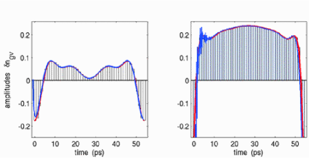
Figure 1: (Color online) Fastest charge level controls obtained for realising a cnot-gate on a pair of coupled charge qubits (left part: control qubit, right part: working qubit). The total gate charges for the qubits are $n_{g\nu}=n_{g\nu}^{(0)}+\delta n_{g\nu}$ with $\nu=1,2$. Here, $n_{g1}^{(0)}=0.24$, $n_{g2}^{(0)}=0.26$ and the qubit energies $E_{c1}/h=140.2$ GHz, $E_{c2}/h=162.2$ GHz, $E_{J1}/h=10.9$ GHz, $E_{J2}/h=9.9$ GHz, and $E_{m}/h=23.0$ GHz were chosen in accordance with the experimental values given in Yamamoto et al. (2003). The 50 piecewise constant controls are shown as bars; the trace fidelity is $\tfrac{1}{N}\big{|}{\rm tr}\{U_{\rm target}^{\dagger}U_{T}\}\big{|}>1-10^{-9}$. Red lines give the analytic curves in Eqn. 3, while the blue ones superimposed show a pulse actually synthesised by an LCR-filter (see a later section and Fig. 3).

${\partial h}/{\partial u_{\nu}}\equiv{\rm Re}\;{\rm tr}\{\lambda^{\dagger}(-iH_{\nu})U\}=0$ thus allowing to implement a gradient-flow based recursion. For the amplitude of the $\nu^{\rm th}$ control in iteration $r+1$ at time interval $t_{k}$ one finds with $\varepsilon$ as a suitably chosen step size   $n^{(r+1)}_{g\nu}(t_{k})=n^{(r)}_{g\nu}(t_{k})+\varepsilon\tfrac{\partial h^{(r)}(t_{k})}{\partial n^{(r)}_{g\nu}(t_{k})}$ as derived in Refs. Khaneja et al. (2005); Schulte-Herbrüggen et al. (2005). Here $T$ is the shortest time allowing for a given fidelity numerically.

We now turn to the discussion of our numerical results. We have used parameter values from the experiment Yamamoto et al. (2003). Variation of these values should change details of the result, but not its overall structure. Fig. 1 shows the fastest decompositions obtained by numerical optimal control for the cnot gate into evolutions under available controls (Eqns. 1 and 2). In contrast to the $250$ ps in Ref. Yamamoto et al. (2003), $T=55$ ps suffice to get ${||U_{T}-U_{\rm target}||}_{2}=5.3464\times 10^{-5}$ corresponding to a trace fidelity of $\tfrac{1}{N}\big{|}{\rm tr}\{U_{\rm target}^{\dagger}U_{T}\}\big{|}>1-10^{-9}$.

Beyond the efficient and accurate implementation, this result provides physical insight: our pulse essentially accomodates all terms of the standard cnot pulse sequence for this coupling Makhlin et al. (2001) such that different terms in the total Hamiltonian act in parallel instead of sequentially. For a cnot, the duration $T=55$ ps has to accomodate at least a $\tfrac{\pi}{2}$ rotation under the coupling Hamiltonian ($\tfrac{1}{2}\sigma_{z}\otimes\sigma_{z}$) lasting 21.7 ps concomitant to two $\tfrac{\pi}{2}$ $x$-rotations under the second of the drift components ($\tfrac{1}{2}\sigma_{x}^{(\nu)}$ with $\nu=1,2$) requiring 22.9 and 25.3 ps, respectively. Thus, unlike in NMR, the time scales of local and non-local interactions are comparable. Assume in a limiting simplification that two $\tfrac{\pi}{2}$ $x$-pulses are required, the total length cannot be shorter than $50.6$ ps. Our solution is close to this infimum. Note that a duration of $T=55$ ps also implies that the trajectory of the coherent evolution does not have to be a geodesic in the Weyl chamber (compare ref. Khaneja et al. (2001)), as shown in the supplement Fig. 5. Moreover, the evolution times for single components do not add up, indicating parallel evolution of different interactions.

The supplementary material illustrates how the sequence of controls (Fig. 1) acts in a quasi-continuous way on specific input states: Suppl. Fig. 1 gives the evolution of a product state, $|\Theta\rangle=|0\rangle|0\rangle$. The representation of the reduced states in their local Bloch spheres shows how the control qubit undergoes a closed loop, while the working qubit is inverted as expected. As demonstrated in Suppl. Fig. 2, a maximally entangled Bell state $|\psi_{+}\rangle=\tfrac{1}{\sqrt{2}}(|0\rangle|0\rangle+|1\rangle|1\rangle$ evolves from the centre of the Bloch spheres (indicating maximal entanglement) into a product state on the surface of the sphere.

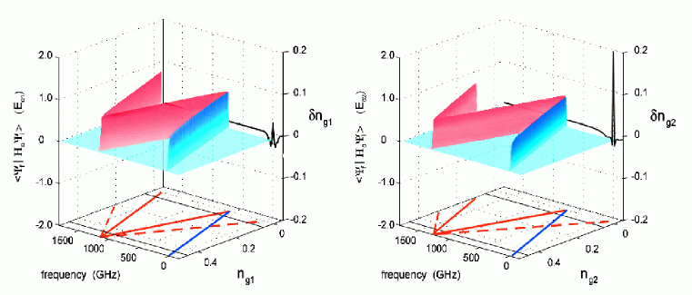
Figure 2: (Color online) Spectroscopic explanation of the high quality of the control sequences of Fig. 1: the spectral overlap of the Fourier-transforms (right walls) of the controls of Fig. 1 with the energy differences corresponding to the one-charge transitions into leakage levels (solid lines on the surface) is small at charges around $n_{g\nu}=0.2\;\text{with}\;\nu=1,2$. Intensities at allowed (solid lines) vs forbidden transitions (broken lines) into leakage levels are given in terms of the transition-matrix elements $\langle\Psi_{f}|H_{c}\Psi_{i}\rangle$ normalized by the charging energies $E_{c1}$ ($E_{c2}$) in the 3D representation: the working transitions (blue) are of the same probability as the allowed transitions into leakage levels (red) that have no overlap with the excitation bandwidth of the pulses, while the forbidden ones are too weak to show up at all. (details in the text).

Note that the time course of controls in charge qubits turns out palindromic (Fig. 1). Self-inverse gates ($U^{2}_{\rm gate}={\rm 1\negthickspace l}{}$) relate to the more general time-and-phase-reversal symmetry (TPR) observed in the control of spin systems Griesinger et al. (1987): for example, any sequence $e^{-it_{x}\sigma_{x}}e^{-it_{y}\sigma_{y}}e^{-it_{z}\sigma_{z}}$ is inverted by transposition concomitant to time reversal $t_{\nu}\mapsto-t_{\nu}$ and $\sigma_{y}\mapsto-\sigma_{y}$. Since the Hamiltonians in Eqns. 1-2 are real and symmetric, they will give the same propagator, no matter whether read forward or backward.

The pulse is not very complicated. Interestingly, the time-course of the controls on either qubit ($\nu=1,2$) can be written as a sum of $6(7)$ harmonic functions

$$n_{g\nu}(t)=\sum\limits_{j=0}^{5(6)}a_{\nu}(j)\cos\big{(}2\pi\omega_{\nu}(j)\frac{t}{T}+\phi_{\nu}(j)\big{)}\;.$$ (3)

The constants from Tab. 1 in the supplementary material give a high accuracy ($\chi^{2}=0.008231;0.003668$ for the channels 1 and 2, respectively).

This representation reflects the simplicity and the modest bandwidth of the pulses obtained. The low bandwidth allows to maintain a high fidelity even if leakage levels formed from higher charge states of the qubit system are taken into account: we now explicitly apply the full pulse to the extended Hamiltonian obtained by mapping the full Hamiltonian Yamamoto et al. (2003) to the subspaces of $-1,\dots,2$ extra charges per island. The two-qubit cnot gate is then embedded into the group $SU(16)$. Even then the propagator generated by the above controls projects well onto the cnot gate giving a trace fidelity $>0.99$. The good result may be astounding at first sight, however, it can be understood by relating the limited bandwidth to the matrix elements, which both control the transition rate: while the one-charge transitions to the leakage levels like $|-1\rangle\leftrightarrow|0\rangle$ and $|2\rangle\leftrightarrow|1\rangle$ are allowed by the Josephson coupling, the two-charge transitions like $|-1\rangle\leftrightarrow|1\rangle$ and $|2\rangle\leftrightarrow|0\rangle$ are forbidden in terms of the transition probabilities $\langle\Psi_{f}|H_{c}\Psi_{i}\rangle$ as can be seen from Fig. 2. Moreover, note that the charge levels of Fig. 1 are mostly around $n_{g}=0.2$ thus contributing to the working transition $|0\rangle\leftrightarrow|1\rangle$, while the ‘spectral overlap’ of the Fourier-transform of the time course of the controls with energy differences corresponding to the potentially deleterious one-charge transitions in Fig. 2 is small. Hence there are simple spectroscopic arguments for the high fidelity obtained by the controls of Fig. 1.

Furthermore, even the time courses starting out with any of the four canonical two-qubit basis vectors hardly ever leave the state space of the working qubits: at any time the projections onto the leakage space do not exceed $0.6\,\%$. Choosing initial states from the Bell basis entails even less leakage. Note that explicitly taking into account the leakage levels during optimisation is expected to improve the quality even further. Thus, also pseudospin systems like ours, which involve a low-energy projection disregarding leakage levels, can be controlled with high accuracy and quantum computing is not strictly limited to coupled two-level systems.

Generating these pulse shapes experimentally is a challenging but possible task. Note that the length of the pulse is given by the coupling strength as discussed above and hence can be extended by lowering the coupling.

In the pertinent time scale, there are no devices comercially available for generating arbitrary wave forms with the same capabilities as NMR-spectrometers. High-end commercial pulse generators as well as custom-built ones are close to the necessary specifications Kim et al. ; Qin et al. (2002). Pulses can be formed by superimposing short pulses of shapes easy to generate with different heights, widths, and delays. The two main candidates for this approach are (i) Gaussian pulses Hayashi et al. (2003), which can be generated at room temperature and which run nearly undistorted through the necessary cryogenic filtering and (ii) SFQ pulses, which can be generated on chip (hence avoiding the filters) using ultrafast classical Josephson electronics Brock (2001); Crankshaw et al. (2002).

We would like to exemplify a well established technique, shaping in Laplace space, to generate these pulses. The idea resembles the approach of femtosecond quantum chemistry: we start with an input current pulse $I_{\rm in}(t)$ shorter than the desired one of a shape which is arbitrary as long as it contains enough spectral weight at the harmonics necessary for the desired pulse. Such pulses are readily generated optically or electrically and have, without shaping, already been applied under cryogenic conditions Qin et al. (2002). This pulse is sent through a discrete electrical four-pole, whose transfer function $Z_{\rm 12}$ is designed such that the desired pulse is found at the output. We have carried out this idea for a rectangular pulse of length $\tau_{r}=1.1{\rm ps}$ as an input and our two gate pulses as output. We have developed a transfer function in Laplace space $Z_{12}(s)$ by fitting $V_{\rm g}(s)=Z_{12}(s)I_{\rm in}(s)$ (see Fig. 3). Owing to causality, the poles of $Z_{\rm 12}$ are either on the negative real axis or in conjugate pairs of poles on the left half plane. Each conjugate pair corresponds to an LCR-filter stage whereas each real pole corresponds to an RC lowpass-filter. It turns out, that good agreement can be achieved with 8 LCR filters and two low-pass filters, following the standard rules of circuit synthesis Rupprecht (1972).

The pulses are very close to the desired ones, see Fig. 1, and a trace fidelity of 94 % can be achieved for the entire cnot. Clearly, the quality can be further improved with more refined technology.

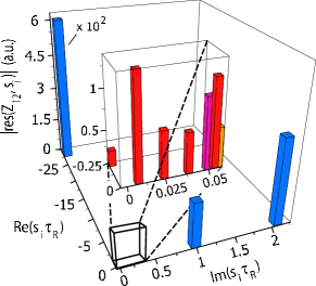
Figure 3: (Color online) Characterization of a filter shaping the pulse on the second gate. The bars show the poles $s_{i}$ of the transfer function in the Laplace plane. Poles outside the negative imaginary axis also lead to the complex conjugate pole and can be implemented by an LCR-Filter. The height of the bars show the modulus of the residue in this pole.

The filter as well as the pulse design are ready to accomodate the experimental necessities. On the one hand, due to unavoidable fabrication uncertainties, the optimum pulse will look slightly different for each individual pair of qubits. Realistically, the matrix elements of the total Hamiltonian Eqs.  (1), (2) first have to be determined spectroscopically, then our algorithm has to be run to find the optimum pulse shape. This is done on a regular PC in ca. 30 seconds. Secondly, for adjusting the filtering circuit which can be put at room temperature, one has to take into account the transfer function through the filters of the cryostat and to the sample. This contribution $Z_{\rm sample}$ to the total transfer function will most realistically be measured using a capacitor of the same geometrical dimensions of the qubits as a probe. As long as this does not block the relevant frequencies, i.e., if the setup has sufficient bandwidth, $Z_{\rm sample}$ can be accounted for when adjusting an additional pulse shaping filter such that the total transfer function shapes the correct pulse. Note, that our method also applies to control by microwave Rabi-type pulses, where pulse shaping appears to be easier as time scales are usually longer.

Likewise, in a system of three linearly coupled charge qubits, one may decompose the Toffoli gate into experimentally available controls.

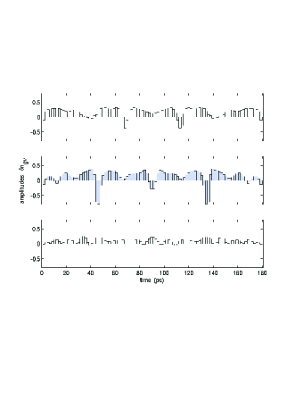
Figure 4: Fastest charge level controls obtained for realising a Toffoli-gate on a linear chain of charge qubits coupled by nearest-neighbour interactions. The piecewise constant controls are shown as bars. The trace fidelity is $\tfrac{1}{N}\big{|}{\rm tr}\{U_{\rm target}^{\dagger}U_{T}\}\big{|}>1-10^{-5}$. Here, the parameters are $E_{c1}/h=140.2$ GHz, $E_{c2}/h=120.9$ GHz, $E_{c3}/h=184.3$ GHz, $E_{J1}/h=10.9$ GHz, $E_{J2}=/h9.9$ GHz, $E_{J3}/h=9.4$ GHz,$E_{m1,m2}/h=23$ GHz, $n_{g,1}^{0}=0.24$, $n_{g,2}^{0}=0.26$, $n_{g,3}=0.28$.

This result highlights that due to the comparatively strong qubit-qubit interactions in multiqubit setups, the direct generation of three-qubit gates is much quicker than its compostion into elementary universal gates , e.g. decomposing a Toffoli into 9 cnots in a linear spin chain: the speed-up is by a factor of 2.8 compared to 9 of our cnots and by a factor of 13 compared to Nakamura’s cnots Yamamoto et al. (2003).

This also holds when developing simple algorithms Vartiainen et al. (2004) on superconducting qubit setups: a minimization algorithm for searching control amplitudes in coupled Cooper pair boxes has been applied in Niskanen et al. (2003), however, in that approach, the numerical optimization was restricted to only a few values. In Ref. Rigetti and Devoret , a pulse sequence generating a cnot with fixed couplings has been invented, which uses hard RF pulses instead of our shaped pulse and turns out to be much longer, thus leads to serious conflicts with decoherence.

In conclusion, we have constructed pulses for the realization of fast high-fidelity quantum logic gates in superconducting charge qubits. The optimum pulses are always palindromic, owing to the time-reversal invariance of these pseudo-spin Hamiltonians. The simplicity of the pulse shape results in low bandwidth and thus low leakage to higher states and the setup necessary to generate such pulses is of modest complexity.

We are indebted to Navin Khaneja for continuous stimulating scientific exchange. We thank M. Mariantoni for extensive discussions on experimental issues, specifically the transfer functions, as well as Y. Nakamura, J.M. Martinis, A. Ustinov, and D. van der Weide. This work was supported in part by Deutsche Forschungsgemeinschaft, DFG, Schwerpunkt Quanten-Informationsverarbeitung (SPP 1078: Gl 203/4-2) and SFB 631. MJS, JF, and FKW acknowledge support of ARDA and NSA through ARO contract P-43385-PH-QC.

References

- Yamamoto et al. (2003) T. Yamamoto, Y. A. Pashkin, O. Astaviev, Y. Nakamura, and J. S. Tsai, Nature (London) 425, 941 (2003).
- Makhlin et al. (2001) Y. Makhlin, G. Schön, and A. Shnirman, Rev. Mod. Phys. 73, 357 (2001).
- (3) P. Bertet, I. Chiorescu, G. Burkard, K. Semba, C. Harmans, D. DiVincenzo, and J. Mooij, cond-mat/0412485.
- Astafiev et al. (2004) O. Astafiev, Y. Pashkin, Y. Nakamura, T. Yamamoto, and J. Tsai, Phys. Rev. Lett. 93, 267007 (2004).
- Butkovskiy and Samoilenko (1990) A. G. Butkovskiy and Y. I. Samoilenko, Control of Quantum-Mechanical Processes and Systems (Kluwer, Dordrecht, 1990).
- Khaneja et al. (2003) N. Khaneja, B. Luy, and S. J. Glaser, Proc. Natl. Acad. Sci. USA 100, 13162 (2003).
- Khaneja et al. (2001) N. Khaneja, R. W. Brockett, and S. J. Glaser, Phys. Rev. A 63, 032308 (2001).
- Glaser et al. (1998) S. J. Glaser, T. Schulte-Herbrüggen, M. Sieveking, O. Schedletzky, N. C. Nielsen, O. W. Sørensen, and C. Griesinger, Science 280, 421 (1998).
- Hayashi et al. (2003) T. Hayashi, T. Fujisawa, H. Cheong, Y. Yeong, and Y. Hirayama, Phys. Rev. Lett. 91, 226804 (2003).
- Majer et al. (2005) J. Majer, F. Paauw, A. ter Haar, C. Harmans, and J. Mooij, Phys. Rev. Lett. 94, 090501 (2005).
- Khaneja et al. (2005) N. Khaneja, T. Reiss, C. Kehlet, T. Schulte-Herbrüggen, and S. J. Glaser, J. Magn. Reson. 172, 296 (2005).
- Schulte-Herbrüggen et al. (2005) T. Schulte-Herbrüggen, A. Spörl, N. Khaneja, and S. J. Glaser, e-print: quant-ph/0502104 (2005).
- Griesinger et al. (1987) C. Griesinger, C. Gemperle, O. W. Sørensen, and R. R. Ernst, Molec. Phys. 62, 295 (1987).
- (14) H. Kim, A. Kozrev, S. Ho, and D. van der Weide, proc. IEEE Microwave Symp. 2005, in press.
- Qin et al. (2002) H. Qin, R. Blick, D. van der Weide, and K. Eberl, Physica E 13, 109 (2002).
- Brock (2001) D. Brock, Int. J. High Sp. El. Sys. 11, 307 (2001).
- Crankshaw et al. (2002) D. Crankshaw, J. Habif, X. Zhou, T. Orlando, M. Feldman, and M. Bocko, IEEE Trans. Appl. Superc. 13, 966 (2002).
- Rupprecht (1972) W. Rupprecht, Netzwerksynthese (Springer, Berlin, 1972).
- Vartiainen et al. (2004) J. Vartiainen, A. Niskanen, M. Nakahara, and M. Salomaa, Int. J. Quant. Inf. 2, 1 (2004).
- Niskanen et al. (2003) A. Niskanen, J. Variainen, and M. Salomaa, Phys. Rev. Lett. 90, 197901 (2003).
- (21) C. Rigetti and M. Devoret, cond-mat/0412009.