Preparing encoded states in an oscillator

Abstract

Recently a scheme has been proposed for constructing quantum error-correcting codes that embed a finite-dimensional code space in the infinite-dimensional Hilbert space of a system described by continuous quantum variables. One of the difficult steps in this scheme is the preparation of the encoded states. We show how these states can be generated by coupling a continuous quantum variable to a single qubit. An ion trap quantum computer provides a natural setting for a continuous system coupled to a qubit. We discuss how encoded states may be generated in an ion trap.

I Introduction

It appears, in principle, that the laws of quantum mechanics allow certain mathematical problems to be solved more rapidly than can be done using a classical computer Nielsen and Chuang (2000); Preskill (1998). However, in order to accomplish this task, the state of a quantum system must maintain coherence, despite unwanted interactions with the environment. There have been a number of proposed mechanisms for protecting quantum information during a computation Shor (1995); Steane (1996); Knill and Laflamme (1996); Chau (1997); Rains (1997); Gottesman (1996); Calderbank et al. (1997). Recently, it has been shown Gottesman et al. (2001) that a $d$-dimensional quantum system (here we only consider $d=2$) can be embedded in an infinite-dimensional Hilbert space, such that a universal set of fault-tolerant quantum gates can be implemented using linear optical operations, squeezing, homodyne detection, and photon counting. The qubits are embedded in the continuous system in a manner which protects the quantum information against small shifts in the canonical quantum variables, $q$ and $p$. Ideally, the encoded states are an infinite sum of delta functions in both $q$ and $p$. Of course, such states are non-normalizable, and unphysical. Hence they must be approximated. It has been proposed Gottesman et al. (2001) that these approximate encoded states could be generated by a procedure involving a non-linear interaction Hamiltonian of the form,

$$H^{\prime} \propto qb^{\dagger}b,$$ (1)

where $q$ is the position operator of one variable, and $b$ ($b^{\dagger}$) is the annihilation (creation) operator of a second variable. Unfortunately, interactions of the form given in Eq. (1) have proven very difficult to implement. They generally require the radiation pressure of photons to move a macroscopic object (a mirror) Giovannetti et al. (2000).

Here we show that approximate encoded states can be generated by coupling the continuous variable to a single qubit, and performing a sequence of operations similar to a quantum random walk algorithm Travaglione and Milburn (2002).

In Sec. II, we briefly review the continuous variable encoding scheme proposed in Gottesman et al. Gottesman et al. (2001). In Sec. III we show how approximate encoded states can be non-deterministically generated by coupling the continuous variable to a qubit. We then discuss in Sec. IV how error recovery can be performing by deterministically preparing ancilla variables. Finally, in Sec. V we discuss how an ion trap quantum computer could be used to generate approximate encoded states, and therefore provide an important proof of principle.

II Encoding a qubit in an oscillator

Quantum computation is generally formulated in terms of interacting two level quantum systems, or qubits. The choice of two level quantum systems is partially because it is easy to draw analogies with the classical bit, but also because a two level system is the simplest non-trivial system; and increasing the number of levels only increases the computation efficiency by a constant of proportionality.

However, with the goal of building a quantum computer in mind, two level quantum systems are by no means the most natural choice. Most physical systems, even in their most elemental form, are represented by many more than two levels. Indeed, many quantum systems are naturally described by a continuous variable (infinite dimensional Hilbert space). Such continuous quantum systems have been well studied, and proposals have been made for performing analog quantum computation using such systems Braunstein (1998); Lloyd and Slotine (1998); Lloyd and Braunstein (1999).

II.1 Ideal Encoded States

Gottesman et al. Gottesman et al. (2001) discuss how to embed a qubit in a continuous quantum system, so that the extra degrees of freedom within the system can be used to correct errors which arise from unwanted interactions with the environment. Ideally, an encoded zero state, $|\bar{0}\rangle$, will be represented in position space by the wave function

$$\langle q|\bar{0}\rangle = \sum_{s=-\infty}^{\infty}\!\!\delta(q-2\alpha s)=\sum_{s=-\infty}^{\infty}\!e^{i\pi sq/\alpha},$$ (2)

and thus in momentum space, it has the wave function

$$\langle p|\bar{0}\rangle = \sum_{s=-\infty}^{\infty}\!\!\delta(p-\frac{\pi s}{\alpha})=\sum_{s=-\infty}^{\infty}\!e^{i2sp\alpha}.$$ (3)

Whilst the encoded one state, $|\bar{1}\rangle$, is represented in position and momentum space by the wave functions,

$$\langle q|\bar{1}\rangle = \sum_{s=-\infty}^{\infty}\!\!\delta(q-2\alpha(s-\frac{1}{2}))=\sum_{s=-\infty}^{\infty}\!e^{i\pi(\frac{sq}{\alpha}-1)}$$ (4)

$$\langle p|\bar{1}\rangle = \sum_{s=-\infty}^{\infty}\!\!(-1)^{s}\delta(p-\frac{\pi s}{\alpha})=\sum_{s=-\infty}^{\infty}\!e^{i(2s-1)p\alpha}.$$ (5)

The wave functions for the encoded zero state are depicted in Fig. 1(a), whilst Fig. 1(b) depicts the wave functions for the encoded one state. Clearly the zero and one encoded states are orthogonal,

$$\langle\bar{0}|\bar{1}\rangle = 0.$$ (6)

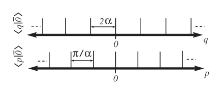
(a)
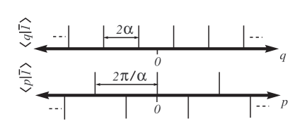
(b)

Figure 1: (a) Ideal wave function, in both position and momentum, of the encoded zero state, $|\bar{0}\rangle$. In position space, the wave-function is an infinite sum of delta functions, separated by $2\alpha$, in momentum space, the wave-function is an infinite sum of delta functions separated by $\pi/\alpha$. (b) Ideal wave functions of the encoded one state, $|\bar{1}\rangle$.

II.2 Error Recovery

For the details of how quantum computation is performed with these encoded states we direct the reader to Gottesman et al. Gottesman et al. (2001). Here we review the error recovery procedure, which protects these encoded states against shifts in position, $q$, and momentum, $p$, of size

$$|\Delta q|<\frac{\alpha}{2}\quad \mathrm{and} \quad|\Delta p|<\frac{\pi}{2\alpha}.$$ (7)

Suppose we have an encoded qubit in some arbitrary superposition of zero and one,

$$|\psi\rangle_{e} = c_{0}|\bar{0}\rangle+c_{1}|\bar{1}\rangle.$$ (8)

Assume an error occurs to the state $|\psi\rangle_{e}$, such that the wave function is shifted in the position variable by some amount $\epsilon<\alpha/2$. We wish to correct this error without destroying the state. This can be accomplished by using an ancilla variable, prepared in the state

$$|\phi\rangle_{a} = (|\bar{0}\rangle+|\bar{1}\rangle)/\sqrt{2},$$ (9)

and an interaction Hamiltonian of the form

$$H_{1} = q_{e}p_{a},$$ (10)

where the subscript $e$ denotes the encoded qubit variable, and the subscript $a$ denotes the ancilla variable. After the two systems have interacted, we can measure the $q$ variable of the ancilla system, which will allow us to determine the value of $\epsilon$. This error can then be corrected by applying an appropriate displacement operation to the encoded qubit system. Likewise, a shift of $\epsilon<\pi/2\alpha$ in the momentum variable can be corrected using an ancilla system prepared in the $|\bar{0}\rangle$ state, and evolving according to the interaction Hamiltonian,

$$H_{2} = p_{e}q_{a}.$$ (11)

III Preparing encoded states using a qubit

Once prepared, it is hoped that the error recovery procedure will be able to maintain the encoded states. However, preparation of the encoded states is not trivial. As has already been stated, we can only prepare approximate encoded states. In this section we show how approximate encoded states can be prepared with the aid of a single ancilla qubit. Our preparation scheme is non-deterministic, in that a valid approximate encoded state will only be prepared with some probability less than one, however, we will know when our preparation procedure has worked.

We shall denote approximate encoded zero and one states with the symbols $|\widetilde{0}\rangle$ and $|\widetilde{1}\rangle$. As in Gottesman et al. (2001), we begin the preparation procedure with the quantum system in the ground state of the oscillator, $|0\rangle$, and apply squeezing in the $q$ quadrature. This creates the state

$$\langle q|s\rangle = g(q,\Delta),$$ (12)

where

$$g(q,\Delta) = \frac{e^{-q^{2}/2\Delta^{2}}}{\sqrt{\Delta\sqrt{\pi}}},$$ (13)

and $\Delta$ is the width of the Gaussian and a measure of the degree of squeezing. $\Delta=1$ corresponds to the oscillator ground state, and $\Delta<1$ indicates a squeezed state. Using an ancilla qubit, initially in the zero state, $|0\rangle$, the approximate encoded one state, $|\widetilde{1}_{1}\rangle$ is then created by applying the sequence of operators,

$$\hat{H}e^{-i\alpha p_{e}\sigma_{z}}\hat{H},$$ (14)

where $\sigma_{z}$ is the Pauli $z$ matrix,

$$\sigma_{z} = \left(\begin{array}[]{cc}1&0\\ 0&-1\end{array}\right),$$ (17)

applied to the qubit, and $\hat{H}$ is the Hadamard gate,

$$\hat{H} = \frac{1}{\sqrt{2}}\left(\begin{array}[]{cc}1&1\\ 1&-1\end{array}\right),$$ (20)

applied to the qubit. Measuring the qubit in the zero state, which will occur with probability 1/2, results in the continuous variable being left in the state,

$$\langle q|\widetilde{1}_{1}\rangle = \frac{N}{\sqrt{2}}\left(g(q-\alpha,\Delta)+g(q+\alpha,\Delta)\right),$$ (21)

where $N$ is a normalization factor, which is approximately equal to one, if $\Delta/\alpha$ is small compared to one. If the qubit is measured in the one state, the encoded variable is discarded and we try again. To create improved approximate encoded states, we iterate the following procedure:
Given $|\widetilde{1}_{n-1}\rangle$, and a qubit in the state $|0\rangle$.

• Apply the operators:

  $$\hat{H}e^{-i2^{n-1}\alpha p_{e}\sigma_{z}}\hat{H}$$ (22)

• Measure the qubit.

• If the qubit is found in the state $|0\rangle$, then we have created $|\widetilde{1}_{n}\rangle$.

• Else discard and start again.

Thus, with probability $1/2^{n}$, we create the approximate encoded state

$$\langle q|\widetilde{1}_{n}\rangle = \frac{N}{\sqrt{2^{n}}}\sum_{s=1}^{2^{n}}g(q+\alpha(1\!+\!2^{n}\!-\!2s),\Delta).$$ (23)

In momentum space the approximate encoded state has wave function

$$\langle p|\widetilde{1}_{n}\rangle = \left(\frac{\Delta}{2^{n}\sqrt{\pi}}\right)^{1/2}Ne^{-(p\Delta)^{2}/2}\frac{\sin{\alpha 2^{n}p}}{\sin{\alpha p}}.$$ (24)

Fig. 2 depicts the approximate encoded state $|\widetilde{1}_{3}\rangle$, with $\Delta=0.15$ and $\alpha=\sqrt{\pi/2}$. This state will be generated with probability 1/8.

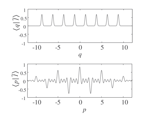
Figure 2: Wave-function, in both position and momentum, of the approximate encoded zero state, $|\widetilde{1}_{3}\rangle$. This approximate encoded state will be generated with probability 1/8, by first squeezing the continuous variable in momentum quadrature, and then applying the sequence of operations and measurements described in the text.

The approximate encoded zero state $|\widetilde{0}_{n}\rangle$ is created by displacing the state $|\widetilde{1}_{n}\rangle$ by an amount $\alpha$ in the position variable. Thus

$$\langle q|\widetilde{0}_{n}\rangle = \sum_{s=1}^{2^{n}}g(q+\alpha(2^{n}\!-\!2s),\Delta),$$ (25)

and

$$\langle p|\widetilde{0}_{n}\rangle = e^{-i\alpha p}\langle p|\widetilde{1}_{n}\rangle.$$ (26)

Because of the the $2^{n}$ term in Eq. (22), the average energy of the approximate encoded states will increase exponentially with $n$, however, as we see in the following section, the probability of error decreases exponentially with $n$.

It is perhaps also worth noting that alternative approximate encoded states, where the sign changes occur in position space rather than momentum space can be created by discarding the states when a $|0\rangle$ is measured instead of a $|1\rangle$.

III.1 Fidelity of approximate encoded states

As in Gottesman et al. (2001), the approximate encoded states $|\widetilde{0}\rangle$ and $|\widetilde{1}\rangle$ will have negligible overlap if $\Delta$ is small compared to $\alpha$. In position space, the probability of mistaking an approximate encoded zero, $|\widetilde{0}\rangle$, for an approximate encoded one, $|\widetilde{1}\rangle$ is simply the probability of measuring the zero state nearer to an odd multiple of $\alpha$ than an even multiple. The error probability will be bounded by the sum of each of the Gaussians’ tails,

Error Prob $$< 2^{n}\ 2\int_{\alpha/2}^{\infty}dq\ \left|\frac{g(q,\Delta)}{\sqrt{2^{n}}}\right|^{2}.$$ (27)

Thus the error probability is independent of $n$, and using the asymptotic expansion of the error function,

$$\int_{x}^{\infty}dte^{-t^{2}} = \left(\frac{1}{2x}\right)e^{-x^{2}}\left[1-O(1/x^{2})\right],$$ (28)

it is not hard to show that error probability will be bounded by

Error Prob $$< \frac{4\Delta}{\sqrt{\pi}\alpha}e^{-\frac{1}{8}\left(\frac{\alpha}{\Delta}\right)^{2}}.$$ (29)

Therefore the likelihood of error becomes exponentially small for small $\Delta/\alpha$.

In momentum space, we wish to determine the probability of finding $(|\widetilde{0}\rangle-|\widetilde{1}\rangle)/2$ closer to an even multiple of $\pi/\alpha$ than an odd multiple. Assuming $N\approx 1$, using Eqs. (24) and (26), we calculate the area under periodic part of the probability function,

$$\frac{|\langle p|\widetilde{0}_{n}\rangle-\langle 1|\widetilde{1}_{n}\rangle|^{2}}{2}$$ (30)

about each even multiple of $\pi/\alpha$, divide this by the width $2\pi/\alpha$, and multiple by the area of the Gaussian envelope,

$$\int\!\!dp\ e^{-(p\Delta)^{2}}.$$ (31)

This gives a bound on the error probability of

Error Prob $$< \frac{1}{\pi 2^{n+1}},$$ (32)

which becomes exponentially small with $n$.

IV Deterministic error recovery

For robust quantum computation, it is necessary that our encoded states are comb-like in both the position and momentum quadratures. However, this is not necessary for the ancilla systems used in error recovery. To correct an error in position, it is only necessary that the ancilla system is comb-like in position, and to correct an error in momentum it is only necessary that the ancilla system is comb-like in momentum.

This allows us to deterministically prepare ancilla systems for error recovery. The ancilla system states can be prepared using the procedure described in Sec. III, except that we continue with the preparation procedure for $n$ iterations, irrespective of whether the qubit is measured in the $|0\rangle$ or $|1\rangle$ state. Thus, after three iterations, if the sequence of qubit measurements were say, $|1\rangle,|0\rangle$ and $|1\rangle$, then we would be left with the state, $|a\rangle$, depicted in Fig. 3. This state is no longer comb-like in momentum space, but it is still comb-like in position space. Thus, it could be used to perform position error recovery.

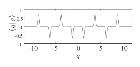
Figure 3: Position wave function of an ancilla variable, $|a\rangle$, which can be used in position quadrature error recovery.

Likewise, ancilla variables appropriate for momentum quadrature error recovery can be prepared by first squeezing the vacuum in the momentum quadrature, and replacing the qubit - continuous system interaction operator with

$$e^{-i2^{n-1}\alpha q_{e}\sigma_{z}}.$$ (33)

V Implementing in an ion trap

There are several physical systems which enable a coupling between a continuous quantum system and a discrete quantum system, such as a cavity QED system or an ion trap. Here we discuss the possibility of creating approximate encoded states in an ion trap.

Though scalable continuous variable quantum computation using ion traps seems unlikely, the ion trap provides a good test bed for such first steps as creating approximate encoded states, as the processes of decoherence within the ion trap are well understood.

Consider a single ${}^{9}\mathrm{Be}^{+}$ ion, confined in a coaxial-resonator radio frequency (RF)-ion trap, as described in Monroe et al. (1996), and references therein. The continuous quantum system is the vibrational mode of the ion, and the two-level discrete system is the ground and first excited electronic levels of the ion.

First it would be necessary to laser-cool the ion to the motional and electronic ground state, as described in Monroe et al. (1995). Ideally, we would then need to squeeze the vibrational mode of the ion. This could prove a difficult task. However, it is possible to create the sequence of operations described in Eq. (14). The Hadamard operation is accomplished by a $\pi/2$-pulse, creating an equal superposition of the ground and excited electronic states. A displacement beam is then applied which excites the motion correlated to the excited state. A $\pi$-pulse is then applied to exchange the internal states, and the displacement beam is applied again. Finally another $\pi/2$-pulse is applied, executing the second Hadamard gate. The electronic level of the ion is then measured using another laser pulse, tuned to a transition between the first excited level and a higher level. If fluorescence is observed, the ion has been measured in the $|1\rangle$ state. The absence of fluorescence indicates that the ion is in the ground state. In addition to the operations which we wish to implement, the ion trap system will undergo free evolution, so it will be necessary to couple the qubit, and measure only once every period of oscillation. In order to verify that the desired approximate encoded state had been created it would then be necessary to carry out state tomography on the system.

VI Conclusions

For a quantum computer to become a reality, the daunting task of providing adequate error correction needs to be fulfilled. At this point in time, it is unclear which, if any, implementation scheme for quantum computation will become viable. As the quantum mechanical oscillator is so prevalent in the study of quantum mechanics, it appears to be a natural test bed for quantum computation. Here we have shown how a continuous quantum system can be coupled to a discrete two level quantum system in a manner which allows the continuous quantum system to encode qubit. The ion trap provides a convenient setting for this encoding scheme as it contains the required discrete and continuous quantum variables.