Embedding dissipation and decoherence in unitary evolution schemes

Abstract

Dissipation and decoherence, and the evolution from pure to mixed states in quantum physics are handled through master equations for the density matrix. By embedding elements of this matrix in a higher-dimensional Liouville-Bloch equation, the methods of unitary integration are adapted to solve for the density matrix as a function of time, including the non-unitary effects of dissipation and decoherence. The input requires only solutions of classical, initial value time-dependent equations. Results are illustrated for a damped, driven two-level system.

The study of open quantum systems is of widespread interest across different areas of physics particularly in the irreversible processes of dissipation and decoherence afforded by coupling to an external reservoir or environment. Quantum optics is replete with such studies for optical bistability, resonance fluorescence, and the general evolution from pure to mixed states, often considered through damped, driven two-level atoms ref1 . Coupled quantum wells in a wider context and the study of quantum Brownian motion, dissipation and fluctuations have also received much attention ref2 . Application of such considerations to “quantum non-demolition” in the emerging field of laser-interferometric gravitational wave detection, and of quantum noise and decoherence in the field of quantum computation, add to the importance of this subject. Finally, this evolution from pure to mixed states is at the heart of the problem of measurement in quantum theory ref3 .

On the other hand, unitary integration schemes for the evolution operator of time-dependent Hamiltonians, when available, are powerful because they preserve invariants and are stable, also in numerical application. In this Letter, we present a general procedure and illustrate with an example how to preserve most of these advantages even while working with systems exhibiting dissipation and decoherence. There are two key steps. First, the $n$-dimensional Liouville-von Neumann-Lindblad (LvNL) equation containing dissipation and decoherence is embedded in a $(n^{2}-1)$-dimensional Liouville-Bloch form with a non-Hermitian Hamiltonian. Second, this Liouville-Bloch equation is handled by a “unitary integration” procedure that has been described in recent years ref4 ; ref5 ; ref6 wherein the evolution operator is written as a product of exponentials, each exponent involving an element of a closed Lie algebra of operators together with a multiplicative classical function of time. With all the non-commutativity handled analytically, the entire problem is reduced to solving coupled, first-order differential equations for this set of classical functions. In many cases, this set reduces to a single non-trivial Riccati (first order, quadratically nonlinear) equation for one of the classical functions, all the rest then obtained through trivial quadratures ref6 . All of the above features remain valid even when the Hamiltonian is non-Hermitian and the evolution non-unitary.

Two other papers share our aims in setting the passage from pure to mixed states in a unitary evolution scheme but they proceed differently. One deals with weak dissipation, handling the Hermitian part of the LvNL equation through unitary integration and the dissipative terms through conventional integrators ref7 . Because of their focus on numerical integration, both these handlings are for small time steps whereas we aim for integration over arbitrary, finite $t$. Another work ref8 introduces a novel “square root operator” of the density matrix and an associated $n^{2}$-dimensional Hilbert space, along with additional constraints that are not in conventional quantum mechanics. Our embedding in a higher dimensional space does not introduce any new elements beyond those already in the density matrix. After submitting our Letter, we have learnt of another work that solves master equations by invoking an “auxiliary” $n^{2}$-dimensional Hilbert space ref9 .

We begin with the master equation for the density matrix $\rho$, sometimes called the Liouville-von Neumann-Lindblad equation ref1 ; ref2 ; ref3 ,

$$i\dot{\rho} = [H,\rho]+\frac{1}{2}i\!\sum_{k}\left([L_{k}\rho,L_{k}^{\dagger}]+[L_{k},\rho L_{k}^{\dagger}]\right)$$ (1)

$$= [H,\rho]-\frac{1}{2}i\!\sum_{k}\left(L_{k}^{\dagger}L_{k}\rho+\rho L_{k}^{\dagger}L_{k}-2L_{k}\rho L_{k}^{\dagger}\right)\!,$$

where an over-dot denotes differentiation with respect to time and $\hbar$ has been set equal to unity, $H$ is a Hermitian Hamiltonian, and the second term on the right-hand side is the “Liouvillian super-operator” describing coupling to the environment and the resulting irreversibilities of dissipation and decoherence. The above form in the Markov approximation with an explicitly traceless right-hand side guarantees conservation of $Tr$($\rho$) and positivity of the probabilities. For a more mathematical description in terms of so-called “dynamical semigroups,” we refer to ref10 ; ref11 .

Our aim in this paper is to solve Eq. (1) for fairly general time-dependences of $H$ and the $L$’s contained in it, while keeping as closely as possible to the unitary integration that applies in the absence of the super-operator. This method ref4 ; ref5 ; ref6 has been developed when $H(t)$ is a sum of terms, each of which involves a time-independent operator multiplying a classical function of time. In such a case, without any recourse to time-ordered Dyson expansions, one can solve for the evolution operator $U(t)$ satisfying

$$i\dot{U}(t)=H(t)U(t),\quad U(0)=\mathcal{I},$$ (2)

by writing $U(t)$ as a product

$$U(t)=\prod_{j}\exp[-i\mu_{j}(t)A_{j}],$$ (3)

where $A_{j}$ are the operators contained in $H(t)$ together with a sequence of other operators formed out of their mutual commutators in a successive fashion. If this set forms a closed algebra under commutation, then upon substitution, Eq. (3) can be shown to satisfy Eq. (2) through repeated application of the Baker-Campbell-Hausdorff (B-C-H) identity [4,6]. This results in a well defined set of coupled first-order, generally nonlinear, equations for the functions $\mu_{j}(t).$ Thereby the quantal problem is reduced to the classical one of solving this set of equations, following which $\rho(t)$ is obtained as

$$\rho(t)=U(t)\rho(0)U^{\dagger}(t).$$ (4)

In extending this procedure to non-unitary evolution, if we were to retain only the first two terms in the superoperator, it is simple to extend Eq. (4) by using two different products $U_{L}(t)$ and $U_{R}(t)$ so that $\rho(t)=U_{L}(t)\,\rho(0)\,U_{R}^{\dagger}(t),$ with correspondingly different functions $\mu_{Lj}(t)$ and $\mu_{Rj}(t)$ in Eq. (3). Once again, upon calculating $i\dot{\rho}$ with such a form, the B-C-H identity can be used to get a well-defined set of equations for the $\mu_{L}$ and $\mu_{R}.$ However, the last term in the superoperator in Eq. (1), wherein $\rho(t)$ occurs between operators multiplying it both on the right and from the left, no longer permits easy generalization. Note that this last term is the so-called “quantum jump” in interpretations of the LvNL equation as conventional continuous evolutioni, albeit with a non-Hermitian Hamiltonian, plus a jump ref12 .

For the full master equation, we proceed by separating the invariant $Tr(\rho)$ from the $n^{2}$ elements $\rho_{ij}(t)$. Eq. (1) then reduces for the remaining $n^{2}-1$ elements to the Liouville-Bloch form

$$i\dot{\eta}(t)=\mathcal{L}(t)\eta(t),$$ (5)

where one convenient choice for the $(n^{2}-1)$ elements of $\eta$ is $\rho_{11}-\rho_{ii}$, $i=2,3,\ldots,n;$ $\rho_{ij}+\rho_{ji},$ $\rho_{ij}-\rho_{ji},$ $i>j.$ The first $(n-1)$ of these describe the diagonal elements of the density matrix, the other $(n^{2}-n)$ $i\neq j$, describe, respectively, in-phase dispersive and out-of-phase absorptive components of polarization. Even though $\mathcal{L}$ may not be Hermitian, the form of Eq. (5) is now the same as in Eq. (2) with all operators to the left of $\eta$ so that the same procedure of a product exponential form for $\eta(t)$ as in Eq. (3) can be carried out now in the $(n^{2}-1)$-dimensional space. Thereby, the LvNL equation for $\rho$ has been embedded in a higher-dimensional Liouville-Bloch equation. While invariants are no longer preserved with $\mathcal{L}$ non-Hermitian, the advantages of exponential factors, with all operator aspects handled analytically and only classical time-dependent equations to solve, still remain.

One immediate consequence is worth noting. If the operators $L_{k}$ in Eq. (1) are such that $\mathcal{L}$ in Eq. (5) involves imaginary elements and, consequently, $\eta$ decays asymptotically, $\eta(t\rightarrow\infty)\rightarrow 0$, then all coherences vanish (off-diagonal $\rho_{ij}$) and all diagonal $\rho_{ii}$ become equal, $\rho_{ii}(t\rightarrow\infty)\rightarrow(1/n)Tr(\rho(0))$. $Tr(\rho^{2})$ on the other hand, decreases asymptotically to $(1/n)$ of its initial value. A specific $n=2$ illustration will be given below of this rather general conclusion.

To demonstrate this method, we turn now to a series of recent papers ref13 that discussed phase coherences and transitions in a periodically driven two-level system with a single $L$ in Eq. (1):

$$H=\frac{1}{2}\epsilon(t)\sigma_{z}+J\sigma_{x},\;L=\sqrt{\Gamma}\sigma_{z},\;\rho_{ij}(0)=\delta_{ij}\delta_{i1}.$$ (6)

Applying our procedure, we have $\rho_{11}(t)+\rho_{22}(t)=1$, and Eq. (5) for the three remaining elements takes the form

$$i\frac{d}{dt}\left(\begin{array}[]{c}\rho_{12}+\rho_{21}\\ \rho_{21}-\rho_{12}\\ \rho_{11}-\rho_{22}\end{array}\right) = \left(\begin{array}[]{ccc}-i\Gamma&-\epsilon(t)&0\\ -\epsilon(t)&-i\Gamma&2J\\ 0&2J&0\end{array}\right)$$ (17)

$$\quad\quad\times\left(\begin{array}[]{c}\rho_{12}+\rho_{21}\\ \rho_{21}-\rho_{12}\\ \rho_{11}-\rho_{22}\end{array}\right).$$

To solve this as a product of exponentials, we need the eight operators of an SU(3) algebra. Instead, we illustrate first a simplified variant of Eq. (6) as our model, with a symmetric choice for the $L_{k}$ involving all three Pauli matrices, that is, $L_{k}=\sqrt{\Gamma/2}\sigma_{k}.$ This modifies Eq. (17) to introduce also a $(-i\Gamma)$ in the third diagonal element of the matrix. With the matrix then expressible as

$$\mathcal{L}=-i\Gamma\mathcal{I}-\epsilon(t)A_{z}+2JA_{x}\;,$$ (18)

where $A_{x}$, $A_{y}$, $A_{z}$ are the operators of angular momentum in a representation

$$A_{x}=\left(\begin{array}[]{ccc}0&0&0\\ 0&0&1\\ 0&1&0\end{array}\right) A_{y}=\left(\begin{array}[]{ccc}0&0&-i\\ 0&0&0\\ i&0&0\end{array}\right),\,$$ , (25)

$$A_{z} = \left(\begin{array}[]{ccc}0&1&0\\ 1&0&0\\ 0&0&0\end{array}\right),$$ (29)

the closed Lie algebra of these three suffices to solve Eq. (5) by our unitary integration procedure. Since this procedure rests only on the commutators between $A_{j},$ we can use any representation of them as is convenient. We exploit this in choosing Eq. (29) so that $\mathcal{L}$ involves the $A_{j}$ only linearly. Although, for comparison with ref13 , only $\epsilon$ in Eq. (18) is a function of time, we note that everything that follows applies also to more general time dependences of $J$ and $\Gamma$ and inclusion of a time-dependent term in $A_{y}$ as well. We also note that reduction of the term involving $\Gamma$ in Eq. (18) to a unit operator reflects a general sum rule in any dimension $n$. When $k$ in Eq. (1) runs over all $n^{2}$ linearly independent operators, that summation reduces to $2(n\rho_{ij}-\delta_{ij})$.

The first term in Eq. (18) leads to a trivial factor $\exp(-\Gamma t)$ and the remaining Hermitian part of $\mathcal{L}$ has been solved before ref6 :

$$\eta(t) = \exp[-\Gamma t]\exp[-i\mu_{+}(t)A_{+}]$$ (30)

$$\times\exp[-i\mu_{-}(t)A_{-}]\exp[-i\mu(t)A_{z}]\eta(0),$$

with $A_{\pm}\equiv A_{x}\pm iA_{y},$ $\eta(0)=(0,0,1),$ and

$$\dot{\mu}_{+}-i\epsilon(t)\mu_{+}-J(1+\mu_{+}^{2}) = 0,$$ (31a)

$$\dot{\mu}=2iJ\mu_{+}-\epsilon(t),$$ (31b)

$$\dot{\mu}_{-}-i\dot{\mu}\mu_{-}=J,\; \mu_{i}(0)=0.$$ (31c)

The first of these equations, involving $\mu_{+}(t)$ alone in Riccati form, is the only non-trivial member of this set. Solutions give through Eq. (30),

$$\rho_{11}(t) = \frac{1}{2}+\frac{1}{2}\exp(-\Gamma t)\,[1-2\mu_{+}(t)\mu_{-}(t)],$$

$$\rho_{22}(t) = \frac{1}{2}[1-\exp(-\Gamma t)]+\mu_{+}(t)\mu_{-}(t)\exp(-\Gamma t),$$

$$\rho_{12}(t) = i\mu_{-}(t)\exp(-\Gamma t),$$

$$\rho_{21}(t) = i\mu_{+}(t)[\mu_{+}(t)\mu_{-}(t)-1]\exp(-\Gamma t).$$ (32)

These are general solutions, valid for any time. The coherences vanish asymptotically and $\rho_{11}$ and $\rho_{22}$ attain the value $\frac{1}{2}$ as $t\rightarrow\infty$. While $Tr(\rho)$ remains always at unity, $Tr(\rho^{2})$ decreases to $(1/2)$. The above assumed as initial state the pure state with $\rho_{11}(0)=1$ the only non-zero elememt, but a wider choice also leads to the same final result. Simple numerical integration of Eq. (31a) for an oscillating driving field $\epsilon(t)=A\cos(\omega t)$ are shown in Figs. 1 and 2 for various values of the parameters $(\omega,J,A,\Gamma)$ . They are in agreement with ref13 . In Fig. 2(c), we also record the time evolution of the entropy, $S=-Tr(\rho\,\ln\,\rho)$. The value of $\Gamma$ governs the rate of rise as $S$ increases monotonically from 0 to its asymptotic limit of $\ln 2$.

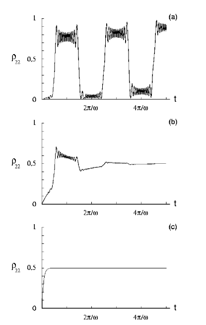
Figure 1: $\rho_{22}(t)$ for an oscillating driving field with $J/\omega=3$, $A/\omega=45$, and damping values (a) $\Gamma/\omega=0$, (b) $\Gamma/\omega=0.35$, and (c) $\Gamma/\omega=5$.

We already noted from the $3\times 3$ matrix structure of Eq. (17) that for the most general $H$ and $L$ in Eq. (6), a product of eight exponential operators always provides the requisite $\eta(t)$. As another illustration of a smaller set sufficing, when only three of the four linearly independent matrices are included in $L_{k}$, an additional inhomogeneous term in the column vector $-i\Gamma(0,0,1)$ appears on the right-hand side of Eq. (5), with $\mathcal{L}$ again as in Eq. (18). For $J=0$, this is easily solved, diagonal and off-diagonal elements decoupling, and gives the result that a mixed state evolves to the pure state (1,0).

The reduction in the number of exponential factors required is a generic feature, whenever $\mathcal{L}$ in Eq. (5) involves only the elements of a sub-algebra of the full algebra of SU($n^{2}-1$). Thus, in the $n=2$ examples considered above, the existence of SU(2) subalgebras allows solutions with just three exponential operators in Eq. (30). Denoting the eight operators of SU(3) by $O_{i},i=1-8$, with one choice for them being ($A_{z},A_{+},A_{-},A_{3}^{2},A_{+}^{2},A_{-}^{2},A_{+}A_{3}+A_{3}A_{+},A_{-}A_{3}+A_{3}A_{-}$), there are several triplets that close under commutation. These include the familiar $i=(1,2,3)$ as in Eq. (18) but also many others such as (1,5,6) and (1,7,8). There are also sub-algebras involving four (for example, (1,2,5,7) and (1,3,6,8)) and five elements (examples: (1,2,4,5,7) and (1,3,4,6,8)) in which case four or five exponential factors, respectively, would suffice for our solution in Eq. (30). As $n$ increases, although the total number of operators $n^{2}-1$ grows rapidly, once again, $\mathcal{L}$ may involve only the operators of sub-algebras, SU($n^{2}-1$) containing many sub-algebras of lower order all the way down to SU(2) with just three operators. Indeed, with increasing $n$, there are many more such sub-algebras so that very often the $H$ and $L_{k}$ may afford reduction of the number of exponentials in our procedure to a small number.

In summary, an $n$-dimensional LvNL equation describing dissipation and decoherence (or, alternatively, continuous evolution plus a quantum jump) of the density matrix $\rho(t)$ is first embedded into an ($n^{2}-1$)-dimensional Liouville-Bloch equation for diagonal and off-diagonal combinations $\eta(t)$ of $\rho(t)$. A unitary integration scheme is then applied to this form of the equation, with $\eta(t)$ expressed as a product of exponentials involving a limited, finite number of factors and operators, often just the three of angular momentum. Through this procedure, all elements of $\rho(t)$ are obtained in terms of solution of a single Riccati equation for a classical function together with ordinary multiplication and integration.

We thank Drs. Dana Browne and Lai Him Chan for suggesting we follow the entropy of evolution.

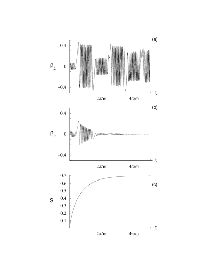
Figure 2: As in Fig. 1, for $\rho_{12}(t)$ with (a) $\Gamma/\omega=0$ and (b) $\Gamma/\omega=0.35$. The entropy $S$ for $\Gamma/\omega=0.29$ is shown in (c).

References

- (1) Email: arau@phys.lsu.edu
- (2) See, for instance, R. Bonifacio and L.A. Lugiato, in Dissipative Systems in Quantum Optics, edited by R. Bonifacio (Springer-Verlag, Berlin, 1982); D.F. Walls and G.J. Milburn, Quantum Optics (Springer-Verlag, Berlin, 1994); M.O. Scully and M.S. Zubairy, Quantum Optics (Cambridge Univ. Pr., 1996); W.P. Schleich, Quantum Optics in Phase Space (Wiley-VCH, Berlin, 2001).
- (3) See, for instance, T. Banks, L. Susskind, and M.E. Peskin, Nucl. Phys. B 244, 125 (1984); W.G. Unruh and W.H. Zurek, Phys. Rev. D 40, 107 (1989); A.J. Legget, S. Chakravarty, A.T. Dorsey, M.P.A. Fisher, A. Garg, and W. Zwerger, Rev. Mod. Phys. 59, 1 (1987); S. Gao, Phys. Rev. Lett. 79, 3101 (1997).
- (4) See, for instance, W.H. Zurek, Phys. Today 44, No. 10, 36 (1991); D. Giulini, E. Joos, C. Kiefer, J. Kupsch, I.O. Stamatescu, and H.D. Zeh, Decoherence and the Appearance of a Classical World in Quantum Theory (Springer-Verlag, Berlin, 1996).
- (5) A.R.P. Rau and K. Unnikrishnan, Phys. Lett. A 222, 304 (1996); J. Wei and E. Norman, J. Math. Phys. 4, 575 (1963); G. Campolieti and B.C. Sanctuary, J. Chem. Phys. 91, 2108 (1989).
- (6) B.A. Shadwick and W.F. Buell, Phys. Rev. Lett. 79, 5189 (1997).
- (7) A.R.P. Rau, Phys. Rev. Lett. 81, 4785 (1998) and Phys. Rev. A 61, 032301 (2000).
- (8) B.A. Shadwick and W.F. Buell, J. Phys. A 34, 4771 (2001).
- (9) B. Reznick, Phys. Rev. Lett. 76, 1192 (1996).
- (10) X.X. Yi and S.X. Yu, J. Opt. B: Quantum Semiclass. Opt. 3, 372 (2001).
- (11) G. Lindblad, Commun. Math. Phys. 48, 119 (1976); V. Gorini, A. Kassakowski, and E.C.G. Sudarshan, J. Math. Phys. 17, 821 (1976).
- (12) See, for instance, R. Alicki and K. Lendi, Quantum Dynamical Semigroups and Applications (Springer-Verlag, Berlin, 1987); E.B. Davies, Quantum Theory of Open Systems (Academic Press, London, 1976).
- (13) See, for instance, J. Dalibard, Y. Castin, and K. Molmer, Phys. Rev. Lett. 68, 580 (1992); H.J. Carmichael, An Open Systems Approach to Quantum Optics (Springer-Verlag, Berlin, 1993).
- (14) Y. Kayanuma, Phys. Rev. B 47, 9940 (1993); Y. Kayanuma and Y. Mizumoto, Phys. Rev. A 62, 061401 (2000); K. Saito and Y. Kayanuma, Phys. Rev. A 65, 033407 (2002).