2D Ising Model with non-local links - a study of non-locality

Abstract

Markopoulou and Smolin have argued that the low energy limit of LQG may suffer from a conflict between locality, as defined by the connectivity of spin networks, and an averaged notion of locality that emerges at low energy from a superposition of spin network states. This raises the issue of how much non-locality, relative to the coarse grained metric, can be tolerated in the spin network graphs that contribute to the ground state. To address this question we have been studying statistical mechanical systems on lattices decorated randomly with non-local links. These turn out to be related to a class of recently studied systems called small world networks. We show, in the case of the 2D Ising model, that one major effect of non-local links is to raise the Curie temperature. We report also on measurements of the spin-spin correlation functions in this model and show, for the first time, the impact of not only the amount of non-local links but also of their configuration on correlation functions.

2005 number number identifier [dated: ]Oct. 30, 2005

In loop quantum gravity (LQG), states are described by spin networks, from which non-local (NL) links can emerge due to the mismatch of micro-locality and macro-localityMarkopoulou2004 Smolin2005con Smolin2005 . In other words, two nodes which are local microscopically in the fundamental graph can turn out to be macroscopically far away from each other and connected by a NL link relative to the coarse grained metric. Ends of the NL links carrying gauge field representations may be interpreted as gauge particles, while the ends of those carrying no gauge fields can be some unknown neutral particles and hence serve as a type of source of dark matterSmolin2005con Smolin2006 . It is found that the MOND force law may also be recovered on a regular Euclidean lattice randomly decorated with some NL links characterized by some distribution function $P(r)$, which is the probability of having a NL link between two nodes separated by a distance $r$ measured by the regular lattice metricSmolin2005 . Since NL links correlate the fields at randomly chosen far away points without violating the local conservation of averaged energy, they may explain the non-locality in quantum physics and moreover, the origin of quantum physics according to Nelson’s formalism of stochastic quantum theoryMarkopoulou2004 Smolin2005 .

To address these questions, we study the statistical behavior of 2D Ising models, with randomly added NL links. Such a system is related to a class of recently studied systems—small world networks (SWN), which are very useful in describing many interesting social systems, such as railway network and disease spreadingWatts1998 Kleinberg2002 Newman1999 . However, our approach and focus in this letter are different from those for the SWN in that 1) we add a given number of NL links randomly to the regular lattice with uniform distribution probability, and 2) we study and find the effects of not only the amount of NL links but also the configuration of NL links on the system’s behavior, especially on correlation functions, which are tightly related to the system’s dynamics. To do so, we use Monte Carlo simulation.

.1 Simulation of 2D Ising Spin System with Random NL links

We adopt Metropolis Monte Carlo method and apply periodic boundary condition. We mainly simulate a $20\times 20$ 2D square ferromagnetic Ising model randomly decorated with NL links based on the uniform distribution probability. Note that rewiring is not allowed and any two spins cannot be directly connected by more than one link. We take the interaction coupling, $J=-1,$ and Boltzman constant, $k_{B}=1,$ such that all the quantities presented are dimensionless. The spin-spin correlation function $g\left(r\right)$ needs some clarification. We study the pair correlation of the system as a function of $r$, defined as the minimum number of links connecting one spin to another. Because non-local links break the symmetry of the lattice, $g\left(r\right)$ should be obtained, for each $r$, by doing both ensemble average and the average over the number of pairs of spins with the same distance $r$. Mathematically, this is described by

$$g\left(r\right)=\sum\limits_{\left(i,j\right)_{r}}\left[\left\langle\sigma_{i}\sigma_{j}\right\rangle_{r}-\left(\left\langle\sigma_{i}\right\rangle\left\langle\sigma_{j}\right\rangle\right)_{r}\right]/\#\text{pairs}\left(i,j\right)_{r},$$

where the $\left\langle{}\right\rangle$ denotes ensemble average, the subscript $r$ denotes the distance between two spins in the pair, and $\#$ means ”the number of”.

.2 Effects of the Amount of NL links

Since we assume a uniform distribution probability for the NL links, the only control we have on NL links is the number of them. Therefore, it is natural to look at the effects of NL links on the system’s behavior by varying their number.

Fig. (1) compares five curves, which correspond to the specific heat of a $20\times 20$ regular lattice with respectively $0$, $10$, $20$, $50$ and $100$ NL links. One can see the increase of the critical temperature with the number of NL links. This is so because, for a finite system, adding NL links effectively increases the dimensionality of the lattice and of course the average valence of the nodes. This argument can also be verified by noticing the decrease of the peak height as the number of NL links increases. Due to the finite scaling effect, the peak rises with the system size, $L$, defined by $L^{D}=N$, where $N$ is the number of nodes of the system and $D$ is the dimension. Now that $D$ increases with the amount of NL links, but with $N$ fixed, $L$ must decrease and so does the peak height. The last effect shown in the plot is that the half width of the $C_{V}$-curve also increases with the amount of NL links. This is understood by noting that 1) the system with NL links has more states and 2) there are more non-frozen states in the region of $T<T_{c}$ as $T_{c}$ increases with the amount of NL links.

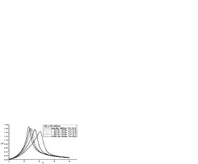
Figure 1: $C_{V}$-curves of respectively a regular $20\times 20$ Ising spin system, the same system with $10$, $20$, $50$, and $100$ non-local links. The data of this plot is from Dr. Lixin Zhan with Wang-Landau method.

Similar results are reported for SWNs on Ising model by Cai et. al.Cai2004 , by HerreroHerrero2002 , and by HastingsHastings2003 .

Figure 2: Plot of $T_{c}/N$ versus $N$, the system size, in the case of total connectedness.

One may ask if there is an upper limit of the critical temperature when we keep adding NL links. Yes, there is a maximum $T_{c}$, which is the very critical temperature in the extreme case when the system is totally connected. In the stage of total connectedness, $T_{c}$ raises with the system size, which is now equal to $N$. This is illustrated in Fig. (2), where $T_{c}/N$ is asymptotic to unity in the limit of $N\rightarrow\infty$. One can locate $T_{c}=364$ for a totally connected system of $400$ spins (having $79800$ links), which corresponds to a $20\times 20$ regular Ising system with $79000$ NL links. This also implies that $T_{c}$, after a very short linear range, increases slower and slower to approach the maximally allowed $T_{c}$.

It is more interesting to see how the system’s correlation function behaves in the presence of NL links. Fig. (3) shows three pairs of correlation functions, each of which contains one for a regular lattice and one for the same lattice with $20$ NL links. The upper pair compares the two at their critical temperatures, one at $T_{c}=2.3$ and one at $T_{c}^{\prime}=2.5$ due to NL links. One can see that both $g\left(r\right)$’s behave similarly and indicate correlation lengths of the order of $L$, although with different decay rates. By getting rid of the boundary effect, we have $g\left(r\right)\propto r^{-0.2188}$ for the regular lattice, and $g\left(r\right)\propto r^{-0.2996}$ for the one with $20$ NL links. In the middle pair where each one is at a temperature of $0.2$ above its own critical temperature, the two $g\left(r\right)$’s are closer to each other and give rise to correlation lengths of the order of $L$, because the system is finite and is in the vicinity of phase transition. However in this case, one will see in the next section that there is some subtlety for the correlation function of the system with NL links. In the lower pair where each one is at a temperature of $0.4$ below its own critical temperature, the two $g\left(r\right)$’s are almost the same and this is consistent with the fact that the correlation length should be finite at such temperatures. Therefore, even when the system is decorated with NL links, the number of which is comparable to $L$, its correlation function is different but does not deviate very much from that of the regular lattice.

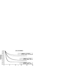
Figure 3: Comparison between the correlation function of the regular $20\times 20$ Ising model and that of the same lattice with $20$ non-local links randomly distributed.

.3 Effects of the Configuration of NL links

So far we just add, at the beginning of each run of the simulation, a certain number of NL links on the lattice randomly based on the uniform distribution probability, without any further control of their locations in the lattice. Consequently, we may have different configurations of NL links on the lattice in different runs of the simulation with all other parameters fixed. Now, let us check if the configuration of NL links in the lattice has any impact on the system’s behavior.

Actually, when the number of NL links is fixed, the $C_{V}$-curve is self-averaging. This is verified by simulation. As an illustration, Fig. (4) plots ten $C_{V}$-curves of ten runs (arbitrarily taken from hundreds of runs) of the simulation with different NL link configuration but with all other parameters the same. One can observe that all $C_{V}$-curves coincide very well and peak at the same $T_{c}$. This suggests that for a system, $C_{V}$ and hence $T_{c}$ are only sensitive to the total number of links (both regular and NL links) on the lattice. The reason is that $C_{V}$ is a first order derivative of system’s energy with respect to temperature and the energy is only related the total number of links on the Ising lattice with nearest neighbor interaction.

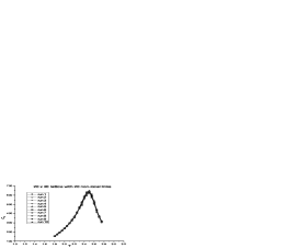
Figure 4: comparison of $C_{V}$ curves at $10$ runs of simulation with all parameters the same except the configuration of non-local links.

Nevertheless, if we look at the correlation function at temperatures not so far from the critical temperature, configuration of NL links does effect. Recall that we mentioned the subtlety of the correlation function of a $20\times 20$ lattice with $20$ NL links. This is illustrated in Fig. (5), where we compare correlation functions at $T=2.3$ from $20$ runs (taken from hundreds of runs) of the simulation with different NL link configuration but with the same parameters. The system is in the vicinity of the phase transition, since $T_{c}\approx 2.5$ in this case. Nineteen $g\left(r\right)$’s of them are similar in that they all indicate a correlation length of the order of $L$, with although different speed of falling off. We call them normal ones in the sense that they behave similar to the correlation function of the regular lattice at $T$ of the same distance from the regular $T_{c}$. However, one of them, namely the special one, falls off to zero rapidly and hence gives short correlation length of the system. This is indeed due to a special configuration of the NL links on the lattice. We show $20$ $g\left(r\right)$’s in this figure, because the ratio of the special one to the normal one is roughly between $1/30$ and $1/20$.

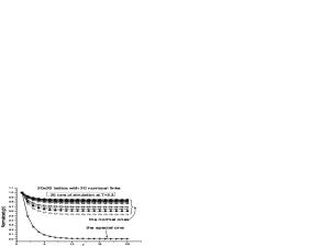
Figure 5: Comparison of correlation functions at $T=2.3$, which are obtained from $20$ runs of simulation with same parameters, of a $20\times 20$ Ising lattice with $20$ non-local links.

Fig. (6) presents two different typical configurations of the $20$ NL links on the $20\times 20$ lattice. The configuration corresponding to the special correlation function in Fig. (5) is shown in Fig. (6a) (type A), where one can see that the whole upper left quarter of the lattice has virtually no NL links. On the other hand, the configuration in Fig. (6b) (type B), which corresponds to a typical one of the $19$ normal correlation functions, shows a much more evenly distribution of NL links. By doing many simulations, we found that the length $l$ of NL links, measured by the number of regular links taken from one end to the other end of the NL link, are statistically different in the two cases. For special ones, $l_{\min}\geq 5$, and $l_{\mathrm{avg}}\geq 10$, where $l_{\min}$ is the minimum length and $l_{\mathrm{avg}}$ is the averaged $l$ over the number of configurations of the same type. But in the normal cases, we have $2\leq l_{\min}\leq 4$ and $l_{\mathrm{avg}}\leq 10$. Based on these observations, this phenomenon can be explained as follows. Since we choose the uniform distribution probability of the NL links, in most of the cases one should obtain configurations of NL links of type B; this explains why there are more normal correlation functions than the special ones. In type B configurations, NL links are short and very evenly distributed, so their effect on the correlation function is well averaged out. As a consequence, the system is correlated as there are no many NL links although $T_{c}$ is different. Whereas, in type A configurations, NL links are longer and packed in some region of the lattice. Provided this is so, the region where NL links gather are effectively a sub-system of much higher dimension with of course a much higher $T_{c}^{\prime}$, then the correlation function of this sub-system behaves as at a temperature much below $T_{c}^{\prime}$ and gives rise to short correlation length as it should. Moreover, the effect of NL links can hardly be averaged out in such cases. Therefore, one sees the special correlation functions.

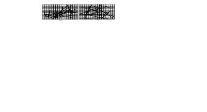
Figure 6: Two configurations of $20$ non-local links on a $20\times 20$ lattice: (a) configuration corresponding to the special correlation function in fig. (5); (b) configuration corresponding to a normal correlation function in fig. (5).

.4 Conclusions and Future Works

We conclude that 1) the Curie temperature of the system increases with the amount of NL links; 2) the Curie temperature is not sensitive to the configuration of NL links; 3) normally, correlation functions of systems with NL links behave similarly to those of regular lattices, with noticeable difference in the decay rate; and 4) there exist some special cases where the correlation functions of systems with NL links behave very differently from regular ones due to some underlying special configurations of NL links on lattices. Although it is hard to exclude the boundary effect due to the small size of the systems we studied, the above results can still be valid for large systems, especially when we are only interested in the physics in some portion of the whole system. Nevertheless, to study large systems is of course demanding and is one of our next steps. Conclusions one and two suggest some manipulation of the interactions $J$ in the model, because $C_{V}$-curves and $T_{c}$ will be subject to the configurations of NL links if we choose a distance dependent interaction $J\left(r\right)$. Conclusions three and four, on the other hand, suggest a modification on the distribution probability $P\left(r\right)$ of the NL links. We see that correlation functions suffer from the configuration of NL links, so we may get a special type of correlation functions by controlling the configuration of NL links through a well designed $P\left(r\right)$. For example, we may take a $J\left(r\right)$, which has been studied by others and has physical significance for a square spin lattice, and then look for a $P\left(r\right)$ with the above property. This would imply that a physical system dominated by some interaction law can be equivalent to a system with non-local links, which however obeys a much simpler interaction law. Some of these may be done analytically. We can also extend the study to more complicated lattice systems, or even to spin networks in the future.

Acknowledgements—The author specially thanks Prof. Lee Smolin, the author’s supervisor, for his intuitions, discussions and comments. The author thanks Dr. Lixin Zhan for checking some of the results. Thanks also go to Mohammed Ansari, Doug Hoover, and Prof. Maya Paczuski and their useful comments and discussions. The author would like to thank NSERC for the financial support.

References

- (1) F. Markopoulou and L. Smolin, Phys. Rev. D70, 124029 (2004), see also: gr-qc/0311059.
- (2) L. Smolin, Loops’05, Potsdam, Germany, Oct., 2005, http://loops05.aei.mpg.de/index_files/abstract_smolin.html.
- (3) F. Markopoulou and L. Smolin, In Preparation.
- (4) S. O. Bilson-Thompson , F. Markopoulou and L. Smolin, In preparation.
- (5) D. J. Watts and S. H. Strogatz, Nature 393, 440 (1998).
- (6) T. G. Dietterich, S. Becker, and Z. Ghahramani, eds., Small-World Phenomena and the Dynamics of Information, NIPS (MIT Press, Cambridge, MA, 2002).
- (7) M. E. J. Newman and D. J. Watts, Phys. Rev. E 60, 7332 (1999).
- (8) T.-Y. Cai and Z.-Y. Li, Intl. J. of Mod. Phys. B 18, 2575 (2004).
- (9) C. P. Herrero, Phys. Rev. E 65, 066110 (2002).
- (10) M. B. Hastings, Phys. Rev. Lett. 91, 098701-1(2003).