Abstract

The string effective action at tree level contains, in its bosonic sector, the Einstein-Hilbert term, the dilaton, and the axion, besides scalar and gauge fields coming from the Ramond-Ramond sector. The reduction to four dimensions brings to scene moduli fields. We generalize this effective action by introducing two arbitrary parameters, $\omega$ and $m$, connected with the dilaton and axion couplings. In this way, more general frameworks can be analyzed. Regular solutions with a bounce can be obtained for a range of (negative) values of the parameter $\omega$ which, however, exclude the pure string configuration ($\omega=-1$). We study the evolution of scalar perturbations in such cosmological scenarios. The predicted primordial power spectrum decreases with the wavenumber with spectral index $n_{s}=-2$, in contradiction with the results of the $WMAP$. Hence, all such effective string motivated cosmological bouncing models seem to be ruled out, at least at the tree level approximation.

Pacs numbers: 04.20.Cv., 04.20.Me,98.80.Cq

1 Introduction

The standard cosmological model, based on the general relativity theory, has been successfully tested until the nucleosynthesis era, around $t\sim 1\,s$, that is, at $T\sim 1\,MeV$[1, 2]. At times before this era, it is only possible to speculate on how the universe has behaved. There are some claims that the spectrum of the anisotropy of the cosmic microwave background radiation (CMBR) has allowed to test the inflationary scenario, opening a window to energy levels of about $10^{15}\,GeV$[3, 4, 5]. However, this last statement remains controversial[6]: there is not, at this moment, a unique, complete, inflationary model, free of problems like transplanckian frequencies and fine tuning of fundamental parameters. In this sense the inflationary model remains a theoretical proposal asking for a full consistent formulation. Moreover, the fitting of the CMBR spectrum is made through a quite large number of parameters (up to ten), and more results, like the identification of the gravitational waves contribution to the CMBR anisotropy through the full detection of the polarization parameters of the CMB photons are necessary in order to surmount the degeneracy in the parameter space. Finally, neither the standard cosmological model nor the inflationary scenario address the question of the initial singularity, which is a major problem in the primordial cosmology. Hence, the very early universe remains an open area of research.

String theory[7] is, at the moment, the most important candidate to a fundamental theory of nature unifying all interactions including gravity. At very low energy levels, string theory reduces to general relativity in its gravity sector. On the other hand, at higher energies, it predicts a deviation from the general relativity framework: the dilaton field couples non-minimally to the Einstein-Hilbert term; the Neveu-Schwarz sector exhibits also an axion field, which in four dimensions is equivalent to a scalar field which couples with the dilaton; in the Ramond-Ramond sector, scalar fields and gauge fields, minimally coupled to gravity and to the dilaton field, are present. Moreover, string theory is formulated in ten dimensions, and the reduction to four dimensions leads to the appearance of moduli fields associated with the dynamics of the extra dimensions. String theory itself may be incorporated in a more fundamental structure in $11$ dimensions ($M$ theory), $12$ dimensions ($F$ theory) and so on. All these complex structures lead, in principle, to a strong deviation from the standard cosmological scenario at very high energies.

The question we address here is how such a rich structure affects the evolution of the universe in its primordial phase. This problem has already been studied in many aspects in the literature[10]. The pre-big bang scenario[11], the ekpyrotic model[12], and the string gas cosmology [13] are some of them. However, all these attempts are plagued with some important difficulties: to construct a completely regular cosmological scenario, without any kind of singularity, which consequences can be successfully tested against observation.

General scalar-tensor systems which reduce to the particular string effective action for some values of the free parameters, have been considered in the literature [14, 15, 16]. In reference [14], a $D$ dimensional lagrangian has been analyzed, with two free parameters $\omega$ and $m$, which are connected with the coupling of the dilaton and the axion fields, respectively. The original configuration has been compactified considering flat, static extra dimensions. For a specific range of values of $\omega$, scenarios with no curvature singularity have been obtained. However, the dilaton field is null initially, pointing out a singularity in the string expansion parameter, and thus rendering the effective model inadequate at that moment. In reference [15] fields from the Ramond-Ramond sector have been considered. This allows to avoid the singularity in the string expansion parameter, but only in the case of large negative values of $\omega$, that is, $\omega<-3/2$. This implies the presence of negative energies when the lagrangian is re-expressed in the Einstein frame. The $D$ dimensional structure has been studied, in the vacuum case, in reference [16] and regular solutions have been obtained, again for large negative values $\omega$.

In the present work, we perform a two-fold analysis. First, we explore another possibility with respect to some previous works (mainly references [14, 15]): we take into account the dynamics of the extra dimensions, and a radiative fluid whose presence is suggested by a maxwellian field in the Ramond-Ramond sector. Again, completely regular models can be obtained, this time for a larger range of values of the parameter $\omega$, mainly with respect to the results of reference [15]: this parameter must still be negative, but in four dimensions it can be greater than $-3/2$. The pure string case, which is characterized by $\omega=-1$, still leads to scenarios which are not completely regular; in fact this particular value can imply regularity only when the number of extra dimensions goes to infinity. On the other hand, even if $\omega<-1$, there are possible connections between $M$ and $F$ theories. We describe the features of these models, which display a bounce in the scale factor, while the dilaton and the moduli fields remain regular. We then test the new scenario obtained here against observations, as well as those obtained in [14, 15], by computing the spectrum of scalar perturbations. The general result is that these models predict a decreasing power spectrum, which disagrees strongly with observations[17]. As a general feature, all the scenarios lead to a spectral index for scalar perturbations that is around $-2$. This means that it is not possible to construct a realistic regular cosmological scenario based on the string (and more general frameworks) effective action at tree level unless, perhaps, some non trivial compactification scheme is introduced, or more complex configurations are considered like, for example, the (condensate) fermionic terms.

In the next section we describe the construction of the effective action. In section $3$, the background solutions are obtained. In section $4$ a perturbative analysis is carried out for the scalar modes and the power spectrum is computed. In section $5$ we present our conclusions.

2 The effective action in four dimensions

Our starting point is the string effective action in $D$ dimensions at tree level coupled to a radiative field:

$$L=\sqrt{-\tilde{g}}e^{-\sigma}\biggr{\{}\tilde{R}-\tilde{\omega}\sigma_{;A}\sigma^{;A}-\frac{1}{12}H_{ABC}H^{ABC}\biggl{\}}-\sqrt{-\tilde{g}}\frac{\xi_{;A}\xi^{;A}}{2}+L_{matter}\quad,$$ (1)

where $A,B,C=1,...,D$, $\sigma$ is the dilatonic field, $H_{ABC}$ is the axionic field, $\xi$ is a scalar field coming from the Ramond-Ramond sector and $L_{matter}$ represents the matter lagrangian, in this case a radiative fluid. The origin of the radiative fluid may be traced back to electromagnetic terms present in the Ramond-Ramond sector. In the pure string case, $\tilde{\omega}=-1$, but other values of $\tilde{\omega}$ are allowed if the effective action (1) is obtained from a fundamental theory in higher dimensions, like M-theory or F-theory. In these cases, the value of $\tilde{\omega}$ can be different from $-1$; in particular it can be largely negative [15].

The $D$-dimensional metric describes now a manifold decomposition $M^{4}\times V^{D-4}$, where $M^{4}$ is a four-dimensional space-time and $V^{D-4}$ is an internal space which is supposed to be flat. The line element takes the form

$$ds^{2}=g_{\mu\nu}dx^{\mu}dx^{\nu}-e^{2\beta}dy^{i}dy_{i}\quad,$$ (2)

where $\mu,\nu=1,...4,$ and $i=1,...,D-4$, with $\beta$ depending only on $x^{\mu}$. In this case, the Ricci scalar in $D$ dimensions is

$$\tilde{R}=R-2d\Box\beta-d(d+1)\beta_{;\rho}\beta^{;\rho}\quad,$$ (3)

with $d=D-4$, and $R$ being the scalar curvature in 4-dimensions. The reduced lagrangian in four dimension reads,

$$L = \sqrt{-g}e^{d\beta-\sigma}\biggr{\{}R-2d\Box\beta-d(d+1)\beta_{;\rho}\beta^{\rho}-\tilde{\omega}\sigma_{;\rho}\sigma^{;\rho}-\frac{1}{12}H_{\mu\nu\lambda}H^{\mu\nu\lambda}\biggl{\}}$$ (4)

$$- \sqrt{-g}e^{d\beta}\frac{\xi_{;\rho}\xi^{;\rho}}{2}+L_{matter}\quad,$$

where we have supposed that the axion field $H_{ABC}$ and $\sigma$ also depend only on $x^{\mu}$. Defining $\phi=e^{d\beta-\sigma}$, and performing integration by parts in the second term of (4) the lagrangian reduces to

$$L = \sqrt{-g}\phi\biggr{\{}R-\biggr{[}d(d+1)+\tilde{\omega}d^{2}\biggl{]}\beta_{;\rho}\beta^{\rho}-\tilde{\omega}\frac{\phi_{;\rho}\phi^{;\rho}}{\phi^{2}}$$ (5)

$$+ 2d(1+\tilde{\omega})\beta_{;\rho}\frac{\phi^{;\rho}}{\phi}-\phi^{-2}\Psi_{;\rho}\Psi^{;\rho}\biggl{\}}$$

$$- \sqrt{-g}e^{d\beta}\frac{\xi_{;\rho}\xi^{;\rho}}{2}+L_{matter}\quad.$$

The axion field has been written as $H^{\mu\nu\nu}=\phi^{-1}\epsilon^{\mu\nu\lambda\gamma}\Psi_{;\gamma}$. The final form of the lagrangian is

$$L = \sqrt{-g}\phi\biggr{\{}R+\gamma_{;\rho}\gamma^{;\rho}-\omega\frac{\phi_{;\rho}\phi^{;\rho}}{\phi^{2}}-\phi^{m-1}\Psi_{;\rho}\Psi^{;\rho}\biggl{\}}$$ (6)

$$- \sqrt{-g}\phi^{-\frac{ds}{r}}e^{\frac{d}{r}\gamma}\frac{\xi_{;\rho}\xi^{;\rho}}{2}+L_{matter}\quad,$$

where we have defined $\gamma=r\beta+s\ln\phi$ with $r^{2}=-[d(d+1)+\tilde{\omega}d^{2}]$ and $s=d(1+\tilde{\omega})/r$. The parameter $\omega$ is given by

$$\omega=-\frac{(d-1)\tilde{\omega}+d}{d(1+\tilde{\omega})+1}\quad.$$ (7)

In this effective lagrangian, we have introduced an arbitrary constant $m$ in the coupling between the dilaton and axion field. In the pure string case, $m=-1$ and $\omega=-1$. However, in what follows, we will keep $m$ and $\omega$ arbitrary in order to have contact with general multidimensional and supergravity theories, as well as some extensions of the string theory, like $M$ or $F$ theories. Notice that $\tilde{\omega}=-1$ implies $\omega=-1$. Hence, the traditional string configuration is a kind of fixed point. The form of the lagrangian (6) is valid under the condition $\tilde{\omega}<-(d+1)/d$ ($r$ is real). This excludes the strict string case, but it includes $\tilde{\omega}>-3/2$. The consequences of supposing $\tilde{\omega}>-(d+1)/d$ (which amounts to change the sign of the term in $\gamma$) will be discussed later.

From (6), the field equations read:

$$R_{\mu\nu}-\frac{1}{2}g_{\mu\nu}R = \frac{8\pi}{\phi}T_{\mu\nu}+\frac{\omega}{\phi^{2}}\biggr{(}\phi_{;\mu}\phi_{;\nu}-\frac{1}{2}g_{\mu\nu}\phi_{;\rho}\phi^{;\rho}\biggl{)}$$ (8)

$$+ \frac{1}{\phi}\biggr{(}\phi_{;\mu;\nu}-g_{\mu\nu}\Box\phi\biggl{)}-\biggr{(}\gamma_{;\mu}\gamma_{;\nu}-\frac{1}{2}g_{\mu\nu}\gamma_{;\rho}\gamma^{;\rho}\biggl{)}$$

$$+ \phi^{m-1}\biggr{(}\Psi_{;\mu}\Psi_{;\nu}-\frac{1}{2}g_{\mu\nu}\Psi_{;\rho}\Psi^{;\rho}\biggl{)}$$

$$+ \frac{\phi^{-\frac{ds}{r}-1}e^{\frac{d}{r}\gamma}}{2}\biggr{(}\xi_{;\mu}\xi_{;\nu}-\frac{1}{2}g_{\mu\nu}\xi_{;\rho}\xi^{;\rho}\biggl{)}\quad;$$

$$\Box\phi+\frac{1-m}{3+2\omega}\phi^{m}\Psi_{;\rho}\Psi^{;\rho} + \frac{1}{3+2\omega}\biggr{(}\frac{ds}{r}+1\biggl{)}\phi^{-\frac{ds}{r}}e^{\frac{d}{r}\gamma}\frac{\xi_{;\rho}\xi^{;\rho}}{2}$$ (9)

$$= \frac{8\pi}{3+2\omega}T\quad;$$

$$\Box\Psi+m\frac{\phi^{;\rho}}{\phi}\Psi_{;\rho} = 0\quad;$$ (10)

$$\Box\gamma+\frac{\phi^{;\rho}}{\phi}\gamma_{;\rho}+\frac{1}{4}\frac{d}{r}\phi^{-\frac{ds}{r}-1}e^{\frac{d}{r}\gamma}\xi_{;\rho}\xi^{;\rho} = 0\quad;$$ (11)

$$\Box\xi-\frac{ds}{r}\frac{\phi_{;\rho}\xi^{;\rho}}{\phi}+\frac{d}{r}\gamma_{;\rho}\xi^{;\rho} = 0\quad;$$ (12)

$${T^{\mu\nu}}_{;\mu} = 0\quad.$$ (13)

The energy-momentum tensor has the perfect fluid form $T^{\mu\nu}=(\rho+p)u^{\mu}u^{\nu}-pg^{\mu\nu}$.

3 Regular cosmological solutions

Let us consider a homogeneous and isotropic space-time described by the Friedmann-Robertson-Walker metric

$$ds^{2}=dt^{2}-a^{2}(t)\biggr{\{}\frac{dr^{2}}{1-kr^{2}}+r^{2}(d\theta^{2}+\sin^{2}\theta d\phi^{2})\biggl{\}}.$$ (14)

As usual, $a(t)$ is the scale factor, and $k=-1,0,1$ represents the normalized curvature of the spatial section. Inserting the metric in the field equations, we obtain the following equations of motion:

$$3\biggr{(}\frac{\dot{a}}{a}\biggl{)}^{2}+3\frac{k}{a^{2}} = \frac{8\pi}{\phi}\rho+\frac{\omega}{2}\biggr{(}\frac{\dot{\phi}}{\phi}\biggl{)}^{2}-3\frac{\dot{a}}{a}\frac{\dot{\phi}}{\phi}-\frac{\dot{\gamma}^{2}}{2}+\frac{\phi^{m-1}}{2}\dot{\Psi}^{2}$$ (15)

$$+ \frac{\phi^{-\frac{ds}{r}-1}e^{\frac{d}{r}\gamma}}{4}\dot{\xi}^{2}\quad,$$

$$\ddot{\phi}+3\frac{\dot{a}}{a}\dot{\phi}+\frac{1-m}{3+2\omega}\phi^{m}\dot{\Psi}^{2} + \frac{1}{3+2\omega}\biggr{(}\frac{ds}{r}+1\biggl{)}\phi^{-\frac{ds}{r}}e^{\frac{d}{r}\gamma}\frac{\dot{\xi}^{2}}{2}$$ (16)

$$= \frac{8\pi}{3+2\omega}(\rho-3p)\quad,$$

$$\ddot{\Psi}+3\frac{\dot{a}}{a}\dot{\Psi}+m\frac{\dot{\phi}}{\phi}\dot{\Psi} = 0\quad,$$ (17)

$$\ddot{\gamma}+3\frac{\dot{a}}{a}\dot{\gamma}+\frac{\dot{\phi}}{\phi}\dot{\gamma}+\frac{1}{4}\frac{d}{r}\phi^{-\frac{ds}{r}-1}e^{\frac{d}{r}\gamma}\dot{\xi}^{2} = 0\quad,$$ (18)

$$\ddot{\xi}+3\frac{\dot{a}}{a}\dot{\xi}-\frac{ds}{r}\frac{\dot{\phi}}{\phi}\dot{\xi}+\frac{d}{r}\dot{\gamma}\dot{\xi} = 0,$$ (19)

$$\dot{\rho}+3\frac{\dot{a}}{a}(\rho+p) = 0\quad.$$ (20)

It will be supposed that the ordinary fluid obeys a barotoropic equation of state, $p=\alpha\rho$, with $-1\leq\alpha\leq 1$.

Equations (17,19,20) admit the first integrals

$$\dot{\Psi}=A\frac{\phi^{-m}}{a^{3}}\quad,\quad\dot{\xi}=\xi_{0}\frac{\phi^{\frac{ds}{r}}e^{-\frac{d}{r}\gamma}}{a^{3}}\quad,\quad\rho=\rho_{0}a^{-3(1+\alpha)}\quad,$$ (21)

where $A$, $\xi_{0}$ and $\rho_{0}$ are integration constants. In the absence of the RR field $\xi$, equation (18) admits also a first integral given by

$$\dot{\gamma}=\frac{B}{a^{3}\phi}\quad,$$ (22)

where $B$ is a constant

In the absence of the moduli field, the equation for the RR field is obtained from Eq. (5) by making $\beta=$const. and absorving $\exp(d\beta)$ in the definition of $\xi$, yielding $\Box\xi=0$ with solution $\dot{\xi}=\xi_{0}/a^{3}$.

It seems that there exists no general closed solution when all fields are taken into account. However, particular cases can be explicitly solved. The solutions without the moduli fields were found in reference [15]; the main scenarios for this case will be reviewed below. The equations, in the presence of moduli fields, but in the absence of the Ramond-Ramond (RR) term, will be solved for two main cases: in the absence of the axion field, and in the presence of the axion field. Only the flat case will be treated. The final conclusions may also be applied to the non flat cases.

3.1 Solutions in absence of the moduli fields

When the internal scale factor is static, regular solutions, with no divergence in the dilaton field and the space-time curvature, are obtained both in the absence of the RR scalar field and in the presence of the RR scalar field. For both cases, the coupling constant $\omega$ must be smaller than $-3/2$ in order to obtain a completely regular scenario. This means that in the Einstein frame, negative energies are present. The flat solutions of interest were obtained in reference [15]. They are the following:

• Pure anomolous axionic case ($\omega<-3/2,m=-1$):

  $$a(\tau) = \frac{a_{0}}{\sqrt{\sinh\alpha\tau}}\biggr{[}1-\sin f(\tau)\biggl{]}^{-1/2}\quad,$$ (23)

  $$\phi(\tau) = \phi_{0}\sinh(\alpha\tau)\quad,$$ (24)

  $$\Psi^{\prime} = A\phi\quad,$$ (25)

  $$f(\tau) = \ln\biggr{[}\biggr{|}\tanh\biggr{(}\frac{\alpha\tau}{2}\biggl{)}\biggl{|}^{p}\biggl{]}\quad,$$ (26)

  where

  $$\alpha=\sqrt{\frac{-2A^{2}}{3+2\omega}}\quad,\quad p=\pm\sqrt{-\biggr{(}1+\frac{2}{3}\omega\biggl{)}}\quad,$$

  $$a_{0}^{2}=\frac{A^{2}\phi_{0}}{3M}\quad,\quad M=\frac{8\pi\rho_{0}G}{3c^{2}}$$ (27)

  where $A$ is a constant. The time parameter $\tau$ is related to the cosmic time $t$ by the relation $dt=a^{3}d\tau$ and a prime means derivative with respect to $\tau$.

• Anomolous RR case ($\omega<-3/2,m=-1$):

  $$a(\tau) = \frac{a_{0}}{\sqrt{\sinh(\alpha\tau)-s_{0}}}\biggr{[}1-\sin f(\tau)\biggl{]}^{-1/2}\quad,$$ (28)

  $$\phi = \phi_{0}[\sinh(\alpha\tau)-s_{0}]\quad,$$ (29)

  $$\Psi^{\prime} = A\phi\quad,$$ (30)

  $$\xi = \chi_{0}={\rm const.}\quad,$$ (31)

  $$f(\tau) = p\ln\biggr{|}\frac{2}{s_{0}}\biggr{[}\frac{s_{0}\tanh(\alpha\tau/2)+1-\sqrt{1+s_{0}^{2}}}{1+\sqrt{1+s_{0}^{2}}+s_{0}\tanh(\alpha\tau/2)}\biggl{]}\biggl{|}\quad,$$ (32)

where now

$$a_{0}^{2}=\frac{A^{2}\phi_{0}}{3M}(1+s_{0}^{2})\quad{\rm and}\quad s_{0}=\frac{\xi_{0}^{2}}{2A^{2}\phi_{0}}>1.$$ (33)

In the two cases there are bounces in the scale factor. One can be obtained by choosing $\tau_{i}$ and $\tau_{f}$ such that $f(\tau_{i})=-7\pi/2$ and $f(\tau_{f})=-3\pi/2$. It represents an asymptotically radiation dominated universe contracting from infinity which bounces at $\tau_{B}$ such that $f(\tau_{B})=-5\pi/2$, expanding aterwards to another asymptotically radiation dominated phase. The dilaton is always finite, going from $\phi_{i}/\phi_{0}=10^{-1}$ to $\phi_{f}/\phi_{0}=10^{2}$, implying a reduction of the effective gravitational constant. In this sense, such solutions represent a completely regular scenario (see Ref.[15] for details). However, they are plagued by the presence of negative energies in the Einstein frame, which may lead to instabilities at the quantum level, even if the stability at classical level is assured. Solutions where this problem is ameliorated occur if the moduli fields is taken into account, as it will be done in the next subsection.

3.2 Solutions with moduli and without the axion and RR fields

Let us set the RR and the axion fields as constants, that is, $A=0$ and $\xi_{0}=0$. In this case, the field equations can be easily solved if the new time coordinate $\tau$ is employed as before. With this time re-parametrization, equation (16) admits a simple solution:

$$\phi=\phi_{0}\tau\quad,\quad\phi_{0}=\mbox{constant}\quad.$$ (34)

To solve the einsteinian equation (15), it is better to reexpress it in the Einstein frame. This is achieved by writing $a=\phi^{-1/2}b$. Hence, equation (15) reduces to

$$\biggr{(}\frac{b^{\prime}}{b}\biggl{)}^{2}=\frac{\tilde{M}b^{2}-E}{\tau^{2}}\quad,\quad\tilde{M}=\frac{8\pi G\rho_{0}}{3c^{2}\phi_{0}^{2}}\quad,\quad E=\frac{B^{2}}{6\phi^{2}_{0}}-\frac{3+2\omega}{12}\quad.$$ (35)

The prime means derivative with respect to the new time coordinate $\tau$. When $E>0$, the solution for the original scale factor $a(\tau)$ is

$$a(\tau)=\frac{1}{\sqrt{\tau}}\frac{a_{0}}{\cos[\sqrt{E}\ln\tau]}\quad,\quad a_{0}=\mbox{constant}\quad.$$ (36)

The solution described by (36) represents a non-singular universe, which exhibits a bounce. At same time the ”effective gravitational coupling” represented by the inverse of the field $\phi$ is also regular, evolving from a finite value to another finite value. The scale factor of the internal dimension is given by the expression,

$$e^{\beta}=e^{\frac{\gamma}{r}}\phi^{\frac{-s}{r}}\quad.$$ (37)

With the choice of the minus sign in the definition of $r$, the solutions found before imply a decreasing internal scale factor, with finite values at the beginning and at the end, that is, the internal scale factor stabilizes. On the other hand, the string expansion parameter is given by $g_{s}=e^{\tilde{\sigma}}=e^{d\beta}/\phi$, and it is also a decreasing function, remaining always finite. In this sense, the effective action at tree level remains always meaningful. Due to the absence of singular behaviour in all three relevant quantities, the solutions found above represent a regular cosmological model. The behaviour of these functions, together with the effective gravitational coupling, is displayed in figure $1$.

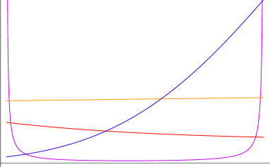
Figure 1: Behaviour of the scale factor (violet), internal scale factor (red), effective gravitational coupling (blue) and the string expansion parameter (yellow).

The case $\omega>-(d+1)/d$, implying $E<0$, which includes the pure string configuration, has been treated in reference [19], for an arbitrary dimension $D$. It is equivalent to changing the sign of the kinetic term for the field $\gamma$ in (5). The solution exhibits singularities, especially in the dilaton field: such singularity implies a breakdown of the string expansion, and the lagrangian (5) is not valid anymore.

3.3 Solutions with the moduli and axion fields, without the RR field

Let us now consider, besides the moduli fields, the axion field, that is $A\neq 0$, still in the absence of the RR field, that is, $\xi_{0}=0$. Equation (16) admits a simple solution if we choose a new time coordinate such that

$$dt=\tilde{E}\phi^{\frac{1+m}{2}}a^{3}d\vartheta\quad,\quad\tilde{E}=\frac{2}{1-m}\sqrt{\frac{3+2\omega}{2A^{2}}}\quad,$$ (38)

that is,

$$\phi=\phi_{0}\sin^{\frac{2}{1-m}}\vartheta\quad,\quad\phi_{0}=\biggr{\{}\frac{(3+2\omega)C}{2A^{2}}\biggl{\}}^{\frac{1}{1-m}}\quad,$$ (39)

$C$ being an integration constant. In terms of this new time parameter, and after the redefinition $a=\phi^{-1/2}b$, equation (15) takes the form, for the flat case,

$$\bigg{(}\frac{b^{\prime}}{b}\biggl{)}^{2}=\frac{3+2\omega}{3(1-m)^{2}}\biggr{\{}\frac{1}{\bar{C}}\biggr{[}{M}b^{2}-\frac{B^{2}}{6}\biggl{]}+1\biggl{\}}\frac{1}{\sin^{2}\vartheta}\quad,$$ (40)

where a prime means now derivative with respect to $\vartheta$, and

$$\bar{C}=\frac{3+2\omega}{12}C\quad\mbox{and}\quad{M}=\frac{8\pi G\rho_{0}}{3c^{2}}\quad,$$ (41)

leading to the relation

$$\int\frac{db}{b\sqrt{\tilde{M}b^{2}-N^{2}}}=\pm\frac{1}{1-m}\sqrt{\frac{3+2\omega}{3\bar{C}}}\ln\tan\frac{\vartheta}{2}\quad,$$ (42)

where $N^{2}=B^{2}/6-\bar{C}$. Notice that this excludes the case $\bar{C}>B^{2}/6$ since it would imply a non-regular solution, at least in the dilatonic field, as the final results indicate.

The result for the scale factor is:

$$a(\vartheta)=a_{0}\sin^{-1/(1-m)}\vartheta\frac{1}{\cos[pf(\vartheta)]}\quad;$$ (43)

where

$$\quad f(\vartheta)=\ln\tan\frac{\vartheta}{2}\ \quad,\quad p=\pm\frac{2}{1-m}\frac{N}{\sqrt{C}}\quad,$$ (44)

and

$$a_{0}=\biggl{(}\frac{6\bar{C}}{A^{2}}\biggr{)}^{1/[2(m-1)]}\frac{N}{\sqrt{\tilde{M}}}.$$ (45)

Moreover,

$$\Psi^{\prime} = \Psi_{0}\sin\xi\quad,$$ (46)

$$\gamma^{\prime} = \frac{\gamma_{0}}{\sin\vartheta}\quad,$$ (47)

where

$$\Psi_{0}=\frac{(3+2w)\sqrt{C}}{A(1-m)},$$ (48)

$$\gamma_{0}=\frac{2B}{(1-m)\sqrt{C}}.$$ (49)

The solutions found above describe a completely regular cosmological scenario. The scale factor behaves asymptotically as $a\propto|t|^{\frac{1}{2}}$ for $t\rightarrow\pm\infty$. The internal scale factor and the dilatonic field (consequently its inverse, the string perturbative parameter) $e^{-\sigma}$ are given by

$$e^{\beta}=\biggr{[}\tan\frac{\vartheta}{2}\biggl{]}^{\frac{\gamma_{0}}{r}}\phi(\vartheta)^{\frac{-s}{r}}\quad,$$ (50)

$$e^{-\sigma}=\biggr{[}\tan\frac{\vartheta}{2}\biggl{]}^{\frac{-d\gamma_{0}}{r}}\phi(\vartheta)^{\frac{r+ds}{r}}\quad.$$ (51)

The solution is completely regular in the sense that there is no curvature singularity. Also, the effective gravitational coupling $\phi$, the internal scale factor $e^{\beta}$ and the dilatonic field $e^{-\sigma}$ behave regularly. Moreover, the internal dimensions become small and stabilize for some choices of the integration parameters. The behaviour of these functions are similar to those displayed in figure $1$.

In order for having a bounce in the flat case in the Einstein frame, which is the case of the solutions presented above, the null energy condition $\rho+p>0$ must be violated near the bounce [20], being satisfied only far from the bounce. The fields which violate the null energy condition can be easily seen from the Lagrangians in the Einstein frame:

$$L=\sqrt{-g}\biggr{\{}R+\gamma_{;\rho}\gamma^{;\rho}-(\omega+3/2)\chi_{;\rho}\chi^{;\rho}-\exp(-2\chi)\Psi_{;\rho}\Psi^{;\rho}\biggl{\}}+L_{matter},$$ (52)

when the moduli field is present, and

$$L = \sqrt{-g}\biggr{\{}R+-(\omega+3/2)\chi_{;\rho}\chi^{;\rho}-\exp(-2\chi)\Psi_{;\rho}\Psi^{;\rho}-\exp(-\chi)\xi_{;\rho}\xi^{;\rho}\biggl{\}}$$ (53)

$$+ L_{matter}.$$

In the first case, the moduli field is the one which violates the null energy condition, while in the second case, if $\omega<-3/2$, is the dilaton which violate this condition: both have the “wrong” sign in their kinetic terms.

4 Spectrum of scalar perturbations

Before writing the perturbed equations, let us redefine the scalar fields as follows:

$$\chi = \ln\phi\quad,$$ (54)

$$\Psi = \zeta\quad.$$ (55)

All the fields are made a-dimensional. Hence, the field $\phi$ is redefined as [18]

$$\frac{3+2\omega}{4+2\omega}G\phi\quad\rightarrow\quad\phi\quad.$$ (57)

Moreover, the quantities with dimension of time or space are made dimensionless by using the Planck’s time ($t_{Pl}$) or length ($L_{Pl}$). The scale factor has no dimension. In what follows, the perturbative analysis will be performed in the Einstein frame, for technical simplicity. The final spectrum is computed in the Jordan frame.

The metric, including the background and the perturbed functions, has the form

$$ds^{2}=b^{2}(\eta)[(1+2\Phi)d\eta^{2}-(1-2\Psi)\gamma_{ij}dx^{i}dx^{j}]\quad,$$ (58)

where $\Phi=\Phi(\eta,\vec{x})$ and $\Psi=\Psi(\eta,\vec{x})$ are the metric fluctuations in the longitudinal gauge, $\eta$ is the conformal time, $dt=bd\eta$, and $b$ is the scale factor in the Einstein frame. We follow here the gauge invariant formalism [21]. We also define ${\cal{H}}=b_{\eta}/b$ (from now on, subscripts $\eta$ indicate derivatives with respect to the conformal time $\eta$). It is convenient to write separately the final perturbed equations for the case where the RR field is present and the moduli fields are absent and for the case where the RR field is absent and the moduli fields are present.

• Perturbed equations in the absence of the RR field:

  $$\Phi_{\eta\eta}+4{\cal{H}}\Phi_{\eta}-\biggr{\{}4k+\frac{\nabla^{2}}{3}\biggl{\}}\Phi=\frac{\bar{\omega}}{3}\chi_{\eta}\delta\chi_{\eta}$$

  $$+ \frac{m-1}{6}\zeta_{\eta}^{2}e^{(m-1)\chi}\delta\chi-\frac{\gamma_{\eta}}{3}\delta\gamma_{\eta}+\frac{\zeta_{\eta}}{3}e^{(m-1)\chi}\delta\zeta_{\eta}\quad,$$

  $$\delta\chi_{\eta\eta}+2{\cal{H}}\delta\chi_{\eta}-\biggr{\{}\nabla^{2}+\frac{(1-m)^{2}}{2\bar{\omega}}e^{(m-1)\chi}\zeta_{\eta}^{2}\biggl{\}}\delta\chi-4\chi_{\eta}\Phi_{\eta}$$

  $$+ \frac{(1-m)}{\bar{\omega}}e^{(m-1)\chi}\zeta_{\eta}\delta\zeta_{\eta}=0\quad,$$

  $$\delta\zeta_{\eta\eta}+[2{\cal{H}}+(m-1)\chi_{\eta}]\delta\zeta_{\eta}-\nabla^{2}\delta\zeta-4\Phi_{\eta}\zeta_{\eta}$$

  $$+ (m-1)\zeta_{\eta}\delta\chi_{\eta}=0\quad,$$ (62)

  $$\delta\gamma_{\eta\eta}+2{\cal{H}}\delta\gamma_{\eta}-\nabla^{2}\delta\gamma-4\Phi_{\eta}\gamma_{\eta}=0\quad,$$

  where

  $$\bar{\omega}=3/2+\omega\quad.$$ (63)

• Perturbed equations in the absence of the moduli fields ($m=-1$):

  $$\Phi_{\eta\eta}+4{\cal{H}}\Phi_{\eta}-\biggr{\{}4k+\frac{\nabla^{2}}{3}\biggl{\}}\Phi=\frac{\bar{\omega}}{3}\chi_{\eta}\delta\chi_{\eta}$$

  $$+\frac{e^{-2\chi}}{3}\zeta_{\eta}\delta\zeta_{\eta}-\biggr{[}\frac{e^{-2\chi}}{3}\zeta_{\eta}^{2}+\frac{e^{-\chi}}{12}\xi_{\eta}^{2}\biggl{]}\delta\chi+\frac{e^{-\chi}}{6}\xi_{\eta}\delta\xi_{\eta} \quad,$$ (64)

  $$\delta\chi_{\eta\eta}+2{\cal{H}}\delta\chi_{\eta}-\biggr{\{}\nabla^{2}+\frac{1}{4\bar{\omega}}e^{-\chi}\xi_{\eta}^{2}+\frac{2}{\bar{\omega}}e^{-2\chi}\zeta_{\eta}^{2}\biggl{\}}\delta\chi$$

  $$-4\chi_{\eta}\Phi_{\eta}+\frac{2}{\bar{\omega}}e^{-2\chi}\zeta_{\eta}\delta\zeta_{\eta}+\frac{1}{2\bar{\omega}}e^{-\chi}\xi_{\eta}\delta\xi_{\eta} = 0\quad,$$ (65)

  $$\delta\zeta_{\eta\eta}+2({\cal{H}}-\chi_{\eta})\delta\zeta_{\eta}-\nabla^{2}\delta\zeta-4\Phi_{\eta}\zeta_{\eta}-2\zeta_{\eta}\delta\chi_{\eta} = 0\quad,$$ (67)

  $$\delta\xi_{\eta\eta}+(2{\cal{H}}-\chi_{\eta})\delta\xi_{\eta}-\nabla^{2}\delta\xi-4\Phi_{\eta}\xi_{\eta}-\xi_{\eta}\delta\chi_{\eta} = 0\quad,$$ (68)

  where now

  $$\bar{\omega}=3/2+\tilde{\omega}\quad.$$ (69)

In equations (• ‣ 4-62) and (• ‣ 4-68) the perturbed variables are $\Phi$, $\delta\chi$, $\delta\zeta$, $\delta\gamma$ and $\delta\xi$, and the background quantities are ${\cal{H}}$, $\chi$, $\gamma$, $\zeta$ and $\xi$.

Equations (• ‣ 4-62) and (• ‣ 4-68) are written using the conformal time. The background solutions are expressed in terms of the time parameter $\tau$ (for $m=-1$) or $\vartheta$ (for $m\neq-1$). If we consider the perturbed equations (• ‣ 4-68), for example, and changing to the time parameter $\tau$, we obtain,

$$\Phi^{\prime\prime}+(2h+\chi^{\prime})\Phi^{\prime}-\biggr{\{}4k+\frac{\nabla^{2}}{3}\biggl{\}}e^{-2\chi}b^{4}\Phi=\frac{\bar{\omega}}{3}\chi^{\prime}\delta\chi^{\prime}$$

$$+\frac{e^{-2\chi}}{3}\zeta^{\prime}\delta\zeta^{\prime}-\biggr{[}\frac{e^{-2\chi}}{3}\zeta^{\prime 2}+\frac{e^{-\chi}}{12}\xi^{\prime 2}\biggl{]}\delta\chi+\frac{e^{-\chi}}{6}\xi^{\prime}\delta\xi^{\prime} \quad,$$ (70)

$$\delta\chi^{\prime\prime}+\chi^{\prime}\delta\chi^{\prime}-\biggr{\{}e^{-2\chi}b^{4}\nabla^{2}+\frac{1}{4\bar{\omega}}e^{-\chi}\xi^{\prime 2}+\frac{2}{\bar{\omega}}e^{-2\chi}\zeta^{\prime 2}\biggl{\}}\delta\chi$$

$$-4\chi^{\prime}\Phi^{\prime}+\frac{2}{\bar{\omega}}e^{-2\chi}\zeta^{\prime}\delta\zeta^{\prime}+\frac{1}{2\bar{\omega}}e^{-\chi}\xi^{\prime}\delta\xi^{\prime} = 0\quad,$$ (71)

$$\delta\zeta^{\prime\prime}-\chi^{\prime}\delta\zeta^{\prime}-e^{-2\chi}b^{4}\nabla^{2}\delta\zeta-4\Phi^{\prime}\zeta^{\prime}-2\zeta^{\prime}\delta\chi^{\prime} = 0\quad,$$ (72)

$$\delta\xi^{\prime\prime}-e^{-2\chi}b^{4}\nabla^{2}\delta\xi-4\Phi^{\prime}\xi^{\prime}-\xi^{\prime}\delta\chi^{\prime} = 0\quad,$$ (73)

where $h=b^{\prime}/b$. These are the equations which will be integrated numerically. The other cases follow the same lines.

The operator $\nabla^{2}$ acts on the three-dimensional section at constant curvature, and its eigenfunctions are plane waves ($k=0$), spherical harmonics ($k=1$) and pseudo-spherical harmonics ($k=-1$). From now on, we will restrict ourselves to the flat case. Hence, the perturbed quantities, represented generically by $\delta_{n}$, can be decomposed into Fourier components:

$$\delta(\eta,\vec{x})=\frac{1}{(2\pi)^{3/2}}\int\delta_{n}(\eta,\vec{n})e^{i\vec{n}.\vec{x}}d^{3}n\quad,$$ (74)

where the Fourier components $\delta_{k}$ obey the Helmholtz equation

$$\nabla^{2}\delta_{n}=-n^{2}\delta_{n}\quad.$$ (75)

We are adopting the convention that the coordinates have dimensions of length while the metric is dimensionless. Hence the wave number has dimensions of ${\rm cm}^{-1}$. The range of interest for the wavenumber $\vec{n}$ corresponds to scales where the approximation of isotropy and homogeneity is valid. Today, these scales are roughly between $100\,Mpc$ and $3.000\,Mpc$. In order to fix the initial interval of $\vec{n}$ corresponding to those scales today, we match asymptotically the solutions found with the standard cosmological phase. This task becomes easier since the asymptotic behaviour of the solutions presented here coincides with the radiative phase of the standard cosmological model. If $\tau_{f}$ ($\vartheta_{f}$) corresponds to the final asymptote of the solutions, we fix this matching at $\tau_{m}$ ($\vartheta_{m}$) such that

$$\frac{\tau_{f}-\tau_{m}}{\tau_{m}}=10^{-5}\quad.$$ (76)

The choice of the precision of the matching does not affect essentially the final results unless it is too small, so that numerical computation may become doubtful.

From $\tau=\tau_{m}$ ($\vartheta=\vartheta_{m}$) on the Universe follows the evolution dictated by the standard cosmological model. We generally impose that this happens before the nucleosynthesis period. Hence, imposing that the scale factor today equals unity (such that today the physical scales correspond to the coordinate scales), this normalization implies that the matching must occur when $a<10^{-12}$. Consider, for example, that the matching is made exactly at $a=10^{-12}$, and that at this moment the gravitational coupling is constant, so that the formulation in the Einstein frame becomes identical to that of the Jordan frame, $a=b$.

To be specific, let us take the pure anomalous axionic solution of subsection (3.1) as an example (the other solutions follow the same lines), with $\omega=-3$. We define the dimensioless parameter $\theta=\alpha\tau$ with range $2{\rm arctgh}\exp(-7\pi/2)<\theta<2{\rm arctgh}\exp(-3\pi/2)$. In $\theta_{m}$ we have

$$b(\theta_{m}) = b_{0}\biggr{[}1-\sin f(\theta)\biggl{]}^{-1/2}=10^{-12}\quad,$$ (77)

$$\phi(\theta_{m}) = \phi_{0}\sinh(\theta_{m})=1\quad,$$ (78)

remembering that, for this $\omega$,

$$f(\theta)=\ln\biggr{[}\biggr{|}\tanh\biggr{(}\frac{\theta}{2}\biggl{)}\biggl{|}\biggl{]}.$$ (79)

These relations lead to $b_{0}=10^{-18}$ and $\phi_{0}=\sinh(3\pi/2)$. Using Eqs (• ‣ 3.1), we obtain

$$\alpha=A\sqrt{\frac{2}{3}}=10^{-50}{\rm cm}^{-1},\quad,\quad p=1\quad{\rm and}\quad M=10^{-60}{\rm cm}^{-2}.$$ (80)

Equations (4–73) then reads

$$\Phi_{\theta\theta}+\biggl{\{}\frac{\cos f(\theta)}{[1-\sin f(\theta)]\sinh(\theta)}+{\rm cotgh}(\theta)\biggr{\}}\Phi_{\theta}$$

$$+ \frac{{\tilde{n}}^{2}}{3\sinh^{2}(\theta)[1-\sin f(\theta)]^{2}\sinh^{2}(3\pi/2)}\Phi$$

$$= -{\rm cotgh}(\theta)\delta\chi_{\theta}+\frac{\delta\zeta_{\theta}}{\sqrt{6}\sinh(3\pi/2)\sinh(\theta)}-\frac{3}{2}\delta\chi\quad,$$

$$\delta\chi_{\theta\theta}+{\rm cotgh}(\theta)\delta\chi_{\theta}+\biggr{\{}\frac{{\tilde{n}}^{2}}{\sinh^{2}(\theta)[1-\sin f(\theta)]^{2}\sinh^{2}(3\pi/2)}-1\biggl{\}}\delta\chi$$

$$= 4{\rm cotgh}(\theta)\Phi_{\theta}+\frac{\sqrt{2}}{\sqrt{3}\sinh(3\pi/2)\sinh(\theta)}\delta\zeta_{\theta}\quad,$$

$$\delta\zeta_{\theta\theta}-{\rm cotgh}(\theta)\delta\zeta_{\theta}+\frac{{\tilde{n}}^{2}}{\sinh^{2}(\theta)[1-\sin f(\theta)]^{2}\sinh^{2}(3\pi/2)}\delta\zeta$$

$$= 2\sqrt{6}\sinh(3\pi/2)\sinh(\theta)\Phi_{\theta}+\sqrt{6}\sinh(3\pi/2)\sinh(\theta)\delta\chi_{\theta}\quad.$$ (83)

In these equations $\tilde{n}\equiv nb_{0}^{2}/\alpha$.

The final step is to fix the initial conditions. The most natural way is to impose that the initial spectrum is determined by quantum fluctuations. The determination of this spectrum follows the standard procedure[21, 22]. First of all we must remark that the perturbed functions decouple for $\eta\rightarrow-\infty$. Hence, all perturbed quantities behave as free fields. The metric fluctuation must be expressed in terms of a new variable that is formally equivalent to a free scalar field. At this moment, the fields are quantized, leading to normalized modes. Choosing an initial vacuum state, the initial spectrum expressed in the conformal time reads

$$\Phi_{n}\propto 3\sqrt{\frac{3}{2}}\frac{\beta}{{\cal{H}}n^{2}}\biggr{(}\frac{v_{n}}{z}\biggl{)}_{\eta}\quad,$$ (84)

$$v_{n}=\frac{1}{\sqrt{2c_{s}n}}e^{-ic_{s}n\eta}\quad,$$ (85)

where $\beta={\cal{H}}^{2}-{\cal{H}}^{\prime}$, $z=\frac{b\beta^{1/2}}{c_{s}H}$ and $c_{s}=1/\sqrt{3}$. For the other fields, represented generically by $u$, one has

$$u_{n}\propto\frac{1}{\sqrt{2n}}e^{-in\eta}\quad.$$ (86)

In terms of the $\theta$ parameter one has:

$$\Phi_{n}^{\rm ini} \propto \frac{3^{3/4}\sinh^{3}(7\pi/2)(\theta-\theta_{i})^{2}}{8b_{0}^{3}{\tilde{n}}^{3/2}}\biggl{[}\frac{\sqrt{3}(\theta_{i}-\theta)\sinh^{2}(7\pi/2)}{4\tilde{n}b_{0}^{2}}+i\biggr{]}$$ (87)

$$\times \exp\biggl{[}\frac{i\tilde{n}4b_{0}^{2}}{\sqrt{3}\sinh^{2}(7\pi/2)(\theta-\theta_{i})}\biggr{]}$$

and

$$\delta\chi_{k}^{\rm ini}\propto\frac{\sinh(7\pi/2)(\theta-\theta_{i})}{2b_{0}{\tilde{n}}^{1/2}}\exp\biggl{[}\frac{i\tilde{n}4b_{0}^{2}}{\sinh^{2}(7\pi/2)(\theta-\theta_{i})}\biggr{]}.$$ (88)

With these initial conditions, the system is left to evolve. Due to the complexity of the perturbed equations and of the background solutions, the system of equations is solved numerically, with the initial conditions fixed as described before, using the software Mathematica. The processed final spectrum is given by

$$P_{n}={\bar{\Phi}}_{n}^{2}\,n^{3}\propto n^{n_{s}}\quad,$$ (89)

where $n_{s}$ is the spectral index. The Bardeen potential $\bar{\Phi}$ in the Jordan frame is related to the potential in the Einstein frame by

$$\bar{\Phi}=\Phi+\frac{\delta\chi}{2}\quad.$$ (90)

The spectrum is computed at the moment the universe matches the standard model in the radiative era before the nucleosynthesis. The general behaviour of the spectrum, for all cases, is given in figure $1$ for a large range of values of $n$. In general, it display an oscillating behaviour with decreasing amplitude. However, the cosmological scales of interest, determined by the matching conditions together with the normalization of the scale factor today, imply $n<<1$. For this case, and for scales today between $100\,Mpc$ and $3.000\,Mpc$ the spectrum has the shape displayed in figure $2$, again for all the cases treated in the present study. It is a decreasing spectrum, in strong disagreement with the observation which indicates a nearly Harrisson-Zeldovich spectrum [23]. It is remarkable that in all different cases the spectral index is essentially $n=-2$. We have computed the spectrum at constant time and, in this situation, a Harrison-Zeldovich spectrum implies that $P_{n}$ grows with $n$.

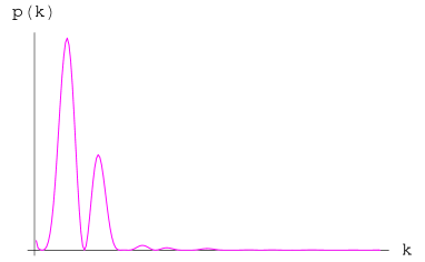
Figure 2: General form of the spectrum.

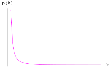
Figure 3: The predicted spectrum for scales up to the Hubble radius.

5 Conclusions

We have studied cosmological models based on the string effective action at tree level. The dilaton, the axion, RR and the moduli fields were taken into account, besides gauge fields coming from the Ramond-Ramond sector. Two free parameters were introduced in the effective lagrangian, $\omega$ and $m$, connected with the coupling of the dilaton and axion fields. These parameters were kept free in order to cover fundamental theories, like $M$ and $F$ theories, as well as $p$-branes configurations in the superstring theory. Regular solutions were found, but only for cases where $\omega<-1$, which excludes the pure string case. The new solutions found here, taking into account the moduli fields, exhibit compactification of the extra dimensions. The scale factor displays a bounce, exhibiting initially a contracting phase before entering the expansion phase. Asymptotically, a radiative phase is recovered allowing to match the solution with the standard cosmological model. At the same time, the string expansion parameter remains finite during the whole evolution of the universe. The effective gravitational coupling decreases with time what, at least, alleviate the hierarchial problem related to the characteristic energy scale of gravity.

The properties of the solutions found reveal that such ”string” cosmological models can be candidates for describing the primordial phase of the universe. However, traces from this primordial phase can be compared with observations through the evaluation of the power spectrum of scalar fluctuations. This primordial power spectrum is inferred from the spectrum of the anisotropy of the CMBR. The observational results favor a flat spectrum. Here, we have computed the spectrum at the beginning of the radiative phase supposing that the initial fluctuations were formed in the beginning of the contraction phase, before the bounce, and that they were of quantum mechanical origin. The quantum fluctuations are compatible with the asymptotical behaviour in the beginning of the contracting phase. However, the final spectrum is strongly decreasing, in contradiction with the observational results, which favors at least a quasi-scale invariant spectrum. Hence, the regular solutions found, in spite of their nice features, are not candidate for a realistic primordial cosmological model, The same features are found for the regular ”anomalous” solutions found in reference [15].

In fact, the result $n_{s}=-2$ for the spectral index is not surprising. In reference [22], the same spectrum has been obtained in the Einstein frame for a scalar field with negative kinetic energy together with radiation. Here the situation is very similar, see equations (52,53), but with the presence of other fields. These other fields do not alter the bounce itself and, most important, the asymptotic behaviour. It seems that the intermediate phase they can be important is not relevant for the spectrum at large scales. Going to the Jordan’s frame does not modify the result because the spectrum of $\delta\chi$ is negligible with respect to that of $\Phi$ for small wave numbers.

These results seem to exclude such string motivated models at tree level. Nevertheless, it must be stressed that in the model developed here a quite simple compactification mechanism was considered: the internal space is flat, a $d$-dimensional torus. String theory admits many other kinds of compactifications. In particular, the Calabi-Yau manifolds are especially interesting since they can accommodate, in quite natural way, the gauge groups of the standard model of particle physics [8]. In this case, the effective model in four dimensions will be different to the one we have studied here. However, the negative results reported here indicate difficulties in constructing meaningful realistic cosmological models based on string motivated effective actions at tree level.

Acknowledgments: We thank CNPq (Brazil) and CAPES (Brazil) for partial financial support. We thank also Jérôme Martin and Patrick Peter for their criticisms and suggestions.

References

- [1] E.W. Kolb and M.S. Turner, The early universe, Addison-Wesley, New York(1990);
- [2] J. Garcia-Bellido, Cosmology and astrophysics, astro-ph/0502139;
- [3] D.H. Lyth and A. Riotto, Phys. Rep. 314, 1(1999);
- [4] D.J. Schwarz, C.A. Terrero-Escalante, JCAP 0408, 03(2004);
- [5] W.H. Kinney, Inflation after WMAP, astro-ph/0406670;
- [6] A. Lue, G.D. Starkman, T. Vachaspati, A post-WMAP perspective on inflation, astro-ph/0303268;
- [7] J. Polchinski, String theory, volumes I and II, Cambridge University Press, Cambridge(1998);
- [8] M. B. Green, J.H. Schwarz, and E. Witten, Superstring theory, Cambridge University Press, Cambridge(1987);
- [9] E. Kiritsis, Introduction to superstring theory, hep-th/9709062;
- [10] J.E. Lidsey, D. Wands, and E.J. Copeland, Phys. Rep. 337, 343 (2000);
- [11] M. Gasperini and G. Veneziano, The pre-big bang scenario in string cosmology, hep-th/0207130;
- [12] J. Khoury, B. A. Ovrut, P. J. Steinhardt, and N. Turok, Phys. Rev. D64, 123522 (2001); hep-th/0105212; R. Y. Donagi, J. Khoury, B. A. Ovrut, P. J. Steinhardt, and N. Turok, JHEP 0111, 041 (2001).
- [13] S.P. Patil, R.H. Brandenberger, The cosmology of massless string modes, hep-th/0502069;
- [14] C.P. Constantinidis, J.C. Fabris, R.G. Furtado, and M. Picco, Phys. Rev. D61, 043503 (2000);
- [15] J.C. Fabris, R.G. Furtado, P. Peter and N. Pinto-Neto, Phys. Rev. D67, 124003(2003);
- [16] K.A. Bronnikov and J.C. Fabris, JHEP 209, 62 (2002);
- [17] M. Tegmark et al, Phys. Rev. D69, 103501(2004);
- [18] S. Weinberg, Gravitation and cosmology, Wiley, New York(1972);
- [19] S. Tsujikawa, Class. Quant. Grav. 20, 1991(2003);
- [20] P. Peter and N. Pinto-Neto, Phys.Rev. D65 023513 (2002);
- [21] V.F. Mukhanov, H.A. Feldman and R.H. Brandenberger, Phys. Rep. 215, 203(1992);
- [22] P. Peter and N. Pinto-Neto, Phys. Rev. D66, 063509(2002);
- [23] C.L. Bennet et al, Astrophys. J. Suppl. 148, 1(2003).