Observation of String Breaking in QCD

Abstract

We numerically investigate the transition of the static quark-antiquark string into a static-light meson-antimeson system. Improving noise reduction techniques, we are able to resolve the signature of string breaking dynamics for $n_{f}=2$ lattice QCD at zero temperature. This result can be related to properties of quarkonium systems. We also study short-distance interactions between two static-light mesons.

I Introduction

Sea quarks are an important ingredient of strong interaction dynamics. In the framework of quantum chromodynamics, however, quantitative calculations of their effects on hadron phenomenology have proven to be notoriously difficult, unless one resorts to approximations based on additional model assumptions. Nevertheless, the ab initio approach of lattice gauge theory towards the sea quark problem has shown steady progress over the past decade: recently the $\eta^{\prime}$-problem has been tackled successfully on the lattice Schilling:2004kg ; Struckmann:2000bt ; McNeile:2001cr where sea quarks induce the axial anomaly in the sense of the Witten-Veneziano mechanism Witten:1979vv ; Veneziano:1980xs .

Another example is the strong decay of hadrons through light quark-antiquark pair creation, for instance the transition from a colour string configuration between two static colour sources, $\overline{Q}Q$, into a pair of static-light mesons, $B\overline{B}$. This colour string breaking, which we address in this paper, is expected to occur as soon as the colour source-sink separation, $r$, exceeds a certain threshold value, $r_{c}>1\,\mbox{fm}$.

In lattice simulations this behaviour has been investigated in four dimensional QCD at zero temperature $T$ with sea quarks Bali:2000vr ; bolder ; Aoki:1998sb ; Bonnet:1999gt ; Pennanen:2000yk ; Duncan:2000kr ; Bernard:2001tz as well as in QCD₃ Trottier:2004qc . However, these studies lacked compelling evidence of string breaking. This failure is due to problems like: (i) String breaking investigations only make sense in a full QCD setting with large ensemble sizes. (ii) String breaking occurs at distances beyond 1 fm, a regime with a poor signal-to-noise ratio. (iii) The poor overlap of the $\overline{Q}Q$ creation operator with the large-distance $B\overline{B}$ ground state.

This last problem necessitates to resolve the signal at huge Euclidean times $t$, unless one bases the investigation on a $2\times 2$ correlation matrix, whose additional elements include the insertion of light quark propagators into the standard Wilson loop Pennanen:2000yk ; Duncan:2000kr ; Bernard:2001tz ; bolder . Such quark insertions require propagators from any source to any sink position (“all-to-all propagators”), in order to enable the exploitation of translational invariance for error reduction (self averaging).

For QCD with $n_{f}$ mass-degenerate sea quark flavours this correlation matrix takes the form,

$$C(t)\quad= \left(\begin{array}[]{cc}C_{QQ}(t)&C_{QB}(t)\\ C_{BQ}(t)&C_{BB}(t)\end{array}\right)$$ (3)

$$=e^{-2m_{Q}t}\!\!\!\!\! \left(\begin{array}[]{rl}\quad\mbox{ \begin{minipage}{16.0pt}\includegraphics[width=16.0pt]{w11.ps}\end{minipage}}&\quad\sqrt{n_{f}}\mbox{ \begin{minipage}{16.0pt}\includegraphics[width=16.0pt]{w12.ps}\end{minipage}}\\ &\\ \sqrt{n_{f}}\mbox{ \begin{minipage}{16.0pt}\includegraphics[width=16.0pt]{w21.ps}\end{minipage}}&\quad-n_{f}\mbox{ \begin{minipage}{16.0pt}\includegraphics[width=16.0pt]{w22c.ps}\end{minipage}}+\mbox{ \begin{minipage}{16.0pt}\includegraphics[width=16.0pt]{w22d.ps}\end{minipage}}\end{array}\right),$$ (7)

where the straight lines denote gauge transporters and the wiggly lines represent light quark propagators. We refer to the difference between the physical eigenstates and the $\overline{Q}Q$ and $B\overline{B}$ basis as “mixing”. Such mixing should manifest itself “explicitly”, by non-vanishing off-diagonal matrix elements, relative to the diagonal matrix elements, and “implicitly”. The latter refers either to the Wilson loop $C_{QQ}(t)$ decaying into the mass of the (dominantly) $B\overline{B}$ state for $r>r_{c}$ or to a decay of $C_{BB}(t)$ towards the $\overline{Q}Q$ mass for $r<r_{c}$, as $t\rightarrow\infty$. Implicit mixing is much harder to detect than explicit mixing.

In the quenched approximation baryon and anti-baryon numbers are separately conserved and the $\overline{Q}Q$ and $B\overline{B}$ sectors are mutually orthogonal. By definition, $n_{f}$ vanishes and there will be no mixing. This does not mean however, that the matrix elements accompanying the explicit $n_{f}$- and $\sqrt{n_{f}}$-factors are necessarily zero.

So far string breaking has been verified in the following cases: in $SU(2)$ gauge theory with a fundamental scalar field in three dimensions Philipsen:1998de and in four dimensions Jersak:1988bf ; Bock:1988kq ; Knechtli:1998gf as well as for the $SU(2)$ potential between adjoint sources (screened by the gluons) in three dimensions Poulis:1995nn ; Stephenson:1999kh ; Philipsen:1999wf ; Kratochvila:2003zj and in four dimensions deForcrand:1999kr ; Kallio:2000jc . However, in only one of these studies Kratochvila:2003zj , and in a recent simulation of the 3d ${\mathbb{Z}}_{2}$-Higgs model Gliozzi:2004cs , implicit string breaking has been convincingly demonstrated.

Let us recall the signature of string breaking: without mixing, the $\overline{Q}Q$ and the $B\overline{B}$ are QCD eigenstates and will undergo a plain level crossing (with minimal energy gap $\Delta E_{c}=0$), at a certain critical distance $r_{c}$. Simulations with $n_{f}=0$ show exactly this behaviour. In contrast, with $q\bar{q}$ creation/annihilation switched on, the Fock states will undergo sizeable mixing in the neighbourhood of $r_{c}$. The minimal energy gap $\Delta E_{c}$ between the two eigenstates will grow with the spatial width of the mixing region.

The transition rate between $\overline{Q}Q$ and $B\overline{B}$ states is given by the (normalized) time derivative of the off-diagonal matrix element, $g=[dC_{QB}(t)/dt]_{t=0}[C_{BB}(0)C_{QQ}(0)]^{-1/2}$. From a string picture as well as from strong coupling arguments one would expect a more pronounced mixing in larger space-time dimensions $d$. Therefore, the size of the energy gap within the string breaking region should increase as one goes from $d=3$ to $d=4$. In the large $N_{c}$ limit we find, $g\propto\sqrt{n_{f}/N_{c}}$, for the potential between fundamental sources, screened by $n_{f}$ flavours of fundamental scalar or quark fields. For the breaking of the adjoint potential this translates into, $g\propto 1/N_{c}$.

The figures of Refs. Philipsen:1999wf ; Stephenson:1999kh for the adjoint string in 3d $SU(2)$ gauge theory suggest the following upper limits for the size of the energy gap, expressed in units of the string breaking distance: $\Delta E_{c}r_{c}<0.45$ and $\Delta E_{c}r_{c}<0.75$, respectively. In 4d $SU(2)$ gauge theory one finds, $\Delta E_{c}r_{c}<0.6$ deForcrand:1999kr , whereas Refs. Philipsen:1998de ; Knechtli:1998gf show that the fundamental 3d $SU(2)$ string, screened by a scalar field, satisfies $\Delta E_{c}r_{c}<0.35$ and $\Delta E_{c}r_{c}<0.65$, respectively. In all these cases either the spatial resolution of the string breaking region was too coarse or the statistical errors were too large to allow for the determination of a lower bound.

Based on the qualitative $n_{f}$, $N_{c}$ and $d$-dependencies discussed above, we expect the $n_{f}=2$ QCD energy gap to be somewhat bigger than the gaps quoted for the toy model studies. From this reasoning we would aim at an error of $\Delta E_{c}r_{c}$, smaller than 0.1. To meet this constraint, we require a distance resolution in the string breaking region of $\Delta r<0.1/(\sigma r_{c})\approx 0.02\,r_{c}\approx 0.025$ fm, where $\sigma$ denotes the string tension. We will find, $\Delta E_{c}r_{c}=0.33(5)$.

In order to achieve the required precision, we apply a fourfold arsenal of critical improvements, within the $2\times 2$ correlation matrix setting:

Ground state overlaps.

It is essential to achieve a large overlap between the trial wavefunctions and the respective physical ground states. This enhances the signal since it will decay less rapidly with Euclidean time. Moreover, the large $t$ asymptotics will be reached at smaller temporal distances, further reducing the noise/signal ratio. To this end we employ combinations of APE and Wuppertal smearing techniques (see Sec. III.2).

Wilson loops.

The Wilson loop signal $C_{QQ}(t)$ can be further enhanced by using an improved fat link static action. In this way, the relative errors of the Wilson loop data are reduced by factors of about five (see Sec. III.2).

Quark propagators.

The generalized Wilson loops of Eq. (7) require the computation of all-to-all light quark propagators if we wish to fully exploit self averaging. Direct inversion of the Wilson Dirac matrix $M$ would be computationally prohibitive. Therefore, we approximate $M^{-1}$ by the lowest lying eigenvectors of $\gamma_{5}M$ using the truncated eigenmode approach (TEA) Neff:2001zr , together with a stochastic estimation (SET, see e.g. the review Wilcox:1999ab ) in the orthogonal subspace. Moreover, we apply a “hopping parameter acceleration” (HPA) for variance reduction. This further reduces the errors of the disconnected contribution to $C_{BB}$ by factors of about three (see Sec. III.3).

Distance resolution.

In order to avoid finite size effects and to achieve a fine distance resolution of the string breaking region, we employ a large set of off-axis distances (see Sec. III.1).

With these methods we are able to demonstrate compelling evidence, both for explicit mixing and for string breaking in full QCD, as well as for implicit mixing within $C_{BB}(t)$ for $r<r_{c}$. We find the breaking of the quark antiquark string to occur at a distance $r_{c}\approx 15\,a\approx 2.5\,r_{0}\approx 1.25$ fm, in units of $r_{0}\approx 0.5$ fm Sommer:1993ce ; Bali:1998pi .

Note that our study should be viewed as exploratory since we restrict ourselves to one value of the sea quark mass (slightly below the physical strange quark mass), at one lattice spacing. For details on our simulation parameters, see Sec. III.1.

The paper is organized as follows: in Sec. II we discuss the mixing problem in detail. The notation used within Eq. (7) will be defined. We describe the combined application of TEA, SET and HPA for the calculation of all-to-all propagators in Sec. III. In Sec. IV we discuss theoretical expectations for the individual matrix elements and check these against our data. In Sec. V, we present and interpret our main result, string breaking in QCD, as well as the short-distance interactions between two static-light mesons with isospin $I=0$ and $I=1$. We comment on the phenomenological implications in Sec. VI.

In view of the length of this paper, we kept the sections as self-contained as possible. For instance, the reader who is less interested in the technical aspects of the study can safely skip Sec. III altogether and concentrate on Secs. V and VI.

II The mixing problem

Let us consider a system with a heavy quark $Q$ and a heavy antiquark $\overline{Q}$ in the static approximation, with separation $r=|{\mathbf{R}}|/a$, where $a$ denotes the lattice spacing and ${\mathbf{R}}$ is an integer valued three-vector. We restrict our discussion to the $\Sigma_{g}^{+}$ ground state of the static system, with cylindrical symmetry.

Without sea quarks, the energy of this static-static system will linearly diverge with $r$ Bali:1992ru ; Booth:1992bm ; Bali:2000gf as $r\rightarrow\infty$. In the presence of sea quarks, however, there will be some critical “string breaking” distance $r_{c}$: when $r$ exceeds $r_{c}$, the mass of a system containing two static-light mesons, which we shall call $B$ and $\overline{B}$, separated by $r$, will become energetically favoured. The static $\overline{Q}Q$ potential will exhibit screening and saturate towards about twice the mass of the $B$ meson.

A full investigation of this phenomenon requires the study of the Green functions that correspond to the propagation of the $\overline{Q}Q$ and $B\overline{B}$ systems as well as of the transition element between these two states. We start by defining our notations and discussing the symmetries of the problem, before we display the relevant Green functions.

II.1 Definitions and representations

The Euclidean Dirac equation in the static limit,

$$\left(D_{4}\gamma_{4}+m_{Q}\right)|Q\rangle=0,$$ (8)

yields the propagators of static quark and antiquark:

$$Q_{y}\overline{Q}_{x} = \langle y|Q\rangle\langle Q|\gamma_{4}|x\rangle$$

$$= \delta_{{\mathbf{x}}{\mathbf{y}}}U_{{\mathbf{x}}}(y_{4},x_{4})e^{-m_{Q}(y_{4}-x_{4})}P_{+},$$

$$\overline{Q}^{\dagger}_{y}Q^{\dagger}_{x} = \langle y|\overline{Q}\rangle\langle\overline{Q}|\gamma_{4}|x\rangle$$

$$= \delta_{{\mathbf{x}}{\mathbf{y}}}U^{\dagger}_{{\mathbf{x}}}(y_{4},x_{4})e^{-m_{Q}(y_{4}-x_{4})}P_{-},$$

where $y_{4}\geq x_{4}$ and,

$$P_{\pm}=\frac{1\pm\gamma_{4}}{2},$$ (11)

are projectors onto the upper and lower two Dirac components. $U_{{\mathbf{x}}}(y_{4},x_{4})\in SU(3)$ denotes a lattice discretization of the Schwinger line, connecting $({\mathbf{x}},x_{4})$ with $({\mathbf{x}},y_{4})$:

$$U_{{\mathbf{x}}}(y_{4},x_{4})\simeq T\,\exp\left\{ig\int_{x_{4}}^{y_{4}}\!\!\!\!dt\,A_{4}({\mathbf{x}},t)\right\}.$$ (12)

$T$ denotes the time ordering operator. We use the convention $\langle x|Q\rangle=Q_{x}$ and $\langle Q|x\rangle=Q^{\dagger}_{x}$, i.e.  $\overline{Q}_{x}=\langle Q|\gamma_{4}|x\rangle$.

$m_{Q}(a)$ in Eqs. (II.1) and (II.1) above is the heavy quark mass in a lattice scheme. We define the light quark Dirac operator,

$$M=\left(|q\rangle\langle q|\gamma_{4}\right)^{-1}=D_{\mu}\gamma_{\mu}+m.$$ (13)

We use Wilson fermions throughout the paper:

$$M_{xy}=\delta_{xy}-\kappa\sum_{\mu=1}^{4} \left[(1-\gamma_{\mu})U_{x,\mu}\delta_{x+a\hat{\mu},y}\right.$$ (14)

$$+\left.(1+\gamma_{\mu})U_{x,-\mu}\delta_{x-a\hat{\mu},y}\right].$$

As usual, the quark fields have been rescaled by factors $\sqrt{2\kappa}$ where $\kappa=(8+2ma)^{-1}$ in the free field case and in general, $\kappa(m=0)=\kappa_{c}\geq 1/8$. $U_{x,\mu}$ denotes an $SU(3)$ gauge field and $U_{x,-\mu}=U^{\dagger}_{x-a\hat{\mu},\mu}$, $M^{\dagger}=\gamma_{5}M\gamma_{5}$.

We define a gauge transporter $V_{t}({\mathbf{y}},{\mathbf{x}})\in SU(3)$, connecting the point $({\mathbf{x}},t)$ with $({\mathbf{y}},t)$. This is to be taken local in time and rotationally symmetric about the shortest connection. The properties under local gauge transformations $\Omega_{x}\in SU(3)$ are:

$$Q_{x}\mapsto\Omega_{x}Q_{x},\quad\overline{Q}_{x}\mapsto\overline{Q}_{x}\Omega_{x}^{\dagger},$$ (15)

$$V_{t}({\mathbf{y}},{\mathbf{x}})\mapsto\Omega_{({\mathbf{y}},t)}V_{t}({\mathbf{y}},{\mathbf{x}})\Omega^{\dagger}_{({\mathbf{x}},t)},$$ (16)

which implies that the combination,

$${\mathcal{Q}}_{t}({\mathbf{y}},{\mathbf{x}})=\overline{Q}_{({\mathbf{y}},t)}\frac{\boldsymbol{\gamma}\cdot\mathbf{r}}{r}V_{t}({\mathbf{y}},{\mathbf{x}})Q_{({\mathbf{x}},t)},$$ (17)

is a colour singlet.

The spins of $\overline{Q}$ and $Q$ can either couple symmetrically or anti-symmetrically. The first situation is represented by ${\boldsymbol{\gamma}\cdot\mathbf{r}}/{r}$ in Eq. (17) (total spin $S=1$), the latter choice corresponds to the replacement, $\boldsymbol{\gamma}\cdot{\mathbf{r}}/r\mapsto\gamma_{5}$, within Eq. (17) ($S=0$), see also Ref. Drummond:1998ir .

The relevant symmetry group is not $O(3)\otimes{\mathcal{C}}$ but its cylindrical subgroup $D_{\infty h}$. On the lattice this reduces to $D_{4h}$. Nevertheless, we will use the continuum expressions, as the “latticization” is straight forward in this case Campbell:1987nv ; Juge:1999ie . The irreducible representations of $D_{\infty h}$ are conventionally labelled by the spin along the axis, $\Lambda$, where $\Sigma,\Pi,\Delta$ refer to $\Lambda=0,1,2$, respectively, with a subscript $\eta=g$ for $\mathcal{CP}=+$ (gerade, even) or $\eta=u$ for $\mathcal{CP}=-$ (ungerade, odd) transformation properties. Parity $\mathcal{P}$ or charge $\mathcal{C}$ alone are not “good” quantum numbers. The $\Sigma$ representations carry, in addition to the $\eta$ quantum number, an ${\mathcal{R}}$ parity with respect to reflections on a plane that includes the two endpoints. This results in an additional $\pm$ superscript. The symmetric spin combination Eq. (17), when combined with a symmetric gluonic string $V_{t}$, lies within the $\Sigma_{g}^{+}$ ground state representation while the antisymmetric spin-combination, $\boldsymbol{\gamma}\cdot{\mathbf{r}}/r\mapsto\gamma_{5}$ corresponds to $\Sigma_{u}^{-}$. These two representations yield degenerate energy levels, since both are calculated from one and the same Wilson loop.

Once mass corrections are added to the static limit, the full $O(3)\otimes{\mathcal{C}}$ symmetry becomes restored. The $\Sigma_{g}^{+}$ representation is contained within the $J^{PC}=0^{++},1^{--},2^{++},\cdots$ sectors of this bigger symmetry group while $\Sigma_{u}^{-}$ corresponds to $J^{PC}=0^{-+},1^{+-},\cdots$. Within the two-quark sector, the $1^{--}$ and $0^{-+}$ states form the respective (mass-degenerate) ground states since the other quantum numbers require angular momentum $L>0$ or non-trivial gluonic excitations.

II.2 The elements of the correlation matrix

We consider $n_{f}$ mass-degenerate flavours of light quarks $q^{i}$, $i=1,\ldots,n_{f}$. Let $B_{i}$ be the $B$-meson with light quark flavour $i$. For simplicity we label the $\overline{Q}_{{\mathbf{r}}}Q_{{\mathbf{0}}}$ string creation operator as ${\mathcal{Q}}$ and the $B_{i,{\mathbf{r}}}\overline{B}_{i,{\mathbf{0}}}$ operators as ${\mathcal{B}}_{i}={\mathcal{B}}_{ii}$. We suppress the distance ${\mathbf{r}}$ for ease of notation. We define the (unnormalized) states,

$$|Q\rangle={\mathcal{Q}}|0\rangle,\quad|B_{i}\rangle={\mathcal{B}}_{i}|0\rangle.$$ (18)

In what follows, $|Q\rangle$ will always denote this $\overline{Q}Q$ state and should not be confused with the static quark spinor of the same name within Eqs. (8) – (II.1). The lightest static-light meson has light quark $J^{P}=\frac{1}{2}^{-}$, see e.g. Bali:2003jv and references therein. Combining this with the heavy quark spin leads to mass-degenerate pseudoscalar and vector states. Two of these pseudoscalars/vectors combined have $\mathcal{CP}=+$ and fall into the $\Sigma_{g}^{+}$ representation (in the vector case the spins have to be anti-aligned accordingly, to yield $J_{z}=0$). For concreteness we shall choose, $B_{i}=\overline{Q}\gamma_{5}q^{i}$. We are now in the position to display the three Green functions that are relevant to our problem. For the time evolution of the $\overline{Q}Q$ state this reads:

$$\left\langle Q|{\mathcal{T}}^{\tau}|Q\right\rangle_{U} = \left\langle 0\left|T\left\{\left[\overline{Q}_{({\mathbf{r}},t)}\frac{\boldsymbol{\gamma}\cdot\mathbf{r}}{r}V_{t}({\mathbf{r}},{\mathbf{0}})Q_{({\mathbf{0}},t)}\right]^{\dagger}\overline{Q}_{({\mathbf{r}},0)}\frac{\boldsymbol{\gamma}\cdot\mathbf{r}}{r}V_{0}({\mathbf{r}},{\mathbf{0}})Q_{({\mathbf{0}},0)}\right\}\right|0\right\rangle_{U}$$ (19)

$$= 2e^{-2m_{Q}t}\left\langle\mbox{tr}\,\left\{V_{t}^{\dagger}({\mathbf{r}},{\mathbf{0}})U_{{\mathbf{r}}}(t,0)V_{0}({\mathbf{r}},{\mathbf{0}})U^{\dagger}_{{\mathbf{0}}}(t,0)\right\}\right\rangle_{U}$$

$$= e^{-2m_{Q}t}\mbox{ \begin{minipage}{16.0pt}\includegraphics[width=16.0pt]{w11.ps}\end{minipage}}=2e^{-2m_{Q}t}\left\langle W({\mathbf{r}},t)\right\rangle_{U},$$

where $\langle O\rangle_{U}$ denotes the expectation value of $O$ over gauge configurations.

The trace above is over colour only. Hence the normalization of the Wilson loop is, $\left\langle W({\mathbf{r}},0)\right\rangle_{U}=3$. ${\mathcal{T}}=e^{-a{\mathcal{H}}}$ denotes the transfer operator and ${\tau}=t/a$ the Euclidean time difference in lattice units. The factor two originates from $\mbox{tr}\,\{P_{+}\gamma_{i}P_{-}\gamma_{j}\}=\delta_{ij}\mbox{tr}\,P_{+}^{2}=2\,\delta_{ij}$.

Note that in the first step of the derivation, a minus sign from the commutator $\left[\overline{Q}_{1}\gamma_{i}Q_{2}\right]^{\dagger}=-\overline{Q}_{2}\gamma_{i}Q_{1}$ is cancelled when permuting one quark field through the remaining three others, prior to the Wick contraction.

Expectation values and correct pre-factors are understood to be implicit in the pictorial representation of the correlators. In this case the time direction is assigned to be vertical, the spatial separation to be horizontal. Light quark propagators will be represented as wiggly lines, static quark propagators and gauge transporters are shown as straight lines.

Next we consider the transition element between $\overline{Q}Q$ and $B_{i}\overline{B}_{i}$ states:

$$\left\langle B_{i}|{\mathcal{T}}^{\tau}|Q\right\rangle_{U} = \left\langle 0\left|T\left\{\overline{Q}_{({\mathbf{0}},t)}\gamma_{5}{q}^{i}_{({\mathbf{0}},t)}\bar{q}^{i}_{({\mathbf{r}},t)}\gamma_{5}Q_{({\mathbf{r}},t)}\overline{Q}_{({\mathbf{r}},0)}\frac{\boldsymbol{\gamma}\cdot\mathbf{r}}{r}V_{0}({\mathbf{r}},0)Q_{({\mathbf{0}},0)}\right\}\right|0\right\rangle_{U}$$ (20)

$$= e^{-2m_{Q}t}\left\langle\mbox{Tr}\,\left\{P_{-}\frac{\boldsymbol{\gamma}\cdot\mathbf{r}}{r}M^{-1}_{({\mathbf{0}},t);({\mathbf{r}},t)}U_{{\mathbf{r}}}(t,0)V_{0}({\mathbf{r}},{\mathbf{0}})U^{\dagger}_{{\mathbf{0}}}(t,0)\right\}\right\rangle_{U}$$

$$= e^{-2m_{Q}t}\mbox{ \begin{minipage}{16.0pt}\includegraphics[width=16.0pt]{w12.ps}\end{minipage}}=e^{-2m_{Q}t}\mbox{ \begin{minipage}{16.0pt}\includegraphics[width=16.0pt]{w21.ps}\end{minipage}}=\left\langle Q|{\mathcal{T}}^{\tau}|B_{i}\right\rangle_{U},$$

where the trace above is over colour and Dirac indices and we have made use of the relations, $\gamma_{5}P_{+}=P_{-}\gamma_{5}$, $\gamma_{i}\gamma_{5}=-\gamma_{5}\gamma_{i}$, $\gamma_{i}P_{+}=P_{-}\gamma_{i}$ and $P_{-}^{2}=P_{-}$.

Finally, the $B_{i}\overline{B}_{i}$ sector reads:

$$\left\langle B_{i}|{\mathcal{T}}^{\tau}|B_{j}\right\rangle_{U} = \left\langle 0\left|T\left\{\overline{Q}_{({\mathbf{0}},t)}\gamma_{5}{q}^{i}_{({\mathbf{0}},t)}\bar{q}^{i}_{({\mathbf{r}},t)}\gamma_{5}Q_{({\mathbf{r}},t)}\overline{Q}_{({\mathbf{r}},0)}\gamma_{5}q^{j}_{({\mathbf{r}},0)}\bar{q}^{j}_{({\mathbf{0}},0)}\gamma_{5}Q_{({\mathbf{0}},0)}\right\}\right|0\right\rangle_{U}$$ (21)

$$= e^{-2m_{Q}t}\delta_{ij}\left\langle\mbox{Tr}\,\left\{P_{-}M^{-1}_{({\mathbf{r}},t);({\mathbf{r}},0)}U_{{\mathbf{r}}}(t,0)\right\}\mbox{Tr}\,\left\{P_{+}M^{-1}_{({\mathbf{0}},0);({\mathbf{0}},t)}U^{\dagger}_{{\mathbf{0}}}(t,0)\right\}\right\rangle_{U}$$

$$-e^{-2m_{Q}t}\left\langle\mbox{Tr}\,\left\{P_{-}M^{-1}_{({\mathbf{0}},t);({\mathbf{r}},t)}U_{{\mathbf{r}}}(t,0)P_{+}M^{-1}_{({\mathbf{r}},0);({\mathbf{0}},0)}U^{\dagger}_{{\mathbf{0}}}(t,0)\right\}\right\rangle_{U}$$

$$= e^{-2m_{Q}t}\left(\delta_{ij}\mbox{ \begin{minipage}{16.0pt}\includegraphics[width=16.0pt]{w22d.ps}\end{minipage}}-\mbox{ \begin{minipage}{16.0pt}\includegraphics[width=16.0pt]{w22c.ps}\end{minipage}}\right).$$

Again, the traces are over colour and Dirac indices. In what follows, we will also refer to the flavour singlet sector (which is the one relevant for the string breaking problem) as the $I=0$ sector while we label flavour non-singlet states as $I=1$. In the isospin $I=0$ sector the connected diagram always contributes while the disconnected diagram only contributes for $i=j$. In contrast, within the $I=1$ sector there is no connected diagram but only the disconnected contribution.

II.3 Reduction to a $2\times 2$ matrix

We consider the scenario with $n_{f}>1$ mass-degenerate quark flavours. By summing over the flavour indices $i$ and $j$ in the above equations, the correlation matrix can effectively be reduced to a $2\times 2$ problem: one can easily orthogonalize the ${B}_{i}\overline{B}_{i}$ meson-meson states; for given $r$ and $t$ all correlators, $\langle B_{i}|{\mathcal{T}}^{\tau}|B_{j}\rangle_{U}$, only involve one or two (for $i=j$) generalized Wilson loops [which are displayed on the right hand side of Eq. (21)]. For $n_{f}=2$ one can define for instance,

$$|B\rangle = \frac{1}{\sqrt{2}}\left(|B_{1}\rangle+|B_{2}\rangle\right),$$ (22)

$$|B_{a}\rangle = \frac{1}{\sqrt{2}}\left(|B_{1}\rangle-|B_{2}\rangle\right).$$ (23)

Obviously $|B_{a}\rangle$ decouples from the other states:

$$\langle Q|{\mathcal{T}}^{\tau}|B_{a}\rangle_{U} = \langle B|{\mathcal{T}}^{\tau}|B_{a}\rangle_{U}=0,$$ (24)

$$\langle B_{a}|{\mathcal{T}}^{\tau}|B_{a}\rangle_{U} = e^{-2m_{Q}t}\mbox{ \begin{minipage}{16.0pt}\includegraphics[width=16.0pt]{w22d.ps}\end{minipage}}.$$ (25)

This pattern easily generalizes to $n_{f}>2$: as soon as two or more indices are antisymmetrized, the overlap with the $\overline{Q}Q$ state vanishes. Only the completely symmetric state has a non-trivial mixing (we write the formulas for general $n_{f}$ and $|B\rangle=\frac{1}{\sqrt{n_{f}}}\sum_{i=1}^{n_{f}}|B_{i}\rangle$):

$$\langle Q|{\mathcal{T}}^{\tau}|B\rangle_{U} = \sqrt{n_{f}}e^{-2m_{Q}t}\mbox{ \begin{minipage}{16.0pt}\includegraphics[width=16.0pt]{w21.ps}\end{minipage}}$$ (26)

$$\langle B|{\mathcal{T}}^{\tau}|B\rangle_{U} = e^{-2m_{Q}t}\left(\mbox{ \begin{minipage}{16.0pt}\includegraphics[width=16.0pt]{w22d.ps}\end{minipage}}-n_{f}\mbox{ \begin{minipage}{16.0pt}\includegraphics[width=16.0pt]{w22c.ps}\end{minipage}}\right).$$ (27)

Hence, we have reduced the mixing problem for a general $n_{f}$ to a $2\times 2$ correlation matrix with elements,

$$C_{\alpha\beta}(t)=\langle\alpha|{\mathcal{T}}^{t/a}|\beta\rangle_{U},\quad\alpha,\beta\in\{Q,B\}.$$ (28)

This leads us to the form already anticipated in Eq. (7),

$$C(t)=e^{-2m_{Q}t}\left(\begin{array}[]{rl}\quad\mbox{ \begin{minipage}{16.0pt}\includegraphics[width=16.0pt]{w11.ps}\end{minipage}}&\quad\sqrt{n_{f}}\mbox{ \begin{minipage}{16.0pt}\includegraphics[width=16.0pt]{w12.ps}\end{minipage}}\\ &\\ \sqrt{n_{f}}\mbox{ \begin{minipage}{16.0pt}\includegraphics[width=16.0pt]{w21.ps}\end{minipage}}&\quad-n_{f}\mbox{ \begin{minipage}{16.0pt}\includegraphics[width=16.0pt]{w22c.ps}\end{minipage}}+\mbox{ \begin{minipage}{16.0pt}\includegraphics[width=16.0pt]{w22d.ps}\end{minipage}}\end{array}\right),$$ (29)

with the pictorial representations as defined in Eqs. (19) – (21).

Note that we have some freedom to change the normalizations, without affecting the mass spectrum:

$$C_{QB}\mapsto ab^{*}C_{QB},\quad C_{BQ}\mapsto a^{*}b\,C_{BQ},$$ (30)

$$C_{QQ}\mapsto|a|^{2}C_{QQ},\quad C_{BB}\mapsto|b|^{2}C_{BB}.$$ (31)

The phase of the $C_{QB}=C_{BQ}^{*}$ element is irrelevant and we have employed one of the two possible real choices. $C_{BB}=C_{BB}^{\rm dis}-C_{BB}^{\rm con}$ consists of the following disconnected and connected contributions,

$$C_{BB}^{\rm dis}=e^{-2m_{Q}t}\mbox{ \begin{minipage}{16.0pt}\includegraphics[width=16.0pt]{w22d.ps}\end{minipage}}\quad,\quad C_{BB}^{\rm con}=n_{f}e^{-2m_{Q}t}\mbox{ \begin{minipage}{16.0pt}\includegraphics[width=16.0pt]{w22c.ps}\end{minipage}}\quad.$$ (32)

In what follows we will set $m_{Q}=0$, corresponding to a shift in all energy eigenvalues. Differences between two energy levels, such as between the mass of the $\overline{Q}Q$ system and twice the static-light mass, do not depend on $m_{Q}$ and have a well defined continuum limit. We remark, however, that the levels themselves become cut-off independent only in the framework of effective field theories. In this case, $m_{Q}(a)$ is required to cancel the static self energy divergence and only the sum of quark masses and the potential is a “physical” quantity.

III Measurement Techniques

We discuss the run parameters and the geometrical setup of our simulation, before we elaborate on the noise reduction and all-to-all propagator techniques that we apply. We conclude by introducing the notations that we will use in the interpretation of our numerical data.

III.1 Simulation set-up

We base our simulations on the $24^{3}\times 40$ T$\chi$L configurations Eicker:1998sy with Wilson fermions at $\kappa=0.1575$ and $\beta=5.6$. This translates into $r_{0}=6.009(53)a$, corresponding to $a^{-1}\approx 2.37$ GeV or $a\approx 0.083$ fm from $r_{0}=0.5$ fm. The value of $r_{0}$ differs somewhat from the earlier result, $r_{0}=5.892(27)a$ Bali:2000vr , that we obtained without accounting for mixing effects. While our results on $C_{QQ}(t)$ are much more precise than in this earlier study, after diagonalizing the mixing matrix, the final errors of the ground state energy level at $r<r_{0}$ increase. At larger $r$, however, we achieve unprecedented precision. One obtains Eicker:1998sy $m_{\pi}a=0.276(5)$ and $m_{\pi}/m_{V}=0.704(5)$, which means that the sea quark mass is slightly smaller than that of the physical strange quark.

In order to stay clear of finite size effects, in particular within the $B\overline{B}$ sector, it is advisable to place the colour sources off-axis. An on-axis string breaking study, in which ${\mathbf{r}}=n(1,0,0)a$, $n$ integer, would require a spatial lattice extent $La>2\,r_{c}$, $r_{c}$ being the string breaking distance. Off-axis separations allow for a relaxation of the above condition to $La>2/\sqrt{3}\,r_{c}$ for the spatial diagonal, ${\mathbf{r}}=n(1,1,1)a$, and $La>2/\sqrt{2}\,r_{c}$ along the planar diagonal, ${\mathbf{r}}=n(1,1,0)$.

We have performed measurements on the following set of geometries:

$${\mathbf{r}} = n(1,0,0)a,n\leq 11,$$

$${\mathbf{r}} = n(1,1,0)a,n\leq 11,$$

$${\mathbf{r}} = n(1,1,1)a,n\leq 11,$$

$${\mathbf{r}} = (10,10,n)a,n\in\{2,3,4,5,6\}$$

$${\mathbf{r}} = (10,8,7)a,$$

$${\mathbf{r}} = (10,9,7)a,$$

as well as for ${\mathbf{r}}={\mathbf{0}}$. The distance resolution is enhanced around $r_{c}\approx 15\,a$, to 10 points inside the range, $14.14\approx 10\sqrt{2}\leq r/a\leq 15.59\approx 9\sqrt{3}$. In order to increase statistics we average over equivalent permutations and reflections of the axes. We do not find any directional dependence, even for the $(11,0,0)$ and $(11,11,0)$ points, and hence there is no sign of finite size problems close to $r_{c}$. In the neighbourhood of $r_{c}$, the largest component that we employ is $r_{i}=10a$.

With $r_{c}\approx 15\,a$ and $L=24$ we obtain, $\sqrt{2}L/(2\,r_{c})\approx 1.13>1$ and $\sqrt{3}L/(2\,r_{c})\approx 1.39>1$. Therefore, the T$\chi$L physical lattice extent $La\approx 2.0$ fm is sufficiently large for our purpose. We remark that the pion correlation length also fits well into the spatial lattice extent, $La>6\,m_{\pi}^{-1}$.

We extract the elements of $C(t)$ [Eq. (29)] that involve light quark propagators from a set of 20 thermalized gauge configurations $\{{\mathcal{U}}_{i}\}$, $i=1,\ldots,20$, separated by 125 Hybrid Monte Carlo trajectories. Earlier studies Bali:2000vr ; Lippert:1997qy ; Bali:2001gk have established that these configurations are effectively independent of each other.

The standard Wilson loop $C_{QQ}(t)$ is determined on a larger ensemble of 184 configurations, separated by 25 trajectories. We also wish to eliminate possible autocorrelations in this case. Moreover, we attempt to consistently take account of correlations between different matrix elements (that have been determined on one and the same set of configurations). To this end, the 184 configurations are averaged into 20 bins that are mapped onto the ensemble $\{{\mathcal{U}}_{i}\}$. Each bin $i$ contains the five configurations that are closest in Monte Carlo time to the above mentioned 20 configurations as well as an additional four to five configurations from within another region of the time series. As it turned out, the limiting factor of our statistical resolution is the accuracy of the Wilson loop data and hence little can be gained from increasing our sample size for $C_{QB}(t)$ and $C_{BB}(t)$ beyond 20 configurations.

III.2 Signal enhancement techniques

We are interested in the exponential decay of the elements of the correlation matrix $C(t)$ at large Euclidean times. Statistically significant results cannot be achieved unless the asymptotic behaviour can already be extracted at moderate time separations. To this end, we employ smearing techniques that enhance the overlap of the operators used in the creation of particular states with the corresponding physical ground states, without affecting the eigenvalues. Furthermore, the noise/signal ratio has to be controlled. In pure gauge theories extended operators can be constructed, with reduced variance, retaining identical expectation values Luscher:2001up ; Parisi:1983hm . Unfortunately, these techniques, which exploit the locality of the gauge action in space-time, are not applicable when including sea quarks that (after integration) induce non-localities. Instead of reducing the variance, we enhance the signal by an appropriate choice of the lattice static quark action.

III.2.1 Smearing

We employ the iterative APE Albanese:1987ds ; Teper:1987wt smearing procedure for the spatial transporters $V_{t}$ that enter the creation operator of the $\overline{Q}Q$ states, Eq. (17):

$$U_{x,i}^{(n+1)}=P_{SU(3)}\left(U_{x,i}^{(n)}+\alpha\sum_{|j|\neq i}U_{x,j}^{(n)}U^{(n)}_{x+a\hat{\boldsymbol{\jmath}},i}U^{(n)\dagger}_{x+a\hat{\boldsymbol{\imath}},j}\right),$$ (33)

where $i\in\{1,2,3\},j\in\{\pm 1,\pm 2,\pm 3\}$. $P_{SU(3)}$ denotes a projection operator, back onto the $SU(3)$ group and the sum is over the four spatial “staples”, surrounding $U_{x,i}^{(n)}$. After extensive studies we employ the parameter values $N_{\mbox{\scriptsize APE}}=50$ for the number of smearing iterations and the weight factor $\alpha=2.0$. For the projection operator we somewhat deviate from Ref. Bali:2000vr where we maximized $\mbox{Re}\,\mbox{tr}\,\{A^{\dagger}P_{SU(3)}(A)\}$, iterating over $SU(2)$ subgroups. Instead we define,

$$A^{\prime}=\frac{A}{\sqrt{A^{\dagger}A}}\in U(3),$$ (34)

$$P_{SU(3)}(A)=A^{\prime}\det(A^{\prime})^{-1/3}.$$ (35)

The inverse square root is calculated in the (orthogonal) eigenbasis of $A^{\dagger}A$, where we take the positive root of the respective (positive) eigenvalues. In general there are three possible choices for the phase correction, Eq. (35). We take the one that is closest to unity. Note that this construction guarantees (except in singular cases that we never encountered in numerical simulations) $[P_{SU(3)}(A)]^{-1}=[P_{SU(3)}(A)]^{\dagger}$ as well as gauge covariance: $UP_{SU(3)}(A)V=P_{SU(3)}(UAV)$ for $U,V\in SU(3)$.

Subsequently, we construct the spatial transporters $V_{t}$ by calculating products of the APE smeared links along paths that stick to the direct connection between quark and antiquark as closely as possible. In this way, the overlap between creation operator and physical $\overline{Q}Q$ state is vastly enhanced.

We improve the overlap of our mesonic operators with the static-light ground state by applying Wuppertal smearing Gusken:1989ad ,

$$\phi^{(n+1)}_{x}=\frac{1}{1+6\delta}\left(\phi^{(n)}_{x}+\delta\sum_{j=\pm 1}^{\pm 3}U_{x,j}\phi^{(n)}_{x+a\hat{\boldsymbol{\jmath}}}\right),$$ (36)

to light quark fields $\phi$, where we set $\delta=4$ and replace $U_{x,j}$ by the APE smeared links as detailed above. We then employ the linear combination $\phi^{(20)}-6.6323\phi^{(40)}+7.2604\phi^{(50)}$ as our smearing function. Note that we are calculating local-local all-to-all propagators to which we can subsequently apply Wuppertal smearing.

Best results are obtained by using smeared-local quark propagators. For a single static-light meson positivity of the coefficients in the spectral decomposition is not guaranteed. Neither do we recover positivity for the bound $B\overline{B}$ system as the source is smeared at position ${\mathbf{0}}$ while the sink is smeared at position ${\mathbf{r}}$: the wave function is not symmetrized with respect to ${\mathbf{0}}\leftrightarrow{\mathbf{r}}$.

III.2.2 Static quark action

One problem in simulations with static sources is the rapid exponential decay of the associated Green functions with Euclidean time. One of the reasons for this is a large static quark self energy contribution which, to leading order in perturbation theory, reads, $\delta m\approx c\,C_{F}\,\alpha_{L}\,a^{-1}$, with a constant $c\approx 1.587956$. This contribution obviously diverges with $a^{-1}$.

There is however some freedom in the choice of the static action, i.e. in the choice of a lattice discretization of $D_{4}$ within Eq. (8), as long as the action remains localized and converges towards the continuum action in the limit $a\rightarrow 0$. This choice will affect the lattice definition of the Schwinger line Eq. (12). One possible such discretization reads,

$$D_{4}Q_{x}=a^{-1}\left(Q_{x}-\overline{U}^{\dagger}_{x-a\hat{4},4}Q_{x-a\hat{4}}\right),$$ (37)

with

$$\overline{U}_{x,4}=P_{SU(3)}\left(\epsilon\,U_{x,4}+\sum_{j=\pm 1}^{\pm 3}U_{x,j}U_{x+a\hat{\boldsymbol{\jmath}},4}U^{\dagger}_{x+a\hat{4},j}\right),$$ (38)

where we use $\epsilon=0$. Note that this procedure is reminiscent of APE smearing, Eq. (33), but with a sum over six rather than over four staples.

The Schwinger line that appears within the corresponding static propagator can now be written as,

$$U_{{\mathbf{x}}}(t,0)=T\,\prod_{\tau=0}^{t/a-1}\overline{U}_{({\mathbf{x}},\tau a),4}.$$ (39)

$T$ denotes the time ordering operator.

The “extended” temporal links correspond to introducing “form factors” in perturbation theory Capitani:2002mp : to leading order, replacing $U_{x,4}$ by $\overline{U}_{x,4}$ with the (optimal) weight $\epsilon=0$ is equivalent to multiplying the self energy by a factor $\approx 1/2.94$: $c\mapsto c-\pi/3$. The signal is exponentially improved in $t$, while the absolute noise approximately maintains its level. Since the self energy cancels from energy differences as well as from the sum of $2m_{Q}$ plus energy levels, the physics of string breaking remains unaffected. Only at small distances, we encounter different lattice terms, which (being artefacts of the discretization) do not alter the continuum limit. Fat temporal links can also influence the ground state overlaps: our impression is that they help to improve the situation further.

One can define a tree level improved lattice distance Sommer:1993ce ; Necco:2001xg ,

$$\overline{r}=r\left[1+O(a^{2})\right]=a\left[\frac{1}{({\mathbf{r}}/a)}\right]_{L}^{-1},$$ (40)

where $[1/{\mathbf{R}}]_{L}\rightarrow 1/R$ for $R\rightarrow\infty$ denotes the tree level [$O(\alpha_{s})$] lattice propagator in an appropriate normalization. It can easily be shown that replacing thin temporal links by fat temporal links, Eq. (38), only affects $[1/{\mathbf{R}}]_{L}$ at distances ${\mathbf{R}}\in\{{\mathbf{0}},\hat{\boldsymbol{\imath}}\}$. Amusingly, iterating the “fattening” $n$ times will leave the tree-level expressions at all distances $R_{1}+R_{2}+R_{3}>n$ invariant. Note that $\overline{0}=1/(2c)\approx 0.31a(0.92a)\neq 0$ and $\overline{a}\approx 0.92a(1.37a)\neq a$ for standard (fat) temporal links. In principle, one could further fatten temporal links but in view of increasing the small-$r$ distortions and of the reduction of the static energy already achieved, to one third of its original value, we refrain from doing so. Throughout this paper we will plot all $r$-dependent data as functions of $\overline{r}$, thus removing the short-distance lattice direction-dependence to $O(\alpha_{s})$.

In the present context, fat temporal links have first been employed in Ref. Hasenfratz:2001hp . In this case, more refined actions were implemented, utilising all non-intersecting paths that can be constructed within an elementary hypercube. Other studies employing similar techniques can be found in Refs. Bernard:2002sb ; Bornyakov:2004ii ; DellaMorte:2003mn ; Okiharu:2004tg .

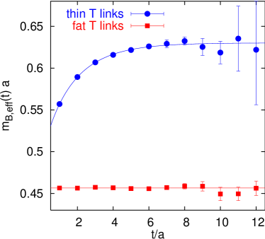
Figure 1: Comparison of effective masses of static-light correlation functions, obtained employing static actions with and without fat temporal links. The wave function has been optimized to yield best ground state overlap for the fat link static action. SET and HPA have been applied in both cases.

In Figure 1 we plot effective masses,

$$m_{X,\mbox{{\scriptsize eff}}}(t)=a^{-1}\ln\frac{C_{X}(t)}{C_{X}(t+a)},$$ (41)

of static-light mesons with and without fat time links. $C_{B}(t)$ stands for the static-light correlation function. The curves correspond to one- and two-exponential fits to the fat and thin link data, respectively. Note that the use of SET and HPA techniques (described in Sec. III.3 below) was essential for achieving the high signal quality. The new static action shifts the mass by an amount, $\delta m=0.174(7)\,a^{-1}$. The absolute statistical errors of the correlation function increase somewhat, however, the relative statistical errors are reduced, in particular at large times as the signal falls off less steeply. This in turn results in a reduction of the error of the effective masses, in particular at large $t$. The Figure also illustrates that we are able to achieve an excellent overlap with the physical ground state.

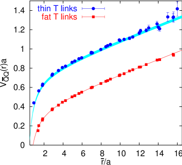
Figure 2: Comparison of the $\overline{Q}Q$ potential in lattice schemes with and without fat temporal links, in both cases for $t_{\min}/a=5$. String breaking is expected to take place around $\overline{r}=r_{c}\approx 15\,a$ but this is not visible from the Wilson loop data alone. The curve represents a funnel fit to the fat link data and the error band is this parametrization shifted upwards by the amount $2\delta m$, where $a\delta m=0.174(7)$.

In Figure 2 we compare the static potentials as calculated from the Wilson loop operator $C_{QQ}(t)$ alone, with and without fat time links. These potentials have been obtained from single exponential fits with $t_{\min}/a=5$. The curve corresponds to a funnel-type $r$-dependence with fit range $4a\leq\overline{r}\leq 13a$. String breaking is expected around $\overline{r}=r_{c}\approx 15\,a$. However, this is not seen in the data. The error band represents our expectation for the thin link potential, obtained from the respective static-light mass shift $\delta m$, as determined above. We find consistency.

The extended static action leaves the absolute errors of the correlation functions basically constant but still improves the signal exponentially. As a result, the effective mass errors are reduced impressively, by a factor of about five throughout..

III.3 All-to-all propagator techniques

The requirement of quark propagators from all source to all sink locations is obvious: within the $C_{BB}$ element of the correlation matrix, Eq. (29), we encounter light quark propagators starting from different source positions. Moreover, we can reduce the notorious noise levels of disconnected (and of some connected) diagrams; all-to-all propagators allow for the full exploitation of translational invariance, increasing the accuracy of the entire correlation matrix.

Since the propagator $M^{-1}$, Eq. (14), has $12V\times 12V$ components (in our case $V=24^{3}\times 40$), direct evaluation would be prohibitively expensive, both in terms of computer time and of memory. However, the correct result can also be obtained by combining the truncated eigenmode approach Neff:2001zr ; Schilling:2004kg ; Setoodeh:1988ds (TEA) with stochastic estimator techniques (SET). Where possible, we improve both, the convergence of TEA and the statistical errors of SET, by employing the hopping parameter acceleration (HPA).

For completeness we introduce these three techniques (TEA, SET and HPA) and their implementation in the following subsections. We conclude by comparing numerical data obtained by use of combinations of these methods.

III.3.1 Truncated eigenmode approach (TEA)

The fermionic propagator is the inverse of the Wilson Dirac matrix $M$ of Eq. (14). However, $M$ is not Hermitian which is why we define,

$$Q=\gamma_{5}M.$$ (42)

The relation $M^{\dagger}=\gamma_{5}M\gamma_{5}$ implies Hermiticity of $Q=Q^{\dagger}$. We calculate the smallest $n=200$ (real) eigenvalues $q_{i}$ and corresponding orthonormal eigenvectors $|u_{i}\rangle$, $i=1,\ldots,n$,

$$Q|u_{i}\rangle=q_{i}|u_{i}\rangle\quad,\quad\langle u_{i}|u_{j}\rangle=\delta_{ij}.$$ (43)

This is done by means of the parallel implicitly restarted Arnoldi method (IRAM) with Chebychev acceleration Neff:2001zr , using the PARPACK library arnoldi . We can now approximate,

$$Q^{-1}\approx\sum_{i=1}^{n}|u_{i}\rangle q_{i}^{-1}\langle u_{i}|.$$ (44)

Obviously, $M^{-1}=Q^{-1}\gamma_{5}$. With this truncated eigenmode approach (TEA), we have reduced a $12V\times 12V$ problem to a $12V\times 12n$ problem.

Another nice feature of this procedure is that there is no critical slowing down of the algorithm as the quark mass is reduced. However, the difference between the left and right hand sides of Eq. (44) is systematic. One can in principle estimate this bias from the convergence properties under variation of $n$ Neff:2001zr . In the present context we will render the result exact by stochastically estimating the remainder, replacing the systematic error by a statistical uncertainty. For this purpose, it is useful to define the projection operator ${\mathcal{P}}_{n}$, onto the basis spanned by the first $n$ eigenvectors,

$${\mathcal{P}}_{n}=\sum_{i=1}^{n}|u_{i}\rangle\langle u_{i}|.$$ (45)

Note that for $n$ smaller than the rank of $Q$, this basis is truncated and hence incomplete: ${\mathcal{P}}_{n}\neq{\mathbf{1}}$. However, $[Q,{\mathcal{P}}_{n}]=0$. We can also define the projector onto the orthogonal subspace, ${\mathbf{1}}-{\mathcal{P}}_{n}$.

III.3.2 Stochastic estimator techniques (SET)

Stochastic estimator techniques have been applied by various groups in the past Bitar:bb ; Bernardson:yg ; Dong:1995rx ; Eicker:1996gk ; Thron:1997iy ; Wilcox:1999ab ; Michael:1999nq ; Struckmann:2000bt ; McNeile:2004wu . We introduce the following notation,

$$\overline{O}=\frac{1}{N}\sum_{j=1}^{N}O^{j}.$$ (46)

$N$ denotes the number of “stochastic estimates”. Let $|\eta^{i}\rangle$, $i=1,\ldots,N$ be random vectors with the properties,

$$\overline{|\eta\rangle}=O(1/\sqrt{N}),$$ (47)

$$\overline{|\eta\rangle\langle\eta|}={\mathbf{1}}+O(1/\sqrt{N}).$$ (48)

These requirements are for instance met if the $12V$ components are numbers $e^{i\phi}$, with the uncorrelated phases $\phi\in\{\pm\pi/4,\pm 3\pi/4\}$ randomly selected. We employ such a complex ${\mathbb{Z}}_{2}$ noise, where our random vectors take values over the entire four-volume, flavour and colour.

If we solve the linear system,

$$Q|s^{i}\rangle=|\eta^{i}\rangle,$$ (49)

for $|s^{i}\rangle$ then, for large $N$, we can substitute [Eq. (48)],

$$Q^{-1}\approx\overline{|s\rangle\langle\eta|}.$$ (50)

Note that in our study we actually invert $A=M^{\dagger}M=Q^{2}$ and then obtain $Q^{-1}$ by multiplying the solution with $Q$. This allows for more flexibility: for instance the Roma smearing technique deDivitiis:1995pv , which amounts to the replacement $Q^{-1}\mapsto A^{-1}$ within hadronic Green functions, can readily be implemented. It can then be shown by means of spectral decompositions that in many cases the ground state mass remains unaffected deDivitiis:1995pv . In the present context we have made use of this method, in addition to standard smeared-smeared and smeared-local correlation functions, within the optimization procedure of the static-light creation operator. Unfortunately, Roma-smearing turns out not to be applicable to the $B\overline{B}\leftrightarrow\overline{Q}Q$ mixing problem.

The sparse linear system of Eq. (49) is solved by means of the BiCGstab2 algorithm Frommer:vn . Unlike in Eq. (44) where the bias was systematic, the difference between the approximation of Eq. (50) and the exact result is purely statistical and reduces like $1/\sqrt{N}$. In order to limit the computational effort, $N$ should not be chosen overly large. However, the noise level from SET should at least match the one from the (finite) sampling of gauge configurations. In general, the optimal balance in both samplings will also depend on the observable in question and on the methods employed.

We can estimate the difference between the TEA approximation and the true result by means of SET. The smaller this difference, the smaller the statistical errors will be that are introduced by SET. Hence TEA can be employed to reduce the variance of SET. We project the right hand side of Eq. (50) into the subspace which is orthogonal to the TEA eigenvectors:

$$(1-{\mathcal{P}}_{n})Q^{-1}(1-{\mathcal{P}}_{n})\approx\frac{1}{N}\sum_{j=1}^{N}(1-{\mathcal{P}}_{n})|s^{j}\rangle\langle\eta^{j}|(1-{\mathcal{P}}_{n}).$$ (51)

In practice this is done by calculating and storing,

$$|\tilde{s}^{j}\rangle = |s^{j}\rangle-\sum_{i=1}^{n}|u_{i}\rangle\langle u_{i}|s^{j}\rangle,$$ (52)

$$|\tilde{\eta}^{j}\rangle = |\eta^{j}\rangle-\sum_{i=1}^{n}|u_{i}\rangle\langle u_{i}|\eta^{j}\rangle.$$ (53)

Then,

$$M^{-1}\approx\left[\sum_{i=1}^{n}|u_{i}\rangle q_{i}^{-1}\langle u_{i}|+\frac{1}{N}\sum_{j=1}^{N}|\tilde{s}^{j}\rangle\langle\tilde{\eta}^{j}|\right]\gamma_{5}.$$ (54)

Note that there is no systematic error on finite-$N$ approximants but only a statistical $O(1/\sqrt{N})$ uncertainty. In the present context we found $N=50$, combined with $n=200$, to suffice for calculating $C_{QB}(t)$ and static-light meson correlators. Within the two diagrams contributing to $C_{BB}(t)$, it is necessary to choose two independent random sources as in either case there exist the same two possibilities of connecting sources with sinks. In these cases we calculate the SET corrections for the two respective propagators independently, with $N=25$ random sources each. Subsequently, we interchange the two sets of random sources to increase the statistics at little computational overhead. Such “recycling” has been pioneered by the Dublin group Cais:2004ww .

As long as we are only interested in using SET to remove the bias from TEA for a fixed $n$ we can in principle solve Eq. (49) within the orthogonal subspace only, substituting the random sources $|\eta^{j}\rangle$ on the right hand side with $|\tilde{\eta}^{j}\rangle$. We attempted this but found no advantage in terms of real cost in computer time. This of course might change at smaller quark masses or with different light quark actions. However, having random source solutions at our disposal that are independent of the TEA allows for more flexibility. For instance, not all physical states will be dominated by the lowest lying eigenmodes of $Q=\gamma_{5}M$. In particular, the TEA contribution to $C_{BB}^{\rm con}(t)$ turned out to be tiny, such that in the end we reduced the cost to compute $C_{BB}^{\rm con}(t)$, by employing a stand-alone SET.

Needless to say that, once we have calculated all-to-all propagators, Wuppertal smearing, Eq. (36), can be implemented. In principle, one could even variationally optimize the smearing function Draper:1993qj , for instance after fixing to Coulomb gauge. However, our smearing function turned out to be already so highly optimized that further gain was too hard to achieve.

III.3.3 Hopping parameter acceleration (HPA) of TEA and SET

The main motivation of complementing SET with TEA is to reduce the signal that needs estimation and hence the stochastic errors. One might ask if it is possible to further facilitate the low eigenvalue dominance, accelerating the convergence of TEA (and of SET). This is indeed possible by applying what we call the hopping parameter acceleration (HPA).

We rewrite the fermionic matrix Eq. (14) as,

$$M={\mathbf{1}}-\kappa D.$$ (55)

For sufficiently small hopping parameter values $\kappa<\kappa_{c}$, one can expand,

$$M^{-1}=\sum_{i=0}^{\infty}(\kappa D)^{i}=\sum_{i=0}^{k-1}(\kappa D)^{i}+(\kappa D)^{k}M^{-1},$$ (56)

where $k\geq 1$. The idea now is that for distances between source and sink that are bigger than $k$ lattice spacings the first term on the right hand side does not contribute. This can readily be seen as follows: as $D$ only connects nearest space-time neighbours [and ${\bf 1}=(\kappa D)^{0}$ only contains diagonal entries], the sum vanishes within elements $M_{xy}^{-1}$ if $\sum_{\mu}|x_{\mu}-y_{\mu}|/a\geq k\geq 1$. $M_{xy}^{-1}$ can be replaced by $[(\kappa D)^{k}M^{-1}]_{xy}$. This means that $Q^{-1}_{xy}=[(\kappa D)^{k}Q^{-1}]_{xy}$. With $M|r_{i}\rangle=\mu_{i}|r_{i}\rangle$, $\langle l_{i}|M=\mu_{i}\langle l_{i}|$, where $\mu_{i}$ are the eigenvalues of $M$, Eq. (44) can be substituted by,

$$Q^{-1}_{xy}=M^{-1}_{xy}\gamma_{5}\approx\sum_{i=1}^{n}\langle x|r_{i}\rangle(1-\mu_{i})^{k}\mu_{i}^{-1}\langle l_{i}|y\rangle\gamma_{5},$$ (57)

where again $k$ is smaller or equal to the number of links separating source from sink. For large $k$, contributions from big eigenvalues of $M$ are suppressed and the expression becomes all the more dominated by low lying eigenmodes. Hopefully, the dominance in terms of low eigenmodes of $M$ will then also apply to low eigenmodes of $Q$.

In fact we do not only find HPA to improve TEA but the main effect of HPA is with respect to SET: the cancellation of stochastic noise is accelerated if the number of contributions to the stochastic average is reduced. Short-distance noise is accompanied by larger amplitudes than large-distance noise and hence its cancellation requires a comparatively larger number of noise vectors. HPA explicitly eliminates such short-distance contributions.

The benefit from HPA will increase with larger temporal or spatial distances. Unfortunately, in the limit of light quark masses, as $\kappa$ approaches $\kappa_{c}$, the quark propagator will decay less rapidly with the distance and the explicit treatment of the first few terms within the hopping parameter expansion will have less of an effect. This is also obvious from the reduced convergence of the hopping parameter expansion at small quark masses. In this case we would however expect a better convergence of the TEA contribution in the first place.

Note that HPA exploits the ultra-locality of the Wilson action and does not generalize for instance to the Neuberger action Neuberger:1997fp . Again, this might be compensated for, by a faster convergent TEA approximation, due to the improved chiral properties of the chiral actions, in particular at small quark masses. In contrast, the “dilution” method advocated in Ref. Cais:2004ww will still be applicable in a setting with chiral fermions, reducing the variance of SET for the very same reasons as HPA does.

By applying HPA to the whole matrix, cf. Eq. (54), we exploit both effects, the improvement of the low eigenvalue dominance and the variance reduction of SET:

$$M^{-1}\approx\left(\kappa D\right)^{k}\left[\sum_{i=1}^{n}|u_{i}\rangle q_{i}^{-1}\langle u_{i}|+\frac{1}{N}\sum_{j=1}^{N}|\tilde{s}^{j}\rangle\langle\tilde{\eta}^{j}|\right]\gamma_{5},$$ (58)

where, as above, $ka$ is the lattice-distance between source and sink. Again, the above equation is exact up to statistical $O(1/\sqrt{N})$ corrections.

Unfortunately, due to the size of our smearing function, we cannot employ HPA for propagators along spatial separations, i.e. within $C_{QB}(t)$ or within $C_{BB}^{\rm con}(t)$. However, $C_{BB}^{\rm dis}(t)$ benefits from this technique as do static-light correlation functions. One way of extending it to the before-mentioned elements is to cut off the radius of the smearing function. Such a cut-off, in conjunction with an iterative smearing method, is hard to implement. One way out would be to work in Coulomb gauge with fixed weight-factors Draper:1993qj . Another possibility is the implementation of a rotationally non-invariant smearing function. But in this case it turned out to be difficult to sustain an acceptable ground state overlap.

III.3.4 Comparative study of SET, TEA and HPA

We demonstrate the impact of the above methods for the example of the static-light meson mass, in the scenario of the fat link static action described in Sec. III.2.2. We also verify the potential of HPA for the example of $C_{QB}(t)$, however, without smearing (see above).

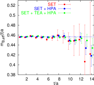
Figure 3: Effective static-light masses, obtained with SET alone, with HPA SET and with all three methods combined.

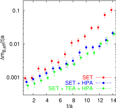
Figure 4: The errors of effective static-light masses, obtained with SET alone, with HPA SET and with all three methods combined.

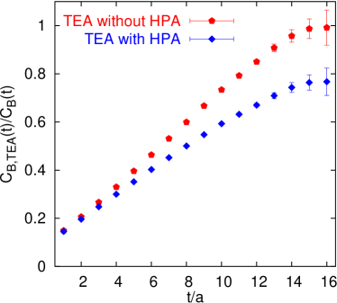
Figure 5: The relative magnitude of the TEA contribution within the static-light correlation function, with and without HPA.

In Figure 3 we display effective masses Eq. (41), obtained with SET alone as well as with HPA SET, and after explicitly calculating the contribution from the first 200 eigenmodes (TEA). Note that the ordinate covers a huge $t$-range, up to a distance $t\approx 1.2$ fm. Also note the magnified scale of the abscissa, covering the window $0.9\,\mbox{GeV}<m_{B,{\rm eff}}<1.26$ GeV. In particular at large times, HPA impressively reduces the errors and TEA results in some additional improvement. This is quantified in Figure 4, where we display the respective statistical errors themselves. Note the logarithmic scale. For instance, at $t=8a$ HPA reduces the SET error to about one third of its original value while TEA yields another $\approx 20$ % reduction. Since the effective mass is approximately independent of $t$ the absolute errors displayed are proportional to the relative errors which (as is obvious from the Figure) grow exponentially with $t$. Fortunately, both, HPA and TEA reduce the amplitude and the exponent governing this error increase, resulting in an exponential improvement at large times.

In Figure 5 we see that the static-light correlation function at large times becomes dominated by TEA. Without HPA this dominance seems to be achieved earlier than with HPA: the sea quark mass still appears too heavy for HPA to significantly enhance the low eigenvalue dominance of $Q=\gamma_{5}M$, for the correlation function in question. However, the seemingly perfect agreement for the stand-alone TEA case of the displayed ratio at large $t$ with one is largely accidental. Increasing the number of eigenvectors on one configuration revealed that TEA tends to overshoot the exact result, before converging towards it. HPA reduces this tendency. Note that HPA cannot be applied to the SET part alone, within the SET plus TEA combination.

In the HPA case TEA also results in an impressive reduction of the signal that remains to be estimated. However, a comparison between SET plus HPA and SET plus HPA plus TEA reveals that the additional error reduction due to TEA is only moderate. After HPA the SET error is already at the level of the statistical fluctuations between gauge configurations and of a comparable size to the (non-stochastical) TEA error. In this situation, substituting part of one signal by the other leaves the resulting statistical error largely unaffected. This would have been different for a larger statistical sample or at smaller sea quark masses.

Finally, we wish to investigate the effect of HPA on correlators as a function of spatial source-sink separations. This is done for the example of $C_{QB}(t)$, without smearing.

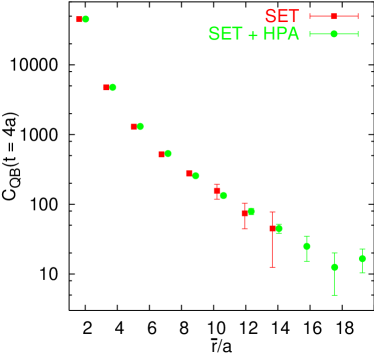
Figure 6: The effect of HPA on SET for the example of $C_{QB}$ at $t=4a$, as a function of the distance $\overline{r}$. The normalization is arbitrary and we have employed local sources and sinks.

In Figure 6 we show the local-local $C_{QB}$ matrix element at fixed $t=4a$ as a function of $\overline{r}$, both for SET alone and for HPA SET. All distances are along the spatial diagonal, i.e. when increasing $\overline{r}$ by $\approx\sqrt{3}a$, the exponent $k$ increases by three units. At our largest separation $\overline{r}/a\approx 11\sqrt{3}\approx 19.05$ we have $k=33$! The error reduction factors turn out to be fairly time-independent. At the largest distance accessible without HPA $\overline{r}/a\approx 8\sqrt{3}\approx 13.9$, the error reduction is almost five-fold. Potentially, this should be even more impressive for $C_{BB}^{\rm con}$, within which two spatial light quark propagators appear. Unfortunately, the method cannot be combined with our present smearing function, which is essential for accessing the physical ground states.

III.4 Notation and spectral decomposition

In order to set the stage for the interpretation of our numerical data, we detail in this section our notations in connection with the spectral decompositions for the different matrix elements, Eq. (29). We will assume an infinite extent in time direction of the lattice and asymptotic behaviour of all correlators. We often suppress the distance dependence, ${\mathbf{r}}$, from the expressions.

We define $B_{i}\overline{B}_{j}$ pair creation operators ${\mathcal{B}}_{ij}$. These create a light antiquark of flavour $j$ and a quark of flavour $i$, besides the static sources. The states created by ${\mathcal{B}}_{ij}$, $i\neq j$, constitute a subset of the flavour non-singlet (“$I=1$”) states. The remaining $n_{f}-1$ $I=1$ states are given by traceless linear combinations of the ${\mathcal{B}}_{ij}$ diagonal elements. In addition, a flavour singlet ($I=0$) creation operator, ${\mathcal{B}}_{s}=\frac{1}{\sqrt{n_{f}}}\sum_{i=1}^{n_{f}}{\mathcal{B}}_{ii}$, can be constructed. ${\mathcal{B}_{a}}$ represents one of the $n_{f}^{2}-1$ members of the class of $I=1$ operators.

Flavour singlet states are created both, by ${\mathcal{B}}_{s}$ and by ${\mathcal{Q}}$, the operator that only contains static quark-antiquark spinors. We remind the reader of the definitions Eq. (18) and Eq. (22), $|Q\rangle={\mathcal{Q}}|0\rangle$, $|B\rangle={\mathcal{B}}_{s}|0\rangle$, with vacuum state $|0\rangle$. Obviously, $\langle Q|0\rangle=\langle B|0\rangle=0$. We denote the orthonormal eigenstates in the flavour singlet sector as $|n\rangle$, $n=1,2,\ldots$, with energies $E_{n+1}\geq E_{n}$.

For the labelling of the $I=1$ sector, we follow the convention of Eq. (23) and define, $|B_{a}\rangle={\mathcal{B}}_{a}|0\rangle$. All flavour non-singlet eigenstates share the same energy spectrum, $E_{n}^{a}$. We label eigenstates of the $I=1$ sector, within the class of states with energy $E_{n}^{a}$, by $|n_{a}\rangle$, $n=1,2,\ldots$.

Just for annotation at this point: while the $I=1$ states decouple from the $I=0$ states there will still be mixing between $I=1$ states and two meson states, containing for instance a $\overline{Q}Q$ plus a $\pi$. A calculation of the $I=1$ correlation matrix, analogous to the $I=0$ sector, is beyond the scope of the present paper.

Note that we smear the $B_{\mathbf{r}}\overline{B}_{\mathbf{0}}$ creation operator at position ${\mathbf{0}}$ while the sink is smeared at ${\mathbf{r}}$. This means that the creation operator ${\mathcal{B}}_{s|a}^{i}=\overline{Q}_{{\mathbf{r}}}\gamma_{5}q_{{\mathbf{r}}}\bar{q}_{{\mathbf{0}}}\Phi\gamma_{5}Q_{{\mathbf{0}}}$ within Eq. (21), where the smearing function $\Phi$ acts on the quark at position ${\mathbf{0}}$, is not the Hermitian adjoint of the annihilation operator, ${\mathcal{B}}_{s|a}^{f}\neq{\mathcal{B}}_{s|a}^{i\dagger}$. The subscripts “$i$” and “$f$” stand for initial and final, respectively. Hence, strictly speaking, one has to distinguish between $\langle B^{f}_{(a)}|$ and $|B^{i}_{(a)}\rangle$. From a practical point of view, the highly satisfying ground state dominance of our data renders this distinction obsolete.

We can decompose,

$$|Q\rangle=\sum_{n>1}\langle n|Q\rangle|n\rangle=\sum_{n}Q_{n}|n\rangle,$$ (59)

$$|B^{i}\rangle=\sum_{n>1}\langle n|B^{i}\rangle|n\rangle=\sum_{n}B^{i}_{n}|n\rangle,$$ (60)

where

$$\sum_{n}|Q_{n}|^{2} = \langle Q|Q\rangle,$$ (61)

$$\sum_{n}{B^{f}_{n}}^{*}B^{i}_{n} = \langle B^{f}|B^{i}\rangle,$$ (62)

$$\sum_{n}Q_{n}^{*}B^{i}_{n} = \sum_{n}{B^{f}_{n}}^{*}Q_{n}=0.$$ (63)

Using these notations, the matrix elements Eq. (29) read (neglecting the overall energy off-set $2m_{Q}$),

$$C_{QQ}(t) = \mbox{ \begin{minipage}{16.0pt}\includegraphics[width=16.0pt]{w11.ps}\end{minipage}}=\sum_{n}|Q_{n}|^{2}e^{-E_{n}t},$$ (64)

$$C_{QB}(t) = \sqrt{n_{f}}\mbox{ \begin{minipage}{16.0pt}\includegraphics[width=16.0pt]{w12.ps}\end{minipage}}=\sum_{n}\mbox{Re}(Q_{n}^{*}B^{i}_{n})e^{-E_{n}t},$$ (65)

$$C_{BB}(t) = \mbox{ \begin{minipage}{16.0pt}\includegraphics[width=16.0pt]{w22d.ps}\end{minipage}}-n_{f}\mbox{ \begin{minipage}{16.0pt}\includegraphics[width=16.0pt]{w22c.ps}\end{minipage}}=\sum_{n}\mbox{Re}({B^{f}_{n}}^{*}B^{i}_{n})e^{-E_{n}t},$$ (66)

$$C_{BB}^{\rm dis}(t) = \mbox{ \begin{minipage}{16.0pt}\includegraphics[width=16.0pt]{w22d.ps}\end{minipage}}=\sum_{n}\mbox{Re}({B^{f*}_{a,n}}B^{i}_{a,n})e^{-E_{n}^{a}t}.$$ (67)

Note that $\mbox{Re}(Q_{n}^{*}B^{i}_{n})=\mbox{Re}(Q_{n}^{*}B^{f}_{n})$.

The normalization of our correlation matrix is such that $C_{\alpha\beta}(t)>0$ for $t\rightarrow\infty$, i.e. the ground state amplitudes are always positive. However, within $C_{QB}$ and $C_{BB}$, excited state amplitudes can be negative.

For $r<r_{c}$ the ground state $|1\rangle$ will be dominated by a $|Q\rangle$-type component, whereas the first excitation $|2\rangle$ has a large $|B\rangle$ contribution. For $r>r_{c}$ this correspondence will interchange. We view a signal $C_{QB}\neq 0$ as an “explicit” signature for mixing while a verification of an $E_{1}$ signal in $C_{QQ}(t)$ at $r>r_{c}$ (string decay) or within $C_{BB}(t)$ at $r<r_{c}$ will be referred to as an “implicit” mixing effect.

IV Investigation of individual matrix elements

We set the stage for the investigation of the mixing problem by comparing individual matrix elements to theoretical expectations. We first discuss $C_{BB}$ and then combinations of different components of the correlation matrix, before we attempt to detect implicit mixing effects.

IV.1 Large time asymptotics

We remark that $C_{BB}(t)$ contains a disconnected and a connected contribution. The disconnected term coincides with the $I=1$ diagram Eq. (67), and the states it couples to are orthogonal to the $I=0$ sector: any implicit mixing can only be mediated through $C_{BB}^{\rm con}$. This means that at $0<r<r_{c}$,

$$C_{BB}(t)\rightarrow-C_{BB}^{\rm con}(t)\quad(t\rightarrow\infty):$$ (68)

the connected diagram will dominate at asymptotically large $t$. This is in contrast to the situation at small to moderately large times, where the overlaps $|B_{1}|\ll|B_{2}|$ [cf. Eqs. (60) and (66)] warrant a disconnected diagram dominance. We shall see below that Eq. (68) in fact turns out to be valid for any $r>0$, including $r>r_{c}$.

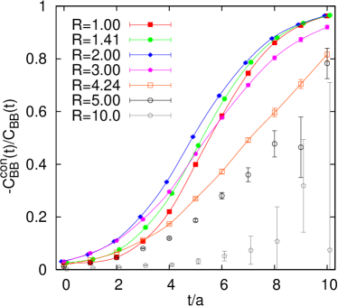
Figure 7: The ratio $-C_{BB}^{\rm con}/C_{BB}$ as a function of $t$ for various $r=Ra$. The splines are drawn to guide the eye.

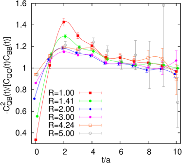
Figure 8: The ratio $-C_{QB}^{2}/(C_{QQ}C_{BB})$ as a function of $t$ for various $r=Ra$. The splines are drawn to guide the eye.

We investigate the above expectation in Figure 7, where we plot ratios $-C_{BB}^{\rm con}(t)/C_{BB}(t)$ as functions of $t$ for a few $R=r/a$ values. Note that $Ra=6a\approx r_{0}\approx 0.5$ fm. As expected, at large $t$, this ratio approaches one. Note that $r=0$ represents a special case. In this limit, the $\overline{Q}Q$ and the $B\overline{B}$ sectors decouple and Eq. (68) does not hold. As a consequence, the asymptotic limit is reached faster for $r=2a$ than for $r=a$ which is adjacent to $r=0$. For $r>2a$, the speed of convergence decreases again: the gap between the two energy levels $E_{1}$ and $E_{2}$ reduces as a function of $r$ and hence the limit is approached less and less rapidly in $t$. At large $r$ the signal vanishes in noise, before it can approach unity.

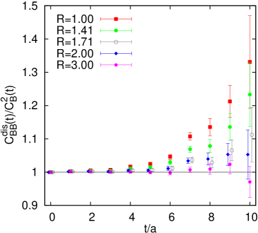
Figure 9: The ratio $C_{BB}^{\rm dis}/C_{B}^{2}$ as a function of $t$ for small $r=Ra$.

From Eqs. (64) – (66) it is expected that at asymptotically large times, for all $r>0$,

$$|C_{QB}(t)|^{2}\rightarrow C_{QQ}(t)C_{BB}(t)\quad(t\rightarrow\infty).$$ (69)

In Figure 8 we verify this expectation for some selected distances. The disconnected contribution to $C_{BB}$ has to decay faster than the connected contribution. Otherwise the corresponding $n_{f}$, colour and Dirac factors would be incompatible with Eq. (69). Hence Eq. (68) above is not only valid at $r<r_{c}$ but for any distance $r>0$.

In particular this means that at large $t$,

$$C_{QB}^{2}(t)\rightarrow-C_{QQ}(t)C_{BB}^{\rm con}(t),$$ (70)

or, diagrammatically,

$$\mbox{ \begin{minipage}{16.0pt}\includegraphics[width=16.0pt]{w12.ps}\end{minipage}}\times\mbox{ \begin{minipage}{16.0pt}\includegraphics[width=16.0pt]{w21.ps}\end{minipage}}\rightarrow-\mbox{ \begin{minipage}{16.0pt}\includegraphics[width=16.0pt]{w11.ps}\end{minipage}}\times\mbox{ \begin{minipage}{16.0pt}\includegraphics[width=16.0pt]{w22c.ps}\end{minipage}}\quad,$$ (71)

again for any $r>0$. This limiting behaviour is approached faster in time than Eq. (69) above.

Both sides of Eq. (69) are dominated by the ground state contribution $|1\rangle$, which results in an exponential decay $\propto e^{-2E_{1}t}$. At $r<r_{c}$, $C_{QQ}$ couples more strongly to this term than $C_{BB}$. This interchanges at $r>r_{c}$, where the ground state is dominantly contained within the $C_{BB}$ sector. The decoupling of $C_{QB}$ from the $I=1$ sector implies, $E_{1}\leq E_{1}^{a}$: the $I=0$ ground state energy cannot be larger than the lowest $I=1$ energy level, at any distance $r>0$.

Finally, we compare $C_{BB}^{\rm dis}(t)$ to the static-light correlation function $C_{B}(t)$. If the $B$-mesons at positions ${\bf 0}$ and ${\bf r}$ did not interact with each other then the ratio $C_{BB}^{\rm dis}(t)/C_{B}^{2}(t)$ would be unity. The $I=1$ $B\overline{B}$ state would merely act like the sum of two isolated $B$ mesons. We investigate this ratio in Figure 9 and find this scenario to be valid within our statistical resolution for $r\geq 2\sqrt{2}a\approx 0.23$ fm. The increase of this ratio at large $t$ for small $r<2\sqrt{2}a$ can be attributed to an increased overlap of the creation operator with the $\overline{Q}Q\pi$ $I=1$ ground state, see also Sec. V.4.

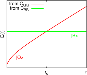
Figure 10: Expected spectrum in the absence of mixing effects. The ground state at small $r$ has no overlap with the $|B\rangle$ sector but is only contained within $C_{QQ}$. At $r>r_{c}$ the ground state is only visible in $C_{BB}$.

Figure 11: Effective masses. The solid symbols are from $C_{BB}(t)$, the open symbols from the Wilson loop $C_{QQ}(t)$. The horizontal line corresponds to twice the mass of a static-light meson.

IV.2 Implicit detection of mixing effects

We investigate whether the actual ground state energy level is visible in $C_{BB}(t)$ at $r<r_{c}$ or in $C_{QQ}(t)$ at $r>r_{c}$. For this purpose, we study the large $t$ behaviour of effective masses, Eq. (41). The qualitative expectation in the absence of any mixing is sketched in Figure 10: at $r<r_{c}$ the ground state can only be detected within $C_{QQ}$, while at $r>r_{c}$ the ground state energy is given by the large $t$ behaviour of $C_{BB}$ and will not be visible from $C_{QQ}$. Implicit mixing means that the $C_{QQ}$ and $C_{BB}$ effective masses share the same ground state. At $r<r_{c}$ the $C_{QQ}$ effective mass is expected to plateau at smaller $t$ values than the $C_{BB}$ effective mass. At $r>r_{c}$ the ground state then will become dominated by the $|B\rangle$ contribution and hardly be visible in $C_{QQ}$.

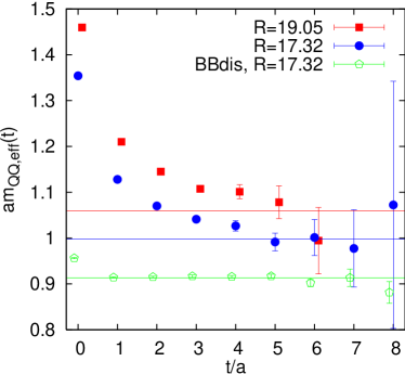
Figure 12: Effective masses from the Wilson loop $C_{QQ}$. The lowest horizontal line is $2m_{B}$. The other two horizontal lines denote the central values of the respective excited state expectations from a global linear plus Coulomb fit to the potential from $2<R\leq 13$ Wilson loop data. The open pentagons, from $C_{BB}^{\rm dis}$, demonstrate the plateau quality within the $C_{BB}$ sector.

We display the situation for small $r$ in Figure 11. The open symbols, calculated from Wilson loops $C_{QQ}$, exhibit good and early plateaus. The solid symbols, which correspond to the matrix element $C_{BB}$, start out from values, similar to the mass of two static-light mesons, but then decay towards the respective lower lying states, clearly signalling implicit mixing effects! Note that as $C_{BB}^{\rm dis}$ alone only projects onto the $I=1$ sector, this effect is entirely due to the $C_{BB}^{\rm con}$ contribution, see Figure 7.

We are also tempted to verify implicit string breaking at large $r$. To this end, in Figure 12 we examine effective Wilson loop masses for two distances $r>r_{c}\approx 15a$: $r/a=10\sqrt{3}\approx 17.32$ and $r/a=11\sqrt{3}\approx 19.05$. The upper two horizontal lines denote the respective plateau value expectations from a global linear plus Coulomb fit to the potential as obtained from Wilson loops, in the region without string breaking, $\overline{r}<11\,a<r_{c}$. We wish to see the data to deviate from this expectation, towards the lowest line, that corresponds to $2m_{B}$. We conclude that we see no implicit indications of string breaking in the Wilson loop data.

We also demonstrate the quality of the effective mass plateau within the $C_{BB}$ sector in Figure 12 (open pentagons). Here, in the interest of small error bars, we neglected the $C_{BB}^{\rm con}$ correction to the masses. As expected, the $C_{BB}^{\rm dis}$ effective mass data agree with twice the static-light mass. We remark that we also find $E_{1}\approx E_{1}^{a}$ within errors, in agreement with the level ordering expectation, $E_{1}\leq E_{1}^{a}$.

The absence of an indication of implicit string breaking at large $r$ is no surprise since in a study of adjoint potentials in $2+1$ dimensional $SU(2)$ gauge theory Kratochvila:2003zj , this was only seen at physical times much bigger than ours. We shall address the question, at what $t$ values implicit string breaking should become visible, in Sec. V.3 below. We will see in Sec. V.1, where we also study explicit mixing effects, that mixing is indeed much smaller at $r>r_{c}$ than at $r<r_{c}$.

V Results

We present our analysis and results on the $I=0$ mixing angle and energy levels. We then discuss string breaking as well as transition rates, before we address the short distance behaviour of the energy levels, both within the $I=0$ and the $I=1$ sectors. As we only work at a fixed value of the lattice spacing, it is convenient to display all results in this section in lattice units, $a\approx 0.083$ fm, i.e. $a^{-1}\approx 2.37$ GeV.

V.1 The mixing analysis

Our creation and annihilation operators are highly optimized, such that the overlaps $Q_{n}=\langle n|Q\rangle$ and $B_{n}=\langle n|B\rangle$ are close to zero for $n\geq 3$. Hence, we base our analysis on the simplified mixing scenario,

$$|Q\rangle=a_{Q}\left(\cos\theta|1\rangle-\sin\theta|2\rangle\right),$$ (72)

$$|B\rangle=a_{B}\left(\sin\theta|1\rangle+\cos\theta|2\rangle\right),$$ (73)

truncating Eqs. (59) and (60) after $n=2$. In what follows, we abbreviate, $c_{\theta}=\cos\theta$ and $s_{\theta}=\sin\theta$. The identification, $Q_{1}=a_{Q}c_{\theta}$, $Q_{2}=-a_{Q}s_{\theta}$, $B_{1}=a_{B}s_{\theta}$ and $B_{2}=a_{B}c_{\theta}$ above guarantees that $\langle Q|B\rangle=0$, as well as positivity of all correlation matrix elements for large Euclidean times.

The ansatz Eqs. (72) – (73) implies that,

$$C_{QQ}(t) = a_{Q}^{2}\left[c_{\theta}^{2}\exp\left(-E_{1}t\right)+s_{\theta}^{2}\exp\left(-E_{2}t\right)\right],$$ (74)

$$C_{BB}(t) = a_{B}^{2}\left[s_{\theta}^{2}\exp\left(-E_{1}t\right)+c_{\theta}^{2}\exp\left(-E_{2}t\right)\right],$$ (75)

$$C_{QB}(t) = a_{Q}a_{B}s_{\theta}c_{\theta}\left[\exp\left(-E_{1}t\right)-\exp\left(-E_{2}t\right)\right].$$ (76)

We also determine the correlation functions at $t=0$. This enables us to implement the normalization, $C_{QQ}(0)=C_{BB}(0)=1$. In this case, the $a_{Q}$ and $a_{B}$ values, fitted at large $t$, can be interpreted as the overlaps of our respective trial wave functions with the $n\leq 2$ eigenstate sector, with optimal value, $a_{Q}^{2}=a_{B}^{2}=1$. While $a_{Q}^{2}\leq 1$, this is not necessarily so for $a_{B}^{2}$ as here additional exponentials can come in with negative weight.

We attempted to model corrections to Eqs. (74) – (76), by adding additional exponentials to our fits. The overlaps $\langle n|B\rangle$ for $n\geq 3$ were so tiny that, except at $r\leq 2a$, we were unable to detect any additional masses in the $C_{BB}$ channel. It was however possible to add an additional excitation to the $|Q\rangle$ channel. This exponential then also couples to the $C_{QB}$ element. Results of such eight parameter fits were very compatible with those of the simultaneous five parameter fits introduced above, with parameters $\theta,a_{Q},a_{B},E_{1}$ and $E_{2}$. However, these eight parameter fits were not stable at all distances. In contrast, the five parameter fits turned out to be very robust, such that the results presented here are based on the parametrization Eqs. (74)–(76). We also attempted six parameter fits, allowing $\theta$ to take two different values within Eq. (72) and Eq. (73). This however did not improve the $\chi^{2}/N_{DF}$ qualities and the two $\theta$-angles turned out to agree within errors. We conclude that the mixing scenario Eqs. (74)–(76) is preferred by the data.

For each $r$ we carefully checked the quality of the fits and the stability of the parameter values with respect to variations of the fit range. For each of the three matrix elements we determined a $t_{\alpha\beta,\min}$ value. $a_{B}$ turned out to be much closer to unity than $a_{Q}$ and we found, $t_{QQ,\min}\geq t_{QB,\min}\geq t_{BB,\min}$. The fit ranges that we employed in our final analysis are,

$$t_{QQ,\min}=4a,\,t_{QB,\min}=3a,\,t_{BB,\min}=2a \mbox{for}\quad\overline{r}>15.5a,$$ (77)

$$t_{QQ,\min}=t_{QB,\min}=4a,\,t_{BB,\min}=2a \mbox{for}\quad 15.5a\geq\overline{r}>13a,$$ (78)

$$t_{QQ,\min}=5a,\,t_{QB,\min}=4a,\,t_{BB,\min}=2a \mbox{for}\quad 13a\geq\overline{r}>12a,$$ (79)

$$t_{QQ,\min}=6a,\,t_{QB,\min}=5a,\,t_{BB,\min}=2a \mbox{for}\quad 12a\geq\overline{r}>8a,$$ (80)

$$t_{QQ,\min}=6a,\,t_{QB,\min}=5a,\,t_{BB,\min}=3a \mbox{for}\quad\overline{r}\leq 8a.$$ (81)

Table 1: The energy levels $E_{1}$ and $E_{2}$, as well as the mixing angle $\theta$, the overlaps $a_{Q}$ and $a_{B}$ and the transition rate $g$, defined in Eq. (100). Note that at $r=0$, $E_{1}=0$ and the ground state energy is, $a(E_{g}-2m_{B})=-0.59(17)$. $E_{2}$ denotes the first excitation above this state.

$\overline{r}/a$	$a[E_{1}-2m_{B}]$	$a[E_{2}-2m_{B}]$	$a[E_{2}-E_{1}]$	$\theta$	$a_{Q}$	$a_{B}$	$ag$
$r=0$	-0.913 (3)	0.021 (7)	0.934 (7)	0	1	0.978 (3)	0
1.365	-0.759 (4)	0.021 (7)	0.780 (8)	0.129 (2)	1.016(10)	0.985(11)	0.0996 (5)
1.442	-0.706 (4)	0.028 (5)	0.734 (7)	0.168 (2)	1.019(10)	0.995 (9)	0.1210 (5)
1.826	-0.648 (4)	0.035 (4)	0.683 (6)	0.196 (3)	1.022(10)	1.003 (7)	0.1304 (7)
1.855	-0.634 (4)	0.032 (5)	0.667 (7)	0.212 (3)	1.022(10)	1.000 (8)	0.1369 (6)
2.836	-0.539 (4)	0.036 (4)	0.575 (5)	0.239 (3)	1.025(11)	1.007 (6)	0.1323 (6)
2.889	-0.529 (4)	0.034 (4)	0.564 (5)	0.246 (3)	1.026(10)	1.005 (7)	0.1330 (6)
3.513	-0.489 (4)	0.033 (4)	0.522 (5)	0.239 (3)	1.021(10)	1.005 (6)	0.1199 (7)
3.922	-0.460 (4)	0.029 (4)	0.489 (5)	0.231 (3)	1.010(10)	1.002 (6)	0.1089 (6)
4.252	-0.444 (4)	0.030 (3)	0.474 (5)	0.221 (3)	1.001(11)	1.004 (5)	0.1014 (6)
4.942	-0.404 (3)	0.026 (4)	0.430 (4)	0.203 (2)	0.989 (9)	1.003 (5)	0.0849 (5)
5.229	-0.392 (3)	0.026 (4)	0.418 (4)	0.193 (2)	0.983 (9)	1.004 (6)	0.0787 (6)
5.666	-0.370 (4)	0.020 (3)	0.389 (5)	0.184 (3)	0.976(11)	0.996 (5)	0.0700 (4)
5.954	-0.360 (3)	0.019 (4)	0.379 (4)	0.177 (3)	0.955 (9)	0.997 (5)	0.0657 (6)
6.953	-0.315 (4)	0.016 (3)	0.331 (4)	0.163 (3)	0.941(12)	0.995 (5)	0.0531 (6)
6.962	-0.315 (3)	0.017 (4)	0.332 (4)	0.166 (3)	0.937 (8)	0.996 (6)	0.0542 (7)
7.079	-0.307 (4)	0.010 (3)	0.318 (4)	0.169 (3)	0.944(10)	0.984 (4)	0.0527 (5)
7.967	-0.273 (3)	0.010 (4)	0.283 (5)	0.170 (4)	0.917 (8)	0.986 (7)	0.0471 (6)
8.492	-0.252 (5)	0.008 (2)	0.260 (5)	0.172 (4)	0.907(15)	0.982 (2)	0.0439 (6)
8.680	-0.239 (5)	0.005 (2)	0.244 (5)	0.175 (5)	0.920(15)	0.978 (2)	0.0418 (8)
8.971	-0.222 (5)	0.006 (2)	0.228 (5)	0.181 (4)	0.926(13)	0.980 (2)	0.0405 (7)
9.905	-0.197 (7)	0.007 (2)	0.204 (7)	0.180 (5)	0.875(17)	0.982 (2)	0.0358 (8)
9.974	-0.187 (6)	0.006 (2)	0.193 (5)	0.186 (6)	0.891(17)	0.980 (2)	0.0351 (8)
10.408	-0.182 (9)	0.005 (2)	0.187 (9)	0.179(10)	0.849(24)	0.979 (2)	0.0327(10)
10.977	-0.145(11)	0.002 (2)	0.147(10)	0.202(16)	0.878(31)	0.977 (2)	0.0289 (8)
11.319	-0.145 (8)	0.006 (2)	0.150 (8)	0.191(11)	0.837(20)	0.980 (2)	0.0280 (8)
12.138	-0.119 (9)	0.005 (2)	0.125(10)	0.194(15)	0.811(23)	0.980 (2)	0.0235 (6)
12.733	-0.092 (7)	0.006 (1)	0.097 (7)	0.227(16)	0.814(15)	0.980 (2)	0.0214 (5)
13.869	-0.036 (6)	0.008 (2)	0.044 (5)	0.384(58)	0.823(14)	0.981 (2)	0.0151 (6)
14.147	-0.039 (5)	0.007 (2)	0.046 (5)	0.345(39)	0.792 (9)	0.981 (2)	0.0147 (5)
14.288	-0.032 (5)	0.007 (2)	0.039 (4)	0.395(49)	0.794(12)	0.981 (3)	0.0140 (6)
14.463	-0.026 (5)	0.007 (2)	0.033 (3)	0.498(71)	0.793(12)	0.978 (3)	0.0137 (6)
14.605	-0.016 (4)	0.009 (3)	0.025 (3)	0.59 (11)	0.801(12)	0.981 (2)	0.0115 (6)
14.704	-0.017 (4)	0.009 (3)	0.027 (2)	0.69 (11)	0.794(11)	0.977 (3)	0.0131 (5)
15.008	-0.011 (3)	0.011 (3)	0.022 (1)	0.87 (12)	0.784(11)	0.977 (2)	0.0110 (5)
15.176	-0.005 (3)	0.018 (5)	0.022 (3)	1.01 (12)	0.787(12)	0.981 (2)	0.0100 (7)
15.372	-0.003 (2)	0.027 (7)	0.030 (5)	1.204(78)	0.792(14)	0.980 (3)	0.0100 (6)
15.561	-0.002 (2)	0.027 (6)	0.029 (5)	1.15 (10)	0.771(14)	0.982 (2)	0.0109 (4)
15.600	-0.002 (2)	0.037 (8)	0.039 (8)	1.305(61)	0.793(15)	0.980 (2)	0.0100 (5)
17.331	0.001 (2)	0.095(13)	0.094(12)	1.501(12)	0.756(21)	0.981 (2)	0.0066 (5)
19.063	0.003 (2)	0.164(20)	0.161(20)	1.546 (4)	0.736(29)	0.982 (2)	0.0040 (4)

We determined the correlation matrix elements $C_{\alpha\beta}(t)$ for $0\leq t\leq 10$. However, the quality of the $C_{QQ}$ and $C_{QB}$ data only allowed us to use $t_{\max}=9$ for $\overline{r}\geq 12$. For the discussion of the individual matrix elements presented in the previous sections, we calculated jackknife and bootstrap errors. Both showed consistent results. Hence, in this more complicated mixing analysis we restrict ourselves to the jackknife method.

Prior to the fits we transformed the data:

$$C_{\alpha\beta}(t)\rightarrow C_{\alpha\beta}(t)/C_{B}^{2}(t).$$ (82)

This automatically normalizes the energy levels with respect to $2m_{B}$, removing the self energy $2m_{Q}$. In principle, this procedure bears the risk of introducing additional energy levels that are present in the static-light correlation function but not within the $\overline{Q}Q/B\overline{B}$ system. Figure 3 confirms nicely that at $t>a$ no such levels are statistically detectable. $C_{B}(0)$, however, turns out to be about 2 % larger than an exponential extrapolation down from $t\geq a$ suggests. We correct for this in the calculation of the overlaps $a_{Q}$ and $a_{B}$. The results for all fit parameters are summarized in Table 1.

$\theta$ is the mixing angle of the physical eigenstates $|1\rangle,|2\rangle$ with respect to the Fock basis $|Q\rangle,|B\rangle$, used in the simulation. We invert Eqs. (72) – (73), adapting the normalization $|Q\rangle\mapsto a_{Q}^{-1}|Q\rangle$, $|B\rangle\mapsto a_{B}^{-1}|B\rangle$:

$$|1\rangle = \cos\theta|Q\rangle+\sin\theta|B\rangle,$$ (83)

$$|2\rangle = -\sin\theta|Q\rangle+\cos\theta|B\rangle.$$ (84)

In our $t_{\alpha\beta}\geq t_{\alpha\beta,\min}$ analysis we effectively encounter this idealized picture and truncate the eigenbasis at $n=2$, which is supported by the data. However, we also truncate the Fock basis after the $\overline{Q}q\bar{q}Q$ sector. In general, the physical eigenstates will receive contributions from higher Fock states too and hence there will be a (slight) model dependence in the determination of $\theta$.

The limit ${\mathbf{r}}={\mathbf{0}}$ represents a special case. In this limit,

$$\mbox{ \begin{minipage}{16.0pt}\includegraphics[width=16.0pt]{w21.ps}\end{minipage}}\propto{\mathbf{0}}\cdot\langle\bar{q}_{0}\boldsymbol{\gamma}(1-\gamma_{4})q_{0}\rangle_{U}=0,$$ (85)

since $\langle\bar{q}\gamma_{i}q\rangle_{U}=\langle\bar{q}\gamma_{i}\gamma_{4}q\rangle_{U}=0$: the two $I=0$ eigenstates decouple and hence $\theta=0$. Moreover, $\langle W({\mathbf{0}},t)\rangle_{U}=const$, which means that the vacuum is the ground state. $\overline{Q}$ and $Q$ annihilate: $E_{1}(0)-2m_{B}=-2m_{B}$. The ground state overlap at this point is $a_{Q}=1$, by definition, and $C_{QB}$ is undefined. At $r=0$ we perform a two exponential fit for $t\geq a$ to $C_{BB}(t)$, with exponents $E_{g}$ and $E_{2}$. The lower mass (without subtracting $2m_{B}$) is $E_{g}=0.32(17)a^{-1}$ but with tiny overlap: $a_{g}^{2}=0.0045(15)$. This mass should coincide with the mass of two interacting pions or with the scalar $f_{0}$ mass, see also Sec. V.4 below. We have $2m_{\pi}=0.55(1)a^{-1}$ for two non-interacting pions while the mass of the lightest scalar is Bali:2000vr $m_{0^{++}}=0.71(6)a^{-1}$. Both values are compatible within two standard deviations with the fitted $E_{g}$ value above.

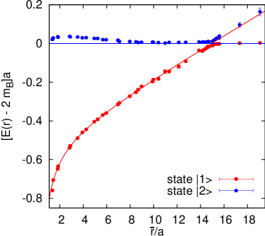
Figure 13: The two energy levels, as a function of $\overline{r}$, normalized with respect to $2m_{B}$ (horizontal line). The curve corresponds to the three parameter fit to $E_{1}(\overline{r})$, Eqs. (86)–(88), for $0.2\,\mbox{fm}\leq\overline{r}\leq 0.9\,\mbox{fm}<r_{c}$.

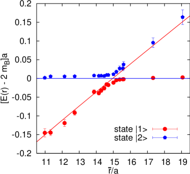
Figure 14: The same as Figure 13, for the string breaking region.

V.2 String breaking

In Figure 13 we plot the two energy levels, normalized with respect to $2m_{B}$, as a function of the $O(\alpha_{s})$ improved lattice distance $\overline{r}$, Eq. (40). Note that string breaking takes place at a distance $r_{c}\approx 15a\approx 1.25$ fm. The implications with respect to the $n_{f}=2+1$ QCD situation with realistic quark masses are discussed in Sec. VI below. The curve corresponds to the three-parameter fit,

$$E_{1}(r)=V_{0}+\sigma r-e/r,$$ (86)

with fit range $0.2\,\mbox{fm}\leq\overline{r}\leq 0.9$ fm. For the normalization we find, $V_{0}=2m_{B}-0.509(8)a^{-1}$ while string tension and Coulomb coefficient are respectively,

$$\sqrt{\sigma} = 0.1888(29)\,a^{-1},$$ (87)

$$e = 0.362(16).$$ (88)

The fit implies a Sommer parameter,

$$r_{0}^{2}\left.\frac{dE_{1}(r)}{dr}\right|_{r=r_{0}}=1.65,$$ (89)

of

$$r_{0}=6.009(53)a\approx 0.5\,\mbox{fm},$$ (90)

which we use to translate the lattice scale $a$ into physical units.

On the scale of Figure 13, the energy gap $\Delta E_{c}=\min_{r}[E_{2}(r)-E_{1}(r)]$ is barely visible. Therefore, we enlarge the string breaking region in Figure 14. We define the string breaking distance as the distance where the energy gap is minimal: $E_{2}(r_{c})-E_{1}(r_{c})=\Delta E_{c}$.

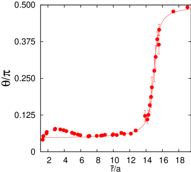
Figure 15: The mixing angle $\theta$, as a function of $\overline{r}$. The curve corresponds to the parametrization Eqs. (91)–(94).

Not only the two energy levels play a role in the mixing dynamics but also the mixing angle $\theta$ of Eqs. (83) and (84). In Figure 15 we depict $\theta$ as a function of $r$. For $r<r_{c}$, the overlap $Q_{1}$ will be larger than $B_{1}$ and hence $\theta<\pi/4$. For $r\rightarrow\infty$ the $\overline{Q}Q$ content of the ground state will vanish and $\theta\rightarrow\pi/2$. The Figure reveals that while this large $r$ limit is rapidly approached for $r>r_{c}$, the ground state at small $r$ contains a significant $B\overline{B}$ admixture: for instance, $\sin^{2}[\theta(8a)]\approx 0.03$. Furthermore, there is a “bump” at small $r$ in $\theta(r)$ as well as in $E_{2}(r)$, before $\theta$ is forced to approach zero at $r\rightarrow 0$, where $C_{QB}(t)=0$. This bump is likely to be related to light meson exchange, where in our study $m_{\pi}^{-1}\approx 4a$.

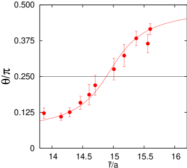
Figure 16: The same as Figure 15, for the string breaking region.

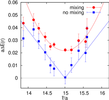
Figure 17: The energy gap $\Delta E=E_{2}-E_{1}$ with (circles) and without (squares) mixing.

The curve corresponds to a phenomenological three parameter fit to the $0.9\,\mbox{fm}\approx 11a\leq\overline{r}\leq 19a\approx 1.6\,\mbox{fm}$ data:

$$\theta(r)=\frac{c}{2}\left\{\arctan\left[d(r-r_{s})\right]-\frac{\pi}{2}\right\}+\frac{\pi}{2},$$ (91)

with parameter values,

$$r_{s} = 14.95(12)a,$$ (92)

$$d = 2.31(21)a^{-1},$$ (93)

$$c = 0.914(6).$$ (94)

The increase of $\theta$ with respect to $r$ for $r\approx r_{s}$ is given by, $d\theta(r)/dr|_{r=r_{s}}=cd/2=0.34(3)\pi\,a^{-1}$. Our distance-resolution clearly allows us to resolve the mixing dynamics at $r\approx r_{c}$. We enlarge this region in Figure 16.

Finally, in Figure 17, we investigate the difference $\Delta E(r)=E_{2}(r)-E_{1}(r)$ in the string breaking region. The circles represent the results from our mixing analysis while the squares are extracted from fits to the Wilson loops $C_{QQ}$ and the $I=1$ $B\overline{B}$ operator $C_{BB}^{\rm dis}$ alone. This resembles the situation in the quenched approximation where no string breaking or mixing occurs. We perform a quadratic fit in the region $14a\leq\overline{r}\leq 16a$,

$$\Delta E(r)=\Delta E_{c}+b^{3}(r-r_{c})^{2}.$$ (95)

The resulting parameter values are,

$$r_{c} = 15.00(8)\,a,$$ (96)

$$\Delta E_{c} = 0.0217(9)\,a^{-1},$$ (97)

$$b = 0.325(14)\,a^{-1}.$$ (98)

The position of the minimal energy gap $r_{c}=15.00(8)a$ is in perfect agreement with the value $r_{s}=14.95(12)a$ of Eq. (92), at which $\theta=\pi/4$. Translated into physical units we obtain a minimal energy gap, $\Delta E_{c}\approx 51(3)$ MeV, and a string breaking distance,

$$r_{c}=2.496(26)\,r_{0}\approx 1.248(13)\,\mbox{fm}.$$ (99)

The errors quoted are purely statistical and do not contain the 5 % uncertainty of $r_{0}\approx 0.5$ fm or the deviation of $n_{f}=2$ and $m\lesssim m_{s}$ from the real QCD situation.

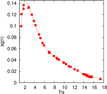
Figure 18: The transition rate $g$ between $|B\rangle$ and $|Q\rangle$ states, as a function of $\overline{r}$.

V.3 Transition rates

We assume that the elements of our mixing matrix only couple to the lowest two QCD eigenstates within the appropriate static-static sector. In this limit, for each $r$, we encounter a quantum mechanical two-state system. Our two test wave functions are not QCD eigenstates and, therefore, the off-diagonal matrix elements $C_{QB}(t)$ assume non-trivial values. The transition rate, governing string fission at $r>r_{c}$ and fusion at $r<r_{c}$, is given by,

$$g=\left.\frac{dC_{QB}(t)}{dt}\right|_{t=0}\frac{1}{\sqrt{C_{BB}(0)C_{QQ}(0)}}.$$ (100)

While in Euclidean time all Fock states eventually decay into the ground state $|1\rangle$, in Minkowski space-time, starting from such a non-eigenstate, results in oscillations between the $\overline{Q}Q$ and $B\overline{B}$ sectors.

Obviously, our states $|Q\rangle$ and $|B\rangle$ are somewhat polluted by $n\geq 3$ excitations as evidenced by $a_{Q}\neq 1$ and $a_{B}\neq 1$. So we have to “wait” for some initial relaxation time $t_{\min}$ to pass until this equation becomes applicable. We can easily extract $g$ from our five parameter fits, Eqs. (74) – (76), setting $C_{QQ}(0)=a_{Q}^{2}$ and $C_{BB}(0)=a_{B}^{2}$:

$$g(r)=\Delta E(r)\frac{\sin[2\theta(r)]}{2}.$$ (101)

This quantity is plotted in Figure 18 and the resulting values are displayed in the last column of Table 1. At the string breaking point, $\theta\approx\pi/4$ and hence $g(r_{c})\approx\Delta E_{c}/2\approx 25(2)$ MeV. This means that $g(r)$ has a maximal value of around 320 MeV, at a distance of about 0.2 fm. The curve is a polynomial and drawn to guide the eye. $g^{-1}$ can be interpreted as the characteristic Euclidean time scale, governing the decay of one state into the other. For instance, at $r=2a$ we find the (maximal) value $g^{-1}\approx 7.3a$ and indeed, in Figure 11, at $t/a>7$ the $C_{BB}$ effective masses (solid circles) agree with the $C_{QQ}$ level (open circles). We also find that the implicit indications of mixing effects are most pronounced at exactly the distance at which $g$ is largest.

For small $r$, $g$ decreases as it has to reach zero at $r=0$. At large $r$, $\theta$ approaches $\pi/2$ quite rapidly, resulting in small $g$ values too: for $r>r_{c}$ we find $g<\Delta E_{c}/2\approx 0.011\,a^{-1}$. This means that detecting the (dominantly $|B\rangle$) ground state of the system from Wilson loop signals alone necessitates distances $t=O(100\,a)$. Possibly, depending on the statistical accuracy, $t=50\,a$ might be sufficient to verify the decay of the Wilson loop signal towards the ground state energy. In view of this, it is no surprise that in Figure 12 we have been unable to verify such implicit string breaking at $r>r_{c}$ from $t\leq 9a$ data.

It is possible to calculate $g$ directly from the data, without any fits. This will be a valuable consistency check. For this purpose, the time derivative has to be eliminated from Eq. (100). It is straight forward to derive the approximate expression (for a similar result, see e.g. Michael Michael:2003vw ),

$$g(t)\approx Z\frac{C_{QB}(t)\sqrt{C_{QQ}(0)C_{BB}(0)}}{\sum_{j=1}^{t/a-1}C_{QQ}(ja)C_{BB}(t-ja)+\frac{1}{2}\left[C_{QQ}(0)C_{BB}(t)+C_{QQ}(t)C_{BB}(0)\right]},\quad Z=\frac{a\Delta E}{2\tanh(a\Delta E/2)}.$$ (102)

The $Z$ term originates from replacing a time integral by a discrete lattice sum. The required level difference $\Delta E$ can be approximated by an effective mass, however, for our proof-of-principle calculation we use the $\Delta E$ values of Table 1, extracted from our five parameter mixing fits. The largest such correction for the examples, displayed in Figure 19, amounts to a $3.7\,\%$ upward shift of the $r=2a$ data.

If the energy gap $\Delta E$ is large then, within the denominator, the propagation of the lighter state is strongly preferred over that of the heavier state and the transition between the two states will take place near the end points $j\approx 0$ or $j\approx t/a$. In this case, unless $E_{3}\gg E_{2}$, there will be higher state contaminations and no accurate result can be expected. If $\Delta E$ is large then $g=s_{\theta}c_{\theta}\Delta E$ can also be large. In the derivation of Eq. (102) implicit mixing effects are neglected and due to this, at large $t$, there will be corrections, $g=g(t)+O(gt)$. If $g$ is sufficiently small, then there is a chance of identifying a plateau in $g(t)$ from large enough (but not too large) $t$ values.

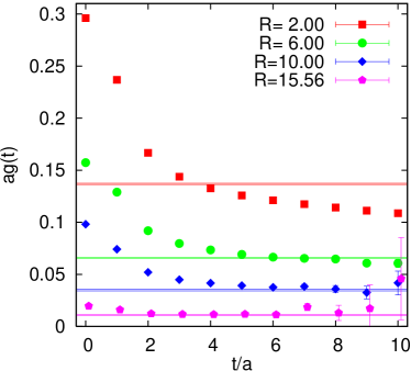
Figure 19: The modified Michael ratio Eq. (102) for different $r=Ra$ values, as a function of $t$. The horizontal error bands correspond to the fitted transition rates.

In Figure 19 we compare $g(t)$ approximants, obtained by use of the modified Michael ratio method Eq. (102), with our fitted $g$ values (horizontal error bands). We find good plateaus and perfect agreement with the fitted $g$ values, except at distances $r\leq 6a$ where implicit mixing is significant and the linear $t$ behaviour already sets in, before the excited state contributions have died out. In principle, one could attempt to subtract such linear terms.

The ratio method offers a nice check of consistency. Other than this, we see little advantage in calculating $g(t)$ over extracting $g$ from a global fit (in $t$) of the correlation matrix elements. In the case of very noisy data such fits may turn out impossible but in this case any $g(t)$ estimate will be unreliable anyhow. Note that within our fit ranges Eqs. (77)–(81), $g(t)$ does not show any sizeable excited state contaminations.

V.4 Short distance $B\overline{B}$ forces

We now focus on the short distance behaviour, both for $I=0$ and for $I=1$ $B\overline{B}$ systems, and display the respective two lowest lying energy levels in Figure 20. Note that the difference between the $I=1$ and the $I=0$ ground states is given by our (unrealistically heavy) $\pi$ mass, $m_{\pi}\approx 640$ MeV. The lowest state in the $I=0$ sector corresponds to the conventional $\overline{Q}Q$ potential. We already noted the bump in the excited state level, with a maximum of about 85(10) MeV, relative to $2m_{B}$, at a distance of 0.2 – 0.3 fm. Such a bump is not present within the $I=1$ sector, to which the exchange diagram $C_{BB}^{\rm con}$ does not contribute. We assume this energy barrier to be related to meson exchange. Note that at the distance of the maximum, $\Delta E(r)\approx 2m_{\pi}$. Unfortunately, in our study we restricted ourselves to one quark mass and hence we are unable to investigate the quark mass dependence of the height and of the position of this feature.

Within the $I=1$ situation, we also encounter two sectors, namely a $\overline{Q}Q\pi$ state (with $\overline{Q}Q$ in the $\Sigma_{u}^{-}$ representation that is mass-degenerate with $\Sigma_{g}^{+}$) and the $B\overline{B}$ state that we label as $|B_{a}\rangle$. After diagonalization of this mixing problem one should be able to identify a mixing angle $\phi$ and the two energy levels $E_{1}^{a}$ and $E_{2}^{a}$, in analogy to the $I=0$ system. Again, for $r=0$ the off-diagonal elements of the corresponding correlation matrix vanish and the two sectors decouple. The lower lying state will be a single $\pi$, with $\overline{Q}$ and $Q$ annihilating. In contrast, in this limit, $C_{BB}^{\rm dis}$ will couple to scalar states. In the colour singlet sector this will be a scalar $a_{0}$ meson as well as $\pi\pi$ scattering states. There will be excitations above these mesonic states, corresponding to two light quarks, bound to an adjoint static colour source, in analogy to pure gauge hybrid potentials where $\overline{Q}$ and $Q$ do not annihilate at $r=0$ (gluelumps Bali:2003jq ). Note that in the limit $r=0$, the $I=0$ correlation function $C_{BB}(t)$ will also couple to both, $B\overline{B}$ states with $q\bar{q}$ in a colour octet (which we shall call $q\bar{q}$ lumps) and to colour singlet $f_{0}/\pi\pi$ states. The latter sector is lighter.

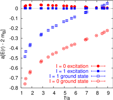
Figure 20: The first two energy levels within the $I=0$ and $I=1$ sectors, at short distances.

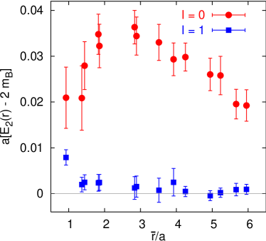
Figure 21: The $I=0$ and $I=1$ excited state energies, relative to $2m_{B}$, at short distances, $\overline{r}<r_{0}\approx 6a$.

As we only have the creation operator of the $|B_{a}\rangle$ state ${\mathcal{B}}_{a}$ at our disposal but do not separately investigate the $\overline{Q}Q\pi$ sector (and the mixing between the two sectors), we assume the lowest lying $I=1$ state (open squares) to consist of the ground state potential plus the mass of the $\pi$. There will be a (small) correction to this assumption, due to the interaction energy on a finite lattice. For the $r>2\sqrt{2}a$ data we are unable to detect this state within the $C_{BB}^{\rm dis}$ signal, see also Figure 9. For $\overline{r}<4a$ we apply two exponential fits with $t_{\min}=2a$. The overlap with the $\overline{Q}Q\pi$ ground state turns out to be tiny in these three parameter fits, with mixing angles ranging from $\sin^{2}(\phi)=0.0006(22)$ at $\overline{r}\approx 3.51a$ to $\sin^{2}(\phi)=0.0034(4)$ at $\overline{r}\approx 1.37a$. However, the fits are consistent with the ground state mass assumption, $E_{1}(r)+m_{\pi}$.

In Figure 21 we focus on the two $E_{2}$ levels at small $r$. As noted before, there is repulsion in the $I=0$ sector for distances $r>0.25$ fm, with a peak value of the energy barrier of about 85 MeV. However, at very short range, attraction sets in. This has to be so since in the $r\rightarrow 0$ limit the first excitation above the vacuum is a flavour singlet light quark state, with $\overline{Q}$ and $Q$ annihilating each other. Hence the form at asymptotically short distances will be governed by the perturbative colour singlet potential.

Contrary to Ref. Michael:1999nq , we also observe (weak) repulsion in the $I=1$ sector. This difference might be due to a bigger overlap of the ${\mathcal{B}}_{a}$ operator used in this previous study with the $\overline{Q}Q\pi$ ground state. However, with our operator and statistical accuracy we are able to clearly separate the (tiny) $\overline{Q}Q\pi$ pollution from $E_{2}$. From a four parameter two exponential fit to the $I=1$ operator $C_{BB}^{\rm dis}$ at $r=0$ we find, $aE_{1}=0.394(26)$, very similar to the corresponding $I=0$ value, $aE_{g}=0.32(17)$. This might indeed be a scalar $a_{0}$ meson. The coupling between our operator and this state is $a_{1}^{2}=0.010(2)$. The first excitation (with which our operator has 99 % overlap) that we are able to resolve is $E_{2}-2m_{B}=0.0079(16)a^{-1}$ (left most data point: $\overline{\mathbf{0}}\approx 0.92\,a$). We interpret this as the lowest lying lump of a $q\bar{q}$ state, bound to an adjoint static colour source. In this case the short distance interaction can be identified with the octet potential Bali:2003jq . As argued above, there should be further scattering states inbetween the $a_{0}$ level and the $q\bar{q}$ lump, however, our operator basis appears to have (almost) vanishing overlap with them.

VI Phenomenological implications

We discuss a possible extrapolation of our string breaking results to the $n_{f}=2+1$ case with realistic light quark masses. We also comment on the relevance of the results with respect to quarkonium spectroscopy.

VI.1 Extrapolation to real QCD

We expect the string breaking distance to decrease with the sea quark mass. From the experimental difference $m_{B_{s}}-m_{B}=90(3)$ MeV, we obtain $r_{c}\approx 2.16\,r_{0}\approx 1.08$ fm if we assume invariance of the shape of the $\overline{Q}Q$ potential under variation of the sea quark mass. This assumption however is rather arbitrary and we wish to refine this first very rough estimate.

A more controlled way is to extrapolate previous results of the static-light meson mass Struckmann:2000hm ; Bali:2003jv and of the $\overline{Q}Q$ energy Bali:2000vr quadratically in the $\pi$ mass. The latter extrapolation has already been performed in Ref. Bali:2000vr . For the static-light mass we obtain an upward shift, $\Delta m_{B}=0.21(10)\,r_{0}^{-1}$, when replacing our simulated quark mass by the physical light quark mass. This direction of change is possible since the self energy of the static propagator increases with decreasing sea quark mass Bali:2002wf . The potential at $r_{c}$ also moves upwards, unsurprisingly by an amount that is larger than $2\Delta m_{B}$. In combining the two extrapolations we obtain $r_{c}=(2.27\pm 0.20)\,r_{0}\approx(1.13\pm 0.10)$ fm for $n_{f}=2$ light sea quarks, in good agreement with the rough phenomenological estimate presented above.

The previous lattice results Bali:2000vr ; Struckmann:2000hm ; Bali:2003jv were obtained with a static action that differs from the present one where we employ fat temporal links (see Sec. III.2.2), however, this change will not affect the string breaking distance since, when introducing the fat link action, both energy levels are always shifted downwards by the same amount.

We discuss the effect of a third, heavier, sea quark flavour. In this case there will be two separate thresholds, one for the decay into what we call $B$ and $\overline{B}$ mesons and one into $B_{s}$ and $\overline{B}_{s}$. It is not a priori clear what effect the inclusion of such a third sea quark has on the $r_{c}$ position at which the decay into $B\overline{B}$ sets in. A comparison between the $n_{f}=0$ and the $n_{f}=2$ situations might give some indication. Interpolating the $n_{f}=0$ static-light masses of Refs. Allton:1994jz ; Ewing:1995ih to our quark mass, $m_{\pi}/m_{V}=0.704(5)$, we obtain the value $m_{B}=0.540(10)\,a^{-1}$ at $\beta=6.2$ where $r_{0}=7.30(4)\,a$. Together with the potential from Ref. Bali:1992ru , this corresponds to $r_{c}=2.53(8)\,r_{0}$, very consistent with our $n_{f}=2$ result, Eq. (99), $r_{c}=2.50(3)\,r_{0}$. So we would expect the value,

$$r_{c}=(2.27\pm 0.20)\,r_{0}\approx(1.13\pm 0.10)\,\mbox{fm},$$ (103)

to remain largely unaffected by the addition of the strange quark. Note that there are additional systematic errors of about $5~{}\%$ on the scale $r_{0}$ and that we have not attempted a continuum limit extrapolation. We expect large distance physics like the string breaking scenario to remain largely unaffected by charm quark dynamics which, however, might influence short distance interactions.

In Figure 22 we display our $n_{f}=2,m\lesssim m_{s}$ energy levels in physical units. The plotted parametrizations are,

$$E_{1}(r) = 2m_{B}+g_{1}(r)V(r)+c_{1},$$ (104)

$$E_{2}(r) = 2m_{B}+[1-g_{2}(r)]V(r)+c_{2},$$ (105)

where

$$g_{i}(r) = \frac{1}{2}-\frac{1}{\pi}\arctan\left[d_{i}(r-r_{c})\right],$$ (106)

$$V(r) = -e\left(\frac{1}{r}-\frac{1}{r_{c}}\right)+\sigma\left(r-r_{c}\right).$$ (107)

We use the $\arctan$ function in the definition of the smeared out step functions $g_{i}(r)$, rather than e.g. $\tanh$, to allow for a direct comparison with the dependence of the mixing angle $\theta$ on $r$, Eq. (91). Also note that the above parametrizations represent only effective descriptions of the data, within a certain window of distances $r<1.6$ fm. For instance, $E_{1}$ does not have the correct large distance limit $2m_{B}$. The parametrization of $E_{1}(r)$ is valid for $r>0.2$ fm, while that of $E_{2}(r)$ applies to $r>0.75$ fm. In this latter channel, we encounter a repulsive potential barrier at smaller distances, see Figures 13, 20 and 21.

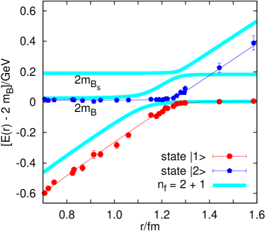
Figure 22: The energy levels in physical units for $n_{f}=2$ at a quark mass of slightly less than the strange quark mass (data points). The bands represent our $n_{f}=2+1$ speculation.

We use the same $e\approx 0.36$, $\sqrt{\sigma}\approx 447$ MeV as in Eqs. (87) – (88) and the $r_{c}\approx 1.25$ fm of Eq. (99). We obtain $c_{1}\approx-21$ MeV and $c_{2}\approx 31$ MeV. Note that $\Delta E_{c}=c_{2}-c_{1}\approx 51$ MeV. The parameters $d_{i}$ read, $d_{1}\approx 2.7\,\mbox{GeV}\approx(0.073\,\mbox{fm})^{-1}$, and $d_{2}\approx 4.0\,\mbox{GeV}\approx(0.049\,\mbox{fm})^{-1}$. Note that we parameterized the mixing angle in the string breaking region in a similar fashion, Eq. (91), with $d\approx 5.5$ GeV.

We speculate about the real QCD situation in Figure 22 (bands). Besides the above discussed reduction of the string breaking distance, we would expect the shape of the energy gap $\Delta E(r)$ to depend on the quark mass as well. A lighter mass will result in a larger gap $\Delta E_{c}$ and a broadened mixing region. We plot the corresponding curves with the arbitrary correction factors, $c_{i}\mapsto 1.5\,c_{i}$, $d_{i}\mapsto d_{i}/1.5$, also taking into account an increase of $e\approx 0.4$ and a reduction of $\sqrt{\sigma}\approx 440$ MeV Bali:1998pi . There will be a second level crossing around $2m_{B_{s}}$, which we also sketch in the Figure.

Another uncertainty is related to the short distance dynamics that we observe. We found an 85 MeV high potential barrier within $E_{2}(r)$, at a distance of about 0.2 fm. Most likely this is related to $\pi$ exchange Barnes:1999hs ; Tornqvist:2004qy . In this case the dimensions, both of the height of the barrier and of its position should be provided by the $\pi$ mass $m_{\pi}$. On one hand, reducing $m_{\pi}$ by a factor of four down to its physical value could easily move this region close to the string breaking distance. On the other hand, we would then expect the associated correction to the $E_{2}(r)$ level around $r_{c}$ to be smaller than 20 MeV, while $\Delta E_{c}>50$ MeV.

Finally, we remark that at smaller quark masses additional scattering states will occur between the $E_{1}(r)$ and the $E_{2}(r)$ energy levels, at short distances where $\Delta E(r)>2m_{\pi}$. It is clear that replacing our qualitative $n_{f}=2+1$ picture by a truly quantitative understanding would require simulations at additional light quark mass parameters.

VI.2 Relation to quarkonium physics

String breaking provides an intuitive example of a strong decay. In addition, static potentials can readily be related to quarkonium physics: this can be achieved by introducing a phenomenological Born-Oppenheimer approximation Eichten:1978tg or, more systematically, within the framework of potential NRQCD (pNRQCD) Brambilla:2004jw . As long as the quarkonium state in question is much lighter than the respective strong decay threshold into a pair of heavy-light mesons, the ground state energy level $E_{1}(r)$ should, to leading order in the relative $\overline{Q}Q$ velocity $v\ll 1$, accurately encapsulate the relevant physics. If this is not the case anymore, then additional terms have to be added to the pNRQCD Lagrangian, to incorporate the $\overline{Q}q\bar{q}Q$ sector and transitions between the two sectors: when it comes to strong decays like $\Upsilon(4S)\rightarrow B\overline{B}$, $E_{2}(r)$ and the transition rate/coupling $g(r)$ [or, equivalently, the mixing angle $\theta(r)$] are required to describe the system, in addition to $E_{1}(r)$.

For states that are stable against such decay, but which are in the vicinity of a threshold, mixing effects will result in mass shifts Eichten:1975ag ; Eichten:1978tg . This has been discussed in some detail for instance in Refs. Eichten:2004uh ; Barnes:2004fs ; Tornqvist:2004qy for the recently discovered $X(3872)$ charmonium state Choi:2003ue ; Brambilla:2004wf . In this context, our results could hint towards the nature of the underlying interaction Hamiltonian and of the $q\bar{q}$ pair creation mechanism that is at work.

We have demonstrated in Sec. V.3 that mixing is sufficiently weak to allow a basis of $\overline{Q}Q$ and $\overline{Q}q\bar{q}Q$ quark model Fock states to be a valid starting point in any such analysis Swanson:2005rc . However, not only in the string breaking region but also at short distances the ratio $g(r)/\Delta E(r)$ can be sizeable. We find $g(r)$ to be of an $O(100\,\mbox{MeV})$ magnitude which is typical for strong decay dynamics. $g(r)$ sets out from zero at the origin, increases to about 320 MeV around $r\approx 0.2$ fm and reduces to $\Delta E_{c}/2\approx 25$ MeV, in the string breaking region. The maximum value is due to meson exchange and its position coincides with, $\Delta E(r)\approx 2m_{\pi}\approx 4g(r)$. We would expect this medium range $g$ value to somewhat decrease with lighter quark masses and $g(r_{c})$ to increase.

In QCD with sea quarks there are not only $B\overline{B}$ excitations present but also $\overline{Q}Q$-gluon hybrid potentials. These however are energetically higher and, unless we are interested in hybrid quarkonia with spin-exotic quantum numbers, not a dominant correction Burch:2003zf to quark potential model predictions. Obviously, hybrid meson mixing and decay is interesting in itself McNeile:2002az , and, in this context, a detailed study of the breaking of hybrid strings would be interesting. Finally, at light sea quark masses hadronic transitions between quarkonia, mediated by $\pi$ radiation, become possible, the inclusion of which necessitates further modifications.

VII Summary

We were able to resolve the string breaking problem in $n_{f}=2$ QCD, at one value of the lattice spacing $a^{-1}\approx 2.37$ GeV and of the sea quark mass, $m\lesssim m_{s}$.

To achieve this result, the systematic improvement of our methods beyond the latest lattice technology was crucial. In particular, we used highly optimized smearing functions to enhance the overlap of our test wave functions with the physical states, we employed an improved static action and we realized many off-axis source separations. We used stochastic estimator techniques (SET) to calculate all-to-all propagators. The variance of SET was reduced by exactly calculating the contribution from the lowest lying eigenmodes of $\gamma_{5}M$, where $M$ denotes the Wilson Dirac matrix. Further variance reduction was achieved by the (new) hopping parameter acceleration (HPA) technique. These methods, most of which are neither specific to the string breaking problem nor to the static charge sector of lattice QCD, can readily be applied to a large spectrum of problems. In general we would expect the gain factor from HPA to decrease at lighter sea quark masses while the improved convergence of TEA should compensate for this.

We determined a mixing angle $\theta(r)$. Truncating the Fock basis after states containing four quark operators, the $\overline{Q}Q$ component of the physical ground state was given by $\sin\theta$ and the $B\overline{B}$ content by $\cos\theta$. We distinguished between the explicit and the implicit detection of mixing effects: a non-vanishing transition element between $\overline{Q}Q$ and $B\overline{B}$ states is an explicit signal of mixing. Additionally, at $r<r_{c}$ the ground state energy will dominate, even within the $B\overline{B}$ operator, at large Euclidean times (implicit mixing). We were able to verify this behaviour. At large $r>r_{c}$, the lowest lying state will have a mass slightly smaller than twice the static-light mass, $2m_{B}$, and dominantly couple to the $B\overline{B}$ operator. We were unable to detect this signal in the $\overline{Q}Q$ sector alone. Based on our mixing analysis, we expect such an implicit detection of string breaking to be almost hopeless, as high precision Wilson loop data at Euclidean times $t=O(5~{}\mbox{fm})$ would be necessary — and this at distances $r>1.2$ fm!

We defined two string breaking distances: $r_{c}=15.00(8)a\approx 1.248(13)$ fm denotes the distance at which the energy gap between the two levels $\Delta E(r)=E_{2}(r)-E_{1}(r)$ assumes its minimal value $\Delta E_{c}=0.022(1)a^{-1}\approx 51(3)$ MeV while $r_{s}=14.95(12)a\approx 1.244(16)$ fm denotes the distance of perfect mixing between the two states, in terms of the mixing angle $\theta(r_{s})=\pi/4$. The conversion into physical units has been made by setting $r_{0}=0.5$ fm. Note that $r_{c}-r_{s}=0.053(53)a$ is compatible with zero, within a standard deviation of less than $5\times 10^{-3}$ fm.

We would expect $\Delta E_{c}\approx 51(3)$ MeV to increase with lighter sea quark masses and hence this value should be regarded as a lower limit to the case with massless or very light sea quarks. In real QCD also the string breaking distance should decrease. We estimate $r_{c}=1.13(10)(10)$ fm for this case. The first error is statistical and from the chiral extrapolation of previous results, the second incorporates possible finite lattice spacing effects, the scale uncertainty in $r_{0}=0.5$ fm and effects due to the inclusion of a third active sea quark flavour. The qualitative situation is depicted in Figure 22.

We can define a transition rate $g(r)=\Delta E(r)\sin[2\theta(r)]/2$ between $\overline{Q}Q$ and $B\overline{B}$ states and note that $g(r_{s})=\Delta E(r_{s})/2$ and hence $g(r_{c})\approx\Delta E_{c}/2$. In the large $N_{c}$ limit this means that at leading order, $\Delta E_{c}\propto\sqrt{n_{f}/N_{c}}$, if we are interested in the screening of a fundamental string by a sea of $n_{f}$ massless flavours of fundamental particles, e.g. scalars or quarks. For the breaking of an adjoint string into two gluelumps the expectation reads, $\Delta E_{c}\propto 1/N_{c}$. In view of the precision of the $n_{f}=2$ QCD results presented here, it should be worthwhile to dedicate renewed effort onto string breaking studies of $SU(N_{c})$ gauge theories with and without Higgs fields, to confirm the expectations, and to explore the applicability of large $N_{c}$ arguments to strong hadronic decays.

We conclude that our study constitutes an important step towards the understanding of mixing effects and strong decays in quarkonium systems Eichten:2004uh ; Swanson:2005rc . Studying the energy between pairs of static-light mesons can also be viewed as a milestone with respect to a future calculation of $\Lambda_{Q}\Lambda_{Q}$ forces, which are related to nucleon-nucleon interactions Arndt:2003vx .