Abstract

This article is the written version of a talk delivered at the Workshop on Nonlinear Dynamics and Fundamental Interactions in Tashkent and starts with an introduction into quantum chaos and its relationship to classical chaos. The Bohigas-Giannoni-Schmit conjecture is formulated and evaluated within random-matrix theory. In accordance to the title, the presentation is twofold and begins with research results on quantum chromodynamics and the quark-gluon plasma. We conclude with recent research work on the spectroscopy of baryons. Within the framework of a relativistic constituent quark model we investigate the excitation spectra of the nucleon and the delta with regard to a possible chaotic behavior for the cases when a hyperfine interaction of either Goldstone-boson-exchange or one-gluon-exchange type is added to the confinement interaction. Agreement with predictions from the experimental hadron spectrum is established.

[Quantum chaos in QCD and hadrons] Quantum chaos in QCD and hadrons

1 Classical and Quantum Chaos

In order to understand in which manner classical chaos is reflected in quantum systems the question has been posed: Are there differences in the eigenvalue spectra of classically integrable and non-integrable systems? Billiards became a preferred playground to study both the classical and quantum case. With the arrival of computers with increasing power in the late seventies diagonalization of matrices with reasonable size became possible. The behavior of the distribution of the spacings between neighboring eigenvalues turned out to be a decisive signature. In 1979 McDonald and Kaufman performed a comparison between the spectra from a classically regular and a classically chaotic system [1]. As seen in Fig. 1 they observed a qualitatively different behavior between the nearest-neighbor spacing distribution of the circle and the stadium. In the first case the spacings are clearly concentrated around zero while they show repelling character in the second case. There were several authors contributing to this discussion and we mention the papers by Casati, Valz-Gris, and Guarneri [2], by Berry [3], by Robnik [4] and by Seligman, Verbaarschot, and Zirnbauer [5].

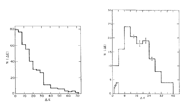
Figure 1: Nearest-neighbor spacing distributions of eigenvalues for a circle (left) and the Bunimovich stadium (right). Taken from Ref. [1].

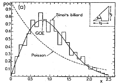
Figure 2: Nearest-neighbor spacing distributions of eigenvalues for the Sinai billiard with the Wigner surmise compared to the Poisson distribution. The histogram comprises about 1000 consecutive eigenvalues. Taken from Ref. [6].

Very accurate results were obtained for the classically chaotic Sinai billiard by Bohigas, Giannoni, and Schmit (see Fig. 2) which led them to the important conclusion [6]: Spectra of time-reversal invariant systems whose classical analogues are K systems show the same fluctuation properties as predicted by the Gaussian orthogonal ensemble (GOE) of random-matrix theory (RMT). K systems are most strongly mixing classical systems with a positive Kolmogorov entropy. The conjecture turned out valid also for less chaotic (ergodic) systems without time-reversal invariance leading to the Gaussian unitary ensemble (GUE).

2 Random Matrix Theory

In lack of analytical or numerical methods to obtain the spectra of complicated Hamiltonians, Wigner and Dyson analyzed ensembles of random matrices and were able to derive mathematical expressions. A Gaussian random matrix ensemble consists of square matrices with their matrix elements drawn from a Gaussian distribution

$$p(x)=\frac{1}{\sqrt{2\pi}\sigma}\;\exp\left(-\frac{x^{2}}{2\sigma^{2}}\right)\ .$$ (1)

One distinguishes between three different types depending on space-time symmetry classified by the Dyson parameter $\beta_{D}=1,2,4$ [7]. The Gaussian orthogonal ensemble (GOE, $\beta_{D}=1$) holds for time-reversal invariance and rotational symmetry of the Hamiltonian

$$H_{mn}=H_{nm}=H^{\ast}_{nm}\ .$$ (2)

When time-reversal invariance is violated and

$$H_{mn}=[H^{\dagger}]_{mn}\ ,$$ (3)

one obtains the Gaussian unitary ensemble (GUE, $\beta_{D}=2$). The Gaussian symplectic ensemble (GSE, $\beta_{D}=4$) is in correspondence with time-reversal invariance but broken rotational symmetry of the Hamiltonian

$$H^{(0)}_{nm}\mbox{1I}_{2}-i\sum\limits_{\gamma=1}^{3}H^{(\gamma)}_{nm}\sigma_{\gamma}\ ,$$ (4)

with $H^{(0)}$ real and symmetric and $H^{(\gamma)}$ real and antisymmetric.

The functional form of the distribution $P(s)$ of the neighbor spacings $s$ between consecutive eigenvalues for the Gaussian ensembles can be approximated by

$$P_{\beta_{D}}(s)=a_{\beta_{D}}\,s^{\beta_{D}}\exp\left(-b_{\beta_{D}}\,s^{2}\,\right)\ ,$$ (5)

which is known as the Wigner surmise and reads for example in the case $\beta_{D}=2$ (GUE)

$$P(s)=\frac{32}{\pi^{2}}\,s^{2}\exp\left(-\frac{4}{\pi}\,s^{2}\right)\ .$$ (6)

If the eigenvalues of a system are completely uncorrelated one ends up with a Poisson distribution for their neighbor spacings

$$P(s)=\exp{(-s)}\ .$$ (7)

An interpolating function between the Poisson and the Wigner distribution is given by the Brody distribution [8] reading for the GOE case

$$P(s,\omega)=\alpha\,(\omega+1)s^{\omega}\exp\left(-\alpha\,s^{\omega+1}\right)\ ,\quad\quad\alpha=\Gamma^{\omega+1}\,\left(\frac{\omega+2}{\omega+1}\right)\ ,$$ (8)

with $0\leq\omega\leq 1$.

Remarkably, the Wigner distribution could be observed in a number of systems by physical experiments and computer simulations evading the whole quantum world from atomic nuclei to the hydrogen atom in a magnetic field to the metal-insulator transition [7]. In this contribution we address the situation in QCD and in hadrons.

3 Quantum Chromodynamics

The Lagrangian ${\cal L}^{\mbox{\scriptsize QCD}}$ of quantum chromodynamics (QCD) consists of a gluonic part ${\cal L}_{\mbox{\scriptsize G}}^{\mbox{\scriptsize QCD}}$ and a part ${\cal L}_{\mbox{\scriptsize F}}^{\mbox{\scriptsize QCD}}$ from the quarks

$${\cal L}^{\mbox{\scriptsize QCD}} = {\cal L}_{\mbox{\scriptsize G}}^{\mbox{\scriptsize QCD}}+{\cal L}_{\mbox{\scriptsize F}}^{\mbox{\scriptsize QCD}}$$ (9)

$$= -\frac{1}{4}F_{\mu\nu}^{a}(x)F_{a}^{\mu\nu}(x)+\sum\limits_{f=1}^{N_{f}}\bar{\psi}_{f}(x)(iD\!\hbox to0.0pt{\hss/}-m_{f})\psi_{f}(x)\ ,$$

with the Dirac spinor $\psi_{f}$, the quark mass $m_{f}$, the number of flavors $N_{f}$, and the generalized field strength tensor

$$F_{a}^{\mu\nu}(x)=\partial^{\mu}A_{a}^{\nu}(x)-\partial^{\nu}A_{a}^{\mu}(x)-gf_{abc}A_{b}^{\mu}(x)A_{c}^{\nu}(x)\ ,$$ (10)

where the gauge field $A_{a}^{\mu}$ with the SU(3) indices $a,b,c=1,\dots,8$, the coupling constant $g$ and the structure constants $f_{abc}$ of SU(3) enter. The main object of study is the eigenvalue spectrum of the Dirac operator of QCD in 4 dimensions

$$\hbox{\large$/$}\kern-7.27847pt\hbox{$D$}=\hbox{\large$/$}\kern-5.65451pt\hbox{$\partial$}+ig\hbox{\large$/$}\kern-6.75pt\hbox{$A$}^{a}\frac{\lambda^{a}}{2}=\gamma_{\mu}\partial_{\mu}+ig\gamma_{\mu}A^{a}_{\mu}\frac{\lambda^{a}}{2}\ ,$$ (11)

with the $\lambda_{a}$ the generators of the SU(3) color-group (Gell-Mann matrices). Discretizing the Dirac operator on a lattice in Euclidean space-time and applying the Kogut-Susskind (staggered) prescription, leads to the matrix

$$(M_{\mbox{\scriptsize KS}})_{xx^{\prime}}^{aa^{\prime}}=\frac{1}{2a}\ \sum_{\mu}\left[\delta_{x+\hat{\mu},x^{\prime}}\ \Gamma_{x\mu}\ U_{x\mu}^{aa^{\prime}}-\delta_{x,x^{\prime}+\hat{\mu}}\ \Gamma_{x^{\prime}\mu}\ U^{\dagger\ aa^{\prime}}_{x^{\prime}\mu}\right]\ ,$$ (12)

where

$$U_{x\mu}=\exp\left(igA_{\mu}^{a}(x)\frac{\lambda^{a}}{2}\ \right)$$ (13)

are the gauge field variables on the lattice and $\Gamma_{x\mu}$ a representation of the $\gamma_{\mu}$-matrices.

In random matrix theory (RMT), one has to distinguish several universality classes which are determined by the symmetries of the system. For the case of the QCD Dirac operator, this classification was done in Ref. [9]. Depending on the number of colors and the representation of the quarks, the Dirac operator is described by one of the three chiral ensembles of RMT. As far as the fluctuation properties in the bulk of the spectrum are concerned, the predictions of the chiral ensembles are identical to those of the ordinary ensembles in Sect. 2 [10]. In Ref. [11], the Dirac matrix was studied for color-SU(2) using both Kogut-Susskind and Wilson fermions which correspond to the chiral symplectic (chSE) and orthogonal (chOE) ensemble, respectively. Here [12], we additionally study SU(3) with Kogut-Susskind fermions which corresponds to the chiral unitary ensemble (chUE). The RMT result for the nearest-neighbor spacing distribution can be expressed in terms of so-called prolate spheroidal functions, see Ref. [13]. A very good approximation to $P(s)$ is provided by the Wigner surmise for the unitary ensemble,

$$P_{\rm W}(s)=\frac{32}{\pi^{2}}s^{2}e^{-4s^{2}/\pi}\>.$$ (14)

We generated gauge field configurations using the standard Wilson plaquette action for SU(3) with and without dynamical fermions in the Kogut-Susskind prescription. We have worked on a $6^{3}\times 4$ lattice with various values of the inverse gauge coupling $\beta=6/g^{2}$ both in the confinement and deconfinement phase. We typically produced 10 independent equilibrium configurations for each $\beta$. Because of the spectral ergodicity property of RMT one can replace ensemble averages by spectral averages if one is only interested in bulk properties.

The Dirac operator, $\hbox{\large$/$}\kern-7.27847pt\hbox{$D$}=\hbox{\large$/$}\kern-5.65451pt\hbox{$\partial$}+ig\hbox{\large$/$}\kern-6.75pt\hbox{$A$}$, is anti-Hermitian so that the eigenvalues $\lambda_{n}$ of $i\hbox{\large$/$}\kern-7.27847pt\hbox{$D$}$ are real. Because of $\{\hbox{\large$/$}\kern-7.27847pt\hbox{$D$},\gamma_{5}\}=0$ the non-zero $\lambda_{n}$ occur in pairs of opposite sign. All spectra were checked against the analytical sum rules $\sum_{n}\lambda_{n}=0$ and $\sum_{\lambda_{n}>0}\lambda_{n}^{2}=3V$, where V is the lattice volume. To construct the nearest-neighbor spacing distribution from the eigenvalues, one first has to “unfold” the spectra [14].

	Confinement $\beta=5.2$			Deconfinement $\beta=5.4$
	$ma=0.05$			$ma=0.05$

Figure 3: Nearest-neighbor spacing distribution $P(s)$ for the Dirac operator on a $6^{3}\times 4$ lattice in full QCD (histograms) compared with the random matrix result (solid lines). There are no changes in $P(s)$ across the deconfinement phase transition.

Figure 4: Nearest-neighbor spacing distribution $P(s)$ for the free Dirac operator on a $53\times 47\times 43\times 41$ lattice compared with a Poisson distribution, $e^{-s}$.

Figure 4 compares $P(s)$ of full QCD with $N_{f}=3$ flavors and quark mass $ma=0.05$ to the RMT result. In the confinement as well as in the deconfinement phase we observe agreement with RMT up to very high $\beta$ (not shown). The observation that $P(s)$ is not influenced by the presence of dynamical quarks is expected from the results of Ref. [10], which apply to the case of massless quarks. Our results, and those of Ref. [11], indicate that massive dynamical quarks do not affect $P(s)$ either.

No signs for a transition to Poisson regularity are found. The deconfinement phase transition does not seem to coincide with a transition in the spacing distribution. For very large values of $\beta$ far into the deconfinement region, the eigenvalues start to approach the degenerate eigenvalues of the free theory, given by $\lambda^{2}=\sum_{\mu=1}^{4}\sin^{2}(2\pi n_{\mu}/L_{\mu})/a^{2}$, where $a$ is the lattice constant, $L_{\mu}$ is the number of lattice sites in the $\mu$-direction, and $n_{\mu}=0,\ldots,L_{\mu}-1$. In this case, the nearest-neighbor spacing distribution is neither Wigner nor Poisson. It is possible to lift the degeneracies of the free eigenvalues using an asymmetric lattice where $L_{x}$, $L_{y}$, etc. are relative primes and, for large lattices, the distribution is then Poisson, $P_{\rm P}(s)=e^{-s}$, see Fig. 4.

         

Figure 5: Nearest-neighbor spacing distribution $P(s)$ for U(1) gauge theory on an $8^{3}\times 6$ lattice in the confined phase (left) and in the Coulomb phase (right). The theoretical curves are the chUE result, Eq. (14), and the Poisson distribution, $P_{\rm P}(s)=\exp(-s)$.

We have also investigated the staggered Dirac spectrum of 4d U(1) gauge theory which corresponds to the chUE of RMT but had not been studied before in this context. At $\beta_{c}\approx 1.01$ U(1) gauge theory undergoes a phase transition between a confinement phase with mass gap and monopole excitations for $\beta<\beta_{c}$ and the Coulomb phase which exhibits a massless photon for $\beta>\beta_{c}$. As for SU(2) and SU(3) gauge groups, we expect the confined phase to be described by RMT, whereas free fermions are known to yield the Poisson distribution (see Fig. 4). The question arose whether the Coulomb phase would be described by RMT or by the Poisson distribution [15]. The nearest-neighbor spacing distributions for an $8^{3}\times 6$ lattice at $\beta=0.9$ (confined phase) and at $\beta=1.1$ (Coulomb phase), averaged over 20 independent configurations, are depicted in Fig. 5. Both are consistent with the chUE of RMT.

4 Hadrons

Taking the experimentally measured mass spectrum of hadrons up to 2.5 GeV from the Particle Data Group, Pascalutsa [16] could show that the hadron level-spacing distribution is remarkably well described by the Wigner surmise for $\beta=1$ (see Fig. 6). This indicates that the fluctuation properties of the hadron spectrum fall into the GOE universality class, and hence hadrons exhibit the quantum chaos phenomenon. One then should be able to describe the statistical properties of hadron spectra using RMT with random Hamiltonians from GOE that are characterized by good time-reversal and rotational symmetry.

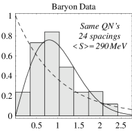
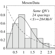
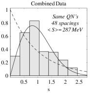
Figure 6: Histograms of the nearest-neighbor mass spacing distribution for hadron states with same quantum numbers. Curves represent the Poisson (dashed) and Wigner (solid) distributions. Taken from Ref. [16].

In order to test this experimental finding we are comparing with the eigenvalues of a Hamiltonian for a realistic quark model, namely the Goldstone-boson-exchange (GBE) constituent quark model [17]. It includes the kinetic energy in relativistic form

$$H_{0}=\sum\limits_{i=1}^{3}\sqrt{\vec{p}_{i}^{\;2}+m_{i}^{2}},$$ (15)

with $m_{i}$ the masses and $\vec{p}_{i}$ the 3-momenta of the constituent quarks. The interaction between two constituent quarks $i,j$

$$V(ij)=V_{\rm conf}(ij)+V_{\chi}(ij)$$ (16)

is given by a confinement potential in linear form

$$V_{\rm conf}(ij)=V_{0}+Cr_{ij}$$ (17)

and a hyperfine interaction consisting of only the spin-spin part of the pseudoscalar-meson-exchange potentials

$$\begin{array}[]{l}V_{\chi}(ij)=\left[\sum_{F=1}^{3}V_{\pi}(r_{ij})\lambda_{i}^{F}\lambda_{j}^{F}\right.+\sum_{F=4}^{7}V_{K}(r_{ij})\lambda_{i}^{F}\lambda_{j}^{F}\\[8.61108pt] \hskip 128.0374pt\left.+V_{\eta}(r_{ij})\lambda_{i}^{8}\lambda_{j}^{8}+\frac{2}{3}V_{\eta^{\prime}}(r_{ij})\right]\vec{\sigma}_{i}\cdot\vec{\sigma}_{j}.\end{array}$$ (18)

Here $r_{ij}$ is the distance between the quarks, $\vec{\sigma}_{i}$ are the Pauli spin matrices and $\lambda_{i}$ the Gell-Mann flavor matrices of the individual quarks. This kind of interaction is motivated by the spontaneous breaking of chiral symmetry. As a consequence constituent quarks and Goldstone bosons should be the appropriate effective degrees of freedom at low energies. Baryons are then assumed to be bound states of three confined constituent quarks with a hyperfine interaction relying on the exchange of the Goldstone bosons. Due to the specific flavor dependence in Eq. (18) a reasonable agreement between the spectra of the low lying light and strange baryon states calculated from the model and the experimental spectra could be achieved. In particular the ordering of the excited states with respect to their parities comes out correctly as is demonstrated in Fig. 7. It is interesting to notice that both the experiment and the numerical treatment have their problems to resolve the higher excited states.

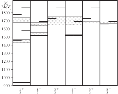
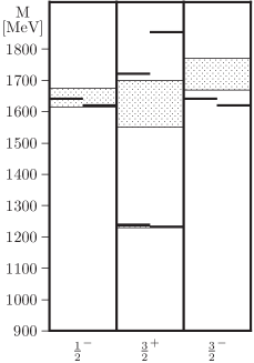
Figure 7: Low lying nucleon (left plot) and delta (right plot) states with total spin and parity $J^{\pi}$. The left and right bars are the theoretical energies predicted from the GBE and OGE models as described in the text, respectively. The shaded boxes represent the experimental energies with their uncertainties [18].

In order to investigate the influence of the hyperfine interaction we also analyze the nearest-neighbor spacings obtained with the confinement potential without the hyperfine interaction $V_{\chi}$ and with a model consisting of a different kind of hyperfine interaction which is based on one-gluon exchange (OGE). This was traditionally used in constituent quark models and has a flavor independent spin-spin potential. Therefore it has principal problems in reproducing the phenomenological ordering of the low lying excited nucleon states. Nevertheless, for comparison we consider here a simple version of such a model, i.e., a reparametrization of the Bhaduri, Cohler, and Nogami model consisting of a potential of the form

$$V(ij)=V_{0}+Cr_{ij}-\frac{2b}{3r_{ij}}+\frac{\alpha_{s}}{9m_{i}m_{j}}\Lambda^{2}\frac{e^{-\Lambda r_{ij}}}{r_{ij}}\vec{\sigma}_{i}\vec{\sigma}_{j},$$ (19)

and also a relativistic kinetic energy term in its Hamiltonian [19]. The spectra of the low lying nucleon and delta states calculated with this model are inserted in Fig. 7.

Figure 8: Histograms of the nearest-neighbor spacing distribution for the nucleon (left plots) and the delta (right plots). The data is for Goldstone-boson exchange and for one-gluon exchange compared to a pure linear confinement potential of the same strength. Curves represent the Poisson and the GOE-Wigner distributions.

In Fig. 8 we present our theoretical results of the nearest-neighbor spacing distribution for the nucleon and the delta. Both the hyperfine interaction of either Goldstone-boson exchange and one-gluon exchange type yield spacing distributions corresponding to the GOE. One observes a preference for the GOE from the linear rise at the origin while the other ensembles are quadratic or quartic (cf. Eq. 5). It turns out that the linear confinement potential alone without reproducing the spectra yields eigenvalues with reduced correlations between their neighbors and thus leading towards a Poisson distribution, as seen clearly from the nucleon in Fig. 8.

5 Conclusion

We have outlined the universal applicability of random-matrix theory and have presented own studies of quantum chromodynamics and hadrons. Concerning QCD, we were able to demonstrate that the nearest-neighbor spacing distribution $P(s)$ of the eigenvalues of the Dirac operator agrees perfectly with the RMT prediction both in the confinement and quark-gluon plasma-phase. This means that QCD is governed by quantum chaos in both phases. We could show that the eigenvalues of the free Dirac theory yield a Poisson distribution related to regular behavior. Our investigations tell us that the critical point of the spontaneous breaking of chiral symmetry does not coincide with a chaos-to-order transition. Concerning quarks building hadrons, we employed a relativistic quark potential model allowing for meson exchange or one-gluon exchange. Computing the spectrum of the nucleon and delta baryon indicates a spacing distribution $P(s)$ favoring the GOE of RMT. A linear confinement potential alone without reproducing the level ordering is not enough to obtain the correct fluctuations between the eigenvalues. Our results are in agreement with an analysis of the experimental mass spectrum of hadrons from the Particle Data Tables. Invoking the Bohigas-Giannoni-Schmit conjecture, we conclude that not only the quarks but also the hadrons show evidence of quantum chaos.

1

References

- [1] S.W. McDonald and A.N. Kaufman, Phys. Rev. Lett. 42 (1979) 1189.
- [2] G. Casati, F. Valz-Gris, and I. Guarneri, Lett. Nuovo Cimento 28 (1980) 279.
- [3] M.V. Berry, Ann. Phys. (NY) 131 (1981) 163.
- [4] M. Robnik, J. Phys. A 17 (1984) 1049.
- [5] T.H. Seligman, J.J.M. Verbaarschot, and M.R. Zirnbauer, Phys. Rev. Lett. 53 (1984) 215; T.H. Seligman, J.J.M. Verbaarschot, and M.R. Zirnbauer, J. Phys. A 18 (1985) 2751.
- [6] O. Bohigas, M.-J. Giannoni, and C. Schmit, Phys. Rev. Lett. 52 (1984) 1.
- [7] T. Guhr, A. Müller-Groeling, and H.A. Weidenmüller, Phys. Rep. 299 (1998) 189.
- [8] T.A. Brody, Lett. Nuovo Cimento 7 (1973) 482.
- [9] J.J.M. Verbaarschot, Phys. Rev. Lett. 72 (1994) 2531.
- [10] D. Fox and P.B. Kahn, Phys. Rev. 134 (1964) B1151; T. Nagao and M. Wadati, J. Phys. Soc. Jpn. 60 (1991) 3298; 61 (1992) 78; 61 (1992) 1910.
- [11] M.A. Halasz and J.J.M. Verbaarschot, Phys. Rev. Lett. 74 (1995) 3920; M.A. Halasz, T. Kalkreuter, and J.J.M. Verbaarschot, Nucl. Phys. B (Proc. Suppl.) 53 (1997) 266.
- [12] R. Pullirsch, K. Rabitsch, T. Wettig, and H. Markum, Phys. Lett. B 427 (1998) 119.
- [13] M.L. Mehta, Random Matrices, 2nd Ed. (Academic Press, San Diego, 1991).
- [14] O. Bohigas and M.-J. Giannoni, Springer Lect. Notes Phys. 209 (1984) 1.
- [15] B.A. Berg, H. Markum, and R. Pullirsch, Phys. Rev. D 59 (1999) 097504.
- [16] V. Pascalutsa, Eur. Phys. J. A 16 (2003) 149.
- [17] L.Y. Glozman, W. Plessas, K. Varga, and R.F. Wagenbrunn, Phys. Rev. D 58 (1998) 094030.
- [18] S. Eidelman et al. [Particle Data Group Collaboration], Phys. Lett. B 592 (2004) 1.
- [19] L. Theußl, R.F. Wagenbrunn, B. Desplanques, and W. Plessas, Eur. Phys. J. A 12 (2001) 91.